Neutrino Decay and Atmospheric Neutrinos

Abstract

We reconsider neutrino decay as an explanation for atmospheric neutrino observations. We show that if the mass-difference relevant to the two mixed states $\nu_{\mu}$ and $\nu_{\tau}$ is very small $(<10^{-4}\rm\,eV^{2})$, then a very good fit to the observations can be obtained with decay of a component of $\nu_{\mu}$ to a sterile neutrino and a Majoron. We discuss how the K2K and MINOS long-baseline experiments can distinguish the decay and oscillation scenarios.

Recently a neutrino decay explanation for the atmospheric neutrino observations of Super-Kamiokande was proposed[1]. To recapitulate briefly, in presence of a decaying neutrino state, the survival probability of $\nu_{\mu}$ is given by

$$P(\nu_{\mu}\to\nu_{\mu})=\sin^{4}\theta+\cos^{4}\theta e^{-\alpha L/E}+2\sin^{2}\theta\cos^{2}\theta e^{-\alpha L/2E}\cos\left(\frac{\delta m_{23}^{2}L}{2E}\right)$$ (1)

where we have considered only two state mixing for simplicity: $\delta m_{23}^{2}=m^{2}_{2}-m^{2}_{3},\ \alpha=m_{2}/\tau_{2}$ and $\nu_{\mu}=\cos\theta\nu_{2}+\sin\theta\nu_{3}$. If the decay of $\nu_{2}$ is $\nu_{2}\rightarrow\bar{\nu}_{3}+J$, where J is a massless scalar, then the $\delta m^{2}$ in the decay is the same as in Eq. (1) and it can be shown that this $\delta m^{2}$ has to be larger than 0.73 eV² to satisfy constraints from $K\to\mu+\rm neutrals$ decay[2]. Then the oscillating term in Eq. (1) averages to zero and $P(\nu_{\mu}\to\nu_{\mu})$ simplifies to

$$P(\nu_{\mu}\to\nu_{\mu})=\sin^{4}\theta\ +\cos^{4}\theta e^{-\alpha L/E}$$ (2)

This decay scenario was analyzed in Ref. [1] and fit to the $L/E_{\nu}$ dependence and the asymmetry of the contained events in Super-Kamiokande[3]. A satisfactory fit with $\cos^{2}\theta\sim 0.87$ and $\alpha\sim 1~{}{\rm GeV}/D_{E}$ (where $D_{E}$ is the diameter of the earth) was found. However, it has since been shown that the fit to the higher energy events in Super-K (especially the upcoming muons) is quite poor[4], [5].

Another possibility, mentioned in Ref. [1], is that the decay of $\nu_{2}$ is into a state with which it does not mix. For example, the three weak coupling states $\nu_{\mu},\nu_{\tau},\nu_{s}$ (where $\nu_{s}$ is a sterile neutrino) may be related to the mass eigenstates $\nu_{2},\nu_{3},\nu_{4}$ by the approximate mixing

$$\left(\begin{array}[]{c}\nu_{\mu}\\ \nu_{\tau}\\ \nu_{s}\end{array}\right)=\left(\begin{array}[]{ccc}\cos\theta&\sin\theta&0\\ -\sin\theta&\cos\theta&0\\ 0&0&1\end{array}\right)\left(\begin{array}[]{c}\nu_{2}\\ \nu_{3}\\ \nu_{4}\end{array}\right)$$ (3)

and the decay is $\nu_{2}\to\bar{\nu}_{4}+J$. The electron neutrino, which we identify with $\nu_{1}$, cannot mix very much with the other three because of the more stringent bounds on its couplings[2], and thus our preferred solution for solar neutrinos would be small angle matter oscillations.

Then the $\delta m_{23}^{2}$ in Eq. (1) is not related to the $\delta m_{24}^{2}$ in the decay, and can be very small, say $<10^{-4}\rm\,eV^{2}$ (to ensure that oscillations play no role in the atmospheric neutrinos). In that case, the oscillating term is 1 and $P(\nu_{\mu}\to\nu_{\mu})$ becomes

$$P(\nu_{\mu}\to\nu_{\mu})=(\sin^{2}\theta+\cos^{2}\theta e^{-\alpha L/2E})^{2}$$ (4)

This is identical to Eq. (13) in Ref. [1]. Here we consider this decay model and compare it to observations.

In order to compare the predictions of this model with the standard $\nu_{\mu}\leftrightarrow\nu_{\tau}$ oscillation model, we have calculated with Monte Carlo methods the event rates for contained, semi-contained and upward-going (passing and stopping) muons in the Super-K detector, in the absence of ‘new physics’, and modifying the muon neutrino flux according to the decay or oscillation probabilities discussed above. We have then compared our predictions with the SuperK data [3], calculating a $\chi^{2}$ to quantify the agreement (or disagreement) between data and calculations. In performing our fit (see Ref. [4] for details) we do not take into account any systematic uncertainty, but we allow the absolute flux normalization to vary as a free parameter $\beta$.

The ‘no new physics model’ gives a very poor fit to the data with $\chi^{2}=281$ for 34 d.o.f. (35 bins and one free parameter, $\beta$). For the standard $\nu_{\mu}\leftrightarrow\nu_{\tau}$ oscillation scenario the best fit has $\chi^{2}=33.3$ (32 d.o.f.) and the values of the relevant parameters are $\Delta m^{2}=3.2\times 10^{-3}$ eV², $\sin^{2}2\theta=1$ and $\beta=1.15$. This result is in good agreement with the detailed fit performed by the SuperK collaboration [3] giving us confidence that our simplified treatment of detector acceptances and systematic uncertainties is reasonable. The decay model of Equations (3) and (4) above gives an equally good fit with a minimum $\chi^{2}=33.7$ (32 d.o.f.) for the choice of parameters

$$\tau_{\nu}/m_{\nu}=63\rm~{}km/GeV,\ \cos^{2}\theta=0.30$$ (5)

and normalization $\beta=1.17$.

In Fig. 1 we compare the best fits of the two models considered (oscillations and decay) with the SuperK data. In the figure we show (as data points with statistical error bars) the ratios between the SuperK data and the Monte Carlo predictions calculated in the absence of oscillations or other form of ‘new physics’ beyond the standard model. In the six panels we show separately the data on $e$-like and $\mu$-like events in the sub-GeV and multi-GeV samples, and on stopping and passing upward-going muon events. The solid (dashed) histograms correspond to the best fits for the decay model ($\nu_{\mu}\leftrightarrow\nu_{\tau}$ oscillations). One can see that the best fits of the two models are of comparable quality. The reason for the similarity of the results obtained in the two models can be understood by looking at Fig. 2, where we show the survival probability $P(\nu_{\mu}\to\nu_{\mu})$ of muon neutrinos as a function of $L/E_{\nu}$ for the two models using the best fit parameters. In the case of the neutrino decay model (thick curve) the probability $P(\nu_{\mu}\to\nu_{\mu})$ monotonically decreases from unity to an asymptotic value $\sin^{4}\theta\simeq 0.49$. In the case of oscillations the probability has a sinusoidal behaviour in $L/E_{\nu}$. The two functional forms seem very different; however, taking into account the resolution in $L/E_{\nu}$, the two forms are hardly distinguishable. In fact, in the large $L/E_{\nu}$ region, the oscillations are averaged out and the survival probability there can be well approximated with 0.5 (for maximal mixing). In the region of small $L/E_{\nu}$ both probabilities approach unity. In the region $L/E_{\nu}$ around 400 km/GeV, where the probability for the neutrino oscillation model has the first minimum, the two curves are most easily distinguishable, at least in principle.

Decay Model

There are two decay possibilities that can be considered: (a) $\nu_{2}$ decays to $\bar{\nu}_{4}$ which is dominantly $\nu_{s}$ with $\nu_{2}$ and $\nu_{3}$ mixtures of $\nu_{\mu}$ and $\nu_{\tau}$, as in Eq. (3), and (b) $\nu_{2}$ decays into $\bar{\nu}_{4}$ which is dominantly $\bar{\nu}_{\tau}$ and $\nu_{2}$ and $\nu_{3}$ are mixtures of $\nu_{\mu}$ and $\nu_{s}$. In both cases the decay interaction has to be of the form

$${\cal{L}}_{int}=g_{24}\ \overline{\nu_{4_{L}}^{c}}\ \nu_{2_{L}}J+h.c.$$ (6)

where $J$ is a Majoron field that is dominantly iso-singlet (this avoids any conflict with the invisible width of the $Z$). Viable models for both the above cases can be constructed [6, 7]. However, case (b) needs additional iso-triplet light scalars which cause potential problems with Big Bang Nucleosynthesis (BBN), and there is some preliminary evidence from SuperK against $\nu_{\mu}$–$\nu_{s}$ mixing [8]. Hence we only consider case (a), i.e. $\nu_{2}\to\bar{\nu}_{4}+J$ with $\nu_{4}\approx\nu_{s}$, as implicit in Eq. (3). With this interaction, the $\nu_{2}$ rest-lifetime is given by

$$\tau_{2}=\frac{16\pi}{g^{2}}\cdot\ \frac{m_{2}}{\delta m^{2}(1+x)^{2}},$$ (7)

where $\delta m^{2}=m^{2}_{2}-m^{2}_{4}$ and $x=m_{4}/m_{2}\ (0<x<1)$. From the value of $\alpha^{-1}=\tau_{2}/m_{2}=63$ km/GeV found in the fit and for $x=0$, we have

$$g^{2}\delta m^{2}\simeq 0.16\rm\,eV^{2}$$ (8)

Combining this with the bound on $g^{2}$ from $K\rightarrow\mu$ decays of $g^{2}<2.4\times 10^{-4}$ [2] we have

$$\delta m^{2}>650\rm\ eV^{2}\,.$$ (9)

Even with a generous interpretation of the uncertainties in the fit, this $\delta m^{2}$ implies a minimum mass difference in the range of about 25 eV. Then $\nu_{2}$ and $\nu_{3}$ are nearly degenerate with masses $\gtrsim{\cal O}$(25 eV) and $\nu_{4}$ is relatively light. We assume that a similar coupling of $\nu_{3}$ to $\nu_{4}$ and J is somewhat weaker leading to a significantly longer lifetime for $\nu_{3}$, and the instability of $\nu_{3}$ is irrelevant for the analysis of the atmospheric neutrino data.

For the atmospheric neutrinos in SuperK, two kinds of tests have been proposed to distinguish between $\nu_{\mu}$–$\nu_{\tau}$ oscillations and $\nu_{\mu}$–$\nu_{s}$ oscillations. One is based on the fact that matter effects are present for $\nu_{\mu}$–$\nu_{s}$ oscillations[9] but are nearly absent for $\nu_{\mu}$–$\nu_{\tau}$ oscillations[10] leading to differences in the zenith angle distributions due to matter effects on upgoing neutrinos [11]. The other is the fact that the neutral current rate will be affected in $\nu_{\mu}$–$\nu_{s}$ oscillations but not for $\nu_{\mu}$–$\nu_{\tau}$ oscillations as can be measured in events with single $\pi^{0}$’s [12]. In these tests our decay scenario will behave as a hybrid in that there is no matter effect but there is some effect in neutral current rates.

Long-Baseline Experiments

The survival probability of $\nu_{\mu}$ as a function of $L/E$ is given in Eq. (1). The conversion probability into $\nu_{\tau}$ is given by

$$P(\nu_{\mu}\to\nu_{\tau})=\sin^{2}\theta\cos^{2}\theta(1-e^{-\alpha L/2E})^{2}\,.$$ (10)

This result differs from $1-P(\nu_{\mu}\to\nu_{\mu})$ and hence is different from $\nu_{\mu}$–$\nu_{\tau}$ oscillations. Furthermore, $P(\nu_{\mu}\to\nu_{\mu})+P(\nu_{\mu}\to\nu_{\tau})$ is not 1 but is given by

$$P(\nu_{\mu}\to\nu_{\mu})+P(\nu_{\mu}\to\nu_{\tau})=1-\cos^{2}\theta(1-e^{-\alpha L/E})$$ (11)

and determines the amount by which the predicted neutral-current rates are affected compared to the no oscillations (or the $\nu_{\mu}$–$\nu_{\tau}$ oscillations) case. In Fig. 3 we give the results for $P(\nu_{\mu}\to\nu_{\mu})$, $P(\nu_{\mu}\to\nu_{\tau})$ and $P(\nu_{\mu}\to\nu_{\mu})+P(\nu_{\mu}\to\nu_{\tau})$ for the decay model and compare them to the $\nu_{\mu}$–$\nu_{\tau}$ oscillations, for both the K2K[13] and MINOS[14] (or the corresponding European project[15]) long-baseline experiments, with the oscillation and decay parameters as determined in the fits above.

The K2K experiment, already underway, has a low energy beam $E_{\nu}\approx 1\mbox{--}2$ GeV and a baseline $L=250$ km. The MINOS experiment will have 3 different beams, with average energies $E_{\nu}=3,$ 6 and 12 GeV and a baseline $L=732$ km. The approximate $L/E_{\nu}$ ranges are thus 125–250 km/GeV for K2K and 50–250 km/GeV for MINOS. The comparisons in Figure 3 show that the energy dependence of $\nu_{\mu}$ survival probability and the neutral current rate can both distinguish between the decay and the oscillation models. MINOS and the European project may also have $\tau$ detection capabilities that would allow additional tests.

Big Bang Nucleosynthesis

The decay of $\nu_{2}$ is sufficiently fast that all the neutrinos ($\nu_{e},\nu_{\mu},\nu_{\tau},\nu_{s}$) and the Majoron may be expected to equilibrate in the early universe before the primordial neutrinos decouple. When they achieve thermal equilibrium each Majorana neutrino contributes $N_{\nu}=1$ and the Majoron contributes $N_{\nu}=4/7$ [16], giving and effective number of light neutrinos $N_{\nu}=4{4\over 7}$ at the time of Big Bang Nucleosynthesis. From the observed primordial abundances of ⁴He and ⁶Li, upper limits on $N_{\nu}$ are inferred, but these depend on which data are used[17, 18, 19]. Conservatively, the upper limit to $N_{\nu}$ could extend up to 5.3 (or even to 6 if ⁷Li is depleted in halo stars[17]).

Cosmic Neutrino Fluxes

Since we expect both $\nu_{2}$ and $\nu_{3}$ to decay, neutrino beams from distant sources (such as Supernovae, active galactic nuclei and gamma-ray bursters) should contain only $\nu_{e}$ and $\bar{\nu}_{e}$ but no $\nu_{\mu}$, $\bar{\nu}_{\mu}$, $\nu_{\tau}$ and $\bar{\nu}_{\tau}$. This is a very strong prediction of our decay scenario.

Reactor and Accelerator Limits

The $\nu_{e}$ is essentially decoupled from the decay state $\nu_{2}$ so the null observations from the CHOOZ reactor are satisfied[20]. The mixings of $\nu_{\mu}$ and $\nu_{\tau}$ with $\nu_{s}$ and $\nu_{e}$ are very small, so there is no conflict with stringent accelerator limits on flavor oscillations with large $\delta m^{2}$ [21].

Conclusions

In summary, we have shown that neutrino decay remains a viable alternative to neutrino oscillations as an explanation of the atmospheric neutrino anomaly. The model consists of two nearly degenerate mass eigenstates $\nu_{2}$, $\nu_{3}$ with mass separation $\gtrsim{\cal O}(25$ eV) from another nearly degenerate pair $\nu_{1}$, $\nu_{4}$. The $\nu_{\mu}$ and $\nu_{\tau}$ flavors are approximately composed of $\nu_{2}$ and $\nu_{3}$, with a mixing angle $\theta_{23}\simeq 57^{\circ}$. The state $\nu_{2}$ is unstable, decaying to $\bar{\nu}_{4}$ and a Majoron with a lifetime $\tau_{2}\sim 10^{-12}$ sec. The electron neutrino $\nu_{e}$ and a sterile neutrino $\nu_{s}$ have negligible mixing with $\nu_{\mu},\nu_{\tau}$ and are approximate mass eigenstates ($\nu_{e}\approx\nu_{1},\nu_{s}\approx\nu_{4})$, with a small mixing angle $\theta_{14}$ and a $\delta m_{41}^{2}\approx 10^{-5}\rm\,eV^{2}$ to explain the solar neutrino anomaly. The states $\nu_{3}$ and $\nu_{4}$ are also unstable, but with $\nu_{3}$ lifetime somewhat longer and $\nu_{4}$ lifetime much longer than the $\nu_{2}$ lifetime. This decay scenario is difficult to distinguish from oscillations because of the smearing in both L and $E_{\nu}$ in atmospheric neutrino events. However, long-baseline experiments, where $L$ is fixed, should be able to establish whether the dependence of $L/E_{\nu}$ is exponential or sinusoidal. In our scenario only $\nu_{1}$ is stable. Thus, neutrinos of supernovae or of extra galactic origin would be almost entirely $\nu_{e}$. The contribution of the electron neutrinos and the Majorons to the cosmological energy density $\Omega$ is negligible and not relevant for large scale structure formation.

Acknowledgements

We would like to thank A. Joshipura for useful discussions. This work is supported in part by the U.S. Department of Energy.

FIG. 1.: Comparison of decay model (solid histograms) and $\nu_{\mu}$–$\nu_{\tau}$ oscillation model (dashed histograms) with SuperK data from Ref. [3].

FIG. 2.: Survival probabiliity for $\nu_{\mu}$ versus $\log_{10}(L/E)$ for the decay model (heavy solid curve) and $\nu_{\mu}$ oscillation model (thin curve).

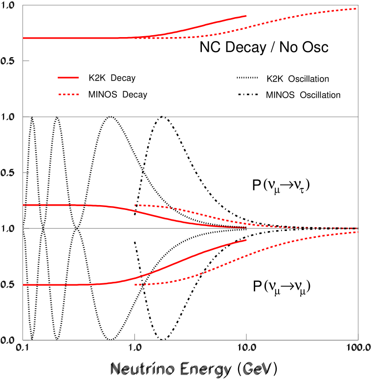
FIG. 3.: Long-baseline expectations for the K2K and MINOS long-baseline experiments from the decay model and the $\nu_{\mu}$–$\nu_{\tau}$ oscillation model. The upper panel gives the neutral current predictions compared to no oscillations (or $\nu_{\mu}$–$\nu_{\tau}$ oscillations).

REFERENCES

- [1] V. Barger, J.G. Learned, S. Pakvasa and T.J. Weiler, Phys. Rev. Lett 82, 2640 (1999).
- [2] V. Barger, W-Y. Keung and S. Pakvasa, Phys. Rev. D25, 907 (1982).
- [3] Y. Fukuda et al. (the Super-Kamiokande Collaboration), Phys. Rev. Lett. 81, 1562 (1998); Y. Fukuda et al. (the Super-Kamiokande Collaboration), Phys. Rev. Lett. 82, 2644 (1998); T. Kajita, hep-ex/9810001. The use of more recent data (K. Scholberg, hep-ph/9905016) does not change the conclusions.
- [4] P. Lipari and M. Lusignoli, Phys. Rev. D60, 013003 (1999).
- [5] G. Fogli, E. Lisi and A. Marrone, Phys. Rev. D59, 117303 (1999); S. Choubey and S. Goswami, hep-ph/9904257.
- [6] J. Valle, Phys. Lett. B131, 87 (1983); G. Gelmini and J. Valle, Phys. Lett. B142, 181 (1983); A. Joshipura and S. Rindani, Phys. Rev. D46, 300 (1992); K. Choi and A. Santamaria, Phys. Lett. B267, 504 (1991); A. Acker, A. Joshipura and S. Pakvasa, Phys. Lett. B285, 371 (1992).
- [7] A. Joshipura (private communication).
- [8] T. Kajita, Super-Kamiokande results presented at the “Beyond the Desert” Workshop, Castle Ringberg, Tegernsee, Germany, June 6–12, 1999 (to be published in the proceedings).
- [9] V. Barger, N. Deshpande, P. Pal, R.J.N. Phillips and K. Whisnant, Phys. Rev. D43, 1759 (1991); E. Akhmedov, P. Lipari and M. Lusignoli, Phys. Lett. B300, 128 (1993).
- [10] J. Pantaleone, Phys. Rev. D49, 2152 (1994).
- [11] Q. Liu and A. Smirnov, Nucl. Phys. B524, 505 (1998); P. Lipari and M. Lusignoli, Phys. Rev. D58, 073005 (1998).
- [12] F. Vissani and A. Smirnov, Phys. Lett B432, 376 (1998); J. Learned, S. Pakvasa, and J. Stone, Phys. Lett. B435, 131 (1998).
- [13] KEK-PS E362, INS-924 report (1992).
- [14] MINOS Collaboration, NuMI-L-375 report (1998).
- [15] NGS report, CERN 98-02, INFN/AE-98/05 (1998).
- [16] R. Kolb and M. S. Turner, The Early Universe, Addison - Wesley (1990).
- [17] K. Olive and D. Thomas, hep-ph/9811444.
- [18] E. Lisi, S. Sarkar, F. Villante, Phys. Rev. D59, 123520 (1999).
- [19] S. Burles, K. Nollett, J. Truran and M. S. Turner, Phys. Rev. Lett. 82, 4176 (1999).
- [20] M. Apollonio et al. (the CHOOZ Collaboration), Phys. Lett. B420, 320 (1998).
- [21] For a review of accelerator limits, see K. Zuber, Phys. Rep. 305, 295 (1998).