Generalized Dipole Polarizabilities of the Pion

Abstract

We discuss the virtual Compton scattering amplitude $\gamma^{\ast}+\pi\to\gamma+\pi$ which enters the reaction $\pi^{-}+e^{-}\to\pi^{-}+e^{-}+\gamma$. The low-energy scattering amplitude is divided into a model-independent part, involving only the electromagnetic form factor, and a residual part which contains structure information related specifically to (virtual) Compton scattering. In the limit of vanishing final-photon energy, the residual amplitude can be expressed in terms of three generalized dipole polarizabilities which are functions of the squared virtual-photon four-momentum. We study the VCS amplitude in the framework of chiral perturbation theory at ${\cal O}(p^{4})$. At the one-loop level the generalized dipole polarizabilities are degenerate $\alpha_{L}(q^{2})=\alpha_{T}(q^{2})=-\beta(q^{2})$.

1 Introduction

Low-energy Compton scattering has a long history of being both an important theoretical and experimental testing ground for models of hadron structure. For example, the famous low-energy theorem (LET) of Low [1] and Gell-Mann and Goldberger [2] predicts the scattering amplitude for a spin-$\frac{1}{2}$ system in terms of the charge, mass, and magnetic moment in the first two orders in the photon energy. Terms of second order are no longer determined by the LET and thus contain the first information on the structure of the nucleon specific to Compton scattering. For a general target, these effects can be parametrized in terms of two new structure constants, the electric and magnetic polarizabilities [3].

The LET of real Compton (RCS) scattering has recently been extended to also include off-shell photons [4, 5]. Use of virtual photons substantially increases the possibilities to investigate the structure of the target, because on the one hand the energy and three-momentum of the virtual photon can be varied independently, and on the other hand also longitudinal components of current operators become accessible. The amplitude for virtual Compton scattering (VCS) off the proton and the pion can, respectively, be studied in the reactions $e^{-}p\to e^{-}p\gamma$ and $\pi^{-}e^{-}\to\pi^{-}e^{-}\gamma$. In particular, one is interested in the investigation of generalizations of the RCS polarizabilities to the spacelike region, namely, the so-called generalized polarizabilities [6, 7, 8].

2 Formalism and Kinematics

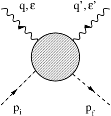
Figure 1: Compton scattering off the pion.

Let us first define the object of interest, namely, the tensor for Compton scattering of off-shell photons (see Fig. 1):

$$(2\pi)^{4}\delta^{4}(p_{f}+q^{\prime}-p_{i}-q)M^{\mu\nu}(p_{f},q^{\prime};p_{i},q)=$$ (1)

$$\int d^{4}x\,d^{4}y\,e^{-iq\cdot x}e^{iq^{\prime}\cdot y}<\!\pi^{\pm}(p_{f})|T[J^{\mu}(x)J^{\nu}(y)]|\pi^{\pm}(p_{i})\!>,$$

where $T$ refers to the covariant time-ordered product. The pions are assumed to be on mass shell. As a special case, the RCS amplitude ($q^{2}=q^{\prime 2}=0$) is obtained by contracting Eq. (1) with the polarization vectors $\epsilon_{\mu}$ and $\epsilon^{\prime\ast}_{\nu}$ of the initial and final photons, respectively,

$${\cal M}=-ie^{2}\epsilon_{\mu}\epsilon^{\prime\ast}_{\nu}M^{\mu\nu}(p_{f},q^{\prime};p_{i},q).$$ (2)

In the laboratory frame ($\vec{p}_{i}=0$), the low-energy expansion of Eq. (2), using Coulomb gauge, reads

$${\cal M}=-2ie^{2}\vec{\epsilon}\,^{\prime\ast}\cdot\vec{\epsilon}+2m_{\pi}i\omega\omega^{\prime}(4\pi\bar{\alpha}\vec{\epsilon}\,^{\prime\ast}\cdot\vec{\epsilon}+4\pi\bar{\beta}\hat{q}\,^{\prime}\times\vec{\epsilon}\,^{\prime\ast}\cdot\hat{q}\times\vec{\epsilon})+\cdots.$$ (3)

The first term is simply the result for a point particle without internal structure and the second term parametrizes the lowest-order response in terms of the electromagnetic polarizabilities $\bar{\alpha}$ and $\bar{\beta}$.

In the framework of classical electrodynamics, the electric polarizability denotes the connection between a uniform static electric field and the induced dipole moment

$$\vec{p}_{ind}=4\pi\alpha\vec{E}.$$ (4)

For instance, the polarizability of a dielectric sphere of radius $R$ and dielectric constant $\epsilon$ is given by $\alpha=\frac{\epsilon-1}{\epsilon+2}R^{3}$. [9]

Figure 2: Dielectric sphere in an external electric field. $\vec{p}_{ind}=4\pi\alpha\vec{E}.$

Using a simple model of a point charge $e$ of mass $m$ bound in a harmonic oscillator potential, the electric polarizability $\alpha=e^{2}/(m\omega^{2})$ is easily seen to be a measure of the stiffness or rigidity of a system [10].

A more general case of Eq. (1), namely $q^{2}<0$ and $q^{\prime 2}=0$, can be studied in the reaction $\pi^{\pm}(p_{i})+e^{-}(k)\to\pi^{\pm}(p_{f})+e^{-}(k^{\prime})+\gamma(q^{\prime})$. We will refer to this situation as virtual Compton Scattering (VCS) because at least one photon is off shell. For example, in the Fermilab SELEX E781 experiment inelastic scattering of high-energy pions off atomic electrons has been measured and data are presently analyzed [11]. At lowest order in the electromagnetic coupling, the relevant diagrams are shown in Fig. 3. In case of the Bethe-Heitler (BH) diagrams (a) and (b), the real photon is emitted by the initial and final electrons. It is straightforward to express this contribution in terms of the electromagnetic form factor of the pion. The interesting VCS process is contained as a building block in diagram (c).

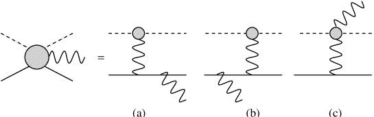
Figure 3: The reaction $\pi^{\pm}(p_{i})+e^{-}(k)\to\pi^{\pm}(p_{f})+e^{-}(k^{\prime})+\gamma(q^{\prime})$ to lowest order in the electromagnetic coupling: Bethe-Heitler diagrams (a) and (b), VCS diagram (c).

Since the invariant amplitude is given by the sum of two contributions ${\cal M}_{BH}$ and ${\cal M}_{VCS}$, the differential cross section is more complicated than in RCS or even in standard electron scattering in the one-photon-exchange approximation:

$$d\sigma\sim|{\cal M}_{BH}+{\cal M}_{VCS}|^{2}.$$

In particular, the four-momenta exchanged by the virtual photons in the BH and VCS diagrams read $r\equiv p_{f}-p_{i}$ and $q\equiv k-k^{\prime}=r+q^{\prime}$, respectively. Unfortunately, the structure-dependent part of the VCS amplitude is only a small contribution of the total amplitude. However, in principle, the different behavior under the substitution $\pi^{-}\to\pi^{+}$ of ${\cal M}_{\mbox{\footnotesize BH}}$ and ${\cal M}_{\mbox{\footnotesize VCS}}$,

$${\cal M}_{\mbox{\footnotesize BH}}(\pi^{-})=-{\cal M}_{\mbox{\footnotesize BH}}(\pi^{+}),\quad{\cal M}_{\mbox{\footnotesize VCS}}(\pi^{-})={\cal M}_{\mbox{\footnotesize VCS}}(\pi^{+}),$$ (5)

could be of use in identifying this contribution by comparing the reactions involving a $\pi^{-}$ and a $\pi^{+}$ beam for the same kinematics:

$$d\sigma(\pi^{+})-d\sigma(\pi^{-})\sim 4\Re\left[{\cal M}_{\mbox{\footnotesize BH}}(\pi^{+}){\cal M}^{\ast}_{\mbox{\footnotesize VCS}}(\pi^{+})\right].$$ (6)

3 Soft-photon amplitude

When studying the low-energy behavior of the VCS amplitude, our first goal is to isolate, in a gauge-invariant fashion, the model-independent part from the total amplitude. The result can be expressed in terms of gross properties of the pion which, in principle, are already known from other experiments. To this end, various methods have been devised in the literature which, up to separately gauge-invariant analytical terms, all give the same result. Here, we will shortly summarize the results of Low’s method [12], where one starts with the amplitude for radiation from “external legs.” This amplitude contains all the contributions which are non-analytic as either $q\rightarrow 0$ or $q^{\prime}\rightarrow 0$. The rationale of this approach is that propagators preceding (following) the emission or absorption of a photon generate the singularities in the soft-photon limit, provided that the particle is on-shell in the final (initial) state. After a thorough expansion of vertices and propagators and dropping analytical terms (see Ref. [5] for details), the result, which we take as $M^{\mu\nu}_{1}$, is

$$M^{\mu\nu}_{1}=F(q^{2})F(q^{\prime 2})\left[\frac{(2p_{i}+q)^{\mu}(2p_{f}+q^{\prime})^{\nu}}{s-m^{2}_{\pi}}+\frac{(2p_{f}-q)^{\mu}(2p_{i}-q^{\prime})^{\nu}}{u-m^{2}_{\pi}}\right],$$ (7)

where $s=(p_{i}+q)^{2}$ and $u=(p_{i}-q^{\prime})^{2}$, and $F$ refers to the electromagnetic form factor of the pion. The next step is to apply the gauge invariance condition to the full amplitude

$${q}_{\mu}M^{\mu\nu}=0,\quad M^{\mu\nu}{q^{\prime}}_{\nu}=0.$$ (8)

From $q_{\mu}M^{\mu\nu}_{1}=2F(q^{2})F(q^{\prime 2})q^{\nu}$ and $M^{\mu\nu}_{1}q^{\prime}_{\nu}=2F(q^{2})F(q^{\prime 2})q^{\prime\mu}$ in combination with Eq. (8) we obtain as a (minimal) solution $M^{\mu\nu}_{2}=-2F(q^{2})F(q^{\prime 2})g^{\mu\nu}$. The resulting soft-photon amplitude (SPA) is then

$$M^{\mu\nu}_{SPA}=F(q^{2})F(q^{\prime 2})\left[\frac{(2p_{i}+q)^{\mu}(2p_{f}+q^{\prime})^{\nu}}{s-m^{2}_{\pi}}+\frac{(2p_{f}-q)^{\mu}(2p_{i}-q^{\prime})^{\nu}}{u-m_{\pi}^{2}}-2g^{\mu\nu}\right].$$ (9)

The total amplitude is given by the soft-photon result of Eq. (9) in combination with a separately gauge-invariant analytical residual amplitude. By construction $M^{\mu\nu}$, $M^{\mu\nu}_{SPA}$, and the residual piece are symmetric with respect to photon crossing $q\leftrightarrow-q^{\prime},\mu\leftrightarrow\nu$ as well as the substitution $p_{i}\leftrightarrow-p_{f}$ (charge conjugation plus particle crossing). For $q^{2}=q^{\prime 2}=0$, Eq. (9) reduces to the result for a structureless spin-zero particle.

4 Generalized dipole polarizabilities

RCS can be described in terms of two functions depending on two scalar variables. We will now discuss a generalization of the RCS polarizabilities to the case $q^{2}\leq 0$ and $q^{\prime 2}=0$. The corresponding invariant amplitude can be parametrized in terms of three functions $B_{1}$, $B_{2}$, $B_{5}$ which depend on three scalar variables [8]:

$$-i{\cal M}=B_{1}F^{\mu\nu}F^{\prime}_{\mu\nu}+\frac{1}{4}B_{2}(P_{\mu}F^{\mu\nu})(P^{\rho}F^{\prime}_{\rho\nu})+\frac{1}{4}B_{5}(P^{\nu}q^{\mu}F_{\mu\nu})(P^{\sigma}q^{\rho}F^{\prime}_{\rho\sigma}).$$ (10)

In Eq. (10) $P=p_{i}+p_{f}$, and $F^{\mu\nu}$ and $F^{\prime}_{\mu\nu}$ refer to the gauge-invariant combinations

$$F^{\mu\nu}=-iq^{\mu}\epsilon^{\nu}+iq^{\nu}\epsilon^{\mu},\quad F^{\prime}_{\mu\nu}=iq^{\prime}_{\mu}\epsilon^{\prime\ast}_{\nu}-iq^{\prime}_{\nu}\epsilon^{\prime\ast}_{\mu}.$$

Eq. (10) becomes particularly simple when evaluated in the pion Breit frame (p.B.f.) defined by $\vec{P}=0$,

$$-i{\cal M}=\left[2B_{1}\vec{B}\cdot\vec{B}^{\prime}-\left(2B_{1}+\frac{P^{2}}{4}B_{2}\right)\vec{E}\cdot\vec{E}^{\prime}+\frac{P^{2}}{4}B_{5}\vec{q}\cdot\vec{E}\vec{q}\cdot\vec{E}^{\prime}\right]_{p.B.f.}.$$ (11)

In order to arrive at this equation, we made use of

$$F^{\mu\nu}F^{\prime}_{\mu\nu} = [-2\vec{E}\cdot\vec{E}^{\prime}+2\vec{B}\cdot\vec{B}^{\prime}]_{p.B.f.},$$

$$P_{\mu}F^{\mu\nu}P^{\rho}F^{\prime}_{\rho\nu} = [-P^{2}_{0}\vec{E}\cdot\vec{E}^{\prime}]_{p.B.f.},$$

$$P^{\nu}q^{\mu}F_{\mu\nu}P^{\rho}q^{\sigma}F^{\prime}_{\sigma\rho} = [P^{2}_{0}\vec{q}\cdot\vec{E}\vec{q}\cdot\vec{E}^{\prime}]_{p.B.f.},$$

where we introduced the notation

$$\vec{E}=i(q_{0}\vec{\epsilon}-\vec{q}\epsilon_{0}),\quad\vec{B}=i\vec{q}\times\vec{\epsilon},\quad\vec{E}^{\prime}=-i(q_{0}^{\prime}\vec{\epsilon}\,^{\prime\ast}-\vec{q}\,^{\prime}\epsilon_{0}^{\prime\ast}),\quad\vec{B}^{\prime}=-i\vec{q}\,^{\prime}\times\vec{\epsilon}\,^{\prime\ast}.$$

Note that by definition $[P^{2}_{0}]_{p.B.f.}=P^{2}$. Finally, decomposing $\vec{E}=\vec{E}_{T}+\vec{E}_{L}$ into components which are orthogonal and parallel to $\hat{q}$, the parametrization of the invariant amplitude in the p.B.f. reads

$$-i{\cal M} = \left\{2B_{1}\vec{B}\cdot\vec{B}^{\prime}-\left(2B_{1}+\frac{P^{2}}{4}B_{2}\right)\vec{E}_{T}\cdot\vec{E}^{\prime}\right.$$ (12)

$$\left.+\left[\frac{P^{2}}{4}B_{5}|\vec{q}|^{2}-\left(2B_{1}+\frac{P^{2}}{4}B_{2}\right)\right]\vec{E}_{L}\cdot\vec{E}^{\prime}\right\}_{p.B.f.}.$$

Eq. (12) serves as the basis of taking the low-energy limit $\omega^{\prime}\to 0$. Discussing only the residual amplitudes, $B_{i}^{r}\to b_{i}^{r}(q^{2})$, it is natural to define the following three generalized dipole polarizabilities

$$8\pi m_{\pi}\beta(q^{2}) \equiv 2b_{1}^{r}(q^{2}),$$ (13)

$$8\pi m_{\pi}\alpha_{T}(q^{2}) \equiv -2b_{1}^{r}(q^{2})-\left(M^{2}-\frac{q^{2}}{4}\right)b_{2}^{r}(q^{2}),$$ (14)

$$8\pi m_{\pi}\alpha_{L}(q^{2}) \equiv -2b_{1}^{r}(q^{2})-\left(M^{2}-\frac{q^{2}}{4}\right)[b_{2}^{r}(q^{2})+q^{2}b_{5}^{r}(q^{2})],$$ (15)

the superscript $r$ referring to the residual amplitudes beyond the soft-photon result. In general, the transverse and longitudinal electric polarizabilities $\alpha_{T}$ and $\alpha_{L}$ will differ by a term, vanishing however in the RCS limit $q^{2}=0$. At $q^{2}=0$, the usual RCS polarizabilities are recovered,

$$\beta(0)=\bar{\beta},\quad\alpha_{L}(0)=\alpha_{T}(0)=\bar{\alpha}.$$ (16)

Observe that $[\vec{B}\cdot\vec{B}^{\prime}]_{p.B.f.}$ and $[\vec{E}_{L}\cdot\vec{E}^{\prime}]_{p.B.f.}$ are of ${\cal O}(\omega^{\prime})$ whereas $[\vec{E}_{T}\cdot\vec{E}^{\prime}]_{p.B.f.}={\cal O}(\omega^{\prime 2})$, since $[\vec{E}_{T}]_{p.B.f}=iq_{0}(\vec{\epsilon}-\vec{\epsilon}\cdot\hat{q}\hat{q})={\cal O}(\omega^{\prime})$. In other words, different powers of $\omega^{\prime}$ have been kept.

5 Results in chiral perturbation theory

5.1 The chiral Lagrangian

Chiral perturbation theory [13, 14] provides a natural basis for discussing low-energy phenomena involving pions, including their interaction with external fields. It is based on a global chiral $\mbox{SU(2)}_{L}\times\mbox{SU(2)}_{R}$ symmetry of QCD in the limit of vanishing $u$- and $d$-quark masses, in combination with the assumption of spontaneous symmetry breaking down to $\mbox{SU(2)}_{V}$. The chiral symmetry of QCD is mapped onto the most general effective Lagrangian in terms of the Goldstone bosons (pions)

$${\cal L}_{\mbox{\footnotesize eff}}={\cal L}_{2}+{\cal L}_{4}+\cdots,$$ (17)

where the subscript $2n$ refers to the order in the so-called momentum expansion. Couplings to external fields, such as the electromagnetic field, as well as explicit symmetry breaking due to the finite quark masses, can be systematically taken into account. Covariant derivatives and quark-mass terms count as ${\cal O}(p)$ and ${\cal O}(p^{2})$, respectively. Weinberg’s power counting scheme allows for a classification of Feynman diagrams by establishing a relation between the momentum expansion and the loop expansion.

The most general chiral Lagrangian at ${\cal O}(p^{2})$ is given by

$${\cal L}_{2}=\frac{F^{2}}{4}\mbox{Tr}\left[D_{\mu}U(D^{\mu}U)^{\dagger}+\chi U^{\dagger}+U\chi^{\dagger}\right],$$ (18)

where $U$ is a unimodular unitary $(2\times 2)$ matrix containing the pion fields. As a parametrization of $U$ we use

$$U(x)=\frac{\sigma(x)+i\vec{\tau}\cdot\vec{\pi}(x)}{F},\quad\sigma^{2}(x)+\vec{\pi}^{2}(x)=F^{2},$$ (19)

where $F$ denotes the pion-decay constant in the chiral limit: $F_{\pi}=F[1+{\cal O}(\hat{m})]=92.4$ MeV. In the isospin-symmetric limit $m_{u}=m_{d}=\hat{m}$, the quark mass is contained in $\chi=2B_{0}\hat{m}=m^{2}_{\pi}$ at ${\cal O}(p^{2})$, where $B_{0}$ is related to the quark condensate $<\!\!\bar{q}q\!\!>$. The covariant derivative $D_{\mu}U=\partial_{\mu}U+\frac{i}{2}eA_{\mu}[\tau_{3},U]$ contains the coupling to the electromagnetic field $A_{\mu}$. The most general structure of ${\cal L}_{4}$ was first obtained by Gasser and Leutwyler (see Eq. (5.5) of Ref. [14]) and contains seven new low-energy constants $l_{i}$,

$${\cal L}_{4} = \cdots+l_{5}\left[\mbox{Tr}(F^{R}_{\mu\nu}UF_{L}^{\mu\nu}U^{\dagger})-\frac{1}{2}\mbox{Tr}(F_{\mu\nu}^{L}F_{L}^{\mu\nu}+F_{\mu\nu}^{R}F_{R}^{\mu\nu})\right]$$ (20)

$$+i\frac{l_{6}}{2}\mbox{Tr}\left(F^{R}_{\mu\nu}D^{\mu}U(D^{\nu}U)^{\dagger}+F^{L}_{\mu\nu}(D^{\mu}U)^{\dagger}D^{\nu}U\right)+\cdots,$$

where $F^{R}_{\mu\nu}=F^{L}_{\mu\nu}=-\frac{e}{2}\tau_{3}(\partial_{\mu}A_{\nu}-\partial_{\nu}A_{\mu})$.

5.2 The soft-photon amplitude

Our goal is to evaluate the VCS amplitude at the one-loop level which corresponds to ${\cal O}(p^{4})$ in the momentum expansion. At ${\cal O}(p^{4})$, the result for the s- and u-channel pole terms reads

$${\cal M}_{P} = -ie^{2}\left\{F(q^{2})\left[\frac{2p_{f}\cdot\epsilon^{\prime\ast}\,(2p_{i}+q)\cdot\epsilon}{s-m_{\pi}^{2}}+\frac{(2p_{f}-q)\cdot\epsilon\,2p_{i}\cdot\epsilon^{\prime\ast}}{u-m_{\pi}^{2}}\right]\right.$$ (21)

$$\left.+2q\cdot\epsilon\,q\cdot\epsilon^{\prime\ast}\frac{1-F(q^{2})}{q^{2}}\right\},$$

where $F(q^{2})$ is the prediction for the pion electromagnetic form factor. In order to obtain Eq. (21), we made use of the electromagnetic vertex at ${\cal O}(p^{4})$

$$\Gamma^{\mu}(p^{\prime},p)=(p^{\prime}+p)^{\mu}F(q^{2})+(p^{\prime}-p)^{\mu}\frac{p^{\prime 2}-p^{2}}{q^{2}}[1-F(q^{2})],\quad q=p^{\prime}-p.$$ (22)

The second part of Eq. (21) is analytical as $q\to 0$ and would have been dropped in the first step of Low’s method. It originates from the term proportional to $q^{\mu}$ in Eq. (22). Observe that Eq. (21) is not gauge invariant.

Figure 4: One-particle-irreducible diagrams. The labels $2n$ in the interaction vertices denote the order of the corresponding Lagrangian. $Z$ is the wave function renormalization constant.

The one-particle-irreducible diagrams of Fig. 4 give rise to a residual part of the form

$${\cal M}_{R}=ie^{2}\left[2\epsilon\cdot\epsilon^{\prime\ast}+2(q^{2}\epsilon\cdot\epsilon^{\prime\ast}-q\cdot\epsilon\,q\cdot\epsilon^{\prime\ast})\frac{F(q^{2})-1}{q^{2}}\right]+\tilde{\cal M}_{R}.$$ (23)

Combining Eqs. (21) and (23), ${\cal M}={\cal M}_{P}+{\cal M}_{R}=\tilde{\cal M}_{P}+\tilde{\cal M}_{R}$, one finds that $\tilde{\cal M}_{P}$ is exactly of the form predicted by Eq. (9) for $q^{\prime 2}=0$. In particular, $\tilde{\cal M}_{P}$ and $\tilde{\cal M}_{R}$ are now separately gauge invariant.

5.3 The residual amplitude

At ${\cal O}(p^{4})$, the result for the residual amplitude $\tilde{\cal M}_{R}$ reads

$$\tilde{\cal M}_{R}=-ie^{2}(q^{\prime}\cdot\epsilon\,q\cdot\epsilon^{\prime\ast}-q\cdot q^{\prime}\epsilon\cdot\epsilon^{\prime\ast})\left[-\frac{4(2l_{5}^{r}-l_{6}^{r})}{F^{2}_{\pi}}+\frac{2q\cdot q^{\prime}-q^{2}}{16\pi^{2}F^{2}_{\pi}q\cdot q^{\prime}}{\cal G}(q^{2},q\cdot q^{\prime})\right],$$ (24)

where ${\cal G}(q^{2},q\cdot q^{\prime})$ is a one-loop function given in Eq. (26) of Ref. [8]. The combination $2l^{r}_{5}-l^{r}_{6}=(2.85\pm 0.42)\times 10^{-3}$ is determined through the decay $\pi^{+}\to e^{+}\nu_{e}\gamma$. Using the results of Sec. 4 it is straightforward to extract the generalized dipole polarizabilities

$$\alpha^{\pi^{\pm}}_{L}(q^{2}) = \alpha^{\pi^{\pm}}_{T}(q^{2})=-\beta^{\pi^{\pm}}(q^{2})$$ (25)

$$= \frac{e^{2}}{8\pi m_{\pi}}\left[\frac{4(2l^{r}_{5}-l^{r}_{6})}{F^{2}_{\pi}}-\frac{q^{2}}{m_{\pi}^{2}}\frac{1}{(4\pi F_{\pi})^{2}}J^{(0)^{\prime}}\left(\frac{q^{2}}{m_{\pi}^{2}}\right)\right],$$

where

$${J^{(0)}}^{\prime}(x)=\frac{1}{x}\left[1-\frac{2}{x\sigma(x)}\ln\left(\frac{\sigma(x)-1}{\sigma(x)+1}\right)\right],\quad\sigma(x)=\sqrt{1-\frac{4}{x}},\quad x\leq 0.$$

The results for the generalized dipole polarizabilities are shown in Fig. 5. The $q^{2}$ dependence does not contain any ${\cal O}(p^{4})$ parameter, i.e., it is entirely given in terms of the pion mass and the pion decay constant $F_{\pi}=92.4$ MeV. At $q^{2}=0$, the electromagnetic polarizabilities of the charged pion are determined by an ${\cal O}(p^{4})$ counter term [10, 15],

$$\bar{\alpha}=-\bar{\beta}=\frac{e^{2}}{4\pi}\frac{2}{m_{\pi}F^{2}_{\pi}}(2l^{r}_{5}-l^{r}_{6})=(2.68\pm 0.42)\times 10^{-4}\,\mbox{fm}^{3}.$$ (26)

Corrections to this result at ${\cal O}(p^{6})$ were shown to be reasonably small, namely 12% and 24% of the ${\cal O}(p^{4})$ values for $\bar{\alpha}$ and $\bar{\beta}$, respectively [16]. Empirical results for the RCS polarizabilities have been obtained from high-energy pion-nucleus bremsstrahlung, $\bar{\alpha}_{\pi\pm}=(6.8\pm 1.4)\times 10^{-4}\,\mbox{fm}^{3}$ [17], $\bar{\beta}_{\pi^{\pm}}=(-7.1\pm 4.6)\times 10^{-4}\,\mbox{fm}^{3}$ [18], and radiative pion photoproduction off the nucleon, $\bar{\alpha}_{\pi\pm}=(20\pm 12)\times 10^{-4}\,\mbox{fm}^{3}$ [19]. An improved accuracy is required to test the chiral predictions.

As in the case of RCS, we expect the degeneracy $\alpha_{L}(q^{2})=\alpha_{T}(q^{2})=-\beta(q^{2})$ to be lifted at the two-loop level.

Figure 5: ${\cal O}(p^{4})$ prediction for the generalized dipole polarizabilities $\alpha_{L}(-Q^{2})$ of the charged pion (solid curve) and the neutral pion (dashed curve) as function of $Q^{2}$. At ${\cal O}(p^{4})$, $\alpha_{L}(q^{2})=\alpha_{T}(q^{2})=-\beta(q^{2})$.

6 Summary

We discussed the invariant amplitude for virtual Compton scattering off the charged pion $\gamma^{\ast}+\pi\to\gamma+\pi$ which enters the reaction $\pi+e\to\pi+e+\gamma$. In the framework of Low’s method we derived the soft-photon result which depends only on the electromagnetic form factor of the pion. From the analysis of a covariant approach, evaluated in the pion Breit frame, we introduced three generalized dipole polarizabilities which are functions of the squared virtual-photon momentum transfer.

We then discussed VCS of the pion in the framework of ChPT at ${\cal O}(p^{4})$. As expected, the ChPT result reproduces the soft-photon amplitude. The momentum dependence of the generalized polarizabilities is entirely predicted in terms of the pion mass and the pion-decay constant, i.e., no additional counter-term contribution appears. The predictions at ${\cal O}(p^{4})$ show a degeneracy of the polarizabilities, $\alpha_{L}(q^{2})=\alpha_{T}(q^{2})=-\beta(q^{2})$. As in the case of real Compton scattering, we expect the degeneracy to be removed at the two-loop level.

References

• [1] F.E. Low, Phys. Rev. 96, 1428 (1954).
• [2] M. Gell-Mann and M.L. Goldberger, Phys. Rev. 96, 1433 (1954).
• [3] A. Klein, Phys. Rev. 99, 998 (1955).
• [4] S. Scherer, A.Yu. Korchin, and J.H. Koch, Phys. Rev. C 54, 904 (1996).
• [5] H.W. Fearing and S. Scherer, Few-Body Syst. 23, 111 (1998).
• [6] P.A.M. Guichon, G.Q. Liu, and A.W. Thomas, Nucl. Phys. A591, 606 (1995).
• [7] D. Drechsel, G. Knöchlein, A. Metz, and S. Scherer, Phys. Rev. C 55, 424 (1997).
• [8] C. Unkmeir, S. Scherer, A.I. L’vov, and D. Drechsel, hep-ph/9904442.
• [9] J.D. Jackson, Classical Electrodynamics (John Wiley, New York, 1975) Sect. 4.4.
• [10] B.R. Holstein, Comments Nucl. Part. Phys. 19, 221 (1990).
• [11] M.A. Moinester et al. (The SELEX Collaboration), hep-ex/9903039.
• [12] F.E. Low, Phys. Rev. 110, 974 (1958).
• [13] S. Weinberg, Physica 96A, 327 (1979).
• [14] J. Gasser and H. Leutwyler, Ann. Phys. (N.Y.) 158, 142 (1984).
• [15] M. V. Terent’ev, Sov. J. Nucl. Phys. 16, 87 (1973).
• [16] U. Bürgi, Phys. Lett. B 377, 147 (1996); Nucl. Phys. B479, 392 (1996).
• [17] Yu.M. Antipov et al., Phys. Lett. 121B, 445 (1983).
• [18] Yu.M. Antipov et al., Z. Phys. C 26, 495 (1985).
• [19] T.A. Aibergenov et al., Czech. J. Phys. B36, 948 (1986).