A 3–Dimensional Calculation of
Atmospheric Neutrino Flux

Abstract

An extensive 3-dimensional Monte Carlo calculation of the atmospheric neutrino flux is in progress with the FLUKA Monte Carlo code. The results are compared to those obtained under the 1-dimensional approximation, where secondary particles and decay products are assumed to be collinear to the primary cosmic ray, as usually done in most of the already existing flux calculations. It is shown that the collinear approximation gives rise to a wrong angular distribution of neutrinos, essentially in the Sub-GeV region. However, the angular smearing introduced by the experimental inability of detecting recoils in neutrino interactions with nuclei is large enough to wash out, in practice, most of the differences between 3–dimensional and 1–dimensional flux calculations. Therefore, the use of the collinear approximation should have not introduced a significant bias in the determination of the flavor oscillation parameters in current experiments.

1 Introduction

The recent experimental observations concerning atmospheric neutrinos in SuperKamiokande [1], Soudan2 [2] and MACRO [3], have given new strength to the hypothesis of the existence of non zero neutrino masses and of flavor neutrino mixing.

The precise determination of the oscillation mechanism and of the oscillation parameters is, and will be in the next years, still object of intensive work. Even in view of future experimental activities with long–baseline neutrino beams from accelerators, atmospheric neutrino experiments are going to play a fundamental role. In all cases, the optimization of the detectors must be accompanied by an improvement of the precision of theoretical prediction both for the fluxes and for neutrino interactions. Indeed, the determination of the allowed and excluded regions in the oscillation parameter space for all experiments are heavily relying on the comparison of experimental data to Monte Carlo predictions. In this respect, one of the most important inputs is the deviation of the zenith angle distribution of upward going $\nu_{\mu}$’s with respect to the expectation, as observed by SuperKamiokande. In particular, one of the main new experimental findings of SuperKamiokande, when compared to the previous experiments, is the observation of an angular modulation of both the Sub-GeV and Multi-GeV muon neutrino (and antineutrino) samples, while in the progenitor detectors like Kamiokande [4] or IMB [5], apart from considerations concerning the statistical significance, only the Multi-GeV sample deviated from expectation. For both the experiments at Kamioka, the expectation is calculated using the simulation by Honda et al. [6]. Other experiments, like Soudan2 and MACRO, mostly refer to the predictions based on the Bartol Monte Carlo [7].

These two simulations have been performed by means of different shower codes with different hadronic interaction models and different input spectra for the primary cosmic rays. The importance of these two aspects for the evaluation of the systematic uncertainty of neutrino fluxes is still a matter of debate. Here, we want to focus the discussion on another aspect of existing calculations which in principle might be relevant for the angular distribution at low energies, and therefore for the determination of the value of oscillation parameters. As a matter of fact, a common feature of both the Bartol and Honda simulations (and in those of other authors), is the assumption that the neutrino fluxes can be calculated using a 1–dimensional approach. This approximation in practice implies that the transverse momentum of secondary particles after an interaction or decay can be neglected, so that all secondary mesons and eventually their decay products, neutrinos included, are collinear with the parent cosmic ray particles. The argument invoked to justify this approach is that all possible effects deriving from the choice of this approximation, if any, are small and are compensated, in average, by the fact that primary cosmic rays arrive from every direction, and therefore a 3-dimensional calculation can contribute only to establish second order effects, not essential for the understanding of the relevant physics underneath. The average angle between the direction of a neutrino from pion decay, for instance, and the direction of the primary is expected to be:

$$<\theta_{N\nu}>\simeq\frac{<P^{\pi}_{\perp}>}{P_{\pi}}\simeq\frac{0.3~{}GeV}{4E_{\nu}}=\frac{4.3^{\circ}}{E_{\nu}(GeV)}$$ (1)

The $\pi\nu$ angle can be considered a minor correction. In the case of $\nu$’s from $\mu$ decay, an additional contribution comes from the deviation of $\mu^{\pm}$ in the geomagnetic field. We expect this to be small, and, in first approximation, independent of energy, since the flight path of low energy muons and their curvature radius identically scale with $P_{\mu}$.

In view of the improvement in the quality and precision of predictions for future generation experiments, as Icarus at Gran Sasso [8], a new full 3-Dimensional calculation, including also the spherical representation of the atmosphere and of the Earth, has been started. It is based on the FLUKA Monte Carlo [10], which is a highly detailed and precise code for the study of transport and interaction of particles in matter, and in particular for e.m. and hadronic shower simulations. The work is still in progress. Preliminary results were already presented in [9]. Here we want to show that important differences exist, in principle, in the angular distribution of low energy neutrinos when 3–Dimensional and collinear calculations are compared. The collinear approach is justified only above a certain energy range. This is a conclusion which holds irrespectively of all the other main ingredients of shower simulation: primary spectra, geomagnetic field, hadronic interactions,etc. The impact on the physics analysis of neglecting the 3–Dimensional effects depend also on the physics of neutrino interactions and on the resolution of a specific detector in the reconstruction of neutrino direction.

In the following, we shall first summarize the main features of the simulation set up, then we shall discuss the simulation results. These will be presented comparing the angular distribution in the full 3–D approach to that obtained in the collinear one. We remark that the results presented here do not yet include a discussion of the absolute values of neutrino fluxes coming from this new calculation. As a further point, we shall consider the features of neutrino charged current interactions in order to understand the smearing effect introduced. We shall attempt some considerations about the relevance of the 3–D effects for high resolution experiments. The questions concerning possible differences due to the combined effect of geomagnetic cutoff are also briefly reviewed. The qualitative differences in the results between the 3–D and 1–D approach can be understood using an analytical approach: this is shown in a final Appendix.

2 The Simulation Set–up

The FLUKA code [10] is a general purpose Monte Carlo code for the interaction and transport of particles. It is built and maintained with the aim of including the best possible physical models in terms of completeness and precision. Therefore it contains very detailed models of electromagnetic, hadron–hadron and hadron–nucleus interactions, covering the range from the MeV scale to the many–TeV one. Extensive benchmarking against experimental data has been produced (see the references in [10]). In view of applications for cosmic ray physics, we have implemented a 3–Dimensional spherical representation of the whole Earth and of the surrounding atmosphere. This is described by a medium composed by a proper mixture of N, O and Ar, arranged in 51 concentric spherical shells, each one having a density scaling according to the known profile of “standard atmosphere” [11]. Primary particles, sampled from a continuous spectrum, are injected at the top of the atmosphere, at about 100 km of altitude. The primary flux is assumed to be uniform and isotropic. The flux of all possible secondary products are scored at different heights in the atmosphere and at the Earth boundary. Therefore, we are able to get, besides neutrino fluxes, the flux of muons and hadrons to be used for the benchmarking against existing experimental data. All relevant physics, such as energy loss, transport in magnetic field, polarized decay, etc are included in the code by default, and different geomagnetic models can be considered. As mentioned before, the discussion on the full calculation of neutrino fluxes would need an accurate examination of all the mentioned ingredients of the code. All this is postponed to another paper, since this is not relevant for the purpose of this work. We limit ourselves to address the reader to the quoted references, and to mention that we made use of the same primary all–nucleon spectrum used by the Bartol group, as in [12]. The geomagnetic cutoff is applied a posteriori. Therefore in the first stage the calculation exploits the spherical symmetry of the geometry and of the primary flux: all points of the sphere surface are equivalent and can be used to score the neutrino flux. This symmetry, in realistic conditions, is broken mostly by the effects of geomagnetic field. In the following, for sake of clarity, we shall discuss mainly the angular distribution for the symmetric flux. Further effects after the inclusion of geomagnetic cutoff are mentioned in the last section.

We can introduce the main topic of this work by showing a first output from the full simulation, that is the distribution of the angle between a neutrino crossing the Earth’s surface and the primary nucleon direction, as that of Fig. 1 a) and b) for muon and electron neutrino respectively, where different intervals of neutrino energy are considered separately. These distributions have been obtained integrating on the whole energy spectrum and angular distribution of primaries.

Figure 1: Calculated distribution of $\theta_{N\nu}$ (degrees) in different neutrino energy bins. Up: muon neutrinos. Down: electron neutrinos.

From these plots, and from the average values reported in Table 1, we immediately notice the following features:

1. While in the Multi-GeV region that the collinear approximation is reasonable, in the Sub-GeV region the average angle with respect to the primary direction is quite large, in substantial agreement with the expectation from eq.1

2. At very low energies, the average $\theta_{N\nu}$ is somewhat larger for electron neutrinos, as also summarized in Table 1. This is due to the fact that, in average, electron neutrinos come from a later stage of the decay chain.

Energy range (GeV)	$<\theta_{N\nu}>$ (degrees)
	$\nu_{\mu}+\overline{\nu}_{\mu}$	$\nu_{e}+\overline{\nu}_{e}$
0.0 - 0.25	47.6	53.4
0.25 - 0.5	23.8	27.6
0.5 - 1.0	15.6	15.9
1.0 - 2.0	8.9	9.0
2.0 - 5.0	4.4	4.6
5.0 - 20.0	1.8	1.8
20.0 - 200.0	0.5	0.5

Table 1: Average $\theta_{N\nu}$ (angle with respect to primary particle) for different neutrino flavors and energy intervals.

3 Simulation Results

We have performed two different kinds of simulation runs. The first one exploits all the features of the simulation code. In the second run we have repeated the simulation forcing the collinear approach. At each interaction or decay, the angle of secondary particles with respect to the primary direction has been set to the null value. Furthermore, following a recipe in use in the Bartol calculations [13], all (low energy) neutrinos emitted at more than 90^∘ with respect to the primary direction in the laboratory frame have been disregarded.

Before showing the results of numerical simulations, we want to remark the existence of an effect on the flux normalization as a function of angle and energy. This can be understood following the analytical considerations reported in the Appendix. We also notice that for trajectories close to the horizontal direction with respect to a given position on the sphere, there will be cases in which, if perfect collinearity is assumed, no neutrino will ever touch the Earth surface but they will all escape through the atmosphere. In the 3–Dimensional case, thanks to a possible large $\theta_{N\nu}$, some neutrinos can instead be intercepted.

3.1 Neutrino Flux and Angular Distribution

Fig.2 shows the $cos\theta$ distribution ($\theta$ is the zenith angle) of $\nu_{\mu}$ for 4 different energy regions, for the 3-Dimensional and the collinear approach. Fig. 3 is the analogous plot for $\nu_{e}$. Similar plots are obtained for anti–neutrinos. These results confirm that in the Sub–GeV range, when the average $\theta_{N\nu}$ is large, there are important differences between the two approaches. The 3-Dimensional calculation predicts an anisotropic angular distribution, with an enhancement in the horizontal direction, as qualitatively expected by the analytical arguments which are reported in the Appendix. Conversely, the 1-D results give a substantially flat distribution. We remind that the geomagnetic cut–off has not yet been applied to the calculated fluxes and perfect spherical symmetry holds.

Figure 2: Comparison of the $cos(Zenith)$ dependence of $\nu_{\mu}$ flux in 4 different energy regions, for the 3-Dimensional and the collinear (1-D) approach, as obtained in the FLUKA simulation with spherical geometry.

Figure 3: Comparison of $cos(Zenith)$ dependence of $\nu_{e}$ flux in 4 different energy regions, for the 3-Dimensional and the collinear (1-D) approach, as obtained in the FLUKA simulation with spherical geometry.

Other important differences are visible in the distribution of production height of neutrinos, again only in the low energy range, where the distribution is broader in the 3–D case than in the 1–D case. This is particularly evident around the horizontal direction (see Fig. 4 and Fig. 5).

As far as the normalization of the integrated flux is concerned, a small excess is obtained at low energy, as shown in Fig. 6.

Figure 4: Distribution of production height of Sub–GeV (up) and Multi–GeV $\nu_{\mu}$ and $\overline{\nu}_{\nu}$ around the horizontal ($|cos\theta|<0.2$) as obtained with FLUKA, comparing 3–D and 1–D simulations.

Figure 5: Distribution of production height of Sub–GeV (up) and Multi–GeV $\nu_{e}$ and $\overline{\nu}_{e}$ around the horizontal ($|cos\theta|<0.2$) as obtained with FLUKA, comparing 3–D and 1–D simulations.

Figure 6: Comparison of angular integrated flux for different $\nu$ flavors for the 3-Dimensional and the collinear (1-D) approach, as obtained in the FLUKA simulation with spherical geometry, for a generic point on the Earth surface (no geomagnetic cutoff is applied).

3.2 Detected Neutrinos and Reconstructed Direction

We can distinguish between the flux of neutrinos, and its angular distribution on one side, and, on the other, the rate of neutrino interactions (typically of the charged current type) with their reconstructed direction distribution. Since we have already stated that the Sub–GeV neutrinos as the critical ones, we shall restrict to this range the discussion. In this energy range, nuclear effects play an important role in modifying the kinematics of neutrino interactions with respect to the free nucleon case. The impact on the event reconstruction is not at all negligible and depends on the detector characteristics. The rate of low energy $\nu_{\mu}$ and $\nu_{e}$ CC interactions is largely dominated by quasi–elastic scattering. The outgoing lepton direction is often assumed to be a good approximation of the incident neutrino direction. It is fundamental to consider the neutrino interaction in the nuclear environment. Modifications of the $Q^{2}$ distributions are expected due to Pauli blocking and threshold effects. In quasi-elastic scattering, the average $Q^{2}$ for a 1 GeV $\nu_{\mu}$ ($\overline{\nu}_{\mu}$) is about $0.4$ ($0.2$) GeV²/c²; at 300 MeV these average values drop to $\sim 0.10$ ($0.06$) GeV²/c². At these energies and above, the approximation of independent nucleons in a potential well can be used, since $Q^{2}/2m\buildrel>\over{{}_{\sim}}0.030$ GeV, the typical kinetic energy of a bound nucleon. The Fermi momentum of the struck nucleon adds a smearing to the lepton angular distribution and to the momentum of the lepton-nucleon system, that is balanced by the momentum of the nuclear recoil. Moreover, the struck nucleon can re–interact in the nuclear medium, with changes in the energy, number and identity of reaction products. The residual nucleus is generally left in an excited state, due to the removal of deeply bound nucleons and to the differences in binding energy: this excitation energy is dissipated through particle evaporation and gamma ray emission. The overall momentum and energy are of course conserved, but they can be exactly reconstructed only by detecting all reaction products, including the recoil nucleus, all the low energy evaporation products (often neutrons) and gamma rays from nuclear de–excitation. The inaccuracies in the event reconstruction lead to a smearing of the reconstructed neutrino angular distribution, that could partially obscure the differences between the 3-D and 1-D case. To evaluate the effect under several “experimental” conditions, charged current neutrino interactions in Argon have been simulated starting from the 3-D and 1-D calculated flux. This was done in the framework of the same modelling tool, since the FLUKA MC code now includes the description of neutrino–nucleus interactions [14, 15], fully embedded in the FLUKA nuclear interaction model. For quasi–elastic interactions, the model of [16] for $\nu$–N interactions has been followed. Details of this implementation and of the FLUKA code can be found elsewhere[14, 10, 17]. We only remind remark here that it is a sophisticated intranuclear cascade plus pre–equilibrium code, which is very successful in reproducing low energy phenomenology in hadron-nucleus collisions[10].

The simulated events have been used to reconstruct the neutrino angular distribution, under different assumptions. Let us start considering the case in which only the outgoing lepton is measured, as in SuperKamiokande selection of single ring events. Fig. 7 shows the angular distribution of Sub–GeV muon neutrinos undergoing CC interactions, when no flavor oscillations are considered, in the 3–D (a) and 1–D (b) approaches. The simulated sample corresponds to an exposure of 1000 kton$\cdot$yr. No detector resolution has been considered and we remind that no geomagnetic cutoff has been yet introduced. In (c) and (d) we show the reconstructed angular distribution when the direction of neutrinos is assumed to be that of detected muon. We can notice that the smearing of the $\nu-\mu$ angle is large enough to wash out almost all the differences between 3–D and 1–D simulations.

Figure 7: Zenith angular distribution for CC–interacted $\nu_{\mu}$ events (E${}_{\mu}<$ 1.33 GeV) in four cases: a) true neutrino angle (3–D simulation) b) true neutrino angle (1–D simulation) c) using only lepton reconstruction (3–D simulation) d) using only lepton reconstruction (1–D simulation) The statistical sample corresponds to an exposure of 1000 kton$\cdot$yr. No geomagnetic cutoff is applied and no detector resolution is considered.

This is still valid even in presence of factors, like flavor oscillations, distorting the neutrino angle distribution. This is visible in Fig. 8 where the 4 cases of Fig. 7 are shown for a maximal mixing $\nu_{\mu}$ disappearance due to flavor oscillation with $\Delta m^{2}=5\cdot 10^{-3}eV^{2}$ As expected, when instead Multi-GeV events are selected, no real difference exists between the 3–D and 1–D predictions even when the true neutrino angle is considered.

Figure 8: Same as fig. 7, when maximal mixing $\nu_{\mu}$ oscillation is introduced, for $\Delta m^{2}$ = 5$\cdot$ 10^-3 eV². a) true neutrino angle (3–D simulation) b) true neutrino angle (1–D simulation) c) using only lepton reconstruction (3–D simulation) d) using only lepton reconstruction (1–D simulation)

The additional information carried by charged particles produced in neutrino scattering, which can be identified in detectors with higher resolution than SuperKamiokande, has been considered as a tool to improve the direction resolution [18]. However, the smearing introduced by the nuclear effects results to be still large enough to obscure the 3–D effects. We have also investigated the possible additional benefits coming from the detection of low energy evaporation products (mainly neutrons), although these are expected to be isotropically distributed. The only way to recover the correct distribution would be to measure the momentum of the recoiling nucleus, which is unfortunately not possible, even in very high resolution detectors.

The results are reported in Fig. 9, where the reconstructed angular distribution of $\nu_{\mu}+\overline{\nu}_{\mu}$ neutrinos (no oscillations) is shown for the 3–D simulation only, comparing three different cases: i) when the charged lepton and hadrons are measured, ii) when also evaporation neutrons are added; iii) when only the lepton is reconstructed. We are still assuming the ideal case of perfect energy and direction resolution for the detected particles. The true 3–D angular distribution is also shown for comparison. Some improvement can be noticed when charged hadrons are considered. The addition of neutrons does not give a significant improvement. Some advantage comes from the fast neutrons which are produced in nuclear re–scattering, but they are very few.

Figure 9: Reconstructed zenith angular distribution for CC $\nu_{\mu}+\overline{\nu}_{\mu}$ interactions (E${}_{\mu}<$ 1.33 GeV, 1000 kton$\cdot$yr exposure) in three cases: a) when the direction reconstruction is given by the combination of the reconstruction of the muon and of the possible charged hadrons; b) when also the neutrons from nuclear de-excitation are included. c) when only the muon is measured. For reference, the true angular distribution are also shown.

The same cases of Fig.9 are repeated in Fig.10 when maximal mixing $\nu_{\mu}$ oscillations are introduced with $\Delta m^{2}$ = 5$\cdot$10^-3 eV².

Figure 10: Reconstructed zenith angular distribution for CC $\nu_{\mu}+\overline{\nu}_{\mu}$ interactions (E${}_{\mu}<$ 1.33 GeV, 1000 kton$\cdot$yr exposure) in the same cases of Fig.9 for maximal mixing oscillations with $\Delta m^{2}$ = 5$\cdot$10^-3 eV².

As a final exercise on this topic, we looked at the muon neutrino oscillation pattern, following the analysis method described in [19, 20]. The number of events is plotted as function of L/E, where L is the estimated path of neutrino from production to detection and E is the neutrino energy. In Fig.11 we show the ratio of the L/E distribution of simulated $\nu_{\mu}+\overline{\nu}_{\mu}$ events in the case of maximal mixing oscillations and $\Delta m^{2}$ = 5$\cdot$10^-3 eV² to that of the same sample when no oscillation are present, for different event reconstructions. Once again the simulated statistics corresponds to an exposure of 1000 kton$\cdot$yr (3–D simulation) and no experimental resolution is applied. The statements concerning the importance of the recoil of the nucleus are confirmed: the oscillation pattern is totally hindered when the lepton alone is detected, and is strongly suppressed unless the event is fully reconstructed. Of course, if high energy events are selected (typically when $P_{\mu}>$ 1$\div$2 GeV), the oscillation pattern can be recovered even with the muon reconstruction alone.

Figure 11: Ratio of the L/E distribution of simulated $\nu_{\mu}+\overline{\nu}_{\mu}$ events in the case of maximal mixing oscillations and $\Delta m^{2}$ = 5$\cdot$10^-3 eV² to that of the same sample when no oscillations are present, for different event reconstructions, CC $\nu$ interactions are selected.

4 Inclusion of Geomagnetic Cutoff

Further differences between the 3–D and 1–D calculations could be expected in principle when geomagnetic cutoffs are applied to the primary nucleons and nuclei. Technically, this is usually accomplished applying a rejection algorithm to the unperturbed flux. It depends on the geomagnetic location of the detector, on the geomagnetic location and altitude of primary interaction, primary rigidity and on the zenith and azimuth angles of the arrival direction of primary. In the collinear approximation, the coordinates and arrival direction of primary are instead strictly linked to those of the neutrino. We might expect, in principle, a different result in the energy-angle correlation, again for Sub–GeV neutrinos. In order to check this, we introduced the geomagnetic cutoff in our simulation runs, both 3–D and 1–D, by means of the technique of anti–proton back–tracing, expressing the geomagnetic field as an expansion in spherical harmonics, similar to that described in the work of Honda et al. [6]. This has been done for different geographical sites. Similar results have been obtained with a faster algorithm, in which the geomagnetic field is described by a dipole properly off-centered with respect to the Earth sphere [21]. As an example, in Fig. 12 we show the neutrino flux at low energy for different flavors as a function of $cos\theta$ in the site of SuperKamiokande, comparing the 3–D and 1–D results.

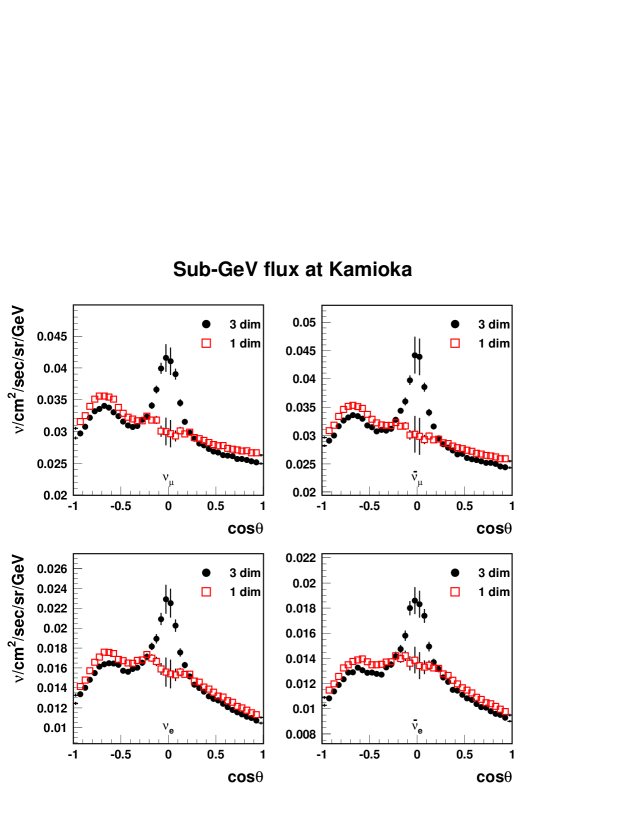
Figure 12: Neutrino flux as a function of Zenith angle, for the different flavors, as predicted for the site of SuperKamiokande. Results from 3–D and 1–D simulations are compared.

The up–down differences are now visible. The enhancement around the horizontal direction for the 3–D simulation remains visible, but it will be smeared after neutrino detection. In order to show this, we have calculated the up–down asymmetry parameter for Sub-GeV muon neutrinos under the hypothesis of a maximal mixing oscillation into an undetected flavour, as a function of $\Delta m^{2}$. In order to make a realistic exercise, we have introduced selections similar to those adopted in the recent SuperKamiokande analyses [22], i.e. using the muon direction, excluding a region around the horizontal ($|cos\theta|\leq$ 0.2) and accepting lepton momenta above 0.4 GeV/c. The result is shown in in the upper part of Fig. 13. The 3–D and 1–D approaches are identified by different line styles. The expected uncertainty region of SuperKamiokande after the analysis of the 45 kton exposure sample is reported [22] (we considered the statistical error and the quoted 5% systematic error added in quadrature). Differences exist, but they are again small. Once again, the smearing in the reconstructed angle introduced by neutrino interactions obscures the effect. In the bottom part of the same figure we show what would be obtained if the true neutrino direction could be recovered. Even in this hypothetical case, the differences comparing 3–D are 1–D are too small.

Figure 13: Simulation of the asymmetry parameter for $\nu_{\mu}$+$\overline{\nu}_{\mu}$ in case of maximal mixing oscillation, as a function of $\Delta m^{2}$, for the Sub-GeV events in SuperKamiokande. Upper panel: using reconstructed neutrino direction for single ring events. Lower panel: the same result assuming that the true neutrino direction is know. The continuous (dotted) line is the prediction from the 3–D (1–D) simulation. The band relative to the total uncertainty of SuperKamiokande after 45 kton$\cdot$yr is also shown.

The East-West effect has been also considered, but again no noticeable difference has been detected between the 3–D and 1–D approaches, as shown in Fig. 14, where the situation of SuperKamiokande (without oscillations) has been simulated, using the same selection cuts described in [23].

A posteriori, these results are not surprising. As we have shown in the plots when no cutoff was yet introduced, the 3–D effects introduce an enhancement around the horizontal direction, but with a perfect up–down symmetry. The small differences that can be noticed in Figg. 13 and 14 are essentially due to oscillation effects coming from differences in the path lengths of neutrinos.

Figure 14: Simulation of the east-west effect (without oscillation) for the SuperKamiokande site for the two neutrino flavors. The 3–D and 1–D simulation in the spherical geometry are compared.

5 Conclusions

We have shown that the collinear approximation that has been used for many evaluations of atmospheric neutrino fluxes is based upon a wrong assumption and leads to an incorrect angular distribution of neutrinos at the Earth’s surface. This turns out to be relevant for Sub-GeV energy range. However, a precise experimental momentum reconstruction is hardly achievable due to the the features of neutrino-nucleus charged current interaction at low energies. In realistic situations, this induces a the smearing on the measured angular distribution that is such to obscure in great part the differences with respect to a full 3–D simulation. This is true not only when just the outgoing lepton is measured, as in the single ring events of SuperKamiokande, but also when the recoiling nucleon is measured as well, provided that the residual recoiling nucleus is undetected. In summary, the consequences for physics analyses following from the use of the collinear approximation in the flux calculation are very small. In particular, referring to the question of neutrino flavor oscillations, the limits on $\Delta m^{2}$ affected by the angular distribution of Sub-GeV neutrinos, should remain practically unchanged. Nevertheless, experimental analysis aiming to achieve the maximum possible precision should make use of a full 3–D simulation in spherical geometry. There are other experimental observables which could be more directly affected by the 3–D features. For example, the measurement of the low energy muon flux in the high atmosphere is often considered an important benchmark for the Monte Carlo codes for atmospheric neutrinos. We expect that the agreement of existing calculations with the present data might be improved considering the 3–D simulation, and in this case there is no intermediate smearing as that emerging from neutrino–nucleus interaction. Again, we expect the differences to show up preferentially around the horizontal direction, but the existing measurements were all performed around the vertical. Possibly, new experiments could consider the possibility of increasing the angular acceptance of the detector.

Appendix: An attempt of analytical description

The assumption at the basis of the collinear approximation is just that the effects of $\theta_{N\nu}$ are cancelled once that the primary particles are isotropically distributed. Such hypothesis is in principle wrong, and before entering in the examination of the calculation results, it can be instructive to consider a simple case, that can be analytically described, which demonstrates that.

It is the case of a planar geometry, in which an isotropic flux of primary particles $\phi_{0}$ fills half the space (the region $z<0$). The plane $z=0$ acts as a perfect absorber: all primary particles that touch the plane are absorbed and during this process each one of these particle emits an average number of neutrinos $\langle n_{\nu}\rangle$. The capture rate $C$ (the number of primary particle captures per unit time and unit surface) is easily calculated as:

$$C=2\pi\,\int_{0}^{1}dx~{}x\,\phi_{0}=\pi\;\phi_{0}$$ (2)

where we have assumed that all primary particle are ultrarelativistic, set the speed of light to $c=1$, and defined $x=\cos\theta_{0}$ as the component of the velocity of the primary particle orthogonal to the absorbing plane ($x=1$ corresponds to a particle moving orthogonally and toward the plane). Obviously the rate of absorption is linear in $x$. The absorbing plane is a source of neutrinos. Integrating over all emission angles the number of neutrinos emitted per unit time and unit of surface is obviously:

$$S_{\nu}=C~{}\langle n_{\nu}\rangle=\pi\,\phi_{0}\,\langle n_{\nu}\rangle.$$ (3)

We are interested in the angular distribution of the emitted neutrinos $dS_{\nu}/dy$ where $y=\cos\theta_{\nu}$ is the component of neutrino direction orthogonal to the absorbing plane. We can write in general:

$${dS_{\nu}\over dy}=\pi\;\phi_{0}\langle n_{\nu}\rangle\;f(y)$$ (4)

where the function $f(y)$ satisfies the normalization condition

$$\int_{-1}^{+1}dy~{}f(y)=1.$$ (5)

To compute the form of $f(y)$ we need to specify the angular distribution of the neutrinos with respect to the primary particle direction. Two limiting cases are easy to obtain. In the case where the neutrinos are emitted isotropically we have $f_{iso}(y)={1\over 2}$. In the case where the neutrinos are exactly collinear to the primary particle direction we have $f_{coll}(y)=2y~{}\theta(y)$, where the function $\theta$ is defined as: $\theta(x)=0$ for $x<0$ and $\theta(x)=1$ for $x\geq 0$.

In order to solve the most general case of an arbitrary angular distribution we can solve the special problem where the neutrinos is emitted at a fixed angle $\alpha$ with respect to the primary direction (with an additional azimuthal angle $\beta$ uniformly distributed between 0 and $2\pi$. The case of an arbitrary distribution of primary–neutrino angle can then be obtained with a simple integration.

The source of neutrinos in a given direction can be obtained summing over all appropriate combinations of primary direction and azimuthal emission angle:

$$f_{\alpha}(y)=~{}2\,\int_{0}^{1}dx~{}x~{}\int_{0}^{2\pi}{d\beta\over 2\pi}~{}\delta[y-(x\,\cos\alpha-\sqrt{1-x^{2}}\,\sin\alpha\,\cos\beta)]$$ (6)

The result of the integration is:

$$f_{\alpha}(y)=\cases{0,&for $y<-\sin\alpha$ and $\cos\alpha>0$\cr&or $y>\sin\alpha$ and $\cos\alpha<0$,\cr 2\,\cos\alpha\,y,&for $y>\sin\alpha$ and $\cos\alpha>0$\cr&or $y<-\sin\alpha$ and $\cos\alpha<0$,\cr F_{\alpha}(y)&otherwise.}$$ (7)

with

$$F_{\alpha}(y)=\cos\alpha\;y+{2\over\pi}\sqrt{1-\cos^{2}\alpha-y^{2}}-{2\over\pi}\cos\alpha\;y~{}\tan^{-1}\left[{\cos\alpha\;y\;\sqrt{1-\cos^{2}\alpha-y^{2}}\over\cos^{2}\alpha+y^{2}-1}\right]$$ (8)

The resulting angular distribution is therefore different from the collinear expectation. This is recovered in the limit of $\alpha\to 0$, where we have $f_{\alpha}(y)\to 2y\;\theta(y)$. Averaging over all emissions angles we also find:

$$\int_{-1}^{+1}d\cos\alpha~{}f_{\alpha}={1\over 2}$$ (9)

as expected for an isotropic distribution. Note that in general we can distinguish three different angular regions for the emission of the neutrinos. In the case $\alpha<{\pi\over 2}$ we have that no neutrinos are emitted in the most backward directions ($y<-\sin\alpha$). For the most forward directions $y>\sin\alpha$ the angular distribution has the same linear form of the collinear case but the normalization is suppressed : $f_{\alpha}(y)=\cos\alpha\ y$. In the intermediate region $-\sin\alpha\leq y\leq\sin\alpha$ one has a more complex behaviour. The case $\alpha\geq{\pi\over 2}$ can be obtained from the previous case with a reflection, that is with the substitutions $\cos\alpha\to-\cos\alpha$, $y\to-y$.

These analytical consideration can be extended to the spherical geometry, where we have a spherical absorbing surface of unit radius. An isotropic flux of primary particles $\phi_{0}$ fills the entire space outside the surface. All primary particles that ‘touch’ the spherical surface are absorbed, each emitting an average number of neutrinos $\langle n_{\nu}\rangle$. Let us consider now an observer located at a radius $r$ (because of the spherical symmetry of the problem we do not need to consider the angular position of the observer) and calculate the flux of neutrino measured by such an observer. Note that the center of the sphere and the observer define a privileged direction that breaks the initial spherical symmetry of the problem, and only a symmetry for rotation around this special axis survives. In this discussion we will concentrate on the case $r<1$ when the observer is inside the spherical surface. It is convenient to define a z axis with the origin in the center of the sphere and passing through the observer, and define $z=\cos\theta_{\nu}$ as the zenith angle of an observed neutrino. Note that here following the standard definition we define the zenith angle so that: $z=\cos\theta_{zenith}=-p_{z}/|\vec{p}|$: a particle with $z=+1$ is moving downward. Our problem is to compute the flux $\phi_{\nu}(z,r)$ of neutrinos with cosine of zenith angle $z$ for an observer at position $r$. This is achieved as follows. The line of sight defined by the observer position $O$ and the direction $z$ will intersect the neutrino source surface ($r=1$) at a point $S$. Let us call $C$ the center of the sphere. Let us define $\theta_{emission}$ the angle $\hat{CSO}$, that is the angle between the normal to the surface and the line of sight from the source point to the observer. The cosine of this angle has value $y=\sqrt{1-r^{2}(1-z^{2})}$. The flux of neutrinos can be computed as:

$$\phi_{\nu}(z,r)=~{}\left[{L^{2}\;dz\;d\varphi\over y(z,r)}\right]~{}\left[{dS_{\nu}(y)\over dy}(y(z,r))\right]~{}\left[{1\over 2\pi L^{2}dy}\right]~{}\left[{dy\over dz}\right]$$ (10)

In this equation $L$ is the distance $\bar{OS}$ between the observer and the neutrino source along the line of sight considered. The first term in square parenthesis is the area of the source subtended by the solid angle $dz\;d\varphi$ ($\varphi$ is an azimuthal angle) with the origin at the observer; note the factor $y^{-1}$ that takes into account the orientation of the surface element with respect to the line of sight. The second term is the number of neutrinos emitted per unit time by a unit area element of the surface around the direction considered. The third term is the inverse of the area over which the emitted neutrinos are spread after a distance $L$, and finally we have a Jacobian factor between the emission and the detected angle. Note the expected cancellation of $L$ (for completeness: $L=-r\,z+\sqrt{r^{2}z^{2}+1-r^{2}}$) in Eq.10. Simplifying the equation we find:

$$\phi_{\nu}(z,r)={1\over 2\pi}~{}~{}\left[{1\over y}{dS_{\nu}(y)\over dy}\right]_{y=y(z,r)}=\phi_{0}\langle n_{\nu}\rangle~{}\left(f(y)\over 2y\right)_{y=y(z,r)}$$ (11)

At this point, if one aims to a more realistic description (neutrinos produces at different heights, realistic angular distribution, etc.) the analytical approach may become more complicated and less instructive with respect to a numerical test which can be constructed by the reader by means of a simple toy simulation. We can anyway arrive to the following statements. In the limit where all neutrinos are exactly collinear to the primary particle, the neutrino flux inside the sphere is $\phi_{\nu}(z,r)=\phi_{0}\langle n_{\nu}\rangle$, it is isotropic and independent on the observer position $r$ (for any $r<1$). In general, for neutrinos not collinear with primary particle, these properties are not valid: the neutrino flux does depend on the observer position, and it is not isotropic, except of course for the very special case of an observer located at the very center of the sphere.

References

- [1] The SuperKamiokande Coll. (Y. Fukuda et al.), Phys. Rev. Lett. 81 (1998) 1562.
- [2] Soudan2 Coll., hep-ex/9901024 to appear in Phys. Lett.
- [3] The MACRO Coll. (M. Ambrosio et al.), Phys. Lett. B434 (1998), 451, hep-ex/9807005
- [4] The Kamiokande Coll. (K. S. Hirata et al.) Phys. Lett. B280 (1992) 146.
- [5] The IMB Collaboration, R. Becker–Szendy et al., Phys. Rev. Lett., 69 (1992) 1010.
- [6] M. Honda et al., Phys. Rev. D52 (1995) 4985.
- [7] G. Barr et al., Phys. Rev. D39 (1989) 3532.
- [8] P. Cennini et al. (ICARUS coll.) ICARUS II, Experiment proposal Vol. I & II, LNGS-94/99-I&II
- [9] G. Battistoni et al., Nuclear Phys. B (Proc. Suppl.) 70 (1998) 358.
- [10] A. Ferrari and P.R. Sala, Trieste, ATLAS internal note ATL-PHYS- 97-113, Proc. of the Workshop on Nuclear Reaction Data and Nuclear Reactors Physics, Design and Safety, ICTP, Miramare-Trieste, Italy, 15 April–17 May 1996, Proceedings published by World Scientific, A. Gandini, G. Reffo eds, Vol. 2, p. 424, (1998).
- [11] The fit to atmospheric profile has been taken from T. K. Gaisser, “Cosmic Rays and Particle Physics”, Cambridge University Press, Cambridge, England. It has to be noticed that, at least in the first editions, the first formula in eq. 3.23 has a wrong sign, because of a misprinting error.
- [12] V. Agrawal et al., Phys. Rev. D53 (1996) 1314.
- [13] T. K. Gaisser and T. Stanev, private communication
- [14] D. Cavalli, A. Ferrari, and P.R. Sala, “ Simulation of Nuclear Effects in neutrino interactions ” ICARUS-TM-97/18 (1997)
- [15] A. Ferrari and A. Rubbia, ICARUS collaboration.
- [16] C.H. Llewellyn Smith, Phys. Rep. 3 No. 5 (1972) 261.
- [17] A. Ferrari et al., Zeit. Phys. C70 (1996) 413.
- [18] H. Gallagher (Soudan2 coll.), talk given at ICHEP98, Vancouver (Canada) 1998.
- [19] M. Aglietta et al., CERN/SPSC 98-28, SPSC/M615 (1998).
- [20] G. Battistoni and P. Lipari, hep-ex/9807475, to appear in the proceedings of the 1998 Workshop on “Frontier Objects in Astrophysics and Particle Physics”, Vulcano, Italy.
- [21] S. Roesler, CERN, private communication.
- [22] K. Schoelberg (SuperKamiokande collaboration), to appear in the Proceedings of the 8th International Workshop on Neutrino Telescopes, Venice, February 23-26 1999, hep-ex/9905016
- [23] The SuperKamiokande Coll. (Futagami et al.), hep-ex/9901139, Submitted to Phys. Rev. Lett. (1999).