The Resummed Rate for $B\rightarrow X_{s}\gamma$

Abstract

In this paper we investigate the effect of the resummation of threshold logs on the rate for $B\rightarrow X_{s}\gamma$. We calculate the differential rate $d\Gamma/dE_{\gamma}$ including the infinite set of terms of the form $\alpha_{s}^{n}\log^{n+1}(1-x)$ and $\alpha_{s}^{n}\log^{n}(1-x)$ in the Sudakov exponent. The resummation is potentially important since these logs turn into $\log(2E_{cut}/m_{b})$, when the rate is integrated from the lower cut $x=2E_{cut}/m_{b}$ to 1. The resummed rate is then convolved with models for the structure function to study whether or not the logs will be enhanced due to the fermi motion of the heavy quark. A detailed discussion of the accuracy of the calculation with and without the inclusion of the non-perturbative effects dictated by the $B$ meson structure function is given. We also investigate the first moment with respect to $(1-x)$, which can be used to measure $\bar{\Lambda}$ and $\lambda_{1}$. It is shown that there are some two loop corrections which are just as large as the $\alpha_{s}^{2}\beta_{0}$ term, which are usually expected to dominate. We conclude that, for the present energy cut, the threshold logs do not form a dominant sub-series and therefore their resummation is unnecessary. Thus, the prospects for predicting the rate for $B\rightarrow X_{s}\gamma$ accurately, given the present energy cut, are promising.

I Introduction

The process $B\to X_{s}\gamma$ is considered fertile ground for discovering physics beyond the standard model due to the fact that its leading order contribution is a one loop effect. Of course, any hope of finding new physics is predicated on our ability to control the theoretical prediction within the standard model. This decay rate can be calculated in a systematic expansion in $\alpha_{s}$, $1/(M_{w},m_{t})$ and $1/m_{b}$. Tremendous effort has gone into calculating the decay rate at next to leading order in the strong coupling. The calculation is broken into three stages. First the full standard model is matched onto the four fermion theory. It is then run down to the scale $m_{b}$, after which the inclusive decay rate may be calculated in heavy quark effective field theory [1].

It is in this last step that certain effects arise which jeopardize the accuracy of the calculation. In particular, due to the fact that there is an imposed energy cut on the photon, a new small parameter enters the calculation, namely, the distance to threshold $1-2E_{\gamma}/m_{b}$. As $E_{\gamma}$ approaches $m_{b}/2$, we begin to probe larger and larger distances, until finally, uncontrollable non-perturbative effects dominate.

The subject of this paper will center on the threshold logs, $\log(1-2E_{cut}/m_{b})$, which become parametrically large as $E_{cut}$ approaches the end point. As is well known, these logs appear because the limited phase space obstructs the KLN cancellation of the IR sensitivity. Thus for large enough values of $E_{cut}$ the perturbative expansion breaks down, and must be resummed. The leading double logs resum into the well known Sudakov exponent. However, the resummation beyond leading log accuracy is much more complicated. The next to leading logs were resummed in Ref. [2] in a systematic fashion utilizing the moment space factorization [3]. However, since the result was given in moment space, an analysis of the result in terms of measurable quantities is difficult. Indeed, in Ref. [2] it was found that in moment space the sub-leading logs in the exponent actually dominate the leading logs. Thus, it is important that we make sure that the physical prediction not suffer the same consequences. Previously in the literature the subleading logs in $x$ space ($x$ being the variable $2E_{\gamma}/m_{b}$) were naively estimated by exponentiating the one loop subleading log [4, 5]. In Ref. [6] an attempt was made at including the subleading logs in a non-trivial fashion, however, it was not shown that all the logs of a given order were summed.

Here, we will build upon the results in Ref. [2] and present the resummed differential rate at next to leading log accuracy in $x$ space. We then integrate the rate as a function of the energy cut to get the rate to be compared with experiment. Then the effects of the fermi motion, which in principle could enhance the threshold logs, are included in this resummation. Finally, the net theoretical errors incurred due the the unknown shape of the structure function responsible for the fermi motion are estimated.

II The one loop result

By combining the operator product expansion (OPE) and the heavy quark effective theory (HQET), it is possible to calculate the decay spectrum for inclusive heavy meson decays in a systematic expansion in $\alpha_{s}$ and $\Lambda_{\rm QCD}/m_{b}$ [7]. In the endpoint region, $E_{\gamma}\to m_{b}/2$, both the perturbative and $\Lambda_{\rm QCD}/m_{b}$ expansions break down. The non-perturbative corrections can be resummed into a structure function [8, 9], which will be discussed in Section VI.

The calculation of inclusive $B$ decay rates begins with the low-energy effective Hamiltonian

$$H_{eff}=-\frac{4G_{F}}{\sqrt{2}}V_{ts}^{*}V_{tb}\sum_{i=1}^{8}C_{i}(\mu)O_{i}(\mu),$$ (1)

where $G_{F}$ is the Fermi constant, $V_{ij}$ are elements of the Cabibbo-Kobayashi-Maskawa matrix, $C_{i}(\mu)$ are Wilson coefficients evaluated at a subtraction point $\mu$, and $O_{i}(\mu)$ are dimension six operators. For $B\to X_{s}\gamma$, the only operators that give a relevant contribution are

$$O_{2} = (\bar{c}_{L\alpha}\gamma^{\mu}b_{L\alpha})(\bar{s}_{L\beta}\gamma_{\mu}c_{L\beta}),$$ (2)

$$O_{7} = \frac{e}{16\pi^{2}}m_{b}\bar{s}_{L\alpha}\sigma_{\mu\nu}F^{\mu\nu}b_{R\alpha},$$ (3)

$$O_{8} = \frac{g}{16\pi^{2}}m_{b}\bar{s}_{L\alpha}\sigma_{\mu\nu}G_{a}^{\mu\nu}T^{a}_{\alpha\beta}b_{R\beta}.$$ (4)

Here $e$ is the electromagnetic coupling, $g$ is the strong coupling, $m_{b}$ is the $b$ quark mass, $F^{\mu\nu}$ is the electromagnetic field strength tensor, $G_{a}^{\mu\nu}$ is the strong interaction field strength tensor, and $T^{a}$ is a color $SU(3)$ generator. Near the endpoint, the decay rate is dominated by the $O_{7}$ operator. In particular, the decay rate due to the $O_{7}$ operator is

$$\left.\frac{1}{\Gamma_{0}}\frac{d\Gamma}{dx}\right|_{x<1}=\frac{(2x^{2}-3x-6)x+2(x^{2}-3)\log(1-x)}{3(1-x)},$$ (5)

where $x=2E_{\gamma}/m_{b}$ and

$$\Gamma_{0}=\frac{G_{F}^{2}|V_{ts}^{*}V_{tb}|^{2}\alpha\,C_{7}^{2}\,m_{b}^{5}}{32\pi^{4}}.$$ (6)

As $x\to 1$ this contribution diverges as $\log(1-x)/(1-x)$. The integrated rate is finite due to virtual corrections at $x=1$. Only decays with large photon energies can be detected, due to large background cuts with the current experimental cut on the photon energy given by $E_{\gamma}>2.1\ \rm{GeV}$ [10].

III The Systematics of the Expansion

The perturbative series near the endpoint schematically takes the form

$$\frac{d\Gamma}{dx}\,= C_{11}\alpha_{s}\frac{\log(1-x)}{1-x}+C_{12}\alpha_{s}\frac{1}{1-x}+C_{13}\alpha_{s}$$ (7)

$$+ C_{21}\alpha_{s}^{2}\frac{\log^{3}(1-x)}{1-x}+C_{22}\alpha_{s}^{2}\frac{\log^{2}(1-x)}{1-x}+C_{23}\alpha_{s}^{2}\frac{\log(1-x)}{1-x}+\cdots$$ (8)

$$+ C_{31}\alpha_{s}^{3}\frac{\log^{5}(1-x)}{1-x}+C_{32}\alpha_{s}^{3}\frac{\log^{4}(1-x)}{1-x}+C_{33}\alpha_{s}^{3}\frac{\log^{3}(1-x)}{1-x}+\cdots$$ (9)

$$+ \cdots.$$ (10)

All non-integrable functions here are tacitly assumed to be “plus” distributions. When we integrate form $\delta$ to 1, then each power of $\log^{n-1}(1-x)/(1-x)$ turns into $\log^{n}(1-\delta)$. Given this series we may ask, how close to the endpoint can we study the spectrum and still expect to get the right answer? Clearly, if $\alpha_{s}\log^{2}(1-\delta)\ll 1$ we may simply truncate the series at the first term. To go closer to the endpoint, i.e. larger values of $\delta$, it would seem that we must sum the complete lower triangle along a diagonal, a daunting task. For instance, if we just sum the first column, then we can not let $\alpha_{s}\log^{2}(1-\delta)\simeq 1$ since at some point the terms in the next column may grow. However, this naive criteria is incorrect. The reason for this is that the series is known to exponentiate into a particular form. In fact, the series resums into a function of the form

$$\log[\Gamma(\delta)]=\log(1-\delta)g_{1}[\alpha_{s}\log(1-\delta)]+g_{2}[\alpha_{s}\log(1-\delta)]+\alpha_{s}g_{3}[\alpha_{s}\log(1-\delta)]+\cdots.$$ (11)

This result implies that the aforementioned triangle assumes a definite structure. The resummation does not sum the entire triangle. There will always be cross terms between higher order and lower order terms in the exponent, which arise in the expansion of the exponential, that have not been kept. What the resummed form does tell you though, is that these cross terms can be neglected. The important point to notice about this structure is that if we truncate the series in Eq. (11), and assume that the last term we kept is $O(1)$, then there is no “growth” in higher orders in $\alpha_{s}$ as there is in the case of organizing the calculation in terms of the columns.

If we keep the first term in the expansion of $g_{1}$ we get the usual Sudakov double logarithm. In that case $\delta$ must satisfy the condition $\alpha_{s}^{2}\log^{3}(1-\delta)<1$. Note, that this does not allow $\alpha_{s}\log^{2}(1-\delta)$ to become arbitrarily large (practically this will not be an issue). In general, then if we expand $g_{1}$ up to $O(\alpha_{s}^{n-1})$, the requirement becomes $[\alpha_{s}\log(1-\delta)]^{n}\log(1-\delta)<1$. Thus, once $\alpha_{s}\log(1-\delta)$ approaches one, we must for all intensive purposes include the entire $g_{1}$, as well as $g_{2}$.

On a practical note it is clear that we can not let the logs become arbitrarily large. As $\delta$ approaches one we begin to probe momenta of order $\Lambda_{\rm QCD}$, where the perturbative approach stops making sense. Equivalently, we are asking questions about details of the hadronization process once we reach the resonance regime. Presently, the experimental limit on $\delta$ is $2(2.1)/m_{b}\simeq 0.88$. Thus $\alpha_{s}\log^{2}(1-\delta)\simeq.95$, if we do not include the factor of $1/\pi$ which accompanies each power of $\alpha_{s}$. If we include the factor of $\pi$, then it may well be that we have not resummed the dominant piece of the series, and resumming non-logarithmic terms could be just as important. The question of the inclusion of a factor of $\pi$ is a dicey numerical issue given the size of coefficients in the expansion. Thus it is necessary to perform the resummation to determine whether or not the logs form a dominant sub-series.

IV The Resummation

The resummation is performed in moment space, where the rate factorizes into a short distance hard part $(H_{N})$, a soft part $(S_{N})$ and a jet function $(J_{N})$. Using renormalization group techniques it is possible to show that [11]

$$\sigma_{N}J_{N}=\exp\left[\log Ng_{1}(\chi)+g_{2}(\chi)\right],$$ (12)

where $\chi=\alpha_{s}(m_{b}^{2})\beta_{0}\log N$, and

$$g_{1} = -\frac{C_{F}}{2\pi\beta_{0}\chi}[(1-2\chi)\log(1-2\chi)-2(1-\chi)\log(1-\chi)],$$ (13)

$$g_{2} = -\frac{C_{F}k}{4\pi^{2}\beta_{0}^{2}}\left[2\log(1-\chi)-\log(1-2\chi)\right]-\frac{C_{F}\beta_{1}}{2\pi\beta_{0}^{3}}\left[\log(1-2\chi)-2\log(1-\chi)\frac{}{}\right.$$ (16)

$$+\left.\,\frac{1}{2}\log^{2}(1-2\chi)-\log^{2}(1-\chi)\right]-\frac{3C_{F}}{4\pi\beta_{0}}\log(1-\chi)-\frac{C_{F}}{2\pi\beta_{0}}\log(1-2\chi)$$

$$+\,\frac{C_{F}\gamma_{E}}{\pi\beta_{0}}\left[\log(1-2\chi)-\log(1-\chi)\right].$$

In the above, $\beta_{0}=(11\,C_{A}-2\,N_{f})/(12\pi)$, $\beta_{1}=(17\,C_{A}^{2}-5\,C_{A}\,N_{f}-3\,C_{F}\,N_{f})/(24\pi^{2})$, and $k=C_{A}\,(67/18-\pi^{2}/6)-10\,T_{R}\,N_{f}/9$.

To go back to $x$-space, we must take the inverse-Mellin transform of Eq. (12) which is given by

$$\frac{d\Gamma}{dx}=\frac{1}{2\pi i}\int_{C-i\infty}^{C+i\infty}M_{N}x^{-N}dN$$ (17)

Then we use the identity [12]

$$\frac{1}{2\pi i}\int_{C-i\infty}^{C+i\infty}x^{-N}e^{\log(N)\,F[\alpha_{s}\log(N)]}dN=-x\frac{d}{dx}\left\{\Theta(1-x)e^{l\,F(\alpha_{s}\,l)}\times\left[1+E(\alpha_{s},l)\right]\right\}$$ (18)

where

$$E(\alpha_{s},l)=\sum_{k=1}^{\infty}\alpha_{s}^{k}\sum_{j=0}^{k}e_{kj}l_{j}$$ (19)

represents subleading log contributions and

$$l=-\log\left(-\log(x)\right).$$ (20)

It is important at this point to note a crucial difference between this calculation and resummations carried out in threshold production. In threshold production (Drell-Yan for instance) the overall sign of $g_{1}$ is flipped (in standard schemes). This arises as a consequence of the fact that the Sudakov suppression in the parton distribution function overwhelms the analogous suppression in the hard scattering amplitude. Thus, after subtraction, the overall sign of the exponent changes. This difference in sign changes the nature of the inverse Mellin transform. In particular, note that in the case of a negative exponent (our case) the inverse Mellin transform is integrable even if we ignore the derivative acting on the step function, which is multiplying a function that is manifestly zero. Whereas in the case of the positive sign, the $\Theta$-function is crucial to define the inverse Mellin transform in a distribution sense. The expansion of the series for the Drell-Yan case has a non-integrable pole on the positive axis in the Borel plane. Which is to say that using the above approximation has introduce subleading terms which nonetheless become numerically important due to spurious factorial growth. Thus, as pointed out by Catani et. al. to avoid any large corrections/ambiguities one should not use Eq. (18) but instead one must perform the inverse Mellin transform exactly [12]. In our case, the expansion of the analytic result also leads to a factorially divergent series, but it is sign alternating and therefore Borel summable. More simply put, the $x$ space form is integrable.

To calculate the inverse Mellin transform with next-to-leading log accuracy (i.e. sum all logs of the form $\alpha_{s}^{n}\log^{n}(1-\delta)$ in the exponent) we will perform the integral numerically. In so doing we we choose the integration contour such that the constant $C$ above is chosen to lie to the left of the Landau pole singularity and to the right of all other potential poles.

V Effects on the Total Rate and First Moment

Let us now consider the effects of the resummation on the partonic rate. We will start by expanding the function $g_{1}$ in $\alpha_{s}$ and systematically improving the approximation by including more terms. The expansion of $g_{1}$ leads to a convergent series with a radius of expansion given by $x_{max}=1-\exp[-1/(2\alpha_{s}\beta_{0})]$. To integrate the rate from $\delta$, we use the fact that the first moment is one, and thus instead integrate from 0 to $\delta$, thus avoiding the region where our approximation of the moments breaks down. If we keep up to $O(\alpha_{s}^{n}$) in this expansion, then the terms we drop are $O(\alpha_{s}^{n+1}\log^{n+2}(1-\delta))$. Thus keeping more terms in the expansion allows us to take $\alpha_{s}\log(1-\delta)$ closer to one. Figure 1 shows the percentage contribution to the total rate stemming from the resummation, as a function of the photonic energy cut. We see that as we include more terms in the expansion of $g_{1}$ in the exponent, the expansion converges to a fixed rate. Also, in Fig. 1, we show the rate which includes all the subleading logs of the form $[\alpha\log(1-\delta)]^{n}$ in the exponent, which is calculated by keeping the full form of $g_{1}$ and $g_{2}$ and performing the inverse Mellin transform numerically. We see that overall the effect of resummation is small. Moreover, the subleading corrections are of the same size as the leading corrections. This is NOT because the expansion is ill behaved, but because the subleading terms are not truly suppressed compare to the terms of order $\alpha_{s}^{n}\log^{n+1}(1-\delta)$, simply because the logs is not that large. We do not have a dominant sub-series to sum. The inclusion of $g_{2}$ gives a larger result because the $O(\alpha_{s})$ piece in $g_{2}$ has a larger coefficient than the $O(\alpha_{s})$ piece in $g_{1}$.

FIG. 1.: The effects of resummation on the rate, integrated from $\delta$ to $1$. The solid curve is the leading log result. The sparse dotted curve is the numerically inverted next to leading log result. The tight dotted curve is the rate expanding $g_{1}$ to $O(\alpha_{s})$. The long dashed curve is expanding $g_{1}$ to $O(\alpha_{s}^{2})$, the dot-dashed curve is expanding $g_{1}$ to $O(\alpha_{s}^{3})$, and the short dashed curve is expanding $g_{1}$ to $O(\alpha_{s}^{4})$.

Thus, the resummation is effectively just including some piece of the two loop result. This can be clearly seen in Fig. 2 where we show the resummed double log rate with the $O(\alpha_{s})$ piece subtracted out, and the $O(\alpha_{s}^{2})$ piece from the expansion of the double log resummation. We see that the results are nearly identical. Also in Fig. 2 we show the $O(\alpha_{s}^{2})$ derived from expanding the full result, including $g_{1}$ and $g_{2}$, performing the inverse Mellin transform exactly using

$$\frac{1}{2\pi i}\int_{C-i\infty}^{C+i\infty}x^{-N}\log^{n}(N)dN=-x\frac{d}{dx}\left[\left(-\frac{d}{dk}\right)^{n}\left\{\Theta(1-x)e^{(k-1)\log[\log(1/x)]-\log[\Gamma(k)]}\right\}\right]_{k\to 1}.$$ (21)

We see that the $O(\alpha_{s}^{2})$ piece coming from formally subleading log terms is actually larger than those coming from the leading logs terms. This was hinted at in the results of the moment space calculation in Ref. [2]. However, this is not because the expansion for the rate is converging poorly, as the effect is still small compared to the lower order contribution, but because the logs are just not that large.

FIG. 2.: The solid curve is the resummed double log rate, with the $O(\alpha_{s})$ piece subtracted out. The dotted curve is the $O(\alpha_{s}^{2})$ piece of the resummed double log rate. The dashed curve is the $O(\alpha_{s}^{2})$ piece of the full resummed rate, including both $g_{1}$ and $g_{2}$.

We may use also our results to pick out certain terms in the two loop calculation. In particular, we may expand the exponent and determine the coefficients of the terms of order $\alpha_{s}^{2}\log^{3}(1-x)/(1-x)$ and $\alpha_{s}^{2}\log^{2}(1-x)/(1-x)$. Lower order logs will not be correctly reproduced given the fact that we have dropped terms of order $\alpha_{s}$ in the exponent. Expanding Eq. (12) to $O(\alpha_{s}^{2})$ we find the terms

$$\left.\frac{d\Gamma}{dx}\right|_{O(\alpha_{s}^{2})}=\frac{8\alpha_{s}^{2}}{9\pi^{2}}\frac{\log^{2}(1-x)}{1-x}+\frac{\alpha_{s}^{2}}{\pi^{2}}\left(2\beta_{0}\pi+\frac{14}{3}\right)\frac{\log(1-x)}{1-x}.$$ (22)

Recently, the BLM correction to the first moment of $d\Gamma/dx$ has been calculated. This correction, proportional to $\alpha_{s}^{2}\beta_{0}$, typically is a good approximation to the full two loop result. The interest in calculating the corrections to the first moment is to get a better handle on the extraction of the HQET parameters $\bar{\Lambda}$ and $\lambda_{1}$. If we compare the piece proportional to $\beta_{0}$ in Eq. (22), we find agreement with the corresponding piece found in Ref. [13]. However, we also note that the contribution of the second term in Eq. (22), not proportional to $\beta_{0}$, is just as big as the BLM corrections calculated in Ref. [13]. This does not rule out the possibility of a cancellation with other terms such that the BLM result in the two loop result still dominates. However, it does put into question the issue of BLM dominance, and calls out for the complete two loop calculation of the first moment.

VI Convolution with the Structure Function

As is well known, as one probes the spectrum closer the end point, the OPE breaks down, and the leading twist non-perturbative corrections must be resummed into the $B$ meson structure function [8, 9]. Formally we may write the light cone distribution function for the heavy quark inside the meson as

$$f(k_{+})=\langle B(v)\mid\bar{h}_{v}\delta(k_{+}-iD_{+})h_{v}\mid B(v)\rangle.$$ (23)

While the shape of this function is unknown, the first few moments of $f(k_{+})$,

$$A_{n} = \int dk_{+}k_{+}^{n}f(k_{+})$$ (24)

$$= \langle B(v)\mid\bar{h}_{v}\delta(iD_{+})^{n}h_{v}\mid B(v)\rangle,$$ (25)

are known; $A_{0}=1$, $A_{1}=0$, and $A_{2}=-\lambda_{1}/3$. $f(k_{+})$ has support over the range $-\infty<k_{+}<\bar{\Lambda}$. It has been asserted that the support below $-\bar{\Lambda}$ dies off exponentially [14], but no formal proof has been given.

The effects of the fermi motion of the heavy quark can be included by convoluting the above structure function with the differential rate,

$$\frac{d\Gamma}{dE_{\gamma}}=\int_{2E_{\gamma}-m_{b}}^{\bar{\Lambda}}dk_{+}f(k_{+})\frac{d\Gamma_{p}}{dE_{\gamma}}(m_{b}^{*}),$$ (26)

where $d\Gamma_{p}/dE_{\gamma}$ is the rate Eq. (5), or the resummed version Eq. (17), written as a function of the “effective mass” $m_{b}^{*}=m_{b}+k_{+}$, i.e., $x=2E_{\gamma}/m_{b}^{*}=M_{B}x_{B}/m_{b}^{*}$. The new differential rate is now a function of $x_{B}=2E_{\gamma}/M_{B}$. The addition of the structure function resums the leading-twist corrections and moves the endpoint of the spectrum from $E_{\gamma}=m_{b}/2$ to the physical endpoint $E_{\gamma}=M_{B}/2$. The cut rate may then be written as

$$\Gamma_{H}\left[\frac{2E_{cut}}{M_{B}}\right]=\int_{2E_{cut}-m_{b}}^{\bar{\Lambda}}dk_{+}\,\Gamma_{p}\left[\frac{2E_{cut}}{m_{b}+k_{+}}\right]$$ (27)

where $\Gamma_{p}[2E_{cut}/(m_{b}+k_{+})]$ is the partonic rate with a cut at $x_{p}=2E_{cut}/(m_{b}+k_{+})$. From this result we can see that at smaller values of $k_{+}$ the infra-red logs will be enhanced because the phase space available to gluon emission is curtailed. On the other hand, the structure function will be suppressed at values of $k_{+}<-\bar{\Lambda}$. Thus, we expect any enhancement to be vitiated by the effects of the structure function.

We will use following two different ansätze for the shape of the structure function [5]:

$$F_{1}(k_{+}) = N_{1}(1-k_{+}/\bar{\Lambda})^{a}e^{(1+a)k_{+}/\bar{\Lambda}},$$ (28)

$$F_{2}(k_{+}) = N_{2}(1-k_{+}/\bar{\Lambda})^{b}e^{-c(1-k_{+}/\bar{\Lambda})^{2}}.$$ (29)

The parameters $N_{i},a,b$, and $c$ can be determined from the known moments $A_{0,1,2}$. Note that both of these forms have exponential suppression for $k_{+}<-\bar{\Lambda}$, which need not be true. The values of $\bar{\Lambda}$ and $\lambda_{1}$ have been extracted from the data and are highly correlated. We will use the central values $(\bar{\Lambda}=0.39,\lambda_{1}=-0.19)$ and the one sigma values $(\bar{\Lambda}=0.28,\lambda_{1}=-0.09)$ and $(\bar{\Lambda}=0.50,\lambda_{1}=-0.09)$ determined in [15].

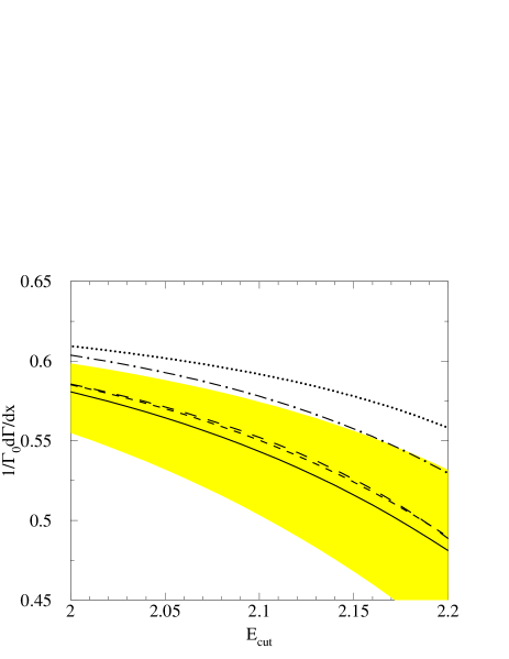
FIG. 3.: The rate integrated from $E_{cut}$. The solid curve is the resummed rate convoluted with the structure function in Eq. (28), using the central values of $(\bar{\Lambda},\ \lambda_{1})$. The shaded region shows the uncertainty due to varying the values of $(\bar{\Lambda},\ \lambda_{1})$ by one sigma. The dotted curve is the one loop rate without the structure function. The long dashed curve is the resummed rate without the structure function. The dot-dashed curve is the one loop rate convoluted with the structure function, using the central values of $(\bar{\Lambda},\ \lambda_{1})$. The short dashed curve is the one loop rate and the $O(\alpha_{s}^{2})$ piece from the resummation, convoluted with the structure function.

In Fig. 3 we show the rate as a function of the lower cut on the photon energy, for the ansatz in Eq. (28) and with the central values for $(\bar{\Lambda},\ \lambda_{1})$. In this plot we also show the rate with and without perturbative resummation without the inclusion of the structure function, and the one loop rate as well as the one loop rate plus the $O(\alpha_{s}^{2})$ piece from the expansion of the resummed rate, convoluted with the structure function. As expected, the effects of both perturbative and non-perturbative resummation are enhanced as the photonic energy cut is increased. We see again that the dominant piece of the resummation is coming from the $O(\alpha_{s}^{2})$ term. Furthermore, the inclusion of the structure function does not significantly enhance the effects of the resummation for these choices of structure functions. If they died off more slowly for large negative $k_{+}$, we would expect the logs to be enhanced. The shaded region is the resummed rate using the one sigma values for $(\bar{\Lambda},\ \lambda_{1})$, with again the structure function defined in Eq. (28). We see that, as $\bar{\Lambda}$ is increased, the effects of resummation become more important, as one would expect since the width of the primordial distribution is increasing. Varying the width $(\bar{\Lambda},\ \lambda_{1})$, is one way of determining the uncertainty due to our ignorance of the structure function. Another method would be varying the functional form of the structure function itself (i.e. changing the higher moments).

FIG. 4.: Rate convoluted with the different structure functions. The solid curve is the rate convoluted with the Eq. (29), and the dashed curve is the rate convoluted with Eq. (29).

In Fig. 4, we compare the rates for the two differing functional forms given by Eq. (28) and Eq. (29). We see that the rate is not as sensitive to the higher moments as it is to the lower moments $(\bar{\Lambda},\ \lambda_{1})$. Note that for these particular choices of the structure function the fourth and fifth moments differ by only $O(50\%)$. So perhaps a more thorough search of the possible form of the structure functions should be explored. Assuming that the structure function is well behaved (read physically motivated), the dominant uncertainty in the rate due to our ignorance of the structure function can be removed once we have a better determination of $(\bar{\Lambda},\ \lambda_{1})$.

Finally, we may investigate the convergence of the expansion of $g_{1}$ in the exponent with the inclusion of the structure function. In Fig. 5 we show the rate for the series expansion of $g_{1}$ up to $O(\alpha_{s}^{3})$, we see that it is indeed well behaved and converges rapidly. This again is signaling that the resummation is not collecting a set of dominant terms.

FIG. 5.: Rate convoluted with the structure function Eq.(28). The dotted curve corresponds to expanding $g_{1}$ to $O(\alpha_{s})$, the dashed curve is for $g_{1}$ expanded to $O(\alpha_{s}^{2})$, and the dot-dashed curve is expanded to $O(\alpha_{s}^{3})$. The solid curve is the rate with the full $g_{1}$.

VII Conclusions

We conclude that resummation is not necessary, and does not increase the accuracy of the prediction, when the photonic cut is near $2.1{\rm\ GeV}$. Therefore, for the purpose of calculating the total rate, it is consistent to convolve the structure function with the $O(\alpha_{s}$) partonic rate. The dominant errors will then come from our ignorance of the structure function and higher order, in $\alpha_{s}$, corrections to the rate, as well as uncertainties in $\Gamma_{0}$ due to the dependence on the $b$ quark mass (i.e. $\bar{\Lambda}$). We estimate that the uncertainties due to the structure function are at the $20\%$ level, though we believe that a more thorough search of the space of structure functions should be performed. If we assume that the size of the $O(\alpha_{s}^{2})$ corrections are typically of the size of the pieces of the two loop result which we pick off from our resummed rate, then the uncertainty coming from these corrections is on the $10\%$ level. On the other hand, if we wish to extract the structure function from the measurement of the spectrum for $b\rightarrow s\gamma$, in order to utilize it in the extraction of $V_{ub}$, the resummation will most probably be necessary.

- [1] A.V. Manohar and M.B. Wise, Heavy Quark Physics, Cambridge University Press, in press.
- [2] R. Akhoury and I.Z. Rothstein, Phys. Rev. D51 (1995) 1125.
- [3] G. Sterman and G.P. Korchemsky, Phys. Lett. B340 (1994) 96.
- [4] A. Ali and C. Greub, Phys. Lett. B361 (1995) 146.
- [5] A. Kagan and M. Neubert, Euro. Lett. 74 (1995) 3372.
- [6] R.D. Dikeman, M. Shifman, and N.G. Uraltsev, Int. J. Mod. Phys. A11 (1996) 571.
- [7] J. Chay, H. Georgi, and B. Grinstein, Phys. Lett. B247 (1990) 399; M. Voloshin and M. Shifman, Sov. J. Nucl. Phys. 41 (1985) 120.
- [8] M. Neubert, Phys. Rev. D49 (1994) 3392.
- [9] I.I. Bigi, M.A. Shifman, N.G. Uraltsev, and A.I. Vainshtein, Int. J. Mod. Phys. A9 (1994) 2467.
- [10] S. Glenn et al., CLEO Collaboration, CLEO CONF 98-17.
- [11] For a review see, G. Sterman, in QCD and Beyond, Proceedings of the Theoretical Advanced Study Institute in Elementary Particle Physics (TASI 95), ed. D.E. Soper (World Scientific, 1996), p. 327, hep-ph/9606312.
- [12] S. Catani, M.L. Mangano, P. Nason, and L. Trentadue, Nucl. Phys. B478 (1996) 273.
- [13] Z. Ligeti, M. Luke, A.V. Manohar, and M.B. Wise, hep-ph/9903305.
- [14] T. Mannel and M. Neubert, Phys. Rev. D50 (1994) 2037.
- [15] M. Gremm, A. Kapustin, Z. Ligeti, and M.B. Wise, Phys. Rev. Lett. 77 (1996) 20.