Phenomenology of $V_{ub}$ from Ratios of Inclusive $B$ Decay Rates

Abstract

We explore the theoretical feasibility of extracting $V_{ub}$ from two ratios built from $B$ meson inclusive partial decays, $R_{1}=\Gamma(b\to u\bar{c}s^{\prime})/3\Gamma(b\to cl\bar{\nu})$ and $R_{2}=[\Gamma(b\to cX)-\Gamma(b\to\bar{c}X)]/\Gamma(b\to c\bar{u}d^{\prime})$. We discuss contributions to these quantities from perturbative and nonperturbative physics, and show that they can be computed with overall uncertainties at the level of 10%.

I Introduction

The accurate measurement of $V_{ub}$ is one of the most challenging theoretical and experimental problems in $B$ physics. Its value is crucial for constraining the Unitarity Triangle and probing the question of whether the CKM framework is adequate for describing flavor physics in the standard model. The present best experimental values for $V_{ub}$, from the inclusive decay $B\to X_{u}l\bar{\nu}$ and the exclusive process $B\to\rho l\bar{\nu}$, are limited by model-dependence and other theoretical errors. New approaches to extracting $V_{ub}$ from inclusive and exclusive semileptonic decays have been proposed and are promising, but have not yet proven to be viable experimentally.

In light of this situation, new methods for probing $V_{ub}$ are still needed. In a recent paper [1], we suggested that it would be useful to attempt to measure the inclusive production of “wrong sign” charm in $B$ decays, that is, to look for evidence for the quark level transition $b\to u\bar{c}s^{\prime}$. In particular, we proposed to study the ratio $R_{1}=\Gamma(b\to u\bar{c}s^{\prime})/3\Gamma(b\to cl\bar{\nu})$, noting that the theoretical expression for this quantity is in a number of respects particularly well under control. (Here $s^{\prime}$ and $d^{\prime}$ are the flavor eigenstates, and we take $m_{s}=m_{d}=0$.) We went on to compute the leading perturbative and nonperturbative corrections to the parton model result for $R_{1}$. The analysis of Ref. [1] also relied implicitly on the use of parton-hadron duality. This assumption is common to all extractions of $V_{ub}$ from inclusive $B$ decays, and while it is not unreasonable to expect it to hold in this case, there is no rigorous proof that it actually does. Perhaps the near equality of the charged and neutral $B$ meson lifetimes provides some empirical evidence that duality is well respected in $B$ decays.

In this paper we will refine the analysis of Ref. [1] in a number of respects. First, we will include complete radiative corrections to $R_{1}$ at next-to-leading order, that is, all terms proportional to $\alpha_{s}(m_{b})$ and $\alpha_{s}^{n+1}\ln^{n}(m_{W}/m_{b})$. Second, we will include a set of “enhanced” two loop terms, often referred to as “BLM” corrections [2], which are proportional to $\alpha_{s}^{2}\beta_{0}$, where $\beta_{0}=11-2n_{f}/3$ is the first coefficient in the QCD beta function. It was pointed out in Ref. [1] that these terms are not likely to be as large in $R_{1}$ as in, for example $\Gamma(B\to X_{c}l\bar{\nu})$, because of the cancellation of the leading renormalon ambiguity. Indeed, our explicit calculation will show that these terms contribute only at the level of ten percent. Third, in Ref. [1], we also included the leading nonperturbative contributions to the inclusive decay, which come from annihilation processes and are proportional to $16\pi^{2}f_{B}^{2}/m_{b}^{2}$. These terms are formally of order $1/m_{b}^{3}$ but are enhanced by the two-body, rather than three-body, phase space of the final state. We found that in charged $B$ decays, these processes can contribute at the order of 5%, while in neutral $B$ decays they turn out to be negligible. We will have little new to say about these corrections, except that we will attempt to combine the uncertainties from these contributions with those from the radiative corrections to obtain an overall picture of the reliability of the theoretical calculation. We will also take the opportunity to include an additional small “hybrid” contribution of order $\alpha_{s}\ln(m_{W}/m_{b})\lambda_{2}/m_{b}^{2}$.

We will also propose that it is useful to consider a second ratio, $R_{2}=[\Gamma(b\to cX)-\Gamma(b\to\bar{c}X)]/\Gamma(b\to c\bar{u}d^{\prime})$. We will see that $R_{2}$ is theoretically clean in a way which is similar to $R_{1}$, and we will extend all aspects of our analysis of $R_{1}$ to include $R_{2}$. The experimental measurement of $R_{2}$ would certainly be challenging, but the challenges would be distinct from those that confront the measurement of $R_{1}$ and this second ratio deserves separate consideration.

Finally, we will close by presenting an overall picture of the theoretical understanding of $R_{1}$ and $R_{2}$, with our best estimate of the remaining uncertainties and the future prospects for reducing them. We hope that this will provide an intriguing goal for our experimental colleagues to aim for.

II $V_{ub}$ from ratios of partial decay rates

In our previous paper [1], we proposed that the quark level process $b\to u\bar{c}s^{\prime}$ would be a promising mode from which to extract $V_{ub}$. Final states with this combination of quark flavors arise only from processes proportional to $V_{ub}$, with no contributions from penguin diagrams or long distance rescattering. In the form of the ratio

$$R_{1}=\Gamma(b\to u\bar{c}s^{\prime})/3\Gamma(b\to cl\bar{\nu})\,,$$ (1)

the theoretical expression is very well behaved. The phase space dependence on $x_{c}=m_{c}^{2}/m_{b}^{2}$ is identical in the numerator and denominator, as are the leading nonperturbative corrections of order $1/m_{b}^{2}$. At tree level and in the limit $m_{b}\to\infty$, then, we have simply

$$R_{1}=|V_{ub}/V_{cb}|^{2}\,\left\{1+O(\alpha_{s},1/m_{b}^{2})\right\}\,.$$ (2)

In Ref. [1], we first included radiative corrections at leading logarithmic order, which has the effect of multiplying the expression for $R_{1}$ by a factor $\chi\simeq 1.09$. We also computed the leading radiative correction to the decay processes $b\to u\bar{c}s^{\prime}$ and $b\to cl\bar{\nu}$, which although formally subleading is numerically substantial. The result was an expression of the form

$$R_{1}=\chi\,|V_{ub}/V_{cb}|^{2}\,\left\{1+g(x_{c}){\alpha_{s}\over\pi}+\ldots\right\}\,.$$ (3)

With $x_{c}=0.09$ and $\alpha_{s}=\alpha_{s}(m_{b})=0.22$, the one loop radiative correction is $g\alpha_{s}/\pi=0.21$, so indeed it is large and should be included. However, the scale $\mu$ at which $\alpha_{s}$ ought to be evaluated was not fixed by our calculation, leading to a significant remaining uncertainty. This can be resolved only with a full next-to-leading order calculation, which we will perform in the next section. We will find that the partial calculation of Ref. [1] was correct to within approximately 20%.

Unfortunately, the experimental measurement of $R_{1}$ is extremely challenging. The largest background to observing the quark level process $b\to u\bar{c}s^{\prime}$ is $b\to c\bar{c}s^{\prime}$, the rate for which is approximately a factor of 100 larger. The measurement is made more difficult by the fact that the only quantity which is well predicted theoretically is the ratio of fully inclusive rates, while many of the experimental techniques for rejecting $b\to c\bar{c}s^{\prime}$ involve tagging on a particular hadronic final state. Although the measurement of $R_{1}$ may be feasible, it will hardly be straightforward. Nevertheless, relevant experimental techniques already are being developed [3], and the excellent capability of the BaBar and BELLE detectors to vertex individually the boosted $B$ mesons also will improve the prospects for this measurement [4].

There is another ratio which one might consider, which avoids the necessity of rejecting the $b\to c\bar{c}s^{\prime}$ background. Let $\Gamma(b\to cX)=\Gamma(b\to c\bar{u}d^{\prime})+\Gamma(b\to c\bar{c}s^{\prime})$ be the fully inclusive production of $c$ in nonleptonic $b$ decays, and $\Gamma(b\to\bar{c}X)=\Gamma(b\to u\bar{c}s^{\prime})+\Gamma(b\to c\bar{c}s^{\prime})$ be the inclusive production of $\bar{c}$. Also, define $\Gamma(b\to cX^{\prime})=\Gamma(b\to c\bar{u}d^{\prime})$, that is, the inclusive production of $c$ without an accompanying $\bar{c}$. Note that $\Gamma(b\to c\bar{c}s^{\prime})<\Gamma(b\to c\bar{u}d^{\prime})$, so the measurement of $\Gamma(b\to cX^{\prime})$ does not require rejecting an overwhelming background. Then let

$$R_{2}={\Gamma(b\to cX)-\Gamma(b\to\bar{c}X)\over\Gamma(b\to cX^{\prime})}\equiv 1-\delta_{2}\,.$$ (4)

We see that $\Gamma(b\to c\bar{c}s^{\prime})$ cancels in the numerator of $R_{2}$. In terms of quark level transitions,

$$\delta_{2}={\Gamma(b\to u\bar{c}s^{\prime})\over\Gamma(b\to c\bar{u}d^{\prime})}\,.$$ (5)

At tree level, $\delta_{2}=|V_{ub}/V_{cb}|^{2}$. Unlike in $R_{1}$, there is no leading logarithmic correction to $\delta_{2}$, since these contribute identically to the numerator and the denominator. The leading radiative correction arises at order $\alpha_{s}(m_{b})$, and the leading nonperturbative corrections at order $\alpha_{s}\ln(m_{W}/m_{b})\lambda_{2}/m_{b}^{2}$ and $16\pi^{2}f_{B}^{2}/m_{b}^{2}$.

The experimental advantage of $R_{2}$ is that the large $b\to c\bar{c}s^{\prime}$ background cancels. The difficulty is that in order for $R_{2}$ to be sensitive to $|V_{ub}/V_{cb}|^{2}$, both $\Gamma(b\to cX)$ and $\Gamma(b\to cX^{\prime})$ must be measured with an accuracy of better than 1%. This may prove to be as challenging as rejecting $b\to c\bar{c}s^{\prime}$, or even more so, but it involves a distinct set of problems. It will be up to the experimental community to determine whether this measurement is feasible or not.

A quantity which would be more attractive experimentally is

$$R_{3}={\Gamma(b\to cX)-\Gamma(b\to\bar{c}X)\over\Gamma(b\to cl\bar{\nu})}\,,$$ (6)

since doing so avoids the requirement of determining $\Gamma(b\to cX^{\prime})$ precisely. Unfortunately, $R_{3}$ cannot be computed with the very small uncertainties of $R_{1}$ and $R_{2}$. This is simply because, unlike $R_{1}$ and $R_{2}$, the calculation of $R_{3}$ requires that the ratio $\Gamma(b\to cX^{\prime})/\Gamma(b\to cl\bar{\nu})=R_{1}/\delta_{2}$ be known with a theoretical accuracy of better than 1%. This is well beyond the level of precision presently attainable, due to the perturbative and nonperturbative contributions which we will discuss below. Thus, we will not consider $R_{3}$ further. However, we do note that in anticipation of theoretical advances, it may well be useful for experimentalists to measure $R_{3}$ as well as $R_{1}$ and $R_{2}$. Alternatively, if $\Gamma(b\to cX^{\prime})/\Gamma(b\to cl\bar{\nu})$ could itself be measured with the required precision, then it could be used to construct $R_{2}$ from the experimentally more accessible ratio $R_{3}$.

III Radiative corrections at next-to-leading order

In Ref. [1], we included two subsets of radiative corrections. First, we used an effective Lagrangian evaluated at the scale $\mu=m_{b}$,

$${\cal L}=-\frac{4G_{F}}{\sqrt{2}}\,V_{ub}\,\Bigl{[}C_{1}(\mu)\bar{u}_{\alpha}\gamma_{\mu}P_{L}b_{\alpha}\,\bar{s}^{\prime}_{\beta}\gamma^{\mu}P_{L}c_{\beta}+C_{2}(\mu)\bar{u}_{\alpha}\gamma_{\mu}P_{L}b_{\beta}\,\bar{s}^{\prime}_{\beta}\gamma^{\mu}P_{L}c_{\alpha}\Bigr{]}+{\rm h.c.}\,.$$ (7)

Employing such a Lagrangian has the effect of summing all logarithms of the form $\alpha_{s}^{n}\ln^{n}(m_{W}/m_{b})$. At leading log order, $C_{1}(m_{b})\simeq 1.11$ and $C_{2}(m_{b})\simeq-0.24$ [5]. Second, we performed a partial one-loop calculation of the radiative correction to the decay rate itself. Although we included the largest contributions, our calculation was incomplete because we omitted terms which were not proportional to $(C_{1}+C_{2}/N_{c})^{2}$. This allowed us to consider only gluon exchanges within color-singlet currents, simplifying the result enormously. At leading log order terms of this form contribute 96% of the total decay rate, so we hoped that the error from this approximation would not be too large. The combined radiative correction which we found, keeping all terms of order $\alpha_{s}^{n}\ln^{n}(m_{W}/m_{b})$ and of order $\alpha_{s}$ but only some of order $\alpha_{s}^{2}\ln(m_{W}/m_{b})$, was $\chi[1+g(x_{c})\alpha_{s}/\pi]$, where $\chi$ came from QCD running between $M_{W}$ and $m_{b}$ and $g(x_{c})$ was a finite radiative correction to the decay rate. For $x_{c}=0.09$ and $\alpha_{s}=\alpha_{s}(m_{b})=0.21$, this gave 1.32, or a combined correction of about 30%.

The largest ambiguity in this result comes from the scale $\mu$ at which the one-loop correction to the decay process is to be evaluated. This ambiguity can be removed only by performing a full calculation at next-to-leading log order, including consistently all terms of order $\alpha_{s}^{n+1}\ln^{n}(m_{W}/m_{b})$. We present the results of such a calculation here. We have followed closely the analogous calculation of $b\to c\bar{u}d^{\prime}$ by Bagan et al. [6], and have used their partial results where appropriate.

We refer the reader to the excellent exposition of Ref. [6] for a detailed discussion of the method of the analysis, and here present only our results. A brief synopsis of our calculation is found in the Appendix. We write the answer in the form

$$R_{1}=|V_{ub}/V_{cb}|^{2}\,\left\{1+r_{1}(\mu,x_{c})+\dots\right\}\,,$$ (8)

$$\delta_{2}=|V_{ub}/V_{cb}|^{2}\,\left\{1+r_{2}(\mu,x_{c})+\dots\right\}\,,$$ (9)

where $r_{i}(\mu,x_{c})$ are of order $\alpha_{s}$. Here $\mu$ is the renormalization scale and $x_{c}=m_{c}^{2}/m_{b}^{2}$ is the ratio of the heavy quark pole masses. We take $m_{q}=0$ for $q=u,d,s$, which is in this process an excellent approximation even for the strange quark.

Taking the reference values $m_{b}=4.80\,$GeV, $m_{c}=1.45\,$GeV (so $x_{c}=0.09$), and $\mu=4.8\,$GeV, we find

$$r_{1}(\mu,x_{c})=0.40\qquad{\rm and}\qquad r_{2}(\mu,x_{c})=0.12\,.$$ (10)

Because the leading logarithms cancel in the ratio $\delta_{2}$, $r_{2}$ starts at order $\alpha_{s}$ rather than at order $\alpha_{s}\ln(M_{W}/m_{b})$ and is considerably smaller than $r_{1}$. In Fig. 1, we display the variation of $r_{i}$ with $x_{c}$ and $\mu$.

     

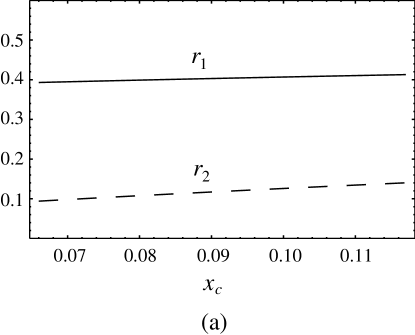
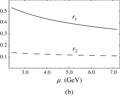
FIG. 1.: Variation of $r_{i}$ with $x_{c}$ and $\mu$. (a) $r_{i}(x_{c})$ for $4.5\,{\rm GeV}\leq m_{b}\leq 5.1\,{\rm GeV}$ and $\mu=m_{b}$. (b) $r_{i}(\mu)$ for $2.4\,{\rm GeV}\leq\mu\leq 7.2\,{\rm GeV}$ and $m_{b}=4.8$ GeV.

In Fig. 1a, we vary $m_{b}$ between $4.5\,$GeV and $5.1\,$GeV, fixing $m_{c}$ by the heavy quark symmetry constraint $m_{b}-m_{c}=3.35\,$GeV and taking $\mu=m_{b}$. We see that the dependence on $x_{c}$ is very mild; over the conservative range considered, $r_{1}$ varies by $\pm 0.01$ and $r_{2}$ by $\pm 0.02$. In Fig. 1b, we fix $m_{b}=4.8\,$GeV and vary $\mu$ between ${1\over 2}m_{b}$ and ${3\over 2}m_{b}$. For $r_{2}$, the dependence is soft, approximately $\pm 0.02$. However, for $r_{1}$ a significant $\mu$-dependence remains even at next-to-leading order. For $\mu$ as low as ${1\over 2}m_{b}$, we have $r_{1}=0.53$. We will choose to assign an asymmetrical error of $(+0.10,-0.05)$ to the $\mu$-dependence of $r_{1}$. Combining the variation in $x_{c}$ and $\mu$, then, we find the results

$$r_{1}=0.40^{+0.10}_{-0.05}\qquad{\rm and}\qquad r_{2}=0.12\pm 0.03\,.$$ (11)

In the partial calculation of our previous paper, we found $\chi(1+g\alpha_{s}/\pi)=1.32$, to be compared with $1+r_{1}$ here. We now see that this approximation underestimated the correct next-to-leading order result by 0.08, or 20%. While our incomplete treatment gave a reasonable result, including the full calculation at this order turns out to be important.

IV BLM Corrections

At the next order in $\alpha_{s}$, a consistent leading-log calculation requires the three-loop anomalous dimensions of the operators in ${\cal L}$ and the two-loop matrix elements. However, since the effects of the running are not large, a useful estimate of these corrections is obtained by simply taking the two-loop matrix element of the singlet operator; this corresponds to neglecting terms of order $\alpha_{s}^{3}\ln(m_{W}/m_{b})$ relative to $\alpha_{s}^{2}$. A further simplification is obtained by only retaining the so-called “BLM” two-loop corrections [2], which are enhanced by a factor of $\beta_{0}\equiv 11-2N_{f}/3$, where $N_{f}=3$ is the number of light quark flavors. This class of two-loop corrections is computed easily by performing a weighted integral over the one-loop result calculated with a gluon mass [7]. While the BLM corrections are not formally dominant in any limit of QCD, in many processes they are found empirically to be the largest part of the two-loop term. In this section we calculate the BLM corrections to $R_{1}$ and $\delta_{2}$.

These ratios require the BLM corrections to $b\rightarrow u\bar{c}s^{\prime}$, $b\rightarrow c\bar{u}d^{\prime}$ and $b\rightarrow cl\bar{\nu}$. The calculation of the BLM corrections to $b\rightarrow u\bar{c}s^{\prime}$ is identical to that for $b\rightarrow c\bar{c}s^{\prime}$ [8] with one of the charm quark masses set to zero, so we refer the reader to Ref. [8] for details. The corrections are particularly simple because the corrections to the $bu$ and $\bar{c}s^{\prime}$ currents factorize. This feature also allows the BLM corrections to $b\rightarrow c\bar{u}d^{\prime}$ to be extracted easily from existing calculations of the semileptonic decay rate and $R(e^{+}e^{-}\rightarrow\mbox{hadrons})$. Finally, the BLM corrections to semileptonic $b\rightarrow c$ decays were calculated in Ref. [9]. Writing each decay rate as

$$\Gamma(b\rightarrow X)\propto 1+a_{1}^{X}\,{\alpha_{s}(m_{b})\over\pi}+a_{2}^{X}\,\beta_{0}\left({\alpha_{s}(m_{b})\over\pi}\right)^{2}+\dots,$$ (12)

we plot the $a_{i}^{X}$’s in Fig. 2 for each of the relevant decays.

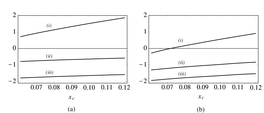
FIG. 2.: (a) The one-loop coefficient $a_{1}^{X}$ and (b) the BLM-enhanced two-loop coefficient $a_{2}^{X}$ to (i) $b\rightarrow u\bar{c}s$, (ii) $b\rightarrow c\bar{u}d$ and (iii) $b\rightarrow cl\bar{\nu}$ decays.

For the purpose of evaluating the quality of the perturbation series for the matrix elements, one should compare this two loop result to the one loop correction $g(x_{c})$ defined in Eq. (3). The reason is that neither the BLM correction nor $g(x_{c})$ has a logarithmic dependence on $M_{W}$. Hence we neglect for the moment the full NLO corrections of the previous section and write

$$R_{1}=\chi\left|{V_{ub}\over V_{cb}}\right|^{2}\left\{1+g_{1}(x_{c}){\alpha_{s}(m_{b})\over\pi}+f_{1}(x_{c})\beta_{0}\left({\alpha_{s}(m_{b})\over\pi}\right)^{2}+\dots\right\}\,,$$ (13)

$$\delta_{2}=\left|{V_{ub}\over V_{cb}}\right|^{2}\left\{1+g_{2}(x_{c}){\alpha_{s}(m_{b})\over\pi}+f_{2}(x_{c})\beta_{0}\left({\alpha_{s}(m_{b})\over\pi}\right)^{2}+\dots\right\}\,.$$ (14)

The coefficients $g_{i}(x_{c})$ and $f_{i}(x_{c})$ are plotted in Fig. 3.

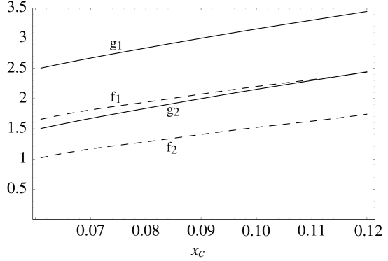
FIG. 3.: The one-loop coefficients $g_{i}$ (solid) and BLM-enhanced two-loop coefficients $f_{i}$ (dashed).

Taking $x_{c}=0.09$ and $\mu=m_{b}$, we find for $R_{1}$ the results

$$g_{1}(0.09)\,{\alpha_{s}(m_{b})\over\pi}=3.0\,{\alpha_{s}(m_{b})\over\pi}=0.21\,,$$ (15)

$$f_{1}(0.09)\,\beta_{0}\left({\alpha_{s}(m_{b})\over\pi}\right)^{2}=2.1\,\beta_{0}\left({\alpha_{s}(m_{b})\over\pi}\right)^{2}=0.09\,,$$ (16)

and for $\delta_{2}$,

$$g_{2}(0.09)\,{\alpha_{s}(m_{b})\over\pi}=2.0\,{\alpha_{s}(m_{b})\over\pi}=0.14\,,$$ (17)

$$f_{2}(0.09)\,\beta_{0}\left({\alpha_{s}(m_{b})\over\pi}\right)^{2}=1.4\,\beta_{0}\left({\alpha_{s}(m_{b})\over\pi}\right)^{2}=0.06\,.$$ (18)

While it is not formally consistent to include these corrections in the NLO calculations of the previous section, we can use them to shift the central values of the $r_{i}$’s,

$$r_{1}(\mu=m_{b},x_{c}=0.09) \rightarrow r_{1}+1.09\times f_{1}(0.09)=0.40+0.10=0.50\,,$$ (19)

$$r_{2}(\mu=m_{b},x_{c}=0.09) \rightarrow r_{2}+f_{2}(0.09)=0.12+0.06=0.18\,.$$ (20)

Note that both corrections are somewhat larger than the error estimates from varying the renormalization scale in the previous section. Varying $m_{b}$ between 4.5 GeV and 5.1 GeV yields an additional uncertainty, which we estimate to be $(+0.005,-0.025)$ on $r_{1}$ and $\pm 0.015$ on $r_{2}$.

V Nonperturbative corrections

In addition to the perturbative corrections discussed so far, there are also nonperturbative contributions to $R_{1}$ and $\delta_{2}$ which are sensitive to the configuration of the initial $B$ meson. As discussed in Ref. [1], the cancellation of the tree level phase space factor eliminates terms in $R_{1}$ of order $\Lambda_{\rm QCD}/m_{b}$. Furthermore, while there could be in principle subleading terms at order $1/m_{b}^{2}$ proportional to the HQET parameters $\lambda_{1}$ and $\lambda_{2}$ [10], these cancel in the ratio as well.

This can be understood by examining the possible sources of dependence on the charm quark mass. These corrections enter the calculations of $b\to u\bar{c}s^{\prime}$ and $b\to c\bar{u}d^{\prime}$ either from kinematic phase space functions or from performing spin sums. Consider the Fierzed form of the effective Lagrangian (7),

$${\cal L}=-\frac{4G_{F}}{\sqrt{2}}\,V_{ub}\,\Bigl{[}C_{1}(\mu)\bar{s}^{\prime}_{\beta}\gamma_{\mu}P_{L}b_{\alpha}\,\bar{u}_{\alpha}\gamma^{\mu}P_{L}c_{\beta}+C_{2}(\mu)\bar{s}^{\prime}_{\beta}\gamma_{\mu}P_{L}b_{\beta}\,\bar{s}^{\prime}_{\beta}\bar{u}_{\alpha}\gamma^{\mu}P_{L}c_{\alpha}\Bigr{]}+{\rm h.c.}\,.$$ (21)

Substituting $s^{\prime}\to d^{\prime}$ and $V_{ub}\to V_{cb}$, and exchanging $u$ and $c$, we obtain the Lagrangian responsible for $b\to c\bar{u}d^{\prime}$. Recall that we take $m_{d}=m_{s}=0$. The calculation of the decay $b\to c\bar{u}d^{\prime}$ involves the computation of the polarization tensor with a massive $c$ quark and a massless $\bar{u}$ antiquark, whereas the $b\to u\bar{c}s^{\prime}$ decay involves a massless $u$ and a massive $\bar{c}$. Hence the Fierz transformation by itself does not guarantee the cancellation of all terms in the ratios $R_{i}$. However, because of the $VV-AA$ structure of the polarization tensor, and the fact that $VV$ and $AA$ correlation functions are symmetric under $m_{u}\leftrightarrow m_{c}$ [11], the total decay rate is also symmetric under interchange of the quark masses. Thus, both the phase space and $1/m_{b}^{2}$ corrections cancel in $\delta_{2}$. To extend the argument to $R_{1}$, note that in the Fierzed form and at tree level, the decay $b\to c\bar{u}d^{\prime}$ is the same as $b\to u\tau\bar{\nu}_{\tau}$, for which the nonperturbative corrections were computed in Ref. [12]. This discussion elaborates the observation made in Ref. [1] that these corrections cancel. A general argument that the terms proportional to $\lambda_{1}$ (but not to $\lambda_{2}$) cancel in all ratios of $B$ decays was given in Ref. [13].

There remain, however, mixed terms proportional to $\alpha_{s}\lambda_{2}/m_{b}^{2}$, which need not cancel in the ratios. Recall that $\lambda_{2}=\langle B|\,\bar{b}_{v}g\sigma\cdot Gb_{v}\,|B\rangle/12M_{B}$, where $b_{v}$ is the effective $b$ field of HQET, is related to the hyperfine interaction of the $b$ quark chromomagnetic moment with the light degrees of freedom in the $B$ meson [10, 13]. The chromomagnetic operator is obtained by attaching a gluon to one of the quarks in the final state, before the operator product expansion is performed. In the effective theory defined by the Lagrangian (7), terms of order $\alpha_{s}\lambda_{2}$ come from two sources. First, they arise from one-loop radiative corrections to the operator product expansion itself, in which case they are quite small. Second, the color structure allows terms proportional to $C_{1}C_{2}$ to arise at tree level from the interference of the color singlet and color exchanged operators. These terms are really of order $\alpha_{s}\ln(M_{W}/m_{b})\lambda_{2}/m_{b}^{2}$ and hence are enhanced over the others. They were first calculated for the decay $b\to c\bar{u}d^{\prime}$ in Ref. [13].

In fact, a straightforward argument shows that these terms are equal in size and of the opposite sign in $b\to u\bar{c}s^{\prime}$ as compared to $b\to c\bar{u}d^{\prime}$. Consider again the Fierzed form of the effective Lagrangian (21). Because of the color structure when the operators are written in this form, the term proportional to $C_{1}C_{2}\lambda_{2}$ is generated by attaching a gluon to the $\bar{c}u$ loop, performing the operator product expansion, and extracting the chromomagnetic moment operator $\bar{b}\sigma^{\mu\nu}G_{\mu\nu}b$. This term is odd under the exchange $u\to c$ and $\bar{c}\to\bar{u}$, or equivalently $m_{u}^{2}\leftrightarrow m_{c}^{2}$, which can be seen immediately by inspection of the relevant Feynman diagrams. Alternatively, simply note that the quark and antiquark produced by the left-handed current carry opposite magnetic moments. To obtain the result for $b\to u\bar{c}s^{\prime}$, we take the limit $m_{u}=0$; as noted above, for $b\to c\bar{u}d^{\prime}$, we can take $m_{c}=0$ and $m_{u}\to m_{c}$. Since the general result is odd in $(m_{c}^{2}-m_{u}^{2})$, the two limiting results are the negatives of each other, as promised.

We write the result as fractional corrections to $R_{1}$ and $\delta_{2}$ (suppressing for the moment the radiative corrections of the previous sections),

$$R_{1} = |V_{ub}/V_{cb}|^{2}\,\Big{\{}1+\ell_{2}(\mu,x_{c})+\dots\Big{\}}\,,$$ (22)

$$\delta_{2} = |V_{ub}/V_{cb}|^{2}\,\Big{\{}1+2\ell_{2}(\mu,x_{c})+\dots\Big{\}}\,,$$ (23)

where

$$\ell_{2}(\mu,x_{c})=C_{1}(\mu)C_{2}(\mu)\,{16(1-x_{c})^{3}\over f(x_{c})}\,{\lambda_{2}(\mu)\over m_{b}^{2}}$$ (24)

and $f(x_{c})=1-8x_{c}+8x_{c}^{3}-x_{c}^{4}-12x_{c}^{2}\ln x_{c}$ is the tree level phase space function. For consistency, $C_{1}(\mu)$ and $C_{2}(\mu)$ should be evaluated at leading order, to include only terms of order $\alpha_{s}^{n}\ln^{n}(M_{W}/m_{b})\lambda_{2}/m_{b}^{2}$. The scale dependence of $\lambda_{2}$ is given by [14]

$$\lambda_{2}(\mu)=\lambda_{2}(m_{b})\Big{[}\alpha_{s}(\mu)/\alpha_{s}(m_{b})\Big{]}^{9/25}\,.$$ (25)

For $\mu=m_{b}=4.8\,$GeV, and with $\lambda_{2}(m_{b})=0.12\,$GeV fixed by the $B-B^{*}$ mass splitting [14], we find $\ell_{2}=-0.036$. The variation of $\ell_{2}$ with $x_{c}$ and $\mu$ is shown in Fig. 4.

     

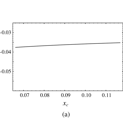
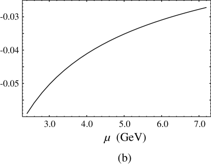
FIG. 4.: Variation of $\ell_{2}$ with $x_{c}$ and $\mu$. (a) $\ell_{2}(x_{c})$ for $4.5\,{\rm GeV}\leq m_{b}\leq 5.1\,{\rm GeV}$ and $\mu=m_{b}$. (b) $\ell_{2}(\mu)$ for $2.4\,{\rm GeV}\leq\mu\leq 7.2\,{\rm GeV}$ and $m_{b}=4.8$ GeV.

We see that, as with the radiative corrections, the only significant uncertainty comes from the choice of renormalization scale. We assign the tiny error $\pm 0.001$ to $\ell_{2}$ from the variation with $x_{c}$, and the larger asymmetrical error $(+0.010,-0.015)$ to the variation with $\mu$. Combining these in quadrature, we see that the first is negligible, and we estimate

$$\ell_{2}=-0.036^{+0.010}_{-0.015}\,.$$ (26)

Noting that the fractional correction to $\delta_{2}$ is $2\ell_{2}$ and comparing to the radiative correction $r_{2}$ (11), we see that this is actually an important uncertainty for $\delta_{2}$.

The leading purely nonperturbative corrections to $R_{1}$ and $\delta_{2}$ arise at order $1/m_{b}^{3}$. The largest such corrections are associated with annihilation processes such as $b\bar{u}\to\bar{c}s^{\prime}$, since they are enhanced by a relative phase space factor of $16\pi^{2}$. They are also spectator dependent, contributing differently to $B^{-}$ and $\overline{B}{}^{0}$ decays. In Ref. [1], we discussed the derivation and computed the annihilation terms in $R_{1}$. Here we will recall those results, as well as present results for $\delta_{2}$. As before, we will present a fractional correction, of the form

$$R_{1} = |V_{ub}/V_{cb}|^{2}\,\Big{\{}1+a_{1}(B^{-},\overline{B}{}^{0})+\dots\Big{\}}\,,$$ (27)

$$\delta_{2} = |V_{ub}/V_{cb}|^{2}\,\Big{\{}1+a_{2}(B^{-},\overline{B}{}^{0})+\dots\Big{\}}\,,$$ (28)

where all other corrections have been momentarily suppressed. The terms $a_{i}$ depend on nonperturbative matrix elements of four-quark operators, parameterized by “bag factors” $B_{i}$ and $\epsilon_{i}$ [15]:

$$\langle B_{q}|\,\bar{b}_{L}\gamma^{\mu}q_{L}\,\bar{q}_{L}\gamma_{\mu}b_{L}\,|B_{q}\rangle = \textstyle{1\over 4}\,f_{B_{q}}^{2}m_{B_{q}}^{2}\,B_{1}\,,$$ (29)

$$\langle B_{q}|\,\bar{b}_{R}q_{L}\,\bar{q}_{L}b_{R}\,|B_{q}\rangle = \textstyle{1\over 4}\,f_{B_{q}}^{2}m_{B_{q}}^{2}\,B_{2}\,,$$ (30)

$$\langle B_{q}|\,\bar{b}_{L}\gamma^{\mu}T^{a}q_{L}\,\bar{q}_{L}\gamma_{\mu}T^{a}b_{L}\,|B_{q}\rangle = \textstyle{1\over 4}\,f_{B_{q}}^{2}m_{B_{q}}^{2}\,\epsilon_{1}\,,$$ (31)

$$\langle B_{q}|\,\bar{b}_{R}T^{a}q_{L}\,\bar{q}_{L}T^{a}b_{R}\,|B_{q}\rangle = \textstyle{1\over 4}\,f_{B_{q}}^{2}m_{B_{q}}^{2}\,\epsilon_{2}\,.$$ (32)

In the vacuum insertion ansatz, only color single operators contribute to the decay and we have $B_{1}=B_{2}=1$ and $\epsilon_{1}=\epsilon_{2}=0$. More generally, the color octet parameters $\epsilon_{i}$ are of order $1/N_{c}$ in the limit $N_{c}\to\infty$.

In terms of these parameters, we find the corrections

$$a_{1}(B^{-}) = {16\pi^{2}f_{B}^{2}(1-x_{c})^{2}\over m_{b}^{2}f(x_{c})}\,\Big{\{}(C_{1}+\textstyle{1\over 3}C_{2})^{2}\big{[}(1+2x_{c})B_{2}-(1+\textstyle{1\over 2}x_{c})B_{1}\big{]}$$ (34)

$$\qquad\qquad\qquad\qquad\mbox{}+\textstyle{2\over 3}C_{2}^{2}\big{[}(1+2x_{c})\epsilon_{2}-(1+\textstyle{1\over 2}x_{c})\epsilon_{1}\big{]}\Big{\}}\,,$$

$$a_{1}(\overline{B}{}^{0}) = {16\pi^{2}f_{B}^{2}(1-x_{c})^{2}\over m_{b}^{2}f(x_{c})}\,\sin^{2}\theta_{C}\,\Big{\{}(C_{2}+\textstyle{1\over 3}C_{1})^{2}\big{[}(1+2x_{c})B_{2}-(1+\textstyle{1\over 2}x_{c})B_{1}\big{]}$$ (36)

$$\qquad\qquad\qquad\qquad\mbox{}+\textstyle{2\over 3}C_{1}^{2}\big{[}(1+2x_{c})\epsilon_{2}-(1+\textstyle{1\over 2}x_{c})\epsilon_{1}\big{]}\Big{\}}$$

for $R_{1}$, and

$$a_{2}(B^{-}) = {16\pi^{2}f_{B}^{2}(1-x_{c})^{2}\over m_{b}^{2}f(x_{c})}\,\Big{\{}(C_{1}+\textstyle{1\over 3}C_{2})^{2}\big{[}(1+2x_{c})B_{2}-(1+\textstyle{1\over 2}x_{c})B_{1}\big{]}$$ (39)

$$\qquad\qquad\qquad\qquad\mbox{}+\textstyle{2\over 3}C_{2}^{2}\big{[}(1+2x_{c})\epsilon_{2}-(1+\textstyle{1\over 2}x_{c})\epsilon_{1}\big{]}$$

$$\qquad\qquad\qquad\qquad-\textstyle{1\over 3}(C_{1}^{2}+6C_{1}C_{2}+C_{2}^{2})B_{1}-2(C_{1}^{2}+C_{2}^{2})\epsilon_{1}\Big{\}}\,,$$

$$a_{2}(\overline{B}{}^{0}) = -{16\pi^{2}f_{B}^{2}(1-x_{c})^{2}\over m_{b}^{2}f(x_{c})}\,\cos 2\theta_{C}\,\Big{\{}(C_{2}+\textstyle{1\over 3}C_{1})^{2}\big{[}(1+2x_{c})B_{2}-(1+\textstyle{1\over 2}x_{c})B_{1}\big{]}$$ (41)

$$\qquad\qquad\qquad\qquad\qquad\qquad\mbox{}+\textstyle{2\over 3}C_{1}^{2}\big{[}(1+2x_{c})\epsilon_{2}-(1+\textstyle{1\over 2}x_{c})\epsilon_{1}\big{]}\Big{\}}$$

for $\delta_{2}$. In deriving the corrections to the denominator of $\delta_{2}$, we have adapted the results of Ref. [15] for the channel $b\to c\bar{u}d^{\prime}$. With $m_{b}=\mu=4.8\,$GeV, $f_{B}=200\,$MeV and $\sin\theta_{C}=0.22$, we find

$$a_{1}(B^{-}) = -0.48B_{1}+0.54B_{2}-0.018\epsilon_{1}+0.021\epsilon_{2}\,,$$ (42)

$$a_{1}(\overline{B}{}^{0}) = -0.00034B_{1}+0.00038B_{2}-0.018\epsilon_{1}+0.020\epsilon_{2}\,,$$ (43)

$$a_{2}(B^{-}) = -0.43B_{1}+0.54B_{2}-1.14\epsilon_{1}+0.021\epsilon_{2}\,,$$ (44)

$$a_{2}(\overline{B}{}^{0}) = 0.0063B_{1}-0.0071B_{2}+0.34\epsilon_{1}-0.38\epsilon_{2}\,.$$ (45)

Note that in $a_{2}(B^{-},\overline{B}{}^{0})$, the coefficients of $\epsilon_{i}$ are quite large. This reflects the potentially significant contribution of color-octet annihilation processes to nonleptonic $B$ decays, as observed in Ref. [15]. Since the parameters $\epsilon_{i}$ are not known well, the large size of these terms introduces a problematic uncertainty into the denominator of $\delta_{2}$. If we take the vacuum insertion ansatz, in which $\epsilon_{i}$ do not contribute, we have

$$a_{1}(B^{-}) = 0.062\,,\qquad\qquad a_{1}(\overline{B}{}^{0})=4.4\times 10^{-5}\,,$$ (46)

$$a_{2}(B^{-}) = 0.112\,,\qquad\qquad a_{2}(\overline{B}{}^{0})=-8.1\times 10^{-4}\,.$$ (47)

Unfortunately, it is hard to assess the uncertainty due to nonzero $\epsilon_{i}$. For want of a better procedure, let us survey briefly the available models for estimating the matrix elements (29). The most reliable of these, in principle, is the lattice QCD result [16]

$$B_{1}(m_{b}) = 1.06\pm 0.08\,,\qquad\qquad\ \epsilon_{1}(m_{b})=-0.01\pm 0.03\,,$$ (48)

$$B_{2}(m_{b}) = 1.01\pm 0.06\,,\qquad\qquad\ \epsilon_{2}(m_{b})=-0.02\pm 0.02\,,$$ (49)

where the quoted errors include neither quenching errors nor the systematic uncertainty due to the extrapolation to the chiral limit. Both of these issues can be addressed in future, more precise calculations. There also exist calculations in the framework of QCD sum rules, which give [17]

$$B_{1}\simeq 1\,,\qquad\qquad\epsilon_{1}\simeq-0.15\,,$$ (50)

$$B_{2}\simeq 1\,,\qquad\qquad\epsilon_{2}\simeq 0\,,$$ (51)

and [18]

$$B_{1}(m_{b}) = 1.01\pm 0.01\,,\qquad\qquad\ \epsilon_{1}(m_{b})=-0.08\pm 0.02\,,$$ (52)

$$B_{2}(m_{b}) = 0.99\pm 0.01\,,\qquad\qquad\ \epsilon_{2}(m_{b})=-0.01\pm 0.03\,,$$ (53)

as well as an HQET QCD sum rule calculation which yields [19]

$$B_{1}(m_{b}) = 0.96\pm 0.04\,,\qquad\qquad\ \epsilon_{1}(m_{b})=-0.14\pm 0.01\,,$$ (54)

$$B_{2}(m_{b}) = 0.95\pm 0.02\,,\qquad\qquad\ \epsilon_{2}(m_{b})=-0.08\pm 0.01\,.$$ (55)

While the $B_{i}$’s are consistently within 5% or so of unity, there is a large spread in the values of the $\epsilon_{i}$ parameters. Of course, it makes no sense to “average over models” as a method for assigning values to $B_{i}$ and $\epsilon_{i}$. Instead, we adopt the procedure of taking the lattice QCD results as central values but inflating the errors both to be conservative and to reflect the variety of values which QCD sum rules yield for $\epsilon_{i}$. To be even more conservative, we inflate the errors symmetrically, so that we use the sum rules results to set the magnitude, but not the sign, of the uncertainty in the lattice calculations. The central values and errors which we choose are then

$$B_{1}(m_{b}) = 1.06\pm 0.10\,,\qquad\qquad\ \epsilon_{1}(m_{b})=-0.01\pm 0.10\,,$$ (56)

$$B_{2}(m_{b}) = 1.01\pm 0.10\,,\qquad\qquad\ \epsilon_{2}(m_{b})=-0.02\pm 0.10\,,$$ (57)

One could imagine a less conservative procedure, especially if one had particular confidence in one of the calculations quoted above, but this is not the approach which we will follow.

Inserting these parameters (56) into the solution (42) for the nonperturbative corrections, we find

$$a_{1}(B^{-}) = 0.04\pm 0.07\,,\qquad\qquad a_{1}(\overline{B}{}^{0})=0\pm 0.003\,,$$ (58)

$$a_{2}(B^{-}) = 0.10\pm 0.13\,,\qquad\qquad a_{2}(\overline{B}{}^{0})=0\pm 0.05\,.$$ (59)

Note that the fractional error associated with the weak annihilation contribution is particularly large for $\delta_{2}$ in charged $B$ decays, due to its enhanced sensitivity to $\epsilon_{i}$.

VI Phenomenology of $V_{ub}$ from $R_{1}$ and $R_{2}$

Combining the results of the previous sections, we now present estimates for central values and uncertainties for $R_{1}$ and $\delta_{2}=1-R_{2}$. Due to the sizable flavor-dependent corrections associated with the spectator contributions, we present our results separately for charged and neutral $B$ decays, which we denote by introducing a suitable superscript. Our results take the form

$$R_{1}^{-} = \left|V_{ub}/V_{cb}\right|^{2}\left[1+r_{1}(x_{c},\mu)+{\ell}_{2}(x_{c},\mu)+a_{1}(B^{-})\right],$$ (60)

$$R_{1}^{0} = \left|V_{ub}/V_{cb}\right|^{2}\left[1+r_{1}(x_{c},\mu)+{\ell}_{2}(x_{c},\mu)+a_{1}(\overline{B}{}^{0})\right],$$ (61)

$$\delta_{2}^{-} = \left|V_{ub}/V_{cb}\right|^{2}\left[1+r_{2}(x_{c},\mu)+2{\ell}_{2}(x_{c},\mu)+a_{2}(B^{-})\right],$$ (62)

$$\delta_{2}^{0} = \left|V_{ub}/V_{cb}\right|^{2}\left[1+r_{2}(x_{c},\mu)+2{\ell}_{2}(x_{c},\mu)+a_{2}(\overline{B}{}^{0})\right],$$ (63)

where $r_{i}$ comes from perturbative QCD radiative corrections and $\ell_{2}$ and $a_{i}$ represent fractional corrections due to nonperturbative effects. Putting our results together, we find

$$R_{1}^{-} = \left|V_{ub}/V_{cb}\right|^{2}\left[1.50^{+0.10}_{-0.05}{}^{+0.005}_{-0.025}{}^{+0.010}_{-0.015}\pm 0.07\right],$$ (64)

$$R_{1}^{0} = \left|V_{ub}/V_{cb}\right|^{2}\left[1.46^{+0.10}_{-0.05}{}^{+0.005}_{-0.025}{}^{+0.010}_{-0.015}\pm 0.005\right],$$ (65)

$$\delta_{2}^{-} = \left|V_{ub}/V_{cb}\right|^{2}\left[1.21\pm 0.03\pm 0.015{}^{+0.015}_{-0.030}\pm 0.13\right],$$ (66)

$$\delta_{2}^{0} = \left|V_{ub}/V_{cb}\right|^{2}\left[1.11\pm 0.03\pm 0.015{}^{+0.015}_{-0.030}\pm 0.05\right].$$ (67)

In these expressions, the first error is our estimate of the uncertainty from NLO perturbative QCD corrections, second is due to uncertainty in the BLM part of the two-loop corrections, the third represents uncertainty in the $\alpha_{s}\ln(M_{W}/m_{b})\lambda_{2}/m_{b}^{2}$ term, and fourth is due to spectator-dependent $1/m_{b}^{3}$ effects. We expect the net effect of other $1/m_{b}^{3}$ effects, not enhanced by the phase space factor of $16\pi^{2}$, to be safely below the level of the estimated uncertainty.

We can combine the errors quoted in Eq. (64) by taking into account the correlations among the various sources of theoretical uncertainty. However, we would like to emphasize that this procedure of estimating and combining theoretical errors, while widespread, is purely conventional and has no rigorous statistical meaning. With this in mind, our best estimate of the central values and overall uncertainties is

$$R_{1}^{-}=\left|V_{ub}/V_{cb}\right|^{2}\Big{[}1.50\pm 0.15\Big{]}\,,\qquad\qquad\delta_{2}^{-}=\left|V_{ub}/V_{cb}\right|^{2}\Big{[}1.21\pm 0.15\Big{]}\,,$$ (68)

$$R_{1}^{0}=\left|V_{ub}/V_{cb}\right|^{2}\Big{[}1.46\pm 0.10\Big{]}\,,\qquad\qquad\,\delta_{2}^{0}=\left|V_{ub}/V_{cb}\right|^{2}\Big{[}1.11\pm 0.10\Big{]}\,.$$ (69)

Although the uncertainties are generally smaller for the neutral $B$ decays, in all cases the theoretical errors are at approximately the level of ten percent. For $R_{1}$, the error is dominated by residual uncertainties in the next-to-leading order radiative corrections. Reducing them substantially would require no less than a next-to-next-to-leading order calculation. For $\delta_{2}$, the uncertainties come primarily from the poorly known strong matrix elements needed for the annihilation contributions, especially from the color octet bag factors $\epsilon_{i}$. The best prospect for improvement here is in a future generation of unquenched lattice calculations. Were these to become available, overall theoretical errors in $\delta_{2}$ at the five percent level would be within reach.

In summary, we have studied the possibility of extracting the CKM matrix element $V_{ub}$ from ratios of inclusive nonleptonic $B$ decays. We have shown that the ratios of inclusive decay widths defined by Eqs. (1) and (4) are impressively “clean” theoretically. We have estimated the impact and uncertainty associated with the NLO radiative corrections, and have included the BLM part of the two-loop term. In addition, we have studied the impact of the leading non-perturbative corrections on $R_{1}$ and $R_{2}$. There is no doubt that the measurement of the $R_{1}$ and $R_{2}$ would be a challenging enterprise. Unfortunately, the somewhat experimentally easier ratio of $R_{3}$ of Eq. (6) has larger theoretical uncertainties, from radiative corrections which would need to be computed at better than the 1% level before the method could be used to extract $V_{ub}$. Nonetheless, the ratios $R_{1}$ and $R_{2}$ of nonleptonic decay widths offer a new and tantalizing approach to measuring the important but poorly known CKM matrix element $V_{ub}$.

A

Here we outline the procedure for calculating radiative corrections to $R_{1}$ and $\delta_{2}$ with next-to-leading log (NLO) accuracy. This calculation amounts to the computation of perturbative corrections to $b\to u\bar{c}s^{\prime}$. We follow closely the procedure outlined in Ref. [6].

FIG. 5.: Feynman diagrams for the calculation of QCD corrections to $b\to u\bar{c}s^{\prime}$. Black dots represent insertions of the operator $O_{1}$ or $O_{2}$. Dashed lines represent gluons.

A full NLO calculation of QCD radiative corrections to $b\to u\bar{c}s^{\prime}$ involves the computation of the eleven loop diagrams depicted in Fig. 5. These diagrams can be conveniently “packaged” into five classes. In fact, only the diagrams of a single class will have to be computed, as the others may be extracted from existing calculations of perturbative QCD corrections to polarization tensors and inclusive semileptonic $b$ decays. As discussed in Ref. [6], this is achieved by the application of Fierz relations to $O_{1}=\bar{u}_{\alpha}\gamma_{\mu}P_{L}b_{\alpha}\,\bar{s}^{\prime}_{\beta}\gamma^{\mu}P_{L}c_{\beta}$ and $O_{2}=\bar{u}_{\alpha}\gamma_{\mu}P_{L}b_{\beta}\,\bar{s}^{\prime}_{\beta}\gamma^{\mu}P_{L}c_{\alpha}$ (note that our choice of $O_{1}$ and $O_{2}$ is opposite to that of Ref. [6]). Although in general Fierz symmetry is broken by regularization, Naïve Dimensional Regularization (NDR) along with the choice of evanescent operators advocated in Ref. [20] actually preserves Fierz relations for renormalized operators. This allows us to use the Fierz transformation on a diagram by diagram basis [6], which significantly simplifies the task of computing the graphs of Fig. 5 in the limit of massless $u$ and $s$ quarks.

We use the effective Lagrangian of Eq. (7) calculated at NLO accuracy. It is convenient to define the Wilson coefficients $C_{\pm}(\mu)$ of the multiplicatively renormalized operators $O_{\pm}={1\over 2}(O_{1}\pm O_{2})$. At this order, they are given by

$$C_{\pm}(\mu)=C_{1}(\mu)\pm C_{2}(\mu) = L_{\pm}(\mu)\left[1+\frac{\alpha_{s}(m_{W})-\alpha_{s}(\mu)}{4\pi}\,\frac{\gamma^{(0)}_{\pm}}{2\beta_{0}}\left(\frac{\gamma^{(1)}_{\pm}}{\gamma^{(0)}_{\pm}}-\frac{\beta_{1}}{\beta_{0}}\right)+\frac{\alpha_{s}(m_{W})}{4\pi}\,B_{\pm}\right]$$ (A1)

$$= L_{\pm}(\mu)\left[1+\frac{\alpha_{s}(m_{W})-\alpha_{s}(\mu)}{4\pi}\,R_{\pm}+\frac{\alpha_{s}(\mu)}{4\pi}\,B_{\pm}\right],$$ (A2)

where for $N_{f}$ flavors and $N_{c}=3$ colors the anomalous dimensions $\gamma_{\pm}=\gamma^{(0)}_{\pm}(\alpha_{s}/4\pi)+\gamma^{(1)}_{\pm}(\alpha_{s}/4\pi)^{2}+~{}...$ are $\gamma^{(0)}_{+}=4$, $\gamma^{(0)}_{-}=-8$, $\gamma^{(1)}_{+}=-7+4N_{f}/9$, and $\gamma^{(1)}_{-}=-14-8N_{f}/9$. The QCD $\beta$ function is given by

$$\beta = -g_{s}\left[\beta_{0}\frac{\alpha_{s}}{4\pi}+\beta_{1}\left(\frac{\alpha_{s}}{4\pi}\right)^{2}+\dots\,\right],$$ (A3)

$$\beta_{0} = 11-\frac{2}{3}N_{f}\,,\qquad\beta_{1}=102-\frac{38}{3}N_{f}\,.$$ (A4)

The coefficients of $O_{\pm}$ at leading logarithmic order are

$$L_{\pm}(\mu)=\left(\frac{\alpha_{s}(m_{W})}{\alpha_{s}(\mu)}\right)^{{\gamma^{(0)}_{\pm}}/{2\beta_{0}}}.$$ (A5)

Finally, the result of two loop matching at $\mu=m_{W}$ for the effective Lagrangian (in NDR) is contained in

$$B_{\pm}=\pm B\,\frac{N_{c}\mp 1}{2N_{c}}\,,\qquad{\rm where}\qquad B=11.$$ (A6)

As advocated in Ref. [6], it is useful to combine Eq. (A6) with the anomalous dimensions,

$$R_{\pm}=B_{\pm}+\frac{\gamma^{(0)}_{\pm}}{2\beta_{0}}\left(\frac{\gamma^{(1)}_{\pm}}{\gamma^{(0)}_{\pm}}-\frac{\beta_{1}}{\beta_{0}}\right),$$ (A7)

so that $R_{\pm}$ are independent of the renormalization scheme. Following Ref. [6], the decay rate for $b\to u\bar{c}s^{\prime}$ can be expressed as

$$\Gamma(b\to u\bar{c}s^{\prime}) = {G_{F}^{2}m_{b}^{5}|V_{ub}|^{2}\over 192\pi^{3}}~{}\Biggl{\{}2L_{+}^{2}(\mu)+L_{-}^{2}(\mu)+\frac{\alpha_{s}(m_{W})-\alpha_{s}(\mu)}{\pi}\left[2L_{+}^{2}(\mu)R_{+}+L_{-}^{2}(\mu)R_{-}\right]$$ (A10)

$$\qquad\quad\mbox{}+\frac{\alpha_{s}(\mu)}{2\pi}\left[\left[L_{+}(\mu)+L_{-}(\mu)\right]^{2}c_{22}(x_{c})+\left[L_{+}(\mu)-L_{-}(\mu)\right]^{2}c_{11}(x_{c})\right]$$

$$\qquad\quad\mbox{}+\frac{\alpha_{s}(\mu)}{3\pi}\left[L_{+}(\mu)^{2}-L_{-}^{2}(\mu)\right]c_{12}(x_{c})\Biggr{\}}\,,$$

where we define $c_{11}(x_{c})=G_{c}+G_{d}$, $c_{22}(x_{c})=G_{a}+G_{b}$, and $c_{12}(x_{c})=G_{a}+G_{b}+G_{e}+B$. Here the five classes of graphs $G_{i}$ are defined as

$$\frac{\alpha_{s}}{\pi}G_{a} = K~{}Im\Big{[}(2)+(2)^{\dagger}+(3)+(9)+(9)^{\dagger}+(12)\Big{]},$$ (A11)

$$\frac{\alpha_{s}}{\pi}G_{b} = K~{}Im\Big{[}(4)+(5)+(7)\Big{]},$$ (A12)

$$\frac{\alpha_{s}}{\pi}G_{c} = K~{}Im\Big{[}(2)+(2)^{\dagger}+(5)+(11)+(11)^{\dagger}+(12)\Big{]},$$ (A13)

$$\frac{\alpha_{s}}{\pi}G_{d} = K~{}Im\Big{[}(3)+(4)+(6)\Big{]},$$ (A14)

$$\frac{\alpha_{s}}{\pi}G_{e} = K~{}Im\Big{[}(4)+(8)+(10)+(10)^{\dagger}+(11)+(11)^{\dagger}\Big{]},$$ (A15)

with $K=192\pi^{3}/m_{b}^{6}f(x_{c})$ and $f(x_{c})=1-8x_{c}+8x_{c}^{3}-x_{c}^{4}-12x_{c}^{2}\ln x_{c}$. Examination of Eq. (A11) reveals that $G_{a}=G_{c}$ and can be extracted from the calculation of QCD corrections to the semileptonic decay $b\to u\tau\bar{\nu}_{\tau}$ [21],

$$G_{a}(x_{c}) = \frac{1}{48f(x_{c})}\Bigl{\{}4(1-x_{c})(75-539x_{c}-476x_{c}^{2}+18x_{c}^{3})$$ (A21)

$$\qquad\qquad\mbox{}-16\pi^{2}(3-24x_{c}-36x_{c}^{2}+16x_{c}^{3}-2x_{c}^{4})-3456x_{c}^{2}\Big{(}\zeta(3)-{\rm Li}_{3}(x_{c})\Big{)}$$

$$\qquad\qquad\mbox{}-96(1-8x_{c}+36x_{c}^{2}+16x_{c}^{3}-2x_{c}^{4})\,{\rm Li}_{2}(x_{c})$$

$$\qquad\qquad\mbox{}-8(1-x_{c}^{2})(31-320x_{c}+31x_{c}^{2})\ln(1-x_{c})$$

$$\qquad\qquad\mbox{}-48\Bigl{(}2x_{c}+15x_{c}^{2}-\textstyle{94\over 3}x_{c}^{3}+\textstyle{31\over 6}x_{c}^{4}-8\pi^{2}x_{c}^{2}+24x_{c}^{2}\,{\rm Li}_{2}(x_{c})$$

$$\qquad\qquad\qquad\quad\mbox{}+2(1-x_{c}^{2})(1-8x_{c}+x_{c}^{2})\ln(1-x_{c})\Bigr{)}\ln x_{c}\Bigr{\}}\,.$$

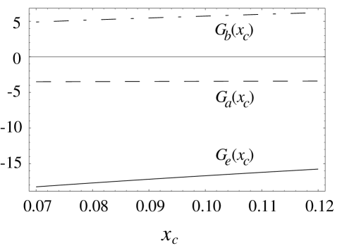
FIG. 6.: Variation of $G_{\{a,b,e\}}$ with $x_{c}$. The dashed line is $G_{a}(x_{c})$, the dash-dotted line is $G_{b}(x_{c})$, and the solid line is $G_{e}(x_{c})$.

Likewise, $G_{b}=G_{d}$ and can be extracted from the computation of perturbative QCD corrections to the polarization operator of vector and axial currents [11, 22],

$$G_{b}(x_{c}) = \frac{1}{48f(x_{c})}\Bigl{\{}(1-x_{c})(18-476x_{c}-539x_{c}^{2}+75x_{c}^{3})$$ (A27)

$$\qquad\qquad\mbox{}+4x_{c}^{2}(36+8x_{c}-x_{c}^{2})(\pi^{2}-3\ln^{2}x_{c})$$

$$\qquad\qquad\mbox{}-2(1-x_{c}^{2})\Big{(}31-320x_{c}+31x_{c}^{2}-12(1-8x_{c}+x_{c}^{2})\ln x_{c}\Big{)}\ln(1-x_{c})$$

$$\qquad\qquad\mbox{}-2x_{c}(132+90x_{c}-308x_{c}^{2}+31x_{c}^{3})\ln x_{c}$$

$$\qquad\qquad\mbox{}+24\bigl{(}2-16x_{c}-36x_{c}^{2}+8x_{c}^{3}-x_{c}^{4}+12x_{c}^{2}\ln x_{c}\bigr{)}\,{\rm Li}_{2}(x_{c})$$

$$\qquad\qquad\mbox{}+864x_{c}^{2}\Big{(}\zeta(3)-{\rm Li}_{3}(x_{c})\Big{)}\Bigr{\}}\,.$$

Hence $G_{e}$ is the only new quantity which needs to be computed. We have done this numerically, modifying a subroutine given to us by P. Ball [6]. Since each of $G_{a},G_{b},G_{c}$, and $G_{d}$ is related to a physical process, the individual classes of the diagrams are gauge invariant and free of infrared singularities. We present plots of $G_{i}(x_{c})$ in Fig. 6, with $\mu=m_{b}$ and $m_{b}-m_{c}=3.35\,$GeV. We see that the dependence on the quark masses is not very strong.

To obtain the radiative correction to $R_{1}$, the results of this calculation must be combined with the one-loop result for $b\to c\ell\bar{\nu}$ [23]. For the denominator of $\delta_{2}$, we use the result of Ref. [6]. The radiative corrections to the two observables are plotted in Fig. 1 of the text.

REFERENCES

[1] A.F. Falk and A.A. Petrov, hep-ph/9903518,
JHU–TIPAC–99003.
[2] S.J. Brodsky, G.P. Lepage and P.B. MacKenzie,
Phys. Rev. D 28, 228 (1983).
[3] S. Marka, presentation VB09.10 at the
April 1999 Centennial Meeting of the APS;
M. Bishai et
al. (CLEO Collaboration), Phys. Rev. D57, 3847 (1998).
[4] K. Kinoshita, private communication.
[5] G. Altarelli and L. Maiani, Phys. Lett. 52B, 351 (1974);
M.K. Gaillard and B.W. Lee, Phys. Rev. Lett.
33, 108 (1979);
F.G. Gilman and M.B. Wise, Phys. Rev.
D 20, 2392 (1979).
[6] E. Bagan et al., Nucl. Phys. B432,
3 (1994).
[7] B.H. Smith and M.B. Voloshin, Phys. Lett. B 340, 176 (1994).
[8] M. Lu, M. Luke, M. J. Savage and B. H. Smith,
Phys. Rev. D 55, 2827 (1997).
[9] M. Luke, M.J. Savage and M.B. Wise,
Phys. Lett. B 343, 329 (1995); ibid.345, 301
(1995).
[10] A.F. Falk and M. Neubert, Phys. Rev. D
47, 2965 (1993);
A.V. Manohar and M.B. Wise, Phys. Rev.
D 49, 1310 (1994);
I.I. Bigi et al., Phys. Rev.
Lett. 71, 496 (1993).
[11] L.J. Reinders et al., Phys. Lett. 97B, 257 (1980); ibid.103B, 63 (1981).
[12] A.F. Falk et al., Phys. Lett. B 326,
145 (1994);
L. Koyrakh, Phys. Rev. D 49, 3379 (1994).
[13] I.I. Bigi et al., Phys. Lett. B 293, 430 (1992); Erratum, ibid, 297, 477 (1993).
[14] E. Eichten and B. Hill, Phys. Lett. B 243,
427 (1990);
A.F. Falk, B. Grinstein and M. Luke, Nucl. Phys.
B357, 185 (1991).
[15] M. Neubert and C. Sachrajda, Nucl. Phys.
B483, 339 (1997).
[16] M. Di Pierro and C.T. Sachrajda
(UKQCD Collaboration), hep-lat/9809083.
[17] V. Chernyak, Nucl. Phys. B457, 96 (1995).
[18] M.S. Baek et al.
Phys. Rev. D 57, 4091 (1998).
[19] H. Cheng and K. Yang, Phys. Rev. D 59,
014011 (1999).