bla

Electromagnetic Corrections to $K\to\pi\pi$ I – Chiral Perturbation Theory

Vincenzo Cirigliano^a, John F. Donoghue^b and Eugene Golowich^b

^a Dipartimento di Fisica dell’Università and I.N.F.N.

Via Buonarroti,2 56100 Pisa (Italy)

vincenzo@het.phast.umass.edu

^b Department of Physics and Astronomy

University of Massachusetts

Amherst MA 01003 USA

donoghue@het.phast.umass.edu

gene@het.phast.umass.edu

An analysis of electromagnetic corrections to the (dominant) octet $K\to\pi\pi$ hamiltonian using chiral perturbation theory is carried out. Relative shifts in amplitudes at the several per cent level are found.

1 Introduction

In this paper, we present a formal analysis of electromagnetic (EM) radiative corrections to $K\to\pi\pi$ transitions. Only EM corrections to the dominant octet nonleptonic hamiltonian are considered. Such corrections modify not only the original $\Delta I=1/2$ amplitude but also induce $\Delta I=3/2,5/2$ contributions as well. By the standards of particle physics, this subject is very old [2]. Yet, there exists in the literature no satisfactory theoretical treatment. This is due largely to complications of the strong interactions at low energy. Fortunately, the modern machinary of the Standard Model, especially the method of chiral lagrangians, provides the means to perform an analysis which is both correct and structurally complete. That doing so requires no fewer than eight distinct chiral langrangians is an indication of the complexity of the undertaking.

There is, however, a problem with the usual chiral lagrangian methodology. The cost of implementing its calculational scheme is the introduction of many unknown constants, the finite counterterms associated with the regularization of divergent contributions. As regards EM corrections to nonleptonic kaon decay, it is impractical to presume that these many unknowns will be inferred phenomenologically in the reasonably near future, or perhaps ever. As a consequence, in order to obtain an acceptable phenomenological description, it will be necessary to proceed beyond the confines of strict chiral perturbation theory. In a previous publication [3], we succeeded in accomplishing this task in a limited context, $K^{+}\to\pi^{+}\pi^{0}$ decay in the chiral limit. We shall extend this work to a full phenomenological treatment of the $K\to\pi\pi$ decays in the next paper [4] of this series.

The proper formal analysis, which is the subject of this paper, begins in Sect. 2 where we briefly describe the construction of $K\to\pi\pi$ decay amplitudes in the presence of electromagnetic corrections. In Section 3, we begin to implement the chiral program by specifying the collection of strong and electroweak chiral lagrangians which bear on our analysis. The calculation of $K\to\pi\pi$ decay amplitudes is covered in Section 4 and our concluding remarks appear in Section 5.

Figure 1: Some electromagnetic contributions.

2 Electromagnetism and the $K\to\pi\pi$ Amplitudes

There are three physical $K\to\pi\pi$ decay amplitudes,

$${\cal A}_{K^{0}\to\pi^{+}\pi^{-}}\equiv{\cal A}_{+-}\ ,\qquad{\cal A}_{K^{0}\to\pi^{0}\pi^{0}}\equiv{\cal A}_{00}\ ,\qquad{\cal A}_{K^{+}\to\pi^{+}\pi^{0}}\equiv{\cal A}_{+0}\ \ .$$ (1)

We consider first these amplitudes in the limit of exact isospin symmetry and then identify which modifications must occur in the presence of electromagnetism.

In the $I=0,2$ two-pion isospin basis, it follows from the unitarity constraint that

$${\cal A}_{+-}\ = \ A_{0}e^{i\delta_{0}}+\sqrt{1\over 2}A_{2}e^{i\delta_{2}}\ \ ,$$

$${\cal A}_{00}\ = \ A_{0}e^{i\delta_{0}}-\sqrt{2}A_{2}e^{i\delta_{2}}\ \ ,$$ (2)

$${\cal A}_{+0}\ = \ {3\over 2}A_{2}e^{i\delta_{2}}\ \ .$$

The phases $\delta_{0}$ and $\delta_{2}$ are just the $I=0,2$ pion-pion scattering phase shifts (Watson’s theorem), and in a CP-invariant world the moduli $A_{0}$ and $A_{2}$ are real-valued. The large ratio $A_{0}/A_{2}\simeq 22$ is associated with the $\Delta I=1/2$ rule.

When electromagnetism is turned on, several new features appear:

1. Charged external legs experience mass shifts (cf Fig. 1(a)).

2. Photon emission (cf Fig. 1(b)) occurs off charged external legs. This effect is crucial to the cancelation of infrared singularities.

3. Final state coulomb rescattering (cf Fig. 1(c)) occurs in $K^{0}\to\pi^{+}\pi^{-}$.

4. There are structure-dependent hadronic effects, hidden in Fig. 1 within the large dark vertices. In this paper, we consider the leading contributions (see Fig. 2) which arise from corrections to the $\Delta I=1/2$ hamiltonian.

5. There will be modifications of the isospin symmetric unitarity relations and thus extensions of Watson’s theorem.

Any successful explanation of EM corrections to $K\to\pi\pi$ decays must account for all these items.

An analysis [5] of the unitarity constraint which allows for the presence of electromagnetism yields

$${\cal A}_{+-} = \left(A_{0}+\delta A_{0}^{\rm em}\right)e^{i(\delta_{0}+\gamma_{0})}+{1\over\sqrt{2}}\left(A_{2}+\delta A_{2}^{\rm em}\right)e^{i(\delta_{2}+\gamma_{2})}\ ,$$

$${\cal A}_{00} = \left(A_{0}+\delta A_{0}^{\rm em}\right)e^{i(\delta_{0}+\gamma_{0})}-\sqrt{2}\left(A_{2}+\delta A_{2}^{\rm em}\right)e^{i(\delta_{2}+\gamma_{2})}\ \ ,$$ (3)

$${\cal A}_{+0} = {3\over 2}\left(A_{2}+\delta A_{2}^{+{\rm em}}\right)e^{i(\delta_{2}+\gamma_{2}^{\prime})}\ \ ,$$

to be compared with the isospin invariant expressions in Eq. (2). This parameterization holds for the IR-finite amplitudes, whose proper definition is discussed later in Sect. 4.3. Observe that the shifts $\delta A_{2}^{+{\rm em}}$ and $\gamma_{2}^{\prime}$ in ${\cal A}_{+0}$ are distinct from the corresponding shifts in ${\cal A}_{+-}$ and ${\cal A}_{00}$. This is a consequence of a $\Delta I=5/2$ component induced by electromagnetism. In particular, the $\Delta I=5/2$ signal can be recovered via

$${\cal A}_{5/2}={\sqrt{2}\over 5}\left[{\cal A}_{+-}-{\cal A}_{00}-\sqrt{2}{\cal A}_{+0}\right]\ \ .$$ (4)

Figure 2: Leading electromagnetic correction to $K\to\pi\pi$.

3 Chiral Lagrangians

The preceding section has dealt with aspects of the $K\to\pi\pi$ decays which are free of hadronic complexities. In this section and the next, we use chiral methods to address these structure-dependent contributions. The implementation of chiral symmetry via the use of chiral lagrangians provides a logically consistent framework for carrying out a perturbative analysis.

In chiral perturbation theory, the perturbative quantities of smallness are the momentum scale $p^{2}$ and the mass scale $\chi=2B_{0}{\bf m}$, where ${\bf m}$ is the quark mass matrix. In addition, we work to first order in the electromagnetic fine structure constant $\alpha$,

$${\cal A}_{i}={\cal A}_{i}^{(0)}+\alpha{\cal A}_{i}^{(1)}+\dots\ \ .$$ (5)

Our goal is to determine the ${\cal O}(\alpha)$ components $\alpha{\cal A}_{i}^{(1)}$. The fine structure constant thus represents a second perturbative parameter, and we consider contributions of chiral orders ${\cal O}(e^{2}p^{0})$ and ${\cal O}(e^{2}p^{2})$,

$$\alpha{\cal A}_{i}^{(1)}\ \equiv\ {\cal A}_{i}^{(e^{2}p^{0})}+{\cal A}_{i}^{(e^{2}p^{2})}\ \ .$$ (6)

We shall restrict our attention to just the leading electromagnetic corrections to the $K\to\pi\pi$ amplitudes. Since the weak $\Delta I=1/2$ amplitude is very much larger than the $\Delta I=3/2$ amplitude, our approach is to consider only electromagnetic corrections to $\Delta I=1/2$ amplitudes. As a class these arise via processes contained in Fig. 2, where $g_{8}$ is the octet weak coupling defined below in Eq. (13).

We adopt standard usage in our chiral analysis, taking the matrix $U$ of light pseudoscalar fields and its covariant derivative $D_{\mu}U$ as

$$U\equiv\exp(i\lambda_{k}\Phi_{k}/F_{\pi})\ \ (k=1,\dots,8)\ ,\qquad D_{\mu}U\equiv\partial_{\mu}U+ie[Q,U]A_{\mu}\ \ ,$$ (7)

where $Q=~{}diag~{}(2/3,-1/3,-1/3)$ is the quark charge matrix and $A_{\mu}$ is the photon field. The remainder of this section summarizes the eight distinct effective lagrangians (strong, electromagnetic, weak and electroweak) needed in the analysis.

3.1 Strong and Electromagnetic Lagrangians

In the $\Delta S=0$ sector, we shall employ the strong/electromagnetic lagrangian

$${\cal L}^{(2)}_{\rm str}={F^{2}_{0}\over 4}\,{\rm Tr}\,\left(D_{\mu}UD^{\mu}U^{\dagger}\right)+{F^{2}_{0}\over 4}\,{\rm Tr}\,\left(\chi U^{\dagger}+U\chi^{\dagger}\right)\ ,$$ (8)

where $F$ is the pseudoscalar meson decay constant in lowest order. ${\cal L}^{(2)}_{\rm str}$ will be used to produce ${\cal O}(e^{0}p^{2})$ and ${\cal O}(e^{1}p^{1})$ vertices in our calculation.

The lagrangian ${\cal L}^{(2)}_{\rm str}$ will generate (via tadpole diagrams) strong self-energy effects on the external legs in the $K\to\pi\pi$ transitions. In order to regularize these divergent contributions, one employs the lagrangian [6] ${\cal L}^{(4)}_{\rm str}$. It is not necessary to write out this well-known set of operators, but simply to point out that the resulting wave function renormalization factors $Z_{\pi}$ and $Z_{K}$ obey

$${1\over F_{\pi}^{2}F_{K}}\ =\ {Z_{\pi}\sqrt{Z_{K}}\over F^{3}}\ \ ,$$ (9)

up to logarithms. This explains the presence of $F_{\pi}^{2}F_{K}$ in formulae such as Eqs. (22),(26) in Section 4.

Two other nonweak effective lagrangians enter the calculation. The first is associated with electromagnetic effects at chiral order ${\cal O}(e^{2}p^{0})$,

$${\cal L}_{\rm ems}^{(0)}=g_{\rm ems}\,{\rm Tr}\,\left(QUQU^{\dagger}\right)\ \ ,$$ (10)

where the coupling $g_{\rm ems}$ is fixed (in lowest chiral order) from the pion electromagnetic mass splitting,

$$g_{\rm ems}={F_{\pi}^{2}\over 2}~{}\delta M_{\pi}^{2}\ \ .$$ (11)

The second extends the description to chiral order ${\cal O}(e^{2}p^{2})$. We need only the following subset of the lagrangian given in Ref. [7],

$${\cal L}_{\rm ems}^{(2)}=F^{2}e^{2}\bigg{[}\kappa_{1}\,{\rm Tr}\,\left(D_{\mu}UD^{\mu}U^{\dagger}\right)\cdot\,{\rm Tr}\,Q^{2}$$

$$\phantom{xxxxxxxx}~{}+\kappa_{2}\,{\rm Tr}\,\left(D_{\mu}UD^{\mu}U^{\dagger}\right)\cdot\,{\rm Tr}\,\left(QUQU^{\dagger}\right)$$

$$\phantom{xxxxxxxx}~{}+\kappa_{3}\left(\,{\rm Tr}\,\left(D_{\mu}U^{\dagger}QU\right)\cdot\,{\rm Tr}\,\left(D^{\mu}U^{\dagger}QU\right)\right.$$

$$\left.\phantom{xxxxxxxxxxxxx}+\,{\rm Tr}\,\left(D_{\mu}UQU^{\dagger}\right)\cdot\,{\rm Tr}\,\left(D^{\mu}UQU^{\dagger}\right)\right)$$

$$\phantom{xxxxxxxx}~{}+\kappa_{4}\,{\rm Tr}\,\left(D_{\mu}U^{\dagger}QU\right)\cdot\,{\rm Tr}\,\left(D^{\mu}UQU^{\dagger}\right)$$ (12)

$$\phantom{xxxxxxxx}~{}+\kappa_{5}\left(\,{\rm Tr}\,\left(D_{\mu}U^{\dagger}D_{\mu}UQ\right)+\,{\rm Tr}\,\left(D_{\mu}UD^{\mu}U^{\dagger}Q\right)\right)$$

$$\phantom{xxxxxxxx}~{}+\kappa_{6}\,{\rm Tr}\,\left(D_{\mu}U^{\dagger}D^{\mu}UQU^{\dagger}QU+D_{\mu}UD^{\mu}U^{\dagger}QUQU^{\dagger}\right)\bigg{]}\ \ .$$

Although the finite parts of the coefficients $\kappa_{1},\dots,\kappa_{6}$ remain unconstrained, see however Refs. [8, 9, 10] for model determinations.

3.2 Weak Lagrangians

The $|\Delta S|=1$ octet lagrangian begins at chiral order $p^{2}$,

$${\cal L}_{8}^{(2)}\ =\ g_{8}\,{\rm Tr}\,\left(\lambda_{6}D_{\mu}UD^{\mu}U^{\dagger}\right)\ \ ,$$ (13)

with $g_{8}\simeq 6.7\cdot 10^{-8}~{}F_{\pi}^{2}$ fit [16] from $K\to\pi\pi$ decay rates. We use this to generate ${\cal O}(e^{0}p^{2})$, ${\cal O}(e^{1}p^{1})$ and ${\cal O}(e^{2}p^{0})$ vertices.

Two chiral lagrangians will serve to provide counterterms for removing divergent contributions. The first [11] is the octet $|\Delta S|=1$ lagrangian at chiral order $p^{4}$,

$${\cal L}_{8}^{(4)} = N_{5}\,{\rm Tr}\,\lambda_{6}\bigg{[}\left(U\chi^{\dagger}+\chi U^{\dagger}\right)\partial_{\mu}U\partial^{\mu}U^{\dagger}+\partial_{\mu}U\partial^{\mu}U^{\dagger}\left(U\chi^{\dagger}+\chi U^{\dagger}\right)\bigg{]}$$ (14)

$$+ N_{6}\,{\rm Tr}\,\lambda_{6}U\partial_{\mu}U^{\dagger}\cdot\,{\rm Tr}\,\left(\chi^{\dagger}\partial^{\mu}U-\chi\partial^{\mu}U^{\dagger}\right)$$

$$+ N_{7}\,{\rm Tr}\,\lambda_{6}\left(U\chi^{\dagger}+\chi U^{\dagger}\right)\cdot\,{\rm Tr}\,\partial_{\mu}U\partial^{\mu}U^{\dagger}$$

$$+ N_{8}\,{\rm Tr}\,\lambda_{6}\partial_{\mu}U\partial^{\mu}U^{\dagger}\cdot\,{\rm Tr}\,\left(U^{\dagger}\chi+\chi^{\dagger}U\right)$$

$$+ N_{9}\,{\rm Tr}\,\lambda_{6}\bigg{[}\partial_{\mu}U\partial^{\mu}U^{\dagger}\left(\chi U^{\dagger}-U\chi^{\dagger}\right)-\left(\chi U^{\dagger}-U\chi^{\dagger}\right)\partial_{\mu}U\partial^{\mu}U^{\dagger}\bigg{]}$$

$$+ N_{10}\,{\rm Tr}\,\lambda_{6}\left(U\chi^{\dagger}U\chi^{\dagger}+\chi U^{\dagger}\chi U^{\dagger}+U\chi^{\dagger}\chi U^{\dagger}\right)$$

$$+ N_{11}\,{\rm Tr}\,\lambda_{6}\left(U\chi^{\dagger}+\chi U^{\dagger}\right)\cdot\,{\rm Tr}\,\left(U^{\dagger}\chi+\chi^{\dagger}U\right)$$

$$+ N_{12}\,{\rm Tr}\,\lambda_{6}\left(U\chi^{\dagger}U\chi^{\dagger}+\chi U^{\dagger}\chi U^{\dagger}-U\chi^{\dagger}\chi U^{\dagger}\right)$$

$$+ N_{13}\,{\rm Tr}\,\lambda_{6}\left(U\chi^{\dagger}-\chi U^{\dagger}\right)\cdot\,{\rm Tr}\,\left(U\chi^{\dagger}-\chi U^{\dagger}\right)\ \ .$$

At present, little is known of the finite parts of the couplings $\{N_{k}\}$.

3.3 Electroweak Lagrangians

The $|\Delta S|=1$ lagrangian at chiral order ${\cal O}(e^{2}p^{0})$ is

$${\cal L}_{\rm emw}^{(0)}=g_{\rm emw}\,{\rm Tr}\,\left(\lambda_{6}UQU^{\dagger}\right)\ \ ,$$ (15)

where $g_{\rm emw}$ is an a priori unknown coupling constant. It has been calculated recently in Ref. [3],

$$g_{\rm emw}=\left(-0.62\pm 0.19\right)g_{8}\delta M_{\pi}^{2}\ \ .$$ (16)

We note in passing that despite the presence of just one charge matrix $Q$ the lagrangian of Eq. (15) indeed describes ${\cal O}(e^{2})$ effects. A second factor of $Q$ could be decomposed into a combination of the unit matrix and the $3\times 3$ matrix ${\hat{Q}}=~{}diag~{}(1,0,0)$. The contribution from ${\hat{Q}}$ would vanish, leaving the form of Eq. (15).

The second operator that we use to provide counterterm contributions is the $|\Delta S|=1$ lagrangian at chiral order ${\cal O}(e^{2}p^{2})$. In terms of the notation $L_{\mu}\equiv iU\partial_{\mu}U^{\dagger}$, we have

$${\cal L}_{emw}^{(2)}=e^{2}g_{8}\bigg{[}s_{1}\,{\rm Tr}\,\lambda_{6}[Q,L_{\mu}QL^{\mu}]_{+}$$

$$+s_{2}\,{\rm Tr}\,\lambda_{6}\left(QUQU^{\dagger}L_{\mu}L^{\mu}+L_{\mu}L^{\mu}UQU^{\dagger}Q\right)$$

$$+s_{3}\,{\rm Tr}\,\lambda_{6}[Q,L_{\mu}UQU^{\dagger}L^{\mu}]_{+}+s_{4}\,{\rm Tr}\,\lambda_{6}[L_{\mu},UQU^{\dagger}]_{+}\cdot\,{\rm Tr}\,UQU^{\dagger}L^{\mu}$$

$$+s_{5}\,{\rm Tr}\,\lambda_{6}\left(QUQU^{\dagger}\chi U^{\dagger}+U\chi^{\dagger}UQU^{\dagger}Q\right)$$

$$+s_{6}\,{\rm Tr}\,\lambda_{6}[\chi,U^{\dagger}]_{+}\cdot\,{\rm Tr}\,UQU^{\dagger}Q$$ (17)

$$+s_{7}\,{\rm Tr}\,\lambda_{6}\left(UQU^{\dagger}Q\chi U^{\dagger}+U\chi^{\dagger}QUQU^{\dagger}\right)$$

$$+s_{8}\,{\rm Tr}\,\left(\lambda_{6}\partial_{\mu}U\partial^{\mu}U^{\dagger}\right)\cdot\,{\rm Tr}\,Q^{2}$$

$$+s_{9}\,{\rm Tr}\,\left(\lambda_{6}\partial_{\mu}U\partial^{\mu}U^{\dagger}\right)\cdot\,{\rm Tr}\,UQU^{\dagger}Q\bigg{]}\ \ .$$

The first six operators in the above list appear in Ref. [12]. The remaining three are also required for our analysis. To our knowledge, none of the divergent or finite parts of the $\{s_{n}\}$ are yet known.

4 Calculation of Leading EM Corrections

The leading EM corrections arise from the processes of Fig. 1 and Fig. 2. Contributions to Fig. 2 occur in two distinct classes, those explicitly containing virtual photons (Fig. 3) and those with no explicit virtual photons (Fig. 4). The latter are induced by EM mass corrections and by insertions of $g_{\rm emw}$. In Figs. 3,4, the larger bold-face vertices are where the weak interaction occurs.

The integrals which occur in our chiral analysis are standard and already appear in the literature (e.g. see Ref. [13] or Ref. [14]). It suffices here to point out that all divergent parts of the one-loop integrals are ultimately expressible in terms of the $d$-dimensional integral

$$A(M^{2})\equiv\int d{\tilde{k}}~{}~{}{1\over k^{2}-M^{2}}=\mu^{d-4}\left[-2iM^{2}{\overline{\lambda}}-{iM^{2}\over 16\pi^{2}}\log\left({M^{2}\over\mu^{2}}\right)+\dots\right]\ \ ,$$ (18)

where $d{\tilde{k}}\equiv d^{d}k/(2\pi)^{d}$ is the integration measure, $\mu$ is the scale associated with dimensional regularization and ${\overline{\lambda}}$ is the singular quantity

$${\overline{\lambda}}\equiv{1\over 16\pi^{2}}\left[{1\over d-4}-{1\over 2}\left(\log{4\pi}-\gamma+1\right)\right]\ \ .$$ (19)

Each amplitude in the discussion to follow will be expressed as a sum of a finite contribution and a singular term containing ${\overline{\lambda}}$.

Figure 3: Explicit photon contributions in $K^{+}\to\pi^{+}\pi^{0}$.

4.1 Summary of ${\cal O}(e^{2})$ Amplitudes

We begin with the ${\cal O}(e^{2}p^{0})$ amplitudes,

$${\cal A}_{+-}^{(e^{2}p^{0})}=-{\sqrt{2}\over F_{K}F_{\pi}^{2}}\left(g_{8}\delta M_{\pi}^{2}+g_{\rm emw}\right)~{},\quad{\cal A}_{00}^{(e^{2}p^{0})}=0~{},\quad{\cal A}_{+0}^{(e^{2}p^{0})}={{\cal A}_{+-}^{(e^{2}p^{0})}\over\sqrt{2}}~{}.$$ (20)

Although these have already been determined in Ref. [3], we include them here for the sake of completeness. They are finite-valued and require no regularization procedure.

Next come the amplitudes of order $e^{2}p^{2}$, expressed as

$${\cal A}_{i}^{(e^{2}p^{2})}={\cal A}_{i}^{\rm(expl)}+{\cal A}_{i}^{\rm(impl)}+{\cal A}_{i}^{\rm(ct)}\ \ .$$ (21)

The superscript ‘expl’ refers to Figs. 1(a),(c) and Fig. 3 where virtual photons are explicitly present, whereas superscript ‘impl’ refers to Fig. 4 where EM effects are implicitly present via EM mass splittings and $g_{\rm emw}$ insertions. The final term ${\cal A}^{\rm(ct)}$ is the counterterm amplitude.

4.1.1 Diagrams with Explicit Photons

We turn first to the class ${\cal A}^{\rm(expl)}$ of explicit photonic diagrams. For these contributions, it is consistent to take meson masses in the isospin limit. We find

$${F_{K}F_{\pi}^{2}\over\sqrt{2}g_{8}}{\cal A}_{+-}^{\rm(expl)}=\left(M_{K}^{2}-M_{\pi}^{2}\right)\cdot\alpha{B}_{+-}(m_{\gamma})$$

$$\phantom{xxxxx}+{\alpha\over 4\pi}\left[7M_{\pi}^{2}-3M_{K}^{2}\left(\ln{M_{\pi}^{2}\over\mu^{2}}+1\right)\right]-6\mu^{d-4}e^{2}M_{K}^{2}{\overline{\lambda}}\ \ ,$$

$${F_{K}F_{\pi}^{2}\over\sqrt{2}g_{8}}{\cal A}_{00}^{\rm(expl)}=0\ \ ,$$ (22)

$${F_{K}F_{\pi}^{2}\over g_{8}}{\cal A}_{+0}^{\rm(expl)}={\alpha\over 4\pi}M_{\pi}^{2}\left[7-3\left(\ln{M_{\pi}^{2}\over\mu^{2}}+1\right)\right]-6\mu^{d-4}e^{2}M_{\pi}^{2}{\overline{\lambda}}\ \ .$$

The quantity ${B}_{+-}$, which appears in the above expression for ${\cal A}_{+-}^{\rm(expl)}$, is associated with the processes of Figs. 1(a),(c). Due to such processes, the weak decay amplitudes ${\cal A}_{i}$ will develop infrared (IR) singularities in the presence of electromagnetism. To tame such behavior, an IR regulator is introduced and appears as a parameter in the amplitudes. For our work, this takes the form of a photon squared-mass $m_{\gamma}^{2}$. ${B}_{+-}$ is given by

$${B}_{+-}(m_{\gamma}^{2}) = {1\over 4\pi}\bigg{[}2a(\beta)\ln{M_{\pi}^{2}\over m_{\gamma}^{2}}+{1+\beta^{2}\over 2\beta}h(\beta)+2+\beta\ln{1+\beta\over 1-\beta}$$ (23)

$$\phantom{xxxxx}+i\pi\left({1+\beta^{2}\over\beta}\ln{M_{K}^{2}\beta^{2}\over m_{\gamma}^{2}}-\beta\right)\bigg{]}\ \ ,$$

where

$$\beta=(1-4M_{\pi}^{2}/M_{K}^{2})^{1/2}$$ (24)

and

$$a(\beta) = 1+{1+\beta^{2}\over 2\beta}\ln{1-\beta\over 1+\beta}\ \ ,$$

$$h(\beta) = \pi^{2}+\ln{1+\beta\over 1-\beta}\ln{1-\beta^{2}\over 4\beta^{2}}+2f\left({1+\beta\over 2\beta}\right)-2f\left({\beta-1\over 2\beta}\right)\ \ ,$$ (25)

$$f(x) = -\int_{0}^{x}dt~{}{1\over t}\ln|1-t|\ \ .$$

Notice that the function ${B}_{+-}$ is complex, and both its real and imaginary parts have a logarithmic singularity as $m_{\gamma}\rightarrow 0$. The solution to this problem is well known; in order to get an infrared-finite decay rate, one has to consider the process with emission of soft real photons, whose singularity will cancel the one coming from soft virtual photons. We shall be more explicit on this point in Sect. 4.3.

Figure 4: Diagrams without explicit photon contributions.

The amplitudes ${\cal A}_{+-}^{\rm(expl)}$ and ${\cal A}_{+0}^{\rm(expl)}$ each contain an additive divergent term (proportional to ${\overline{\lambda}}$) and also depend on the arbitrary scale $\mu$ introduced in dimensional regularization of loop integrals. Both these features will require the introduction of counterterms.

4.1.2 Diagrams without Explcit Photons

Next comes the class ${\cal A}^{\rm(impl)}$ of diagrams in Fig. 4 not containing explicit photons. For such contributions, one must be sure to include all possible effects of chiral order ${\cal O}(e^{2}p^{0})$ and ${\cal O}(e^{2}p^{2})$ and treat the various terms in a consistent manner. Thus for the contributions to Fig. 4, isospin-invariant meson masses are used in amplitudes involving ${\cal L}_{\rm emw}^{(0)}\times{\cal L}_{\rm str}^{(2)}$ and ${\cal L}_{\rm ems}^{(0)}\times{\cal L}_{8}^{(2)}$, whereas electromagnetic mass splittings appear in amplitudes involving ${\cal L}_{\rm str}^{(2)}\times{\cal L}_{8}^{(2)}$. We write the results as sums of complex-valued finite amplitudes ${\cal F}_{i}(\mu)$ and divergent parts, essentially the amplitudes ${\cal D}_{i}$,

$${\cal A}_{i}^{\rm(impl)}={\cal R}e~{}{\cal F}_{i}(\mu)+i{\cal I}m~{}{\cal F}_{i}(\mu)+\mu^{d-4}{\cal D}_{i}~{}{\overline{\lambda}}\ ,\qquad(i=+-,00,+0)\ \ .$$ (26)

The scale-dependence in ${\cal F}_{i}(\mu)$ comes entirely from its real part ${\cal R}e~{}{\cal F}_{i}(\mu)$.

We express the ${\cal R}e~{}{\cal F}_{i}$ in terms of dimensionless amplitudes $a_{i}^{\rm(impl)}$,

$${\cal R}e~{}{\cal F}_{i}(\mu)=\eta_{i}{g_{8}M_{K}^{2}\over F_{\pi}^{2}F_{K}}a_{i}^{\rm(impl)}(\mu)\ \ ,$$ (27)

with $\eta_{+-}=\eta_{00}=\sqrt{2}$, $\eta_{+0}=1$. Since the $a_{i}^{\rm(impl)}(\mu)$ coefficients have rather cumbersome analytic forms, we find it most convenient to express them in the compact form

$$a_{i}^{\rm(impl)}(\mu)=b_{i}^{\rm(M)}{\delta M_{\pi}^{2}\over F^{2}}+b_{i}^{\rm(g)}{g\over F^{2}}+\bigg{[}c_{i}^{\rm(M)}{\delta M_{\pi}^{2}\over F^{2}}+c_{i}^{\rm(g)}{g\over F^{2}}\bigg{]}\ln{\mu\over 1~{}{\rm GeV}}\ \ ,$$ (28)

where

$$g\ \equiv\ g_{\rm emw}/g_{8}\ \ .$$ (29)

The coefficients appearing in Eq. (28) are given in Table 1.

Table 1: Values of Coefficients in Eq. (29)
	$b_{i}^{\rm(M)}$	$b_{i}^{\rm(g)}$	$c_{i}^{\rm(M)}$	$c_{i}^{\rm(g)}$
$i=+-$	$0.0160$	$-0.0409$	$-0.0078$	$-0.0445$
$i=00$	$-0.0170$	$-0.0224$	$-0.0371$	$-0.0176$
$i=+0$	$-0.0265$	$-0.0220$	$-0.0419$	$-0.0357$

The finite functions also have imaginary parts ${\cal I}m~{}{\cal F}_{i}$ which arise entirely from the processes in Fig. 4(c). From direct calculation we find

$${F_{K}F_{\pi}^{2}F^{2}\over\sqrt{2}g_{8}}{\cal I}m~{}{\cal F}_{+-}=-{\beta\over 16\pi}\left[{M_{K}^{2}\over 2}\left(\delta M_{\pi}^{2}+g\right)\right.$$

$$\left.\phantom{xxxxxxxxxxxxxxxxxxxxx}+\left({1\over\beta^{2}}-2\right)\left(M_{K}^{2}-M_{\pi}^{2}\right)\delta M_{\pi}^{2}\right]\ ,$$

$${F_{K}F_{\pi}^{2}F^{2}\over\sqrt{2}g_{8}}{\cal I}m~{}{\cal F}_{00}=-{\beta\over 16\pi}\left(M_{K}^{2}-M_{\pi}^{2}\right)\left[\delta M_{\pi}^{2}+g\right.$$

$$\left.\phantom{xxxxxxxxxxxxxxxxxxxxx}+2{M_{K}^{2}-M_{\pi}^{2}\over\beta^{2}}{\delta M_{\pi}^{2}\over M_{K}^{2}}\right]\ ,$$ (30)

$${F_{K}F_{\pi}^{2}F^{2}\over g_{8}}{\cal I}m~{}{\cal F}_{+0}={\beta\over 32\pi}\left(M_{K}^{2}-2M_{\pi}^{2}\right)\left(\delta M_{\pi}^{2}+g\right)\ \ ,$$

where $\beta$ is defined in Eq. (24). As a check on our calculation, we have verified that the above results are identical to those obtained from unitarity.

The singular parts of ${\cal A}_{i}^{\rm(impl)}$ are embodied by the ${\cal D}$-functions,

$${F^{2}F_{K}F_{\pi}^{2}\over\sqrt{2}g_{8}}{\cal D}_{+-}=M_{K}^{2}\left[{1\over 2}\delta M_{\pi}^{2}+{13\over 2}g\right]+M_{\pi}^{2}\left[10\delta M_{\pi}^{2}+7g\right]\ \ ,$$

$${F^{2}F_{K}F_{\pi}^{2}\over\sqrt{2}g_{8}}{\cal D}_{00}=\left(M_{K}^{2}-M_{\pi}^{2}\right)\left[{19\over 3}\delta M_{\pi}^{2}+3g\right]\ \ ,$$ (31)

$${F^{2}F_{K}F_{\pi}^{2}\over g_{8}}{\cal D}_{+0}=M_{K}^{2}\left[{19\over 3}\delta M_{\pi}^{2}+{89\over 18}g\right]+M_{\pi}^{2}\left[4\delta M_{\pi}^{2}+{86\over 9}g\right]\ \ .$$

To arrive at the above, we have used both the correspondence between $\delta M_{\pi}^{2}$ and $g_{\rm ems}$ given in Eq. (11) and also the relation

$$M_{\pi^{\pm}}^{2}-M_{\pi^{0}}^{2}\ =\ M_{K^{+}}^{2}-M_{K^{0}}^{2}\ \ ,$$ (32)

in the evaluation of loop integrals. The latter follows from Dashen’s theorem [15] and is justified since terms violating Dashen’s theorem would begin to contribute at the higher chiral order $e^{2}p^{4}$.

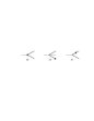
Figure 5: Counterterm contributions.

4.2 The Regularization Procedure

In order to cancel the singular ${\overline{\lambda}}$-dependence in the $K\to\pi\pi$ amplitudes, it is necessary to calculate all possible counterterm amplitudes which can contribute. These enter in a variety of ways, as shown in Fig. 5 where the small bold-face square denotes the counterterm vertex. For Figs. 5(a),(b) the counterterm vertex has $|\Delta S|=1$ whereas in Fig. 5(c) it has $\Delta S=0$.

4.2.1 Counterterm Amplitudes

Using the lagrangians ${\cal L}_{8}^{(4)}$, ${\cal L}_{\rm emw}^{(2)}$ and ${\cal L}_{\rm ems}^{(2)}$ we determine the counterterm amplitudes to be

$${F^{2}F_{K}F_{\pi}^{2}\over\sqrt{2}g_{8}}{\cal A}_{+-}^{\rm(ct)}=$$

$$\phantom{xxxxx}M_{K}^{2}\left(e^{2}F^{2}(X_{1}-4U_{1}-{8\over 3}U_{2})+\delta M_{\pi}^{2}(8N_{7}-4N_{8}-4N_{9})\right)$$

$$\phantom{xxxxx}+M_{\pi}^{2}\left(e^{2}F^{2}(X_{2}+4U_{1}+{8\over 3}U_{2})-\delta M_{\pi}^{2}(4N_{5}+8N_{7}+2N_{8})\right)\ \ ,$$

$${F^{2}F_{K}F_{\pi}^{2}\over\sqrt{2}g_{8}}{\cal A}_{00}^{\rm(ct)}=\left(M_{K}^{2}-M_{\pi}^{2}\right)e^{2}F^{2}\bigg{[}X_{00}-4U_{1}-{8\over 3}U_{2}-2U_{3}\bigg{]}\ ,$$ (33)

$${F^{2}F_{K}F_{\pi}^{2}\over g_{8}}{\cal A}_{+0}^{\rm(ct)}=M_{K}^{2}\left(e^{2}F^{2}X_{3}-\delta M_{\pi}^{2}(4N_{5}+4N_{8})\right)$$

$$\phantom{xxxxx}+M_{\pi}^{2}\left(e^{2}F^{2}X_{4}-\delta M_{\pi}^{2}(2N_{8}+4N_{9})\right)\ \ ,$$

where the $\{N_{i}\}$ are coefficients in the $|\Delta S|=1$ lagrangian ${\cal L}_{8}^{(4)}$ of Eq. (14), the $\{U_{i}\}$ are combinations of coefficients in the $\Delta S=0$ lagrangian ${\cal L}_{\rm ems}^{(2)}$ of Eq. (12),

$$U_{1}=\kappa_{1}+\kappa_{2}\ ,\quad U_{2}=\kappa_{5}+\kappa_{6}\ ,\quad U_{3}=-2\kappa_{3}+\kappa_{4}\ ,$$ (34)

and the $\{X_{i}\}$ are combinations of coefficients in the $|\Delta S|=1$ lagrangian ${\cal L}_{\rm emw}^{(2)}$ of Eq. (12),

$$X_{1} = -{4\over 9}s_{1}-{1\over 9}s_{2}+{2\over 9}s_{3}+{2\over 3}s_{5}-4s_{6}+{2\over 3}s_{7}+s_{8}+s_{9}\ \ ,$$

$$X_{2} = {4\over 9}s_{1}-{2\over 9}s_{2}+{4\over 9}s_{3}+{4\over 3}s_{5}+4s_{6}-{2\over 3}s_{7}-s_{8}-s_{9}\ \ ,$$

$$X_{3} = -{2\over 3}s_{1}-{1\over 3}s_{2}+{4\over 3}s_{4}+{2\over 3}s_{5}+{2\over 3}s_{7}\ \ ,$$ (35)

$$X_{4} = {2\over 3}s_{1}+{2\over 3}s_{3}-{4\over 3}s_{4}+{4\over 3}s_{5}-{2\over 3}s_{7}\ \ ,$$

$$X_{00} = {2\over 9}\left(s_{1}+s_{2}+s_{3}\right)+{2\over 3}s_{4}+s_{8}+s_{9}\ \ ,$$

4.2.2 Removal of Divergences

The counterterms themselves have finite and singular parts,

$$N_{i} = n_{i}\mu^{d-4}{\overline{\lambda}}+N_{i}^{(r)}(\mu)\ \ ,$$

$$U_{i} = u_{i}\mu^{d-4}{\overline{\lambda}}+U_{i}^{(r)}(\mu)\ \ ,$$ (36)

$$X_{i} = x_{i}\mu^{d-4}{\overline{\lambda}}+X_{i}^{(r)}(\mu)\ \ .$$

The coefficients $n_{i},u_{i}$ of the divergent parts of $N_{i},U_{i}$ have already been specified in the literature [11, 7] and hence the $\mu$-dependences of $N_{i}^{(r)}$, $U_{i}^{(r)}$ are known from the renormalization group equations. We infer the $x_{i}$ coefficients in this paper by canceling divergences in the ${\cal O}(e^{2}p^{2})$ amplitudes. Upon combining results obtained thus far, we find the new results

$$x_{00} = -{1\over 3}{\delta M_{\pi}^{2}\over e^{2}F^{2}}-3{g\over e^{2}F^{2}}\ \ ,$$

$$x_{1} = 3+{27\over 2}{\delta M_{\pi}^{2}\over e^{2}F^{2}}-{13\over 2}{g\over e^{2}F^{2}}\ \ ,$$

$$x_{2} = 3-18{\delta M_{\pi}^{2}\over e^{2}F^{2}}-7{g\over e^{2}F^{2}}\ \ ,$$ (37)

$$x_{3} = -{7\over 3}{\delta M_{\pi}^{2}\over e^{2}F^{2}}-{89\over 18}{g\over e^{2}F^{2}}\ \ ,$$

$$x_{4} = 6-2{\delta M_{\pi}^{2}\over e^{2}F^{2}}-{86\over 9}{g\over e^{2}F^{2}}\ \ ,$$

where we recall $g\equiv g_{\rm emw}/g_{8}$.

4.3 Removal of Infrared Singularities

Removal of the infrared divergence from the expression for the decay rate is achieved by taking into account the process ${K}^{0}\to\pi^{+}\pi^{-}(n\gamma)$. For soft photons, whose energy is below the detector resolution $\omega$, this process cannot be experimentally distinguished from ${K}^{0}\to\pi^{+}\pi^{-}$, so the observable quantity involves the inclusive sum over the $\pi^{+}\pi^{-}$ and $\pi^{+}\pi^{-}(n\gamma)$ final states.

At the order we are working, it is sufficient to consider just the emission of a single photon. The amplitude for the radiative decay is given in lowest order by

$$\left.{\cal A}_{+-\,\gamma}=e\frac{\sqrt{2}g_{8}}{F_{K}F^{2}_{\pi}}\,(M_{K}^{2}-M_{\pi}^{2})\,\left(\frac{\epsilon\cdot p_{+}}{q\cdot p_{+}}-\frac{\epsilon\cdot p_{-}}{q\cdot p_{-}}\right)\ \ ,\right.$$ (38)

where $\epsilon$ and $q$ are the polarization and momentum of the emitted photon.
The infrared-finite observable decay rate is

$$\left.\Gamma_{+-}(\omega)=\Gamma_{+-}\ +\ \Gamma_{+-\,\gamma}(\omega)\ \ \ \ ,\right.$$ (39)

where

$$\Gamma_{+-} = \frac{1}{2M_{K}}\,\int\,d\Phi_{+-}\ |{\cal A}_{+-}|^{2}\ \ ,$$ (40)

$$\Gamma_{+\,-\,\gamma}(\omega) = \frac{1}{2M_{K}}\,\int_{E_{\gamma}<\omega}\,d\Phi_{+\,-\,\gamma}\ |{\cal A}_{+\,-\,\gamma}|^{2}\ \ ,$$ (41)

and $d\Phi_{k}$ is the differential phase space factor for each process. The infrared divergent (IRD) part of $\Gamma_{+-}$ is seen to be

$$\left.\Gamma_{+-}^{\rm(IRD)}=\frac{1}{2M_{K}}\,\left[\frac{\sqrt{2}g_{8}}{F_{K}F^{2}_{\pi}}\,(M_{K}^{2}-M_{\pi}^{2})\right]^{2}\int\,d\Phi_{+-}\ \ 2\alpha\,{\cal R}e{B}_{+-}(m_{\gamma})\right.\ \ .$$ (42)

Equation (42) displays explicitly the singularity and shows that the imaginary part of ${B}_{+-}(m_{\gamma})$ has no observable effect at this order. This result has been shown to be true to all orders in $\alpha$ [17, 18]. For $\Gamma_{+\,-\,\gamma}(\omega)$ we get the following expression, up to terms of order $\omega/M_{K}$,

$$\Gamma_{+\,-\,\gamma}(\omega)=\frac{1}{2M_{K}}\,\left[\frac{\sqrt{2}g_{8}}{F_{K}F^{2}_{\pi}}\,(M_{K}^{2}-M_{\pi}^{2})\right]^{2}\int\,d\Phi_{+-}\,\ {I}_{+-}(m_{\gamma},\omega)\ \ ,$$ (43)

where

$${I}_{+-}(m_{\gamma},\omega)={\alpha\over\pi}\left[a(\beta)\ln\left({m_{\gamma}\over 2\omega}\right)^{2}+F(\beta)\right]\ \ ,$$ (44)

with

$$F(\beta)={1\over\beta}\ln{1+\beta\over 1-\beta}+{1+\beta^{2}\over 2\beta}\bigg{[}2f(-\beta)-2f(\beta)+f\left({1+\beta\over 2}\right)$$

$$\phantom{xxxxx}-f\left({1-\beta\over 2}\right)+{1\over 2}\ln{1+\beta\over 1-\beta}~{}\ln(1-\beta^{2})+\ln 2~{}\ln{1-\beta\over 1+\beta}\bigg{]}\ \ .$$ (45)

From these explicit expressions of ${B}_{+-}(\omega)$ and ${I}_{+-}(m_{\gamma},\omega)$ it is easy to see that the combination $2\alpha\,{\cal R}e{B}_{+-}(m_{\gamma})+{I}_{+-}(m_{\gamma},\omega)$ does not depend on the infrared regulator $m_{\gamma}$. However, this combination has a dependence on the experimental resolution $\omega$. To obtain a meaningful prediction therefore requires knowledge of the experimental treatment of soft photons. A careful discussion of this point will appear in Ref. [5].

A generalization of the above considerations beyond the order ${\cal O}(e^{2}p^{2})$ in ChPT leads to the following parameterization,

$$\Gamma_{+-}(\omega)=\frac{1}{2M_{K}}\,\int d\Phi_{+-}\ G_{+-}(\omega)~{}\big{|}{\cal A}_{+-}^{(0)}\,+\,\alpha\,{\cal A}_{+-}^{(1)}\big{|}^{2}\ \ ,$$ (46)

where to first order in $\alpha$,

$$G_{+-}(\omega)=1+2\alpha\,{\cal R}e{B}_{+-}(m_{\gamma})\,+\,{I}_{+-}\,(m_{\gamma},\omega)\ \ .$$ (47)

With the prescription of dropping the term proportional to ${B}_{+-}$ in the photonic loop contribution, the electromagnetic amplitude $\alpha{\cal A}_{+-}^{(1)}$ can be read from Eqs. (20),(22),(26),(33).

4.4 The Finite Amplitudes

The physical amplitudes will be complex-valued functions, as dictated by unitarity. The real parts are obtained by combining the finite loop amplitudes (Eq. (22) for ${\cal A}_{i}^{\rm(expl)}$ and Eqs. (27),(28) along with Table 1 for ${\cal A}_{i}^{\rm(impl)}$) with the counterterm amplitudes of Eq. (33),

$${\cal R}e~{}{\cal A}_{i}^{(e^{2}p^{2})}\ =\ \eta_{i}{g_{8}M_{K}^{2}\over F_{\pi}^{2}F_{K}}\left[{\cal R}e~{}a_{i}^{\rm(loop)}+a_{i}^{\rm(ct)}\right]\ \ .$$ (48)

In order to make the scale-dependence of ${\cal R}e~{}a_{i}^{\rm(loop)}$ explicit, we write

$${\cal R}e~{}a_{i}^{\rm(loop)}\ =\ b_{i}+c_{i}\ln{\mu\over 1~{}{\rm GeV}}\ \ .$$ (49)

Numerical determination of the above quantities will depend on $g_{8}$ (obtained from Ref. [16]), $\delta M_{\pi}^{2}$ and $g_{\rm emw}$ (given in Eq. (16)). We obtain the central values

$$\begin{array}[]{l}b_{+-}=11.8\cdot 10^{-3}\ ,\\ b_{00}=-0.5\cdot 10^{-3}\ ,\\ b_{+0}=-1.3\cdot 10^{-3}\ ,\end{array}\qquad\begin{array}[]{l}c_{+-}=7.1\cdot 10^{-3}\ ,\\ c_{00}=-3.9\cdot 10^{-3}\ ,\\ c_{+0}=-2.7\cdot 10^{-3}\ \ .\end{array}$$ (56)

The imaginary parts of the physical amplitudes can be either determined from unitarity or read off from Eqs. (26),(30). Of most interest is the EM shift in ${\cal A}_{2}$, as only it receives the ${\cal A}_{0}/{\cal A}_{2}$ ($\Delta I=1/2$) enhancement,

$$\delta({\cal I}m~{}{\cal A}_{2}^{\rm em}) = {\beta\over 32\pi}\left[{\cal A}_{2}^{(e^{2}p^{0})}{\cal T}_{2}^{(e^{0}p^{2})}+{\cal A}_{0}^{(e^{0}p^{2})}{\cal T}_{02}^{(e^{2}p^{0})}\right.$$ (57)

$$\left.\phantom{xxxxxxx}-{2\sqrt{2}\over 3\beta^{2}}~{}{\delta M_{\pi}^{2}\over M_{K}^{2}}{\cal A}_{0}^{(e^{0}p^{2})}{\cal T}_{2}^{(e^{0}p^{2})}\right]\ ,$$

where ${\cal T}_{2}^{(e^{0}p^{2})}$ and ${\cal T}_{02}^{(e^{2}p^{0})}$ are pion-pion T-matrix elements in the isospin basis. The above three contributions have physically distinct origins; the first involves the direct effect of electromagnetism on the $I=2$ decay amplitude, the second arises from final state scattering in which electromagnetism induces leakage from $I=0$ to $I=2$, and the third is due to the shift in two-pion phase space produced by the electromagnetic mass shift [5].

5 Final Results and Concluding Remarks

Despite the presence of many unknown finite counterterms, it is possible to apply the numerical results of Eq. (56) and obtain rough estimates of the EM corrections. The reasoning is that since the physical amplitudes are independent of the scale $\mu$, there must be compensating $\mu$-dependence between the chiral logarithms of Eq. (49) and the counterterms. Therefore the counterterms must be at least of the same order-of-magnitude as the chiral logs or even larger. We have adopted the operational procedure of assuming the counterterm contribution $a_{i}^{\rm(ct)}$ vanishes at the scale $\mu=M_{\rho}$, and we assign an uncertainty given by $\pm|c_{i}|$. This leads to the numerical values

$$\delta(A_{0}^{\rm em}) = \left(0.024\pm 0.026\right)\cdot 10^{-7}~{}M_{K^{0}}\ \ ,$$

$$\delta(A_{2}^{\rm em}) = \left(0.015\pm 0.022\right)\cdot 10^{-7}~{}M_{K^{0}}\ \ ,$$

$$\delta(A_{2}^{+{\rm em}}) = \left(-0.005\pm 0.005\right)\cdot 10^{-7}~{}M_{K^{0}}\ \ ,$$ (58)

$${\cal A}_{5/2} = \left(0.012\pm 0.016\right)\cdot 10^{-7}~{}M_{K^{0}}\ \ ,$$

with $A_{0}=(5.458\pm 0.012)\cdot 10^{-7}~{}M_{K^{0}}$ and $A_{2}=(0.2454\pm 0.010)\cdot 10^{-7}~{}M_{K^{0}}$. Specifically, for the EM shift $\delta(A_{2}^{+{\rm em}}/A_{2})$ calculated in Ref. [3], we now have the extended result

$${\delta(A_{2}^{+{\rm em}})\over A_{2}}\ =\ -\left(2.0\pm 2.2\right)~{}\%\ \ .$$ (59)

If one allows for the uncertainty in $g_{\rm emw}$ in addition to those in the counterterm values, we find

$${\delta(A_{2}^{+{\rm em}})\over A_{2}}\ =\ -\left(2.0^{+4.0}_{-2.2}\right)~{}\%\ \ .$$ (60)

In the numerical findings of Eqs. (58)-(60), the error bars are seen to be almost as large or larger than the signal. In our opinion, this is the best that one can do within a strict chiral perturbation theory approach.

Our results illustrate several general features:

1. Since the central values of the amplitudes have $\delta A_{2}^{em}\neq\delta A_{2}^{+em}$, the electromagnetic loop corrections are seen to produce $\Delta I=5/2$ effects, although the uncertainties of the counterterm values overwhelms the numerical result.

2. A phenomenological analysis [19] based on $S$-wave pion-pion scattering lengths and forward dispersion relations gives $\delta_{0}-\delta_{2}=(42\pm 4)^{o}$. Yet an isospin analysis of $K\to\pi\pi$ decays yields $\delta_{0}-\delta_{2}=(56.7\pm 3.9)^{o}$. Presumably this difference of nearly $15^{o}$ can be reconciled by subtracting EM effects from the $K\to\pi\pi$ decays. The main EM shift should be in $\delta_{2}$ as only this angle experiences a $\Delta I=1/2$ enhancement. Using Eq. (57) to calculate the angle $\gamma_{2}$ of Eq. (3), we find

   $$\gamma_{2}={{\cal A}_{0}^{(e^{0}p^{2})}\over{\cal A}_{2}^{(e^{0}p^{2})}}\cdot{\beta\over 32\pi}\left[{\cal T}_{02}^{(e^{2}p^{0})}-{2\sqrt{2}\over 3\beta^{2}}~{}{\delta M_{\pi}^{2}\over M_{K}^{2}}~{}{\cal T}_{2}^{(e^{0}p^{2})}\right]\simeq 4.5^{o}\ .$$ (61)

   This evaluation, valid at order $e^{2}p^{0}$, is seen to worsen the discrepancy between the two determinations. To reveal the explanation behind this puzzle requires more work. [5]

3. Finally, the most important implication of these estimates is that the electromagnetic shifts in $A_{2}$ are not large, being only a few percent. Naive estimates allow the possibility that this shift could be much larger, perhaps even being a major portion of $A_{2}$. Our previous work at the leading order in the chiral expansion yielded a small effect. One motivation of the present calculation was to see if the next order effects upset this conclusion. Our estimates show that the natural size of the shift in $A_{2}$ remains at the few percent level.

This has been a complicated calculation with many different lagrangians, describing different aspects of electromagnetic physics, required to obtain the full effect. These include explicit photon loops, mass shifts in the mesons propagating in loops and the short-distance electroweak interaction. The chiral power counting was crucial in sorting out which effects must be included for a consistent calculation. The resulting structure is universal and model independent. However, it is a prelude to more fully predictive applications, as there remain unknown low energy constants which are not predicted by chiral symmetry alone. Different models can be used to estimate the renormalized constants which appear in the chiral lagrangians, and these model predictions can then be readily translated into the physical amplitudes through the use of our calculation. In a following publication, we attempt to describe the extent that this may be accomplished using dispersive techniques to match long and short distance physics [4].

The research described here was supported in part by the National Science Foundation. One of us (V.C.) acknowledges support from M.U.R.S.T. We thank John Belz for a useful communication.

References

[1]Calculation of Some Selected Isospin-Breaking
Observales in the Standard Model, C. Wolfe, Ph.D.thesis,
Univ. of Toronto (1999) unpublished.
[2] For example, see F. Abbud, B.W. Lee and C.N. Yang,
Phys. Rev. Lett. 18 (1967) 980; A.A. Belavin and I.M. Narodetskii,
Sov. J. Nucl. Phys. 8 (1968) 568; A. Neveu and J. Scherk,
Phys. Lett. B27 (1968) 384; A.A. Bel’kov and V.V. Kostyuhkin,
Sov. J. Nucl. Phys. 51 (1989) 326.
[3] V. Cirigliano, J.F. Donoghue
and E. Golowich, Phys. Lett. B450 (1999) 241.
[4]Electromagnetic Corrections
to II – Dispersive Matching,
V. Cirigliano, J.F. Donoghue and E. Golowich, hep-ph/9909374.
[5] Final State Phases in
the Presence of Electromagnetism, V. Cirigliano, J.F. Donoghue
and E. Golowich, in preparation.
[6] J. Gasser and H. Leutwyler, Nucl. Phys.
B250 (1985) 465.
[7] R. Urech, Nucl. Phys. B433 (1995) 234.
[8] J. Bijnens and J. Prades, Nucl. Phys.
B490 (1997) 239.
[9] R. Baur and R. Urech, Nucl. Phys.
B499 (1997) 319.
[10] B. Moussallam, Nucl. Phys.
B504 (1997) 381.
[11] G. Ecker, J. Kambor, and D. Wyler,
Nucl. Phys. B394 (1993) 101.
[12] E. de Rafael, Nucl. Phys.
7A (Proc. Suppl.) (1989) 1.
[13] J. Gasser and H. Leutwyler, Ann. Phys. 158
(1984) 142.
[14] E. Golowich and J. Kambor, Nucl. Phys.
B447, (1995) 373.
[15] R. Dashen, Phys. Rev. 183, (1969) 1245.
[16] J. Kambor, J. Missimer and D. Wyler,
Phys. Lett. B261 (1991) 496.
[17] S. Weinberg, Phys. Rev. B140 (1965) 516.
[18] D.R. Yennie, S.C. Frautschi and H. Suura,
Ann. Phys. 13 (1961) 379.
[19] E. Chell and M.G. Olsson, Phys. Rev. D48
(1993) 4076.