Terrestrial Neutrino Oscillations Illustrated  

Observations of atmospheric neutrinos offer compelling evidence that neutrinos have mass and do oscillate. Preliminary data are compatible with maximal $\nu_{\mu}$–$\nu_{\tau}$ mixing, but not with pure $\nu_{\mu}$–$\nu_{e}$ mixing. In a general three-family scenario with just one relevant squared-mass difference, atmospheric neutrino oscillations involve two mixing angles. The special cases mentioned above are not favored by convincing theoretical arguments. As more precise data are accumulated, both at Superkamiokande and at proposed or ongoing long-baseline experiments, it will become feasible and desirable to measure both angles. To this end, we offer a brief portfolio of illustrations from which the qualitative effects of the two mixing angles on various observable quantities can be discerned.

Observations of atmospheric and solar neutrinos suggest that neutrinos have mass and are subject to flavor oscillations. These oscillations may be described in terms of three chiral neutrinos with squared-mass differences $\Delta_{ij}\equiv|m_{i}^{2}-m_{j}^{2}|$ satisfying:

$${\Delta_{13}\simeq\Delta_{23}\simeq 10^{-3}\;{\rm eV^{2}}\,,\quad\ {\rm and}\quad\ \Delta_{12}\leq 10^{-5}\;{\rm eV^{2}}\,.}$$ (1)

The smaller difference $\Delta_{12}$ is relevant to solar neutrino oscillations, but it hardly affects oscillations of atmospheric neutrinos or of neutrinos to be studied at long-baseline experiments. These ‘terrestrial oscillations’ involve the larger squared-mass difference. They depend on two mixing angles, which we denote by $\theta_{1}$ and $\theta_{2}$, parametrizing the decomposition of the mass eigenstate $\nu_{3}$ into lepton flavor eigenstates:

$$\nu_{3}=s_{2}\,\nu_{e}+s_{1}c_{2}\,\nu_{\mu}+c_{1}c_{2}\,\nu_{\tau}$$ (2)

where $s_{i}$ and $c_{i}$ stand for sines and cosines of $\theta_{i}$. The relevant flavor-transition probabilities are:

$$\begin{array}[]{r@{\;}l}P(\nu_{\mu}\rightarrow\nu_{\tau})\simeq&4B(E)\,s_{1}^{2}c_{1}^{2}c_{2}^{4}\,,\qquad P(\nu_{e}\leftrightarrow\nu_{\mu})\simeq 4B(E)\,s_{1}^{2}s_{2}^{2}c_{2}^{2}\,,\\ &P(\nu_{e}\rightarrow\nu_{\tau})\simeq 4B(E)\,c_{1}^{2}s_{2}^{2}c_{2}^{2}\,,\\ \end{array}$$ (3)

where

$${B\equiv\sin^{2}{(\Delta_{13}R/4E)}\,,}$$ (4)

with $E$ the neutrino energy and $R$ its flight length. These results are familiar [1] and have been used to perform extensive analyses of available data [1, 2]. Our very modest purpose in this note is simply to exhibit how various observables depend on the two mixing angles.

We begin by considering atmospheric neutrino oscillations. Let $N_{\mu}$ and $N_{e}$ be the fluxes of $e$-like and $\mu$-like events that would be seen at a given site and direction were there no oscillations. The observed (primed) fluxes will be:

$$\begin{array}[]{r@{\;}l}N_{\mu}^{\prime}&=\big{(}1-4B\,s_{1}^{2}c_{2}^{2}(1-s_{1}^{2}c_{2}^{2})\big{)}\,N_{\mu}+4B\,s_{1}^{2}s_{2}^{2}c_{2}^{2}\,N_{e}\,,\\ N_{e}^{\prime}&=(1-4B\,s_{2}^{2}c_{2}^{2})\,N_{e}+4B\,s_{1}^{2}s_{2}^{2}c_{2}^{2}\,N_{\mu}\,.\\ \end{array}$$ (5)

To develop a feel for the import of these equations, we examine them in following simple limit: We use the approximation $N_{\mu}=2N_{e}$ and replace $B$ by its time and energy averaged value of 1/2. With these substitutions, the often-considered ratio of ratios becomes:

$${R\equiv(N_{\mu}^{\prime}/N_{e}^{\prime})/(N_{\mu}/N_{e})={1-2s_{1}^{2}c_{2}^{2}+2s_{1}^{4}c_{2}^{4}+s_{1}^{2}s_{2}^{2}c_{2}^{2}\over 1+4s_{1}^{2}s_{2}^{2}c_{2}^{2}-2s_{2}^{2}c_{2}^{2}}\,,}$$ (6)

a quantity that can vary within the interval $2\geq R\geq 0.5$. The observations are compatible with a value of $R$ near its lower bound. Indeed, that bound may be achieved at just two points: with maximal $\nu_{\mu}$–$\nu_{\tau}$ mixing ($s_{1}^{2}=1/2,\ s_{2}^{2}=0$), or with maximal $\nu_{\mu}$–$\nu_{e}$ mixing ($s_{1}^{2}=1,\ s_{2}^{2}=1/2$), the latter possibility being strongly disfavored. To exhibit the dependence of this ratio on other values of the mixing angles, we show contour plots for $R$ in figure 1.

The acceptances and biases of $e$-like and $\mu$-like events at SuperKamiokande may not be the same. Thus, when adequate data is available, it may be desirable to study their angular distributions separately. To this end, we present figures 2 and 3. We note in passing that SuperKamiokande data [3] may suggest a small up/down asymmetry of $e$-like events, and correspondingly, a non-zero value of $s_{2}$. The observables displayed in figures 1–3 are independent of the overall flux of atmospheric neutrinos, which is presently rather uncertain. Figure 4 shows the effect of oscillations on this quantity. If the flux uncertainty can be substantially reduced, the event rate may provide a useful constraint on the mixing angles.

At least two long baseline experiments will shed further light on the neutrino squared-mass difference and the two mixing angles: the ongoing K2K experiment and the approved Minos experiment. Figure 5 shows how the ratio of $e$-like events ($M_{e}$) to all observed events ($M_{\mu}+M_{e}$) depends on $\theta_{i}$. (Here we assume that the beam is pure $\nu_{\mu}$. In fact, there will be a 1–2% admixture of $\nu_{e}$, but this will be measured at the near detector.) An observed excess of $e$-like events would prove that $s_{2}\neq 0$ and thus, that all three flavors participate in the oscillations. Figure 6 shows the ratio of the actual event rate ($M_{\mu}+M_{e}$) to what it would be in the absence of oscillations—a quantity that would be useful only if the neutrino beam is precisely directed toward its distant target. Figures 5 and 6 must be taken with a grain of salt: the replacement of $B(E)$ by its $R/E$ average is not justified for either experiment. Our illustrations are intended solely as guides to the mind.

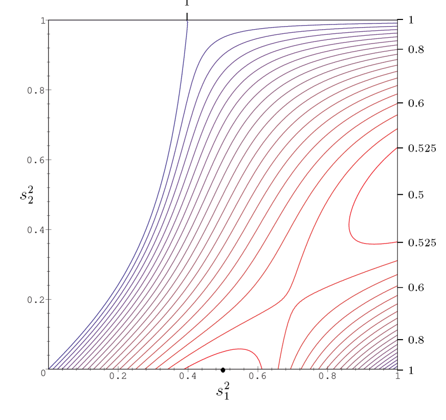
Figure 1: The ratio of ratios of atmospheric neutrino fluxes, $R\equiv(N_{e}^{\prime}N_{\mu}/N_{\mu}^{\prime}N_{e})$ (shown from $1/2$ to $1$ with contour spacing of 0.025). Note the shallow valley connecting the two points at which $R$ assumes its minimum value. The bullet indicates maximal $\nu_{\mu}$–$\nu_{\tau}$ oscillations. Figures 1–4 correspond to the assignments $B=0.5$ and $N_{\mu}=2N_{e}$.

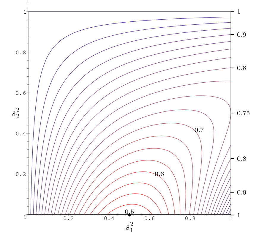
Figure 2: The ratio $N_{\mu}^{\prime}/N_{\mu}$ (it runs from $1/2$ to $1$ with contour spacing 0.025). This flux-independent quantity may be determined from the angular distribution of $\mu$-type atmospheric neutrino events.

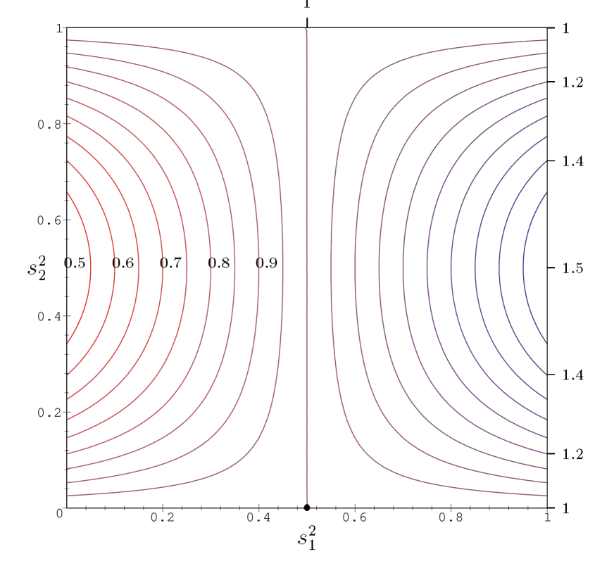
Figure 3: The ratio $N_{e}^{\prime}/N_{e}$ (it runs from $1/2$ to $3/2$ with contour spacing 0.05). This flux-independent quantity may be determined from the angular distribution of $e$-type atmospheric neutrino events.

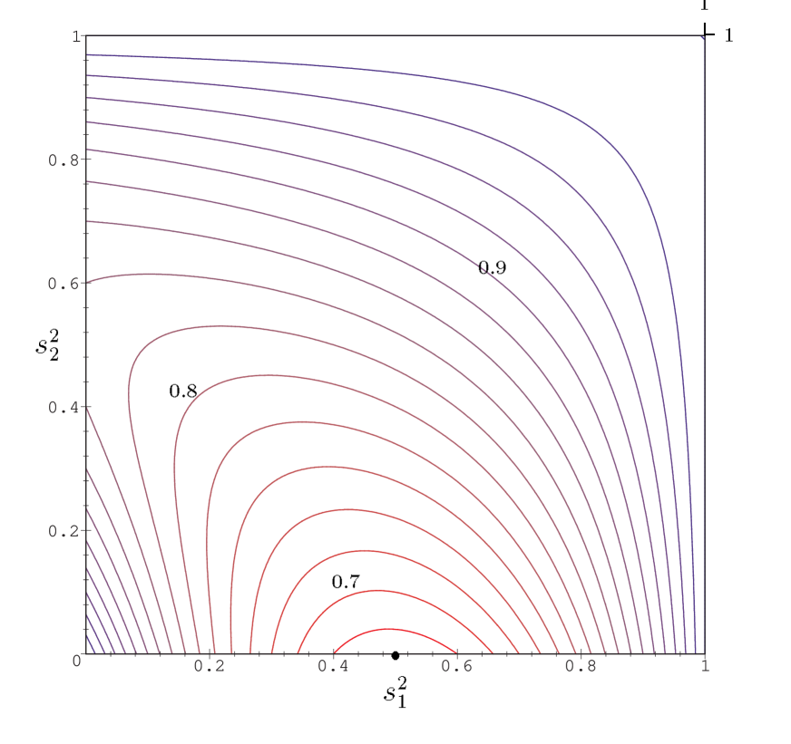
Figure 4: The overall atmospheric neutrino flux, $(N_{\mu}^{\prime}+N_{e}^{\prime})/(N_{\mu}+N_{e})$ normalized to its no-oscillation expectation (it runs from $2/3$ to $1$ with contour spacing 0.02). Current flux uncertainties prevent its precise determination.

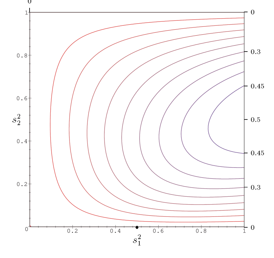
Figure 5: The flux-independent ratio $M_{e}/(M_{\mu}+M_{e})$ of $e$-like events to all events in an imagined very long baseline experiment, where $B(E)$ may be replaced by its average value of 1/2 (the ratio runs from $0$ to $1/2$ with contour spacing 0.05). In real experiments such as K2K and Minos, this replacement may not be implemented.

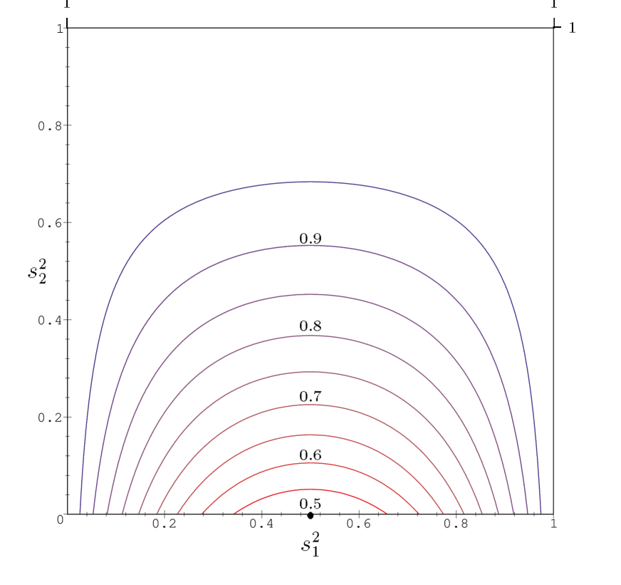
Figure 6: The ratio of the observed event rate $M_{\mu}+M_{e}$ to its value with no oscillations, again with $B=1/2$ (the ratio runs from $1/2$ to $1$ with contour spacing 0.05).

References

[1]E.g., R. Barbieri, L.J. Hall, D. Smith, A. Strumia and
N. Weiner,
“Oscillations of solar and atmospheric neutrinos,”
JHEP 12, 017 (1998)
hep-ph/9807235.
[2]
G.L. Fogli, E. Lisi, A. Marrone and G. Scioscia,
“SuperKamiokande atmospheric neutrino data, zenith distributions, and three
flavor oscillations,”
Phys. Rev. D59, 033001 (1999)
hep-ph/9808205.
[3]E.g., K. Scholberg
[SuperKamiokande Collaboration],
“Atmospheric neutrinos at SuperKamiokande,”
hep-ex/9905016, figure 4.