Abstract

The renormalization of chiral perturbation theory is carried out to next-to-next-to-leading order in the meson sector. We calculate the divergent part of the generating functional of Green functions of quark currents to $O(p^{6})$ for chiral $SU(n)$, involving one- and two-loop diagrams. The renormalization group equations for the renormalized low-energy constants of $O(p^{6})$ are derived. We compare our results with previous two-loop calculations in chiral perturbation theory.

* Work supported in part by TMR, EC-Contract No. ERBFMRX-CT980169
(EURODA$\Phi$NE).

1 Introduction

Chiral perturbation theory (CHPT) [1, 2, 3] provides a systematic low-energy expansion of QCD. In the meson sector, this expansion is now being carried out to next-to-next-to-leading order [4].

In this paper we perform the complete renormalization of the generating functional of Green functions of quark currents to $O(p^{6})$. As in every quantum field theory with a local action, the divergences of $O(p^{6})$, due to one- and two-loop diagrams, are themselves local so that the functional can be rendered finite by the chiral action of $O(p^{6})$. We carry out the calculation for chiral $SU(n)$ and then specialize to the realistic cases $n=2,3$. The divergent part of the generating functional serves as a check for existing and all future two-loop calculations in the meson sector. Moreover, the divergences govern the renormalization group equations for the renormalized low-energy constants of $O(p^{6})$. The double-pole divergences (in dimensional regularization) determine the double chiral logs, the leading infrared singularities of $O(p^{6})$ [1, 5, 6].

The main tools for this calculation are well known. One starts by expanding the chiral action around the solution of the lowest-order equation of motion (EOM) to generate the loop expansion upon functional integration. We then employ heat-kernel techniques for extracting the divergences of the generating functional. We discuss first a generic quantum field theory of scalar fields before specializing to CHPT. Special emphasis is given to certain aspects specific to nonrenormalizable quantum field theories. One subtlety concerns the dependence of the renormalization procedure on the choice of the Lagrangian of next-to-leading order, $O(p^{4})$. The allowed Lagrangians differ by EOM terms. As a consequence, the sum of one-particle-reducible (1PR) diagrams is in general divergent. It is shown that these divergences are always local and can therefore also be renormalized by the chiral action of $O(p^{6})$. Likewise, the proper renormalization at $O(p^{4})$ guarantees the absence of nonlocal subdivergences even in the presence of such EOM terms.

The major burden of this calculation is the algebraic complexity of CHPT at $O(p^{6})$. We exemplify the laborious calculations by three special cases of one-particle irreducible (1PI) diagrams. The results for $SU(n)$ and for $n=2,3$ are collected in several tables with the double-and single-pole divergences, using the standard bases of Ref. [7] for the chiral Lagrangians of $O(p^{6})$.

The paper is organized as follows. In Sec. 2, we describe the various steps of the calculation for a general scalar quantum field theory. The divergences of 1PR diagrams associated with EOM terms in the Lagrangian of next-to-leading order are shown to be local. Nonlocal subdivergences cancel, leading in particular to a set of consistency conditions for the double-pole coefficients of the 1PI diagrams [1]. In the following section, we specialize to CHPT and expand the chiral actions of $O(p^{2})$ and $O(p^{4})$ to the required orders in the fluctuation fields. Using the short-distance behaviour of (products of) Green functions [8], the determination of the divergence functional reduces to the calculation of the appropriate combinations of Seeley-DeWitt coefficients. We discuss one example each for the one-loop diagrams with a single vertex of $O(p^{4})$ and for the genuine two-loop diagrams (butterfly and sunset topologies). The renormalization procedure is described in Sec. 4 including a derivation of renormalization group equations for the renormalized low-energy constants of $O(p^{6})$. In Sec. 5, we derive the tree-level contributions of the $O(p^{6})$ Lagrangian introduced in Ref. [7] for several processes that have already been calculated to $O(p^{6})$. This allows for an immediate check of the divergence structure. Sec. 6 contains our conclusions. The singular parts of the products of operators [8] are reproduced in App. A and the manipulations for verifying the cancellation of nonlocal subdivergences are described in App. B. Our actual results in the form of double- and single-pole divergences are collected in several tables in App. C for $n=3$ and $2$ light flavours and in App. D for chiral $SU(n)$. For completeness we also give the explicit form of the terms of the $O(p^{6})$ Lagrangian in Apps. C and D.

2 Loop expansion in quantum field theory

In this section we set the general framework for our calculation. Although the treatment will be valid for any quantum field theory of scalar fields the notation is tailored to CHPT. We shall work in Euclidean space both in the present section and in the following where we describe the actual calculations. The final result in the form of the divergence functional of $O(p^{6})$ will however be given in Minkowski space in Sec. 4.

2.1 Generating functional

The starting point for a quantum field theory is the classical action $S_{2}$. We supplement this action by quantum corrections $S_{2n}$ ($n>1$) and define the total action $S$ as

$$S=S_{2}+\hbar S_{4}+\hbar^{2}S_{6}+\ldots=\sum_{n=0}^{\infty}\hbar^{n}S_{2+2n}\;\;.$$ (2.1)

The numbering of terms is chosen to comply with CHPT. Each term depends on a set of $N$ scalar fields $\phi=\{\phi_{1},\ldots,\phi_{N}\}$ and on $M$ external sources ${\bf j}=\{j_{1},\ldots,j_{M}\}$:

$$S_{i}=S_{i}[\phi,{\bf j}]\;\;.$$ (2.2)

Unlike in a renormalizable quantum field theory, the quantum corrections $S_{2n}$ ($n>1$) are in general not of the form of $S_{2}$. In fact, in CHPT the $S_{2n}$ do not have any terms in common for different $n$ because $S_{2n}$ is of chiral order $p^{2n}$.

The generating functional $Z[\bf j]$ is the logarithm of the vacuum-to-vacuum transition amplitude in the presence of the external sources. It can be defined via a path integral

$$\exp(-Z[{\bf j}]/\hbar)={\cal N}^{-1}\int\prod[d\phi_{i}]e^{-S[\phi,{\bf j}]/\hbar}$$ (2.3)

with the normalization

$$Z[0]=0\;\;.$$ (2.4)

The loop expansion can be constructed as an expansion around the solution of the classical EOM:

$$\frac{\delta S_{2}}{\delta\phi_{i}}=0\;\;\;\Rightarrow\;\;\;\phi_{\mbox{\tiny cl}}[{\bf j}]\;\;.$$ (2.5)

The action $S[\phi,{\bf j}]$ is now expanded around the classical field $\phi_{\mbox{\tiny cl}}[{\bf j}]$,

$$S[\phi,{\bf j}]=S_{2}[\phi_{\mbox{\tiny cl}},{\bf j}]+\left({1\over 2}S_{2}^{(2)}[\phi_{\mbox{\tiny cl}},{\bf j}]\xi^{2}+\hbar S_{4}[\phi_{\mbox{\tiny cl}},{\bf j}]\right)+S_{\mbox{\tiny int}}[\phi,{\bf j}]\;\;,$$ (2.6)

where $\xi_{i}=\phi_{i}-\phi_{\mbox{\tiny cl}\;i}$. Here and in the sequel we adopt the following compact notation:

$$S_{n}^{(m)}=S_{n\,i_{1},\ldots,i_{m}}^{(m)}(x_{1},\ldots,x_{m})=\frac{\delta^{m}S_{n}[\phi,{\bf j}]}{\delta\phi_{i_{1}}(x_{1})\ldots\delta\phi_{i_{m}}(x_{m})}$$ (2.7)

$$S_{n}^{(m)}\xi^{m}=\int dx_{1}\ldots dx_{m}S_{n\,i_{1},\ldots,i_{m}}^{(m)}(x_{1},\ldots,x_{m})\xi_{i_{1}}(x_{1})\ldots\xi_{i_{m}}(x_{m})\;\;.$$ (2.8)

The term $S_{2}[\phi_{\mbox{\tiny cl}},{\bf j}]$ is the only one that survives in the limit $\hbar\rightarrow 0$. In Eq. (2.6) we have written between parentheses the terms that after functional integration contribute to $O(\hbar)$. The rest is denoted $S_{\mbox{\tiny int}}[\phi,{\bf j}]$. Restricted to terms contributing to $O(\hbar^{2})$, it takes the explicit form

$$S_{\mbox{\tiny int}}[\phi,{\bf j}] = {1\over 3!}S_{2}^{(3)}[\phi_{\mbox{\tiny cl}},{\bf j}]\xi^{3}+{1\over 4!}S_{2}^{(4)}[\phi_{\mbox{\tiny cl}},{\bf j}]\xi^{4}+\ldots$$ (2.9)

$$+ \hbar\left(S_{4}^{(1)}[\phi_{\mbox{\tiny cl}},{\bf j}]\xi+{1\over 2}S_{4}^{(2)}[\phi_{\mbox{\tiny cl}},{\bf j}]\xi^{2}+\ldots\right)$$

$$+ \hbar^{2}S_{6}[\phi_{\mbox{\tiny cl}},{\bf j}]\;\;.$$

Functional integration over the fluctuation fields $\xi_{i}$ in (2.3) gives rise to an expansion of the generating functional $Z[\bf j]$ in powers of $\hbar$,

$$Z=Z_{0}+\hbar Z_{1}+\hbar^{2}Z_{2}+O(\hbar^{3})\;\;,$$ (2.10)

where

$$Z_{0} = \overline{S_{2}}\;\;,$$

$$Z_{1} = \overline{S_{4}}+\frac{1}{2}\mbox{Tr}\ln\left({\Delta\over\Delta_{0}}\right)\;\;$$

$$Z_{2} = \overline{S_{6}}+z_{2}\;\;.$$ (2.11)

$\overline{S_{n}}=S_{n}[\phi_{\mbox{\tiny cl}},{\bf j}]$ is the action evaluated at the classical field and $\Delta=S_{2}^{(2)}[\phi_{\mbox{\tiny cl}},{\bf j}]$ is a differential operator. The subscript $0$ in $\Delta_{0}$ indicates that the operator is to be evaluated for ${\bf j}=0$.

The explicit expression for $z_{2}$ is

$$z_{2} = {1\over 8}S_{2\;ijkl}^{(4)}G_{ij}G_{kl}-{1\over 12}S_{2\;ijk}^{(3)}G_{ir}G_{js}G_{kt}S_{2\;rst}^{(3)}-{1\over 8}S_{2\;ijk}^{(3)}G_{ij}G_{kt}G_{rs}S_{2\;rst}^{(3)}$$ (2.12)

$$+ {1\over 2}S_{4\;ij}^{(2)}G_{ij}-{1\over 2}S_{2\;ijk}^{(3)}G_{jk}G_{il}S_{4\;l}^{(1)}$$

$$- {1\over 2}S_{4\;i}^{(1)}G_{ij}S_{4\;j}^{(1)}\;\;,$$

where $G_{ij}$ is the inverse of the differential operator $\Delta$:

$$\Delta_{ij}(x)G_{jk}(x,y)=\delta_{ik}\delta^{(4)}(x-y)\;\;.$$ (2.13)

Summation over repeated indices is understood. In Eq. (2.12) we have adopted a compact notation where the Latin indices stand both for flavour (discrete) and space-time (continuous) indices. Repeated Latin indices indicate both a summation over flavour indices and integration over space-time variables.

The terms in Eq. (2.12) include two-loop (first line), one-loop (second line) and tree-level contributions (third line, together with $\overline{S_{6}}$ in (2.11)). In the order written, they correspond to the diagrams shown in Fig. 1.

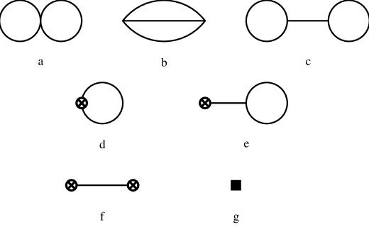
Figure 1: Diagrams contributing to the generating functional $Z_{2}$ in (2.11). The propagators and vertices carry the full tree structure associated with the lowest-order action $S_{2}$. Normal vertices are from $S_{2}$, crossed circles denote vertices from $S_{4}$. The diagrams are shown in the order appearing in (2.12). Diagram g denotes tree diagrams corresponding to $\overline{S_{6}}$ in (2.11).

2.2 Heat-kernel expansion

To calculate the divergent part of the generating functional we use the well-known heat-kernel technique. We sketch here the procedure and introduce the relevant notation, following closely the presentation of Ref. [8].

Given an elliptic differential operator $\Delta$,

$$\Delta(x)=-d_{x}^{2}+\sigma(x)\;,\;\;\;d_{\mu}=\partial_{\mu}+\gamma_{\mu}(x)\;\;,$$ (2.14)

where both $\sigma$ and $\gamma_{\mu}$ are matrices in general, we define its heat kernel as the function that satisfies the heat diffusion equation

$$\left({\partial\over\partial t}+\Delta(x)\right){\cal G}_{\Delta}(x,y;t)=0$$ (2.15)

with the boundary condition

$${\cal G}_{\Delta}(x,y;0)=\delta^{d}(x-y)\;\;.$$ (2.16)

The Green function of the operator $\Delta$ is then given by

$$G_{\Delta}(x,y) = \int_{0}^{\infty}{\cal G}_{\Delta}(x,y;t)\,dt$$

$$\Delta(x)G_{\Delta}(x,y) = \delta^{d}(x-y)\;\;.$$ (2.17)

The singularities responsible for the divergences of the generating functional arise from the short-distance behaviour ($y\rightarrow x$) of the Green function $G_{\Delta}(x,y)$. To extract these singularities, we can use the asymptotic expansion of the heat kernel for $t\rightarrow 0_{+}$:

$${\cal G}_{\Delta}(x,y;t)=\frac{1}{(4\pi t)^{d/2}}e^{-{|x-y|^{2}\over 4t}}\sum_{n=0}^{\infty}a_{n}^{\Delta}(x,y)t^{n}\;\;.$$ (2.18)

The first Seeley-DeWitt coefficients are (in the coincidence limit $y\rightarrow x$)

$$a_{0}^{\Delta}(x,x) = 1$$

$$a_{1}^{\Delta}(x,x) = -\sigma(x)$$

$$a_{2}^{\Delta}(x,x) = {1\over 12}\gamma_{\mu\nu}(x)\gamma_{\mu\nu}(x)+{1\over 2}\sigma^{2}(x)-{1\over 6}d^{2}\sigma(x)$$ (2.19)

where $\gamma_{\mu\nu}$ is the usual field strength associated with $\gamma_{\mu}$.

Correspondingly, we can write the Green function $G_{\Delta}$ as

$$G_{\Delta}(x,y) = G_{0}(x-y)a_{0}^{\Delta}(x,y)+R_{1}(x-y;c\mu)a_{1}^{\Delta}(x,y)$$ (2.20)

$$+ R_{2}(x-y;c\mu)a_{2}^{\Delta}(x,y)+\overline{G}_{\Delta}(x,y;c\mu)\;\;.$$

The various functions in (2.20) are defined by [8]

$$G_{0}(x) = \frac{\Gamma(d/2-1)}{4\pi^{d/2}}|x|^{2-d}$$

$$R_{1}(x;c\mu) = \frac{1}{16\pi^{2}}\left[{-2(c\mu)^{d-4}\over d-4}+\frac{\Gamma(d/2-2)}{\pi^{d/2-2}}|x|^{4-d}\right]$$

$$R_{2}(x;c\mu) = \frac{|x|^{2}}{32\pi^{2}}\left[{(c\mu)^{d-4}\over d-4}+\frac{\Gamma(d/2-3)}{2\pi^{d/2-2}}|x|^{4-d}\right]\;\;.$$ (2.21)

We have regularized the short-distance singularities by dimensional regularization. The scale-dependent coefficient functions $R_{1}$ and $R_{2}$ are defined such that they are regular for $d\rightarrow 4$. The positive constant $c$ parametrizes different regularization conventions ($c=1$ for minimal subtraction). We shall follow the usual convention of CHPT [2, 3] with

$$\ln c=-\frac{1}{2}\left[\ln 4\pi+\Gamma^{\prime}(1)+1\right]$$ (2.22)

and employ the notation

$$\Lambda=\frac{1}{16\pi^{2}(d-4)}\;\;.$$ (2.23)

By construction, $\overline{G}_{\Delta}(x,y;c\mu)$ has no poles in $d-4$ and is regular for $x\rightarrow y$, $d\to 4$ even for two derivatives. It is scale and convention dependent compensating the corresponding dependences of $R_{1}$, $R_{2}$.

With these definitions, one obtains [8] the propagator and its derivatives in the coincidence limit $x\rightarrow y$ by analytic continuation in $d$:

$$G_{\Delta}(x,x) = -2(c\mu)^{d-4}\Lambda\,a_{1}^{\Delta}(x,x)+\overline{G}_{\Delta}(x,x;c\mu)$$

$$d_{\mu}^{x}G_{\Delta}(x,y)_{|_{y=x}} = -2(c\mu)^{d-4}\Lambda\,d^{x}_{\mu}a_{1}^{\Delta}(x,y)_{|_{y=x}}+d^{x}_{\mu}\overline{G}_{\Delta}(x,y;c\mu)_{|_{y=x}}$$

$$d_{\mu}^{x}d_{\nu}^{y}G_{\Delta}(x,y)_{|_{y=x}} = -2(c\mu)^{d-4}\Lambda\left(d^{x}_{\mu}d^{y}_{\nu}a_{1}^{\Delta}(x,y)_{|_{y=x}}+{\delta_{\mu\nu}\over 2}a_{2}^{\Delta}(x,x)\right)$$ (2.24)

$$+d^{x}_{\mu}d^{y}_{\nu}\overline{G}_{\Delta}(x,y;c\mu)_{|_{y=x}}\;\;$$

where

$$d_{\mu}^{y}G_{\Delta}(x,y)=\partial_{\mu}^{y}G_{\Delta}(x,y)-G_{\Delta}(x,y)\gamma_{\mu}(y)~{}.$$ (2.25)

The one-loop singularities can also be obtained from the heat-kernel representation as

$$\mbox{Tr}\ln\left(\frac{\Delta}{\Delta_{0}}\right)=-\int_{0}^{\infty}\frac{dt}{t}\int d^{d}x\left[{\cal G}_{\Delta}(x,x;t)-{\cal G}_{\Delta_{0}}(x,x;t)\right]\;\;,$$ (2.26)

leading to the well-known result

$$\mbox{Tr}\ln\left(\frac{\Delta}{\Delta_{0}}\right)=2(c\mu)^{d-4}\Lambda\int d^{d}x\,\mbox{tr}\left[a_{2}^{\Delta}(x,x)-a_{2}^{\Delta_{0}}(x,x)\right]+\mbox{finite terms}\;\;.$$ (2.27)

At the two-loop level the singularities come from the short-distance behaviour of products of two or three propagators and derivatives thereof (cf. Eq. (2.12)). To extract these singularities, one uses the representation (2.20) and analyses products of the three functions $G_{0}$, $R_{1}$, $R_{2}$ and their derivatives at short distances. As an example,

$$G_{0}(x)^{2}\sim-\frac{1}{8\pi^{2}(d-4)}\delta^{d}(x)\;\;.$$ (2.28)

All products relevant for our calculation were calculated first in Ref. [8]. We have checked their results and for convenience we reproduce them in App. A. Each of the terms in Eq. (2.12) has both local and nonlocal singularities. To be able to renormalize the theory, the latter have to cancel in the sum. In the following three subsections we will prove that this is indeed the case. We first consider the 1PR diagrams which have nonlocal singularities of the form $A(x)G(x,y)B(y)$, and then the nonlocal subdivergences in the 1PI diagrams. In the last subsection we will single out the divergences of the form $1/(d-4)\times\ln m^{2}$ which appear in all 1PI diagrams. The requirement that they cancel leads to a nontrivial relation between the coefficients of the double poles of the 1PI two-loop diagrams (a and b in Fig. 1) and the double poles of the 1PI one-loop diagram (d in Fig. 1).

2.3 One-particle-reducible diagrams

The three 1PR diagrams (c,e,f in Fig. 1) are individually divergent and these divergences are in general nonlocal. In a consistent quantum field theory, these nonlocal divergences have to cancel. Only local divergences (polynomials in masses and derivatives) are allowed because it would otherwise be impossible to render the theory finite by adding the local action $S_{6}$.

The proof for this cancellation of nonlocal divergences runs as follows. We can write the sum of the three 1PR diagrams as

$$Z_{2}^{\mbox{\tiny 1PR}}=-{1\over 2}\left[S^{(1)}_{4\;i}+{1\over 2}S^{(3)}_{2\;ijk}G_{jk}\right]G_{il}\left[S^{(1)}_{4\;l}+{1\over 2}S^{(3)}_{2\;lrs}G_{rs}\right]\;\;.$$ (2.29)

Recall that all quantities are to be taken at the classical field $\phi_{\mbox{\tiny cl}}[{\bf j}]$. The terms inside the square brackets are nothing but the derivative of the $O(\hbar)$ term of the generating functional, $Z_{1}$, which is finite by construction:

$$S^{(1)}_{4\;i}+{1\over 2}S^{(3)}_{2\;ijk}G_{jk}={\delta Z_{1}\over\delta\phi_{i}}\;\;.$$ (2.30)

Since $Z_{1}$ is finite this would seem to prove that also $Z_{2}^{\mbox{\tiny 1PR}}$ in (2.29) is finite. The problem is that the procedures of functional derivation and setting $\phi=\phi_{\mbox{\tiny cl}}[{\bf j}]$ do not commute in general because $S_{4}$ may contain (divergent) terms that vanish at the classical field. Denoting such terms as $S_{4}^{\mbox{\tiny EOM}}$, we may therefore have

$$S_{4}^{\mbox{\tiny EOM}}[\phi_{\mbox{\tiny cl}}]=0,\;\;\;\;\;\;\left({\delta S_{4}^{\mbox{\tiny EOM}}[\phi]\over\delta\phi_{i}}\right)_{|_{\phi=\phi_{\mbox{\tiny cl}}}}\neq 0\;\;,$$ (2.31)

making $Z_{2}^{\mbox{\tiny 1PR}}$ divergent in general. Such terms must be of the form

$$S_{4}^{\mbox{\tiny EOM}}=\,\Xi\,X_{i}[\phi]{\delta S_{2}\over\delta\phi_{i}}$$ (2.32)

where $\,\Xi\,$ is a coupling constant that may be divergent for $d\to 4$. Taking the functional derivative and setting $\phi=\phi_{\mbox{\tiny cl}}$, we obtain

$$\left({\delta S_{4}^{\mbox{\tiny EOM}}[\phi]\over\delta\phi_{j}}\right)_{|_{\phi=\phi_{\mbox{\tiny cl}}}}=\,\Xi\,X_{i}[\phi_{\mbox{\tiny cl}}]S^{(2)}_{2\;ij}=\,\Xi\,X_{i}[\phi_{\mbox{\tiny cl}}]\Delta_{ij}\;\;.$$ (2.33)

Therefore, the contribution of such terms to the 1PR diagrams is

$$-{1\over 2}\,\Xi^{2}\,X_{i}\Delta_{ij}X_{j}-\,\Xi\,X_{i}{\delta Z^{0}_{1}\over\delta\phi_{i}}\;\;.$$ (2.34)

Here, $Z^{0}_{1}$ is by definition free from terms that vanish at the classical field and its derivative is therefore finite. The first term in Eq. (2.34) is divergent (when $\Xi$ is divergent) but has the form of a local action, which is perfectly allowed. On the other hand, the second term is also divergent but contains a nonlocal piece

$$-{1\over 2}\,\Xi\,X_{i}S_{2\;ijk}^{(3)}\overline{G}_{jk}\;\;.$$ (2.35)

Such a nonlocal divergence must not be present in the final result. In fact, it is rather easy to see that it is cancelled by the 1PI contribution of $S_{4}^{\mbox{\tiny EOM}}$ (diagram d in Fig. 1):

$${1\over 2}\left({\delta^{2}S_{4}^{\mbox{\tiny EOM}}\over\delta\phi_{j}\delta\phi_{k}}\right)_{|_{\phi=\phi_{\mbox{\tiny cl}}}}G_{jk} = {1\over 2}\,\Xi\,\left[{\delta X_{i}\over\delta\phi_{k}}\Delta_{ij}+X_{i}S^{(3)}_{2\;ijk}\right]G_{jk}$$ (2.36)

$$= {1\over 2}\,\Xi\,{\delta X_{i}\over\delta\phi_{i}}+{1\over 2}\,\Xi\,X_{i}S^{(3)}_{2\;ijk}G_{jk}\;\;.$$

The sum of (2.34) and (2.36) is in general divergent but it has the form of a local action that can be renormalized by $S_{6}$.

2.4 Absence of nonlocal subdivergences

The three 1PI graphs (diagrams a,b,d in Fig. 1) are the source of the “true” divergences of $O(\hbar^{2})$. However, part of the divergences occurring in the individual graphs have to cancel in the sum. These are the so-called “nonlocal subdivergences” due to one-loop subgraphs. As is well known, these nonlocal subdivergences cancel if the renormalization was properly done at $O(\hbar)$. Of course, we will verify this explicitly in our calculation (see also Ref. [6]). Here we present a general proof within our formalism.

Let us start from the definition of the 1PI part of the generating functional of $O(\hbar^{2})$:

$$Z_{2}^{\mbox{\tiny 1PI}}={1\over 8}S_{2\;ijkl}^{(4)}G_{ij}G_{kl}-{1\over 12}S_{2\;ijk}^{(3)}G_{ir}G_{js}G_{kt}S_{2\;rst}^{(3)}+{1\over 2}S_{4\;ij}^{(2)}G_{ij}\;\;.$$ (2.37)

The problematic divergences arise when one of the propagators in each term in (2.37) is replaced by its finite part $\overline{G}$:

$$Z_{2}^{\mbox{\tiny subdiv}}=\left[{1\over 4}S_{2\;ijkl}^{(4)}G_{ij}-{1\over 4}S_{2\;ijk}^{(3)}G_{ir}G_{js}S_{2\;rsl}^{(3)}+{1\over 2}S_{4\;kl}^{(2)}\right]\overline{G}_{kl}\;\;.$$ (2.38)

As in the previous subsection, the key observation is that the term between square brackets is proportional to the double functional derivative of $Z_{1}$, the $O(\hbar)$ term in the generating functional, and is therefore finite. Again this argument has a similar loophole as before connected with the possible presence of divergent terms that vanish at the classical field. Because of such terms the finiteness of $Z_{1}$ (evaluated at the classical field) does not imply that its double functional derivative is also finite. However, we have already seen that the nonlocal subdivergences generated by such terms in the 1PI graphs are compensated exactly by similar terms in the 1PR part. This concludes the proof that nonlocal subdivergences cancel at $O(\hbar^{2})$.

2.5 Weinberg consistency conditions

The fact that the residues of the poles in $d-4$ have to be polynomials in external momenta and masses [9] implies nontrivial relations between the coefficients of the divergences of the three 1PI diagrams. To derive this consequence, we have to look at the terms depending logarithmically on the masses that appear in the residues of the single poles. Diagrams a and b have the following structure:

$$\mbox{`a+b'}=\int\!\!d^{d}x\mu^{2(d-4)}\left[\Lambda^{2}\sum_{a}\alpha_{a}Y_{a}(x)+{\Lambda\over 16\pi^{2}}\left(\sum_{a}\beta_{a}Y_{a}(x)+M(x)\right)+{N(x)\over(16\pi^{2})^{2}}\right]\;\;,$$ (2.39)

where the $Y_{a}(x)$ are a complete set of local operators appearing in the action $S_{6}$, and $M(x)$, $N(x)$ are two generic functions which contain the nonlocal terms generated by the loop integrals. By definition, $M(x)$ does not contain any local terms that can be expressed as linear combinations of the $Y_{a}(x)$. The overall coefficient $\mu^{2(d-4)}$ ensures the correct dimensions but is completely arbitrary, as in both diagrams the scale $\mu$ does not appear at all. In fact, Eq. (2.39) is $\mu$-independent by definition, which implies the following equations:

$$\mu{\partial\alpha_{a}\over\partial\mu} = 0$$

$$\mu{\partial\beta_{a}\over\partial\mu} = -2\alpha_{a}$$ (2.40)

$$\mu{\partial M(x)\over\partial\mu} = 0$$

$$\mu{\partial N(x)\over\partial\mu} = -2\left(\sum_{a}\beta_{a}Y_{a}(x)+M(x)\right)\;\;.$$

From Eq. (2.40) it is clear that the residue of the single pole in $d-4$ contains terms of the form $\ln m^{2}/\mu^{2}$, where $m$ is one of the masses of the particles in the theory. Such terms can only be cancelled by analogous ones in the one-loop diagram d. The latter is of the form

$$\mbox{`d'}=\int\!\!d^{d}x\sum_{i}\hat{L}_{i}\mu^{d-4}\left(\Lambda\sum_{a}\eta_{a}^{i}Y_{a}(x)+{1\over 16\pi^{2}}H_{i}(x)\right)\;\;,$$ (2.41)

where the $\hat{L}_{i}$ are the coefficients in front of the operators $X_{i}$ appearing in the action $S_{4}$: $S_{4}=\int d^{d}x\sum_{i}\hat{L}_{i}X_{i}$. $H_{i}(x)$ are generic functions containing the nonlocal part of the loop integrals. For each $i$, the one-loop diagram is again $\mu$-independent. Since all the $\hat{L}_{i}$ are themselves $\mu$-independent by definition we obtain

$$\mu{\partial\eta_{a}^{i}\over\partial\mu} = 0$$

$$\mu{\partial H_{i}(x)\over\partial\mu} = -\sum_{a}\eta_{a}^{i}Y_{a}(x)\;\;.$$ (2.42)

The $\hat{L}_{i}$ are in general divergent,

$$\hat{L}_{i}=\mu^{d-4}\left({\hat{\Gamma}}_{i}\Lambda+\hat{L}_{i}^{r}(\mu,d)\right)\;\;,$$ (2.43)

and therefore also the one-loop diagram has logarithms of the masses in the residue of the single pole. The condition that these logarithms cancel in the sum implies the following relations [1]:

$$\alpha_{a}=-{1\over 2}\sum_{i}{\hat{\Gamma}}_{i}\eta_{a}^{i}~{}.$$ (2.44)

The cancellation of the other nonlocal terms requires

$$M(x)=-\sum_{i}{\hat{\Gamma}}_{i}\bar{H}_{i}(x)\;\;,$$ (2.45)

where

$$\bar{H}_{i}(x)=H_{i}(x)-{1\over 2}\ln{m^{2}\over\mu^{2}}\sum_{a}\eta^{i}_{a}Y_{a}(x)\;\;.$$ (2.46)

3 Chiral perturbation theory to two loops

Having set up the general framework, we now specialize to CHPT. As we will see, the divergence calculation is now only a matter of (long and tedious) algebraic manipulations. The procedure, on the other hand, is well defined and completely straightforward. It amounts to the following steps:

1. Define the first three terms in the action: $S_{2}$, $S_{4}$ and $S_{6}$;

2. Define the differential operator $\Delta$ for CHPT and calculate the corresponding Seeley-DeWitt coefficients;

3. Expand $S_{2}$ ($S_{4}$) up to fourth (second) order in $\xi$;

4. Contract indices between the vertices $S_{2n\,i_{1},\ldots i_{m}}^{(m)}$ and the Seeley-DeWitt coefficients appropriately;

5. Finally, reduce everything to the standard basis defined by $S_{6}$.

In the following we will give all the necessary ingredients for this lengthy calculation. In the next section, we present our final results for chiral $SU(n)$ and for the physically relevant cases $n=2,3$.

3.1 Preliminaries

In Euclidean space, the $O(p^{2})$ Lagrangian is given by [2, 3]

$${\cal L}_{2}={F^{2}\over 4}\langle u_{\mu}u_{\mu}-\chi_{+}\rangle$$ (3.1)

with

$$u_{\mu} = i\{u^{\dagger}(\partial_{\mu}-ir_{\mu})u-u(\partial_{\mu}-i\ell_{\mu})u^{\dagger}\}$$

$$\chi_{\pm} = u^{\dagger}\chi u^{\dagger}\pm u\chi^{\dagger}u\,.$$ (3.2)

Here, $u(\phi)$ is the usual matrix field of Goldstone bosons and the external fields $v_{\mu},a_{\mu},s,p$ are contained in $r_{\mu}=v_{\mu}+a_{\mu}$, $\ell_{\mu}=v_{\mu}-a_{\mu}$, $\chi=2B(s+ip)$. The symbol $\langle\dots\rangle$ denotes the $n$-dimensional flavour trace for chiral $SU(n)$ and $F,B$ are the two low-energy constants of $O(p^{2})$. The EOM (2.5) take the form

$$\nabla_{\mu}u_{\mu}+{i\over 2}\hat{\chi}_{-}=0$$ (3.3)

with

$$\nabla_{\mu}X = \partial_{\mu}X+[\Gamma_{\mu},X]$$

$$\Gamma_{\mu} = {1\over 2}\left[u^{\dagger}(\partial_{\mu}-ir_{\mu})u+u(\partial_{\mu}-il_{\mu})u^{\dagger}\right]$$

$$\hat{\chi}_{-} = \chi_{-}-1/n\langle\chi_{-}\rangle~{}.$$ (3.4)

Expanding ${\cal L}_{2}$ around the classical field, the solution of the EOM (3.3), we obtain the $(n^{2}-1)$-dimensional matrix-differential operator $\Delta$:

$$\Delta=-d_{\mu}d_{\mu}+\sigma\;\;,$$ (3.5)

where

$$d_{\mu} = \partial_{\mu}+\gamma_{\mu}$$

$$\gamma_{\mu\,ab} = -{1\over 2}\langle\Gamma_{\mu}[\lambda_{a},\lambda_{b}]\rangle$$

$$\sigma_{ab} = {1\over 8}\langle[u_{\mu},\lambda_{a}][u_{\mu},\lambda_{b}]+\left\{\lambda_{a},\lambda_{b}\right\}\chi_{+}\rangle\;\;.$$ (3.6)

We use the normalization $\langle\lambda_{a}\lambda_{b}\rangle=2\delta_{ab}$ and we define the fluctuation fields $\xi$ via

$$u^{2}(\phi)=u(\phi_{\mbox{\tiny cl}})e^{\frac{i\sqrt{2}}{F}\xi}u(\phi_{\mbox{\tiny cl}})~{}.$$ (3.7)

In the notation of the previous section, the third- and fourth-order terms in the expansion around the classical field are given by:

$$S_{2}^{(3)}\xi^{3} = -{\sqrt{2}\over F}\int d^{d}x\left[3\langle\xi\nabla_{\mu}\xi\xi u_{\mu}\rangle+{i\over 2n}\langle\chi_{-}\rangle\langle\xi^{3}\rangle\right]$$ (3.8)

$$S_{2}^{(4)}\xi^{4} = {2\over F^{2}}\int d^{d}x\langle[\xi,\nabla_{\mu}\xi][\xi,\nabla_{\mu}\xi]+{1\over 4}\left[\xi,[u_{\mu},\xi]\right]^{2}-{1\over 2}\chi_{+}\xi^{4}\rangle\;\;.$$ (3.9)

The most general chiral $SU(n)$ Lagrangian of $O(p^{4})$ is given by

$${\cal L}_{4} = \sum_{i=0}^{12}{\hat{L}}_{i}X_{i}+\mbox{contact terms}$$ (3.10)

$$= -{\hat{L}}_{0}\langle u_{\mu}u_{\nu}u_{\mu}u_{\nu}\rangle-{\hat{L}}_{1}\langle u\hskip-1.29167pt\cdot\hskip-1.29167ptu\rangle^{2}-{\hat{L}}_{2}\langle u_{\mu}u_{\nu}\rangle\langle u_{\mu}u_{\nu}\rangle-{\hat{L}}_{3}\langle(u\hskip-1.29167pt\cdot\hskip-1.29167ptu)^{2}\rangle$$

$$+ {\hat{L}}_{4}\langle u\hskip-1.29167pt\cdot\hskip-1.29167ptu\rangle\langle\chi_{+}\rangle+{\hat{L}}_{5}\langle u\hskip-1.29167pt\cdot\hskip-1.29167ptu\chi_{+}\rangle-{\hat{L}}_{6}\langle\chi_{+}\rangle^{2}-{\hat{L}}_{7}\langle\chi_{-}\rangle^{2}$$

$$- {{\hat{L}}_{8}\over 2}\langle\chi_{+}^{2}+\chi_{-}^{2}\rangle+i{\hat{L}}_{9}\langle f_{+\,\mu\nu}u_{\mu}u_{\nu}\rangle-{{\hat{L}}_{10}\over 4}\langle f_{+}^{2}-f_{-}^{2}\rangle$$

$$+ i{\hat{L}}_{11}\langle\hat{\chi}_{-}(\nabla_{\mu}u_{\mu}+{i\over 2}\hat{\chi}_{-})\rangle-{\hat{L}}_{12}\langle(\nabla_{\mu}u_{\mu}+{i\over 2}\hat{\chi}_{-})^{2}\rangle$$

$$+ \mbox{contact terms}\;\;,$$

where $u\hskip-1.29167pt\cdot\hskip-1.29167ptu=u_{\mu}u_{\mu}$, $f_{\pm}^{2}=f_{\pm\,\mu\nu}f_{\pm\;\mu\nu}$ and

$$f_{\pm\;\mu\nu} = uF_{L\;\mu\nu}u^{\dagger}\pm u^{\dagger}F_{R\;\mu\nu}u$$

$$F_{R\;\mu\nu} = \partial_{\mu}r_{\nu}-\partial_{\nu}r_{\mu}-i[r_{\mu},r_{\nu}]$$

$$F_{L\;\mu\nu} = \partial_{\mu}\ell_{\nu}-\partial_{\nu}\ell_{\mu}-i[\ell_{\mu},\ell_{\nu}]~{}.$$ (3.11)

The renormalization at the one-loop level is performed by splitting the constants ${\hat{L}}_{i}$ into a divergent and a finite part:

$${\hat{L}}_{i}=(c\mu)^{d-4}\left[{\hat{\Gamma}}_{i}\Lambda+{\hat{L}}_{i}^{r}(\mu,d)\right]\;\;,$$ (3.12)

where $c$ and $\Lambda$ are defined in Eqs. (2.22), (2.23). The measurable low-energy constants ${\hat{L}}_{i}^{r}(\mu)$ (or rather the corresponding constants for $n=2$ or $3$) are given by

$${\hat{L}}_{i}^{r}(\mu)={\hat{L}}_{i}^{r}(\mu,4)~{}.$$ (3.13)

The expressions for the coefficients ${\hat{\Gamma}}_{i}$ can be obtained from Eq. (2.27) by taking the trace of the Seeley-DeWitt coefficient $a_{2}(x,x)$ in CHPT [3]:

$${\hat{\Gamma}}_{0}={n\over 48}\;, {\hat{\Gamma}}_{1}={1\over 16}\;,\qquad{\hat{\Gamma}}_{2}={1\over 8}\;,$$

$${\hat{\Gamma}}_{3}={n\over 24}\;, {\hat{\Gamma}}_{4}={1\over 8}\;,\qquad{\hat{\Gamma}}_{5}={n\over 8}\;,$$

$${\hat{\Gamma}}_{6}={n^{2}+2\over 16n^{2}}\;, {\hat{\Gamma}}_{7}=0\;,\qquad{\hat{\Gamma}}_{8}={n^{2}-4\over 16n}\;,$$

$${\hat{\Gamma}}_{9}={n\over 12}\;, {\hat{\Gamma}}_{10}=-{n\over 12}\;\;.$$ (3.14)

For $n=2,3$, not all the monomials in the Lagrangian (3.10) are linearly independent. The $SU(3)$ Lagrangian of Ref. [3] is recovered with the help of the relations

$$L_{1}={\hat{L}}_{0}/2+{\hat{L}}_{1}\;,\qquad L_{2}={\hat{L}}_{0}+{\hat{L}}_{2}\;,\qquad L_{3}=-2{\hat{L}}_{0}+{\hat{L}}_{3}$$

$$L_{i}={\hat{L}}_{i}\;(i=4,\ldots,10)\;,\qquad{\hat{L}}_{11}={\hat{L}}_{12}=0\;.$$ (3.15)

The corresponding relations for the $SU(2)$ Lagrangian of Ref. [2] are

$$l_{1}=-2{\hat{L}}_{0}+4{\hat{L}}_{1}+2{\hat{L}}_{3}\;,\qquad l_{2}=4({\hat{L}}_{0}+{\hat{L}}_{2})$$

$$l_{3}=4(-2{\hat{L}}_{4}-{\hat{L}}_{5}+4{\hat{L}}_{6}+2{\hat{L}}_{8})\;,\qquad l_{4}=4(2{\hat{L}}_{4}+{\hat{L}}_{5})$$

$$l_{5}={\hat{L}}_{10}\;,\quad l_{6}=-2{\hat{L}}_{9}\;,\quad l_{7}=-8(2{\hat{L}}_{7}+{\hat{L}}_{8})$$

$${\hat{L}}_{11}=-l_{4}/4\;,\qquad{\hat{L}}_{12}=0~{}.$$ (3.16)

Note that there is an EOM term of the type (2.32) proportional to $l_{4}$ in the two-flavour case.

3.2 One-loop diagram

To calculate the divergences arising from the one-loop diagram with ${\cal L}_{4}$ (diagram d in Fig. 1), we first need to expand the thirteen terms in the Lagrangian (3.10) in the fluctuation fields $\xi$ according to

$$X_{i}=X^{(0)}_{i}+X_{i}^{(1)}\xi+{1\over 2}X_{i}^{(2)}\xi^{2}+O(\xi^{3})\,,$$ (3.17)

where the coefficients $X^{(0)}_{i}$, $X_{i}^{(1)}$ and $X_{i}^{(2)}$ are to be taken at the classical field. Their explicit expressions are as follows:

$$X_{0} = X^{(0)}_{0}+\frac{4\sqrt{2}}{F}\langle\nabla_{\mu}\xi u_{\nu}u_{\mu}u_{\nu}\rangle-\frac{1}{F^{2}}\left(8\langle\nabla_{\mu}\xi\nabla_{\nu}\xi u_{\mu}u_{\nu}\rangle+4\langle\nabla_{\mu}\xi u_{\nu}\nabla_{\mu}\xi u_{\nu}\rangle\right.$$

$$\left.+\langle u_{\mu}u_{\nu}u_{\mu}\left[\xi,\left[u_{\nu},\xi\right]\right]\rangle\right)+O(\xi^{3})$$

$$X_{1} = X^{(0)}_{1}+\frac{4\sqrt{2}}{F}\langle u\hskip-1.29167pt\cdot\hskip-1.29167ptu\rangle\langle\nabla_{\nu}\xi u_{\nu}\rangle-\frac{8}{F^{2}}\langle\nabla_{\mu}\xi u_{\mu}\rangle\langle\nabla_{\nu}\xi u_{\nu}\rangle$$

$$-\frac{4}{F^{2}}\langle u\hskip-1.29167pt\cdot\hskip-1.29167ptu\rangle\left(\langle\nabla_{\nu}\xi\nabla_{\nu}\xi\rangle+{1\over 4}\langle\left[u_{\nu},\xi\right]\left[u_{\nu},\xi\right]\rangle\right)+O(\xi^{3})$$

$$X_{2} = X^{(0)}_{2}+\frac{4\sqrt{2}}{F}\langle u_{\mu}u_{\nu}\rangle\langle u_{\mu}\nabla_{\nu}\xi\rangle-\frac{4}{F^{2}}\langle u_{\mu}\nabla_{\nu}\xi\rangle\langle u_{\mu}\nabla_{\nu}\xi+u_{\nu}\nabla_{\mu}\xi\rangle$$

$$-\frac{4}{F^{2}}\langle u_{\mu}u_{\nu}\rangle\left(\langle\nabla_{\mu}\xi\nabla_{\nu}\xi\rangle+{1\over 4}\langle\left[u_{\mu},\xi\right]\left[u_{\nu},\xi\right]\rangle\right)+O(\xi^{3})$$

$$X_{3} = X^{(0)}_{3}+\frac{2\sqrt{2}}{F}\langle u\hskip-1.29167pt\cdot\hskip-1.29167ptu\left\{u_{\nu},\nabla_{\nu}\xi\right\}\rangle-\frac{1}{F^{2}}\left(2\langle\left\{u_{\mu},\nabla_{\mu}\xi\right\}\left\{u_{\nu},\nabla_{\nu}\xi\right\}\rangle\right.$$

$$\left.+4\langle u\hskip-1.29167pt\cdot\hskip-1.29167ptu\nabla_{\nu}\xi\nabla_{\nu}\xi\rangle+\langle\left\{u\hskip-1.29167pt\cdot\hskip-1.29167ptu,u_{\nu}\right\}\xi\left[u_{\nu},\xi\right]\rangle\right)+O(\xi^{3})$$

$$X_{4} = X^{(0)}_{4}-\frac{2\sqrt{2}}{F}\langle u_{\mu}\nabla_{\mu}\xi\rangle\langle\chi_{+}\rangle-\frac{i\sqrt{2}}{F}\langle u\hskip-1.29167pt\cdot\hskip-1.29167ptu\rangle\langle\xi\chi_{-}\rangle$$

$$-\frac{1}{F^{2}}\left(\langle u\hskip-1.29167pt\cdot\hskip-1.29167ptu\rangle\langle\xi^{2}\chi_{+}\rangle-4i\langle u_{\mu}\nabla_{\mu}\xi\rangle\langle\xi\chi_{-}\rangle\right.$$

$$\left.-2\langle\chi_{+}\rangle\langle\nabla_{\mu}\xi\nabla_{\mu}\xi+{1\over 4}\left[u_{\mu},\xi\right]\left[u_{\mu},\xi\right]\rangle\right)+O(\xi^{3})$$

$$X_{5} = X^{(0)}_{5}-\frac{i\sqrt{2}}{2F}\langle u\hskip-1.29167pt\cdot\hskip-1.29167ptu\left\{\xi,\chi_{-}\right\}\rangle-\frac{\sqrt{2}}{F}\langle\chi_{+}\left\{u_{\mu},\nabla_{\mu}\xi\right\}\rangle$$

$$+\frac{1}{F^{2}}\left(2\langle\chi_{+}\nabla_{\mu}\xi\nabla_{\mu}\xi\rangle+i\langle\left\{\xi,\chi_{-}\right\}\left\{u_{\mu},\nabla_{\mu}\xi\right\}\rangle\right.$$

$$\left.+{1\over 2}\langle\chi_{+}\left[u_{\mu},\xi\right]\left[u_{\mu},\xi\right]\rangle-{1\over 2}\langle\xi^{2}\left\{\chi_{+},u\hskip-1.29167pt\cdot\hskip-1.29167ptu\right\}\rangle\right)+O(\xi^{3})$$

$$X_{6} = X^{(0)}_{6}+\frac{2i\sqrt{2}}{F}\langle\chi_{+}\rangle\langle\xi\chi_{-}\rangle+\frac{2}{F^{2}}\left(\langle\xi\chi_{-}\rangle^{2}+\langle\chi_{+}\rangle\langle\xi^{2}\chi_{+}\rangle\right)+O(\xi^{3})$$

$$X_{7} = X^{(0)}_{7}+\frac{2i\sqrt{2}}{F}\langle\chi_{-}\rangle\langle\xi\chi_{+}\rangle+\frac{2}{F^{2}}\left(\langle\xi\chi_{+}\rangle^{2}+\langle\chi_{-}\rangle\langle\xi^{2}\chi_{-}\rangle\right)+O(\xi^{3})$$

$$X_{8} = X^{(0)}_{8}+\frac{i\sqrt{2}}{F}\langle\xi\left\{\chi_{+},\chi_{-}\right\}\rangle+\frac{1}{2F^{2}}\langle\left\{\xi,\chi_{+}\right\}\left\{\xi,\chi_{+}\right\}+\left\{\xi,\chi_{-}\right\}\left\{\xi,\chi_{-}\right\}\rangle+O(\xi^{3})$$

$$X_{9} = X^{(0)}_{9}-\frac{i\sqrt{2}}{F}\langle f_{+\,\mu\nu}\left[u_{\mu},\nabla_{\nu}\xi\right]\rangle-\frac{\sqrt{2}}{2F}\langle\xi\left[f_{-\,\mu\nu},u_{\mu}u_{\nu}\right]\rangle$$

$$+{i\over 2F^{2}}\langle f_{+\,\mu\nu}\left(\left[u_{\mu},\xi\right]\left[u_{\nu},\xi\right]+\left[\xi,\left[u_{\mu}u_{\nu},\xi\right]\right]\right)\rangle$$

$$+\frac{1}{F^{2}}\left(2i\langle f_{+\,\mu\nu}\nabla_{\mu}\xi\nabla_{\nu}\xi\rangle-\langle\left[f_{-\,\mu\nu},\xi\right]\left[\nabla_{\mu}\xi,u_{\nu}\right]\rangle\right)+O(\xi^{3})$$

$$X_{10} = X^{(0)}_{10}-\frac{i\sqrt{2}}{2F}\langle\xi\left[f_{-\,\mu\nu},f_{+\,\mu\nu}\right]\rangle$$

$$-{1\over 2F^{2}}\langle\xi\left(f_{-\,\mu\nu}\left[f_{-\,\mu\nu},\xi\right]-f_{+\,\mu\nu}\left[f_{+\,\mu\nu},\xi\right]\right)\rangle+O(\xi^{3})$$

$$X_{11} = \frac{i\sqrt{2}}{F}\langle\hat{\chi}_{-}\left(-\nabla^{2}\xi+{1\over 4}\left[u_{\mu},\left[\xi,u_{\mu}\right]\right]+{1\over 4}\left\{\xi,\chi_{+}\right\}\right)\rangle$$

$$+\frac{1}{F^{2}}\left(i\langle\left[\hat{\chi}_{-},\nabla_{\mu}\xi\right]\left[u_{\mu},\xi\right]\rangle+{1\over 2}\langle\hat{\chi}_{-}\xi\chi_{-}\xi\rangle\right)+O(\xi^{3})$$

$$X_{12} = -\frac{2}{F^{2}}\Delta\xi\Delta\xi+O(\xi^{3})\;\;.$$ (3.18)

We recall that $X^{(0)}_{11}=X^{(0)}_{12}=0$ due to the EOM (3.3). In fact, $X_{12}$ can be disposed of altogether [6]. Because $X_{12}^{(1)}=0$, ${\hat{L}}_{12}$ cannot contribute to the 1PR diagrams e,f in Fig. 1. Moreover, the one-loop diagram d proportional to ${\hat{L}}_{12}$ vanishes in dimensional regularization because of $\delta^{d}(0)=0$. We can therefore set ${\hat{L}}_{12}=0$ without loss of generality. As a consequence, $S_{4}^{\mbox{\tiny EOM}}$ in (2.32) depends on a single parameter ${\hat{L}}_{11}$ in CHPT.

The calculation of the divergences of the one-loop diagram d in Fig. 1 is then rather straightforward: we just need to contract the two $\xi$’s in the terms of $O(\xi^{2})$ into the propagator $G$ and use the relations (2.24). For illustration, let us consider one simple case, the operator $X_{6}$. According to the definition (3.17) we have

$${1\over 2}X_{6\;ab}^{(2)}={1\over 2F^{2}}\left[\langle\chi_{+}\rangle\langle\chi_{+}\{\lambda_{a},\lambda_{b}\}\rangle+2\langle\chi_{-}\lambda_{a}\rangle\langle\chi_{-}\lambda_{b}\rangle\right]\;\;,$$ (3.19)

where we have expanded $\xi$ in components as $\xi=1/\sqrt{2}\lambda_{a}\xi_{a}$. According to (2.24), the divergent part generated by $X_{6}$ in the one-loop graph is proportional to $X_{6\;ab}^{(2)}\sigma_{ab}$. To contract the indices, we use the completeness relations for $SU(n)$:

$$\sum_{a=1}^{n^{2}-1}\langle\lambda_{a}A\lambda_{a}B\rangle=-{2\over n}\langle AB\rangle+2\langle A\rangle\langle B\rangle$$

$$\sum_{a=1}^{n^{2}-1}\langle\lambda_{a}A\rangle\langle\lambda_{a}B\rangle=2\langle AB\rangle-{2\over n}\langle A\rangle\langle B\rangle\;\;.$$ (3.20)

The final result reads

$$Z_{2}^{\mbox{\tiny{div}}}({\hat{L}}_{6}) = {\hat{L}}_{6}{(c\mu)^{d-4}\over F^{2}}\Lambda\!\int\!\!d^{d}x\left\{-n\langle\chi_{+}\rangle\langle\chi_{+}u\hskip-1.29167pt\cdot\hskip-1.29167ptu\rangle+\left(n-{4\over n}\right)\langle\chi_{+}^{2}\rangle\langle\chi_{+}\rangle\right.$$ (3.21)

$$- \langle\chi_{+}\rangle^{2}\langle u\hskip-1.29167pt\cdot\hskip-1.29167ptu\rangle+\left(1+{2\over n^{2}}\right)\langle\chi_{+}\rangle^{3}-2\langle\chi_{-}^{2}u\hskip-1.29167pt\cdot\hskip-1.29167ptu\rangle+2\langle\chi_{-}u_{\mu}\chi_{-}u_{\mu}\rangle$$

$$+ \left.2\langle\chi_{+}\chi_{-}^{2}\rangle-{4\over n}\langle\chi_{+}\chi_{-}\rangle\langle\chi_{-}\rangle+{2\over n^{2}}\langle\chi_{+}\rangle\langle\chi_{-}\rangle^{2}\right\}\;\;.$$

3.3 Butterfly diagram

To calculate the butterfly diagram a in Fig. 1, the expansion of $S_{2}$ is needed to fourth order in $\xi$ as given in Eq. (3.9). The divergent part of this diagram can again be obtained from the relations (2.24), since the diagram is the product of two one-loop graphs. To illustrate how the calculation is performed, we again single out a simple piece in the four-field vertex $S^{(4)}_{2}$, namely

$$B^{(4)}_{abcd}=-{1\over 96F^{2}}\sum_{\mbox{\tiny{perm.}}}\langle\chi_{+}\lambda_{a}\lambda_{b}\lambda_{c}\lambda_{d}\rangle\;\;,$$ (3.22)

where the sum goes over all possible permutations of the four indices $abcd$. The two-loop divergence is proportional to $B^{(4)}_{abcd}\sigma_{ab}\sigma_{cd}$. The calculation is again rather simple, requiring only an iterated use of the completeness relations (3.20). The result reads

$$Z_{2}^{\mbox{\tiny{div}}}(B^{(4)})\! = \!\!-\frac{(c\mu)^{2(d-4)}\Lambda^{2}}{48F^{2}}\!\int\!\!d^{d}x\left\{\!{n^{2}\over 2}\langle\chi_{+}(u\hskip-1.29167pt\cdot\hskip-1.29167ptu)^{2}\rangle-2\langle\chi_{+}u_{\mu}u\hskip-1.29167pt\cdot\hskip-1.29167ptuu_{\mu}\rangle\right.$$ (3.23)

$$+ 2\langle\chi_{+}u_{\mu}u_{\nu}u_{\mu}u_{\nu}\rangle+{n\over 2}\langle\chi_{+}\rangle\langle(u\hskip-1.29167pt\cdot\hskip-1.29167ptu)^{2}\rangle+2n\langle\chi_{+}u\hskip-1.29167pt\cdot\hskip-1.29167ptu\rangle\langle u\hskip-1.29167pt\cdot\hskip-1.29167ptu\rangle$$

$$- n\langle\chi_{+}u_{\mu}\rangle\langle u_{\mu}u\hskip-1.29167pt\cdot\hskip-1.29167ptu\rangle+\langle\chi_{+}\rangle\langle u\hskip-1.29167pt\cdot\hskip-1.29167ptu\rangle^{2}+(6-n^{2})\langle\chi_{+}^{2}u\hskip-1.29167pt\cdot\hskip-1.29167ptu\rangle+2\langle(\chi_{+}u_{\mu})^{2}\rangle$$

$$- 2\left(n-\frac{4}{n}\right)\langle\chi_{+}^{2}\rangle\langle u\hskip-1.29167pt\cdot\hskip-1.29167ptu\rangle-\left(3n-\frac{2}{n}\right)\langle\chi_{+}\rangle\langle\chi_{+}u\hskip-1.29167pt\cdot\hskip-1.29167ptu\rangle$$

$$+ \left(n-\frac{8}{n}\right)\langle\chi_{+}u_{\mu}\rangle^{2}-2\left(1+{3\over n^{2}}\right)\langle\chi_{+}\rangle^{2}\langle u\hskip-1.29167pt\cdot\hskip-1.29167ptu\rangle$$

$$+ \left(\frac{n^{2}}{2}-6+\frac{24}{n^{2}}\right)\langle\chi_{+}^{3}\rangle+n\left({5\over 2}-{10\over n^{2}}-{24\over n^{4}}\right)\langle\chi_{+}^{2}\rangle\langle\chi_{+}\rangle$$

$$+ \left.\left(1+{6\over n^{2}}+{6\over n^{4}}\right)\langle\chi_{+}\rangle^{3}\right\}\;\;.$$

The term written down here is only the one containing a double pole in $d-4$. The same diagram with the $B^{(4)}$ vertex does also contain a single pole which is however nonlocal, being proportional to $\overline{G}$. As discussed in the previous section, this term drops out in the final result. The calculation of the rest of the diagram is algebraically more involved but conceptually analogous to what we have shown here.

3.4 Sunset diagram

For the sunset diagram b in Fig. 1 we need the term of order $\xi^{3}$ in the expansion of $S_{2}$ as given in Eq. (3.8). To calculate the divergent part of this diagram is the most difficult part of the whole calculation. In fact, it is the only genuine two-loop diagram occurring in this calculation. Its treatment requires the use of all the relations given in App. A for the products of two or three singular functions $G_{0}$, $R_{1}$ and $R_{2}$ and derivatives thereof [8]. To illustrate how the calculation proceeds, we again isolate a simple part of the whole diagram, i.e., we take for the three-field vertex the part

$$B^{(3)}_{abc}=-\frac{i}{8nF}\langle\chi_{-}\rangle\langle\lambda_{a}\{\lambda_{b},\lambda_{c}\}\rangle\;\;.$$ (3.24)

The divergent part generated by this vertex entering the sunset diagram is proportional to

$$\int d^{d}xd^{d}y\langle\chi_{-}(x)\rangle\langle\lambda_{a}\lambda_{b}\lambda_{c}\rangle G_{ad}(x,y)G_{be}(x,y)G_{cf}(x,y)\langle\lambda_{d}\lambda_{e}\lambda_{f}\rangle\langle\chi_{-}(y)\rangle\;\;.$$ (3.25)

The product of three propagators without derivatives diverges at short distances. By using the list of equations in App. A one gets

$$G_{ad}(x,y)G_{be}(x,y)G_{cf}(x,y)=(c\mu)^{2(d-4)}\Lambda\times$$

$$\left[-{1\over 32\pi^{2}}\partial_{x}^{2}\delta^{d}(z)a_{0\;ad}(x,y)a_{0\;be}(x,y)a_{0\;cf}(x,y)\right.+$$

$$\left.\left(2\Lambda-\frac{1}{16\pi^{2}}\right)\delta^{d}(z)\left(\delta_{ad}\delta_{be}a_{1\;cf}(x,x)+\delta_{ad}a_{1\;be}(x,x)\delta_{cf}+a_{1\;ad}(x,x)\delta_{be}\delta_{cf}\right)\right]$$

$$+\ldots\;\;,$$ (3.26)

where $z=x-y$ and we have used $a_{0\;ab}(x,x)=\delta_{ab}$. The ellipsis stands for terms that do not contribute local divergences to the generating functional. In fact, the terms not written contain a divergent nonlocal piece proportional to $G_{0}^{2}$ which drops out in the final result. After removing the derivative from the $\delta$-function by partial integration, one uses again the completeness relations (3.20) to obtain the final result

$$Z_{2}^{\mbox{\tiny{div}}}(B^{(3)}) = -{(c\mu)^{2(d-4)}\over 48F^{2}}\Lambda\int d^{d}x\left\{3\left(\Lambda-{1\over 32\pi^{2}}\right)\right.\times$$ (3.27)

$$\left[\left(1-{5\over n^{2}}+{4\over n^{4}}\right)\langle\chi_{+}\rangle\langle\chi_{-}\rangle^{2}-\left(1-\frac{4}{n^{2}}\right)\langle\chi_{-}\rangle^{2}\langle u\hskip-1.29167pt\cdot\hskip-1.29167ptu\rangle\right]$$

$$+\left.{n\over 32\pi^{2}}\left(1-{5\over n^{2}}+{4\over n^{4}}\right)\langle\chi_{-}\rangle\langle\nabla^{2}\chi_{-}\rangle\right\}\;\;.$$

The rest of the sunset diagram is much more involved and produces many more terms but is conceptually completely analogous to the piece we have treated here.

3.5 Checks

In such a long calculation it is mandatory to make all kinds of possible checks during the calculation and on the final result. Our calculation has successfully passed the following tests:

1. We have explicitly verified the 115 Weinberg relations (2.44) for $SU(n)$.

2. We have explicitly verified that all the nonlocal divergences appearing at intermediate stages of the calculation cancel in the final result. This cancellation corresponds to Eq. (2.45) and is described in App. B.

3. From our final results for $n=2$ and $3$ we have extracted the divergences appearing in most of the processes that have already been calculated to two-loop accuracy. The comparison with results available in the literature is performed in Sec. 5.

Moreover, all parts of the calculation were done independently by at least two of us.

4 Results

With the formulas of the previous sections we can extract all divergent parts of the generating functional. We then use the methods of Ref. [7] to convert them into the minimal number of terms.

The infinities of the effective action are then given by the generating functional

$$z^{(n){\rm inf}}_{2}=\frac{(c\mu)^{2(d-4)}}{F^{2}}\sum_{i=1}^{115}\left(\hat{\Gamma}^{(2)}_{i}\Lambda^{2}+(\hat{\Gamma}^{(1)}_{i}+\hat{\Gamma}^{(L)}_{i}(\mu,d))\Lambda\right)\int d^{d}x\,Y_{i}$$ (4.1)

for the case of $n$ flavours. The structures $Y_{i}$ were derived in Ref. [7] and are given in Table LABEL:tab:nf1. The coefficients $\hat{\Gamma}^{(2)}_{i}$ and $\hat{\Gamma}^{(1)}_{i}$ can be found in Table LABEL:tab:nf1 and $\hat{\Gamma}^{(L)}_{i}$ in Table LABEL:tab:nf2. The $\hat{\Gamma}^{(L)}_{i}$ are linear combinations of the renormalized coupling constants ${\hat{L}}_{i}^{r}(\mu,d)$ of $O(p^{4})$ defined in Eq. (3.12). We have set ${\hat{L}}_{11}=0$ for simplicity. Moreover, we have converted the infinities to Minkowski conventions since most diagrammatic calculations are performed in Minkowski space. In practice, this means that the coefficients of the terms with 0 or 4 derivatives or vector, axial-vector external fields change sign while those with 2 or 6 remain the same.

In order to subtract the infinities and obtain a finite generating functional, it then suffices to replace in the chiral Lagrangian of $O(p^{6})$,

$${\cal L}_{6}=\sum_{i=1}^{115}K_{i}Y_{i}~{},$$ (4.2)

the constants $K_{i}$ by

$$K_{i}={(c\mu)^{2(d-4)}\over F^{2}}\left(K_{i}^{r}(\mu,d)-\hat{\Gamma}^{(2)}_{i}\Lambda^{2}-(\hat{\Gamma}^{(1)}_{i}+\hat{\Gamma}^{(L)}_{i}(\mu,d))\Lambda\right)\,.$$ (4.3)

Of course, all physical quantities are defined for $d=4$, e.g., $K_{i}^{r}(\mu):=K_{i}^{r}(\mu,4)$ as in Eq. (3.13). We recall that $c=1$ corresponds to minimal subtraction while the conventional version of modified minimal subtraction used in CHPT corresponds to

$$\ln c=-\frac{1}{2}\left(\ln 4\pi+\Gamma^{\prime}(1)+1\right)\,.$$ (4.4)

The scale independence of the constants ${\hat{L}}_{i}$ and $K_{i}$ implies the following renormalization group equations for the renormalized low-energy constants (see also Ref. [10]):

$$\mu\frac{dK_{i}^{r}(\mu)}{d\mu}=\frac{1}{(4\pi)^{2}}\left[2\hat{\Gamma}^{(1)}_{i}+\hat{\Gamma}^{(L)}_{i}(\mu)\right]\;.$$ (4.5)

The derivation makes use of the relations

$$\mu\frac{d\hat{\Gamma}^{(L)}_{i}(\mu)}{d\mu}=-\frac{\hat{\Gamma}^{(2)}_{i}}{8\pi^{2}}$$ (4.6)

that are a mere rewriting of Eqs. (2.44). These 115 consistency conditions also imply that the chiral double logs can be calculated from one-loop diagrams alone [1, 5, 6].

The full result for three flavours can be rewritten in a similar fashion:

$$z^{(3){\rm inf}}_{2}=\frac{(c\mu)^{2(d-4)}}{F^{2}}\sum_{i=1}^{94}\left(\Gamma^{(2)}_{i}\Lambda^{2}+(\Gamma^{(1)}_{i}+\Gamma^{(L)}_{i}(\mu,d))\Lambda\right)\int d^{d}x\,O_{i}~{}.$$ (4.7)

The generating functional can be rendered finite by replacing in

$${\cal L}_{6}=\sum_{i=1}^{94}C_{i}O_{i}$$ (4.8)

the $C_{i}$ by

$$C_{i}={(c\mu)^{2(d-4)}\over F^{2}}\left(C_{i}^{r}(\mu,d)-\Gamma^{(2)}_{i}\Lambda^{2}-(\Gamma^{(1)}_{i}+\Gamma^{(L)}_{i}(\mu,d))\Lambda\right)\,.$$ (4.9)

The coefficients $\Gamma^{(2)}_{i}$, $\Gamma^{(1)}_{i}$ and $\Gamma^{(L)}_{i}$ can be found in Table LABEL:tab:3f again in Minkowski conventions. The structures $O_{i}$ were derived in Ref. [7] and the correspondence to the $Y_{i}$ is listed in Table LABEL:tab:3f.

We present the result for two flavours in the basis of Ref. [2]. This differs from the reduction of the three-flavour basis of [3] using the Cayley-Hamilton relations for two flavours by a term proportional to the EOM. As shown in Eq. (3.16), this corresponds to a nonzero value of ${\hat{L}}_{11}$ in the Lagrangian (3.10). As a consequence, the contributions of the 1PR diagrams (c,e,f) of Fig. 1 are not finite and must be included.

The full result for two flavours can be written as

$$z^{(2){\rm inf}}_{2}=\frac{(c\mu)^{2(d-4)}}{F^{2}}\sum_{i=1}^{57}\left(\gamma^{(2)}_{i}\Lambda^{2}+(\gamma^{(1)}_{i}+\gamma^{(L)}_{i}(\mu,d))\Lambda\right)\int d^{d}x\,P_{i}$$ (4.10)

so that the generating functional is made finite by replacing in

$${\cal L}_{6}=\sum_{i=1}^{57}c_{i}P_{i}$$ (4.11)

the $c_{i}$ by

$$c_{i}={(c\mu)^{2(d-4)}\over F^{2}}\left(c_{i}^{r}(\mu,d)-\gamma^{(2)}_{i}\Lambda^{2}-(\gamma^{(1)}_{i}+\gamma^{(L)}_{i}(\mu,d))\Lambda\right)\,.$$ (4.12)

The coefficients $\gamma^{(2)}_{i}$, $\gamma^{(1)}_{i}$ and $\gamma^{(L)}_{i}$ are given in Table LABEL:tab:2f again in Minkowski conventions. The structures $P_{i}$ were derived in Ref. [7] and the correspondence to the $Y_{i}$ is listed in Table LABEL:tab:2f.

5 Applications

We now compare our calculation of the infinities with existing two-loop calculations in CHPT. We also give the expressions for the counterterm contributions to most of the two-flavour processes explicitly. Together with formulas in the relevant references this then provides the full $p^{6}$ expressions.

In the abnormal-intrinsic-parity sector the infinities and several $p^{6}$ quantities have been calculated. But this case involves at most one-loop contributions and is therefore next-to-leading order.

In the three-flavour case there are only a few calculations available. The combination of form factors in [11] was chosen precisely to have no contributions from the $p^{6}$ Lagrangian and hence has no infinities either. All quantities related to vector and axial-vector two-point functions are also known: the isospin and hypercharge vector two-point functions in [12] and the axial-vector two-point functions in [13]. These results were confirmed in [14] and in addition the kaonic quantities were calculated. In all cases the infinities agree with those obtained in this paper. Explicit expressions for the dependence on the low-energy constants $C_{i}$ can be found in [14].

The first $p^{6}$ two-loop calculation was $\gamma\gamma\to\pi^{0}\pi^{0}$ [15] followed by $\gamma\gamma\to\pi^{+}\pi^{-}$ and the related polarizabilities [16]. In the latter work also $F_{\pi}$ and $M_{\pi}^{2}$ were obtained. These were later checked by [10, 17] where also $\pi\pi$ scattering was evaluated to $O(p^{6})$. The vector and scalar form factors of the pion were evaluated in [18] and the form factors of radiative pion decay in [19].

The pion decay constant receives a contribution

$$r^{r}_{F}=8c^{r}_{7}+16c^{r}_{8}+8c^{r}_{9}$$ (5.1)

from the Lagrangian of $O(p^{6})$ [7]. The precise definition of $r^{r}_{F}$ is given in Eq. (3.1) of [18]. Similarly, the pion mass has

$$r^{r}_{M}=-32c^{r}_{6}-16c^{r}_{7}-32c^{r}_{8}-16c^{r}_{9}+48c^{r}_{10}+96c^{r}_{11}+32c^{r}_{17}+64c^{r}_{18}$$ (5.2)

with $r^{r}_{M}$ defined in Eq. (3.2) of [18].

In $\pi\pi$ scattering there are six additional constants. These correspond to the contribution from the $p^{6}$ Lagrangian to the six possible kinematic coefficients in $A(s,t,u)$. The precise definition appears in Eq. (4.14) and App. D of [10]. In terms of the $p^{6}$ couplings, the six constants are given by

$$r^{r}_{1} = 64c^{r}_{1}-64c^{r}_{2}+32c^{r}_{4}-32c^{r}_{5}+32c^{r}_{6}-64c^{r}_{7}-128c^{r}_{8}-64c^{r}_{9}$$

$$+96c^{r}_{10}+192c^{r}_{11}-64c^{r}_{14}+64c^{r}_{16}+96c^{r}_{17}+192c^{r}_{18}$$

$$r^{r}_{2} = -96c^{r}_{1}+96c^{r}_{2}+32c^{r}_{3}-32c^{r}_{4}+32c^{r}_{5}-64c^{r}_{6}+32c^{r}_{7}+64c^{r}_{8}$$

$$+32c^{r}_{9}-32c^{r}_{13}+32c^{r}_{14}-64c^{r}_{16}$$

$$r^{r}_{3} = 48c^{r}_{1}-48c^{r}_{2}-40c^{r}_{3}+8c^{r}_{4}-4c^{r}_{5}+8c^{r}_{6}-8c^{r}_{12}+20c^{r}_{13}$$

$$r^{r}_{4} = -8c^{r}_{3}+4c^{r}_{5}-8c^{r}_{6}+8c^{r}_{12}-4c^{r}_{13}$$

$$r^{r}_{5} = -8c^{r}_{1}+10c^{r}_{2}+14c^{r}_{3}$$

$$r^{r}_{6} = 6c^{r}_{2}+2c^{r}_{3}\;\;.$$ (5.3)

In the vector form factor of the pion there are two combinations of constants:

$$r^{r}_{V1} = -16c^{r}_{6}-4c^{r}_{35}-8c^{r}_{53}$$

$$r^{r}_{V2} = -4c^{r}_{51}+4c^{r}_{53}\;\;.$$ (5.4)

Combined with (3.17) and (3.18) of [18] this gives the complete result. The scalar pion form factor contains the three combinations

$$r^{r}_{S1} = 3r^{r}_{M}$$

$$r^{r}_{S2} = 32c^{r}_{6}+16c^{r}_{7}+32c^{r}_{8}+16c^{r}_{9}+16c^{r}_{20}$$

$$r^{r}_{S3} = -8c^{r}_{6}\;\;.$$ (5.5)

The first relation is a consequence of the Feynman-Hellman theorem. The definition and the rest of the full $p^{6}$ expression can be found in Eqs. (3.6-3.8) and (3.12) of [18].

The decay $\pi(p)\to e\nu\gamma(q)$ is described by two form factors $V$ and $A$. Writing the $p^{6}$ Lagrangian contribution as [19]

$$A((p-q)^{2})=M_{\pi}^{2}r^{r}_{A1}+(p\cdot q)r^{r}_{A2}\;\;,$$ (5.6)

we obtain

$$r^{r}_{A1} = 48c^{r}_{6}-16c^{r}_{34}+8c^{r}_{35}-8c^{r}_{44}+16c^{r}_{46}-16c^{r}_{47}+8c^{r}_{50}$$

$$r^{r}_{A2} = 8c^{r}_{44}-16c^{r}_{50}+4c^{r}_{51}\;\;.$$ (5.7)

In all the above cases the expressions were obtained after the replacements (4.12). The infinite parts agree with those from the explicit calculations using Feynman diagrams.

6 Conclusions

Chiral perturbation theory, the low-energy effective theory of QCD, is nowadays being used to calculate processes at the two-loop level [10, 11, 12, 13, 14, 15, 16, 17, 18, 19]. None of those calculations, however, made an attempt at relating the new low-energy constants to those appearing in other processes, nor could they check the scale invariance of their final result by using the (yet unknown) renormalization group equations of the $O(p^{6})$ low-energy constants. In Ref. [7] we have given a complete and minimal basis for the chiral Lagrangian of order $O(p^{6})$, thereby allowing to establish relations between the constants appearing in different processes. In the present paper we have completed the formulation of CHPT at the $O(p^{6})$ level by calculating the renormalization group equations for all the new low-energy constants.

We have performed the complete renormalization of the generating functional of Green functions of quark currents to $O(p^{6})$. We calculated the divergence structure in chiral $SU(n)$ and then specialized to the realistic cases $n=2,3$. We have described how to obtain the divergence structure using heat-kernel techniques, paying special attention to the influence of terms in the $O(p^{4})$ Lagrangian that vanish by the lowest-order EOM. We have shown how the nonlocal divergences cancel as is required in any consistent local quantum field theory, by first proving it in a general setting and then explicitly verifying it in our calculation for the case of CHPT. The results for $n=2,3$ are obviously of interest for phenomenological applications, but we stress that the result for generic $n$ has applications in the case of quenched CHPT [20], the low-energy effective theory of QCD in the quenched approximation. As it was shown in [21], the $n$-independent part of the divergences is the result that one would obtain in a quenched CHPT calculation. It can be used to extract the two-loop double and single chiral logs appearing in quenched QCD calculations.

We gave examples of the laborious calculations for three special cases of one-particle irreducible diagrams to give an indication of the algebraic complexity of this calculation. Our main results, the coefficients of the double- and single-pole divergences using the standard bases of Ref. [7] for the chiral Lagrangians of $O(p^{6})$ were presented in the tables in App. C for $n=3$ and $2$ light flavours and in App. D for chiral $SU(n)$.

Since several two-loop calculations for specific processes are already available in the literature, we have compared our results for the infinities with the published ones and found complete agreement. Moreover, we have presented the expressions for the contributions from the $O(p^{6})$ Lagrangian to the pion mass and decay constant, the $\pi\pi$ scattering amplitude, the vector and scalar pion form factor, and for the $\pi\rightarrow e\nu\gamma$ form factors.

Appendix A Singular parts of the products of propagators

The short-distance singularities of the following products of propagator functions $G_{0}$, $R_{1}$, $R_{2}$ (defined in (2.21)) and their derivatives are needed for calculating the divergences of the generating functional $z_{2}$ in (2.12). We have checked the results of Ref. [8] and reproduce them here for convenience ($\epsilon=4-d$).

$$G_{0}(x)^{2} \sim \frac{1}{16\pi^{2}}{2\over\epsilon}\delta^{d}(x)$$ (A.1)

$$G_{0}(x)\partial_{\mu}G_{0}(x) \sim \frac{1}{16\pi^{2}}{1\over\epsilon}\partial_{\mu}\delta^{d}(x)$$ (A.2)

$$\partial_{\mu}G_{0}(x)\partial_{\nu}G_{0}(x) \sim \frac{1}{16\pi^{2}}{1\over 6\epsilon}\left(\delta_{\mu\nu}\partial^{2}+2\partial_{\mu}\partial_{\nu}\right)\delta^{d}(x)$$ (A.3)

$$\partial_{\mu}G_{0}(x)\partial_{\nu}R_{1}(x) \sim \frac{1}{16\pi^{2}}{1\over 2\epsilon}\delta_{\mu\nu}\delta^{d}(x)$$ (A.4)

$$G_{0}(x)^{3} \sim \frac{1}{(16\pi^{2})^{2}}{1\over 2\epsilon}\partial^{2}\delta^{d}(x)$$ (A.5)

$$G_{0}(x)^{2}R_{1}(x) \sim \frac{1}{(16\pi^{2})^{2}}\left({2\over\epsilon^{2}}+{1\over\epsilon}\right)\delta^{d}(x)$$ (A.6)

$$G_{0}(x)^{2}\partial_{\mu}G_{0}(x) \sim \frac{1}{(16\pi^{2})^{2}}{1\over 6\epsilon}\partial_{\mu}\partial^{2}\delta^{d}(x)$$ (A.7)

$$G_{0}(x)\partial_{\mu}G_{0}(x)R_{1}(x) \sim \frac{1}{(16\pi^{2})^{2}}\left({1\over\epsilon^{2}}+{1\over 4\epsilon}\right)\partial_{\mu}\delta^{d}(x)$$ (A.8)

$$G_{0}(x)^{2}\partial_{\mu}R_{1}(x) \sim \frac{1}{(16\pi^{2})^{2}}{1\over 2\epsilon}\partial_{\mu}\delta^{d}(x)$$ (A.9)

$$\partial_{\mu}G_{0}(x)\partial_{\nu}G_{0}(x)G_{0}(x) \sim \frac{1}{(16\pi^{2})^{2}}{1\over 96\epsilon}\left(\delta_{\mu\nu}\partial^{2}+4\partial_{\mu}\partial_{\nu}\right)\partial^{2}\delta^{d}(x)$$ (A.10)

$$\partial_{\mu}G_{0}(x)\partial_{\nu}G_{0}(x)R_{1}(x) \sim \frac{1}{(16\pi^{2})^{2}}\left({1\over 6\epsilon^{2}}-{1\over 72\epsilon}\right)\left(\delta_{\mu\nu}\partial^{2}+2\partial_{\mu}\partial_{\nu}\right)\delta^{d}(x)$$

$$G_{0}(x)\partial_{\mu}G_{0}(x)\partial_{\nu}R_{1}(x) \sim \frac{1}{(16\pi^{2})^{2}}{1\over 12\epsilon}\left(\delta_{\mu\nu}\partial^{2}+2\partial_{\mu}\partial_{\nu}\right)\delta^{d}(x)$$ (A.12)

$$G_{0}(x)\partial_{\mu}R_{1}(x)\partial_{\nu}R_{1}(x) \sim \frac{1}{(16\pi^{2})^{2}}{1\over 4\epsilon}\delta_{\mu\nu}\delta^{d}(x)$$ (A.13)

$$\partial_{\mu}G_{0}(x)\partial_{\nu}R_{1}(x)R_{1}(x) \sim \frac{1}{(16\pi^{2})^{2}}\left({1\over 2\epsilon^{2}}+{1\over 8\epsilon}\right)\delta_{\mu\nu}\delta^{d}(x)$$ (A.14)

$$\partial_{\mu}G_{0}(x)\partial_{\nu}G_{0}(x)R_{2}(x) \sim -\frac{1}{(16\pi^{2})^{2}}\left({1\over 2\epsilon^{2}}+{1\over 8\epsilon}\right)\delta_{\mu\nu}\delta^{d}(x)$$ (A.15)

$$G_{0}(x)\partial_{\mu}G_{0}(x)\partial_{\nu}R_{2}(x) \sim \frac{1}{(16\pi^{2})^{2}}\left({1\over 2\epsilon^{2}}+{1\over 8\epsilon}\right)\delta_{\mu\nu}\delta^{d}(x)$$ (A.16)

$$\partial_{\mu}\partial_{\nu}G_{0}(x)G_{0}(x) \sim {1\over 16\pi^{2}}{1\over 6\epsilon}\left(4\partial_{\mu}\partial_{\nu}-\delta_{\mu\nu}\partial^{2}\right)\delta^{d}(x)$$ (A.17)

$$\partial_{\mu}\partial_{\nu}G_{0}(x)R_{1}(x) \sim -{1\over 16\pi^{2}}{1\over 2\epsilon}\delta_{\mu\nu}\delta^{d}(x)$$ (A.18)

$$G_{0}(x)\partial_{\mu}\partial_{\nu}R_{1}(x) \sim -{1\over 16\pi^{2}}{1\over 2\epsilon}\delta_{\mu\nu}\delta^{d}(x)$$ (A.19)

$$\partial_{\mu}\partial_{\nu}G_{0}(x)G_{0}(x)^{2} \sim {1\over(16\pi^{2})^{2}}{1\over 48\epsilon}\left(4\partial_{\mu}\partial_{\nu}-\delta_{\mu\nu}\partial^{2}\right)\partial^{2}\delta^{d}(x)$$ (A.20)

$$\partial_{\mu}\partial_{\nu}G_{0}(x)G_{0}(x)R_{1}(x) \sim {1\over(16\pi^{2})^{2}}\left({2\over 3\epsilon^{2}}+{1\over 9\epsilon}\right)\left(\partial_{\mu}\partial_{\nu}-{1\over d}\delta_{\mu\nu}\partial^{2}\right)\delta^{d}(x)~{}~{}~{}~{}~{}~{}$$ (A.21)

$$\partial_{\mu}\partial_{\nu}G_{0}(x)R_{1}(x)^{2} \sim -{1\over(16\pi^{2})^{2}}\left({1\over\epsilon^{2}}+{1\over 4\epsilon}\right)\delta_{\mu\nu}\delta^{d}(x)$$ (A.22)

$$G_{0}(x)^{2}\partial_{\mu}\partial_{\nu}R_{1}(x) \sim {1\over(16\pi^{2})^{2}}{1\over 6\epsilon}\left(\partial_{\mu}\partial_{\nu}-\delta_{\mu\nu}\partial^{2}\right)\delta^{d}(x)$$ (A.23)

$$G_{0}(x)\partial_{\mu}\partial_{\nu}R_{1}(x)R_{1}(x) \sim -{1\over(16\pi^{2})^{2}}\left({1\over 2\epsilon^{2}}+{3\over 8\epsilon}\right)\delta_{\mu\nu}\delta^{d}(x)$$ (A.24)

$$\partial_{\mu}\partial_{\nu}G_{0}(x)G_{0}(x)R_{2}(x) \sim 0$$ (A.25)

$$G_{0}(x)^{2}\partial_{\mu}\partial_{\nu}R_{2}(x) \sim -{1\over(16\pi^{2})^{2}}\left({1\over\epsilon^{2}}+{1\over 4\epsilon}\right)\delta_{\mu\nu}\delta^{d}(x)\;\;.$$ (A.26)

Appendix B Cancellation of subdivergences

On the basis of the general proof given in Secs. 2.4 and 2.5, all nonlocal subdivergences appearing at intermediate stages of the calculation have to cancel in the final result. In principle, one could drop them whenever they are produced during the calculation. We have chosen to keep them and explicitly check that they cancel in the final result. To arrive at the complete cancellation, one has to go through a series of nontrivial manipulations that we are now going to describe briefly.

It should be clear from our general discussion in Secs. 2.4 and 2.5 that all nonlocal subdivergences appear in this framework as single poles in $d-4$ proportional to $\overline{G}$ and derivatives thereof. Since the manipulations we are going to describe produce terms with less derivatives than the term one starts from, we proceed in the discussion from the terms with the highest number of derivatives (two) down to the terms without derivatives. In what follows we will use the symmetry property of the matrix $\overline{G}$:

$$\overline{G}_{ab}(x,y)=\overline{G}_{ba}(y,x)~{}.$$ (B.1)

We will also use the abbreviation $\mbox{tr}(M(x,y))=\int d^{d}xd^{d}y\,\delta^{d}(x-y)M(x,y)$.

B.1 Terms with two derivatives acting on $\overline{G}$

First we consider those terms where the indices of the two derivatives are contracted. By partial integration in the generating functional, one can bring all such terms into the form $d^{2}\overline{G}$. We can then use the identity [8]

$$\triangle_{x}\overline{G}(x,y)_{|_{y=x}}={1\over 16\pi^{2}}a_{2}(x,x)~{},$$ (B.2)

which for this purpose we use as

$$\lim_{y\to x}d_{x}^{2}\overline{G}(x,y)=\sigma(x)\overline{G}(x,x)-{1\over 16\pi^{2}}a_{2}(x,x)~{}.$$ (B.3)

So the terms containing $d^{2}\overline{G}$ produce both a local ($a_{2}$) and a nonlocal ($\sigma\overline{G}$) divergence.

Next we consider terms where the indices of the two derivatives are not contracted. There are three such terms:

$$d_{\mu}^{x}d_{\nu}^{x}\overline{G}(x,y),\;d_{\mu}^{x}d_{\nu}^{y}\overline{G}(x,y),\;d_{\mu}^{y}d_{\nu}^{y}\overline{G}(x,y)~{}.$$

By partial integration we bring all these terms into $d_{\mu}^{x}d_{\nu}^{y}\overline{G}(x,y)$. This term is then manipulated in the following way:

$$\mbox{tr}\left(d_{\mu}^{x}d_{\nu}^{y}\overline{G}_{ab}(x,y)\;A_{ba\,\mu\nu}(x,y)\right)\;=$$ (B.4)

$${1\over 2}\mbox{tr}\left[\left(d_{\mu}^{x}d_{\nu}^{y}\overline{G}_{ab}(x,y)+d^{x}_{\nu}d^{y}_{\mu}\overline{G}_{ab}(x,y)\right)\;A_{ba\,\mu\nu}(x,y)\right]$$

$$+ {1\over 2}\mbox{tr}\left(\gamma_{ca\,\mu\nu}(x)\overline{G}_{ab}(x,y)A_{bc\,\mu\nu}(x,y)\right)$$

$$- {1\over 2}\mbox{tr}\left[(d^{x}_{\mu}\overline{G}_{ab}(x,y))(\hat{d}_{\nu}A_{ba\,\mu\nu}(x,y))-(d^{x}_{\nu}\overline{G}_{ab}(x,y))(\hat{d}_{\mu}A_{ba\,\mu\nu}(x,y))\right]~{},$$

using

$$[d^{x}_{\mu},d^{x}_{\nu}]\overline{G}_{ab}(x,y) = \gamma_{ac\,\mu\nu}(x)\overline{G}_{cb}(x,y)$$

$$\gamma_{ab\,\mu\nu} = -\frac{1}{2}\langle\Gamma_{\mu\nu}[\lambda_{a},\lambda_{b}]\rangle$$

$$\Gamma_{\mu\nu} = \partial_{\mu}\Gamma_{\nu}-\partial_{\nu}\Gamma_{\mu}+[\Gamma_{\mu},\Gamma_{\nu}]~{}.$$ (B.5)

Moreover, we have defined the total derivative

$$\hat{d}_{\mu}X(x,y)=d^{x}_{\mu}X(x,y)+d^{y}_{\mu}X(x,y)~{}.$$ (B.6)

The aim of this manipulation is to separate the part of the two-derivative terms that is symmetric with respect to exchanges of the two “flavour” indices $a,b$ (running from $1$ to $n^{2}-1$) from the one that is antisymmetric. The antisymmetric part produces the $\gamma_{\mu\nu}$ term. Then we have a term that is produced by partial integration where only one derivative is left on $\overline{G}$. These terms have to be manipulated separately, as we are now going to describe.

B.2 Terms with one derivative on $\overline{G}$

Also in this case the derivative can act on $\overline{G}$ from two different sides: $d^{x}_{\mu}\overline{G}(x,y)$ and $d^{y}_{\mu}\overline{G}(x,y)$. Again we separate symmetric and antisymmetric parts:

$$d^{x}_{\mu}\overline{G}(x,y)={1\over 2}\left[d^{x}_{\mu}\overline{G}(x,y)+d^{y}_{\mu}\overline{G}(x,y)\right]+{1\over 2}\left[d^{x}_{\mu}\overline{G}(x,y)-d^{y}_{\mu}\overline{G}(x,y)\right]\;,$$ (B.7)

and analogously for $d^{y}_{\mu}\overline{G}(x,y)$. Then we partially integrate the symmetric term:

$$\mbox{tr}\left[\left(d^{x}_{\mu}\overline{G}_{ab}(x,y)+d^{y}_{\mu}\overline{G}_{ab}(x,y)\right)B_{ba\,\mu}(x,y)\right]=-\mbox{tr}\left[\overline{G}_{ab}(x,y)\left(\hat{d}_{\mu}B_{ba\,\mu}(x,y)\right)\right]\;,$$ (B.8)

to give a term with no derivatives on $\overline{G}$ that we are going to analyse next.

B.3 Terms without derivatives on $\overline{G}$

On such terms no manipulation is necessary because of the symmetry property of $\overline{G}$, Eq. (B.1), which implies that in the coincidence limit $y\to x$ $\overline{G}$ is a symmetric matrix.

B.4 Summary of the procedure

To summarize, the treatment of the divergent terms containing the nonlocal part of the propagator $\overline{G}$ requires a few simple manipulations to bring everything into the following form:

$$\mbox{tr}\left[\left(d^{x}_{\mu}d^{y}_{\nu}\overline{G}_{ab}(x,y)+d^{x}_{\nu}d^{y}_{\mu}\overline{G}_{ab}(x,y)\right)A_{ba\,\mu\nu}(x,y)\right]+$$

$$\mbox{tr}\left[\left(d^{x}_{\mu}\overline{G}_{ab}(x,y)-d^{y}_{\mu}\overline{G}_{ab}(x,y)\right)B_{ba\,\mu}(x,y)\right]+\mbox{tr}\left(\overline{G}_{ab}(x,y)C_{ba}(x,y)\right)\;.$$ (B.9)

If in the coincidence limit $A_{\mu\nu}$ and $C$ are antisymmetric and $B_{\mu}$ is symmetric in the “flavour” indices, the whole expression vanishes. We have explicitly checked that this is what happens.

Appendix C Divergences for $n=3$ and $2$

$O_{i}(Y_{i})$	$\Gamma^{(2)}_{i}$	$16\pi^{2}\Gamma^{(1)}_{i}$	$\Gamma^{(L)}_{i}$
1(1)	$17/32$	$71/768$	$7/3\,L^{r}_{1}+35/6\,L^{r}_{2}+9/4\,L^{r}_{3}-L^{r}_{9}$
2(2)	$15/64$	$1/128$	$3\,L^{r}_{1}+L^{r}_{2}+5/6\,L^{r}_{3}$
3(3)	$-1/4$	$-43/768$	$-L^{r}_{1}-5/2\,L^{r}_{2}-1/2\,L^{r}_{3}+1/4\,L^{r}_{9}$
4(5)	$9/32$	$79/768$	$4/3\,L^{r}_{1}+10/3\,L^{r}_{2}+3/4\,L^{r}_{3}-3/4L^{r}_{9}$
5(7)	$-7/8\par$	$-85/384$	$-8/3\,L^{r}_{1}-19/3\,L^{r}_{2}-59/36\,L^{r}_{3}+2\,L^{r}_{4}$
			$-3/2\,L^{r}_{5}$
6(8)	$-2/3\par$	$89/576$	$-10/3\,L^{r}_{1}-16/9\,L^{r}_{2}-65/54\,L^{r}_{3}-4L^{r}_{4}$
			$-1/2\,L^{r}_{5}$
7(9)	$9/16\par$	$9/32$	$6\,L^{r}_{1}+6\,L^{r}_{2}+3\,L^{r}_{3}-3\,L^{r}_{4}-1/2L^{r}_{5}$
8(11)	$-21/32\par$	$1/12$	$-2/3\,L^{r}_{1}-13/3\,L^{r}_{2}-23/36\,L^{r}_{3}+L^{r}_{4}$
			$-3/2\,L^{r}_{5}$
9(12)	$1/2\par$	$3/64$	$2\,L^{r}_{1}+5\,L^{r}_{2}-L^{r}_{4}$
10(13)	$-1/4\par$	$-41/192$	$-8/3\,L^{r}_{1}-13/3\,L^{r}_{2}+1/36\,L^{r}_{3}+3/2\,L^{r}_{5}$
11(14)	$29/48\par$	$19/576$	$16/3\,L^{r}_{1}+7/9\,L^{r}_{2}+157/108\,L^{r}_{3}+3\,L^{r}_{4}$
			$+1/2\,L^{r}_{5}$
12(17)	$19/64\par$	$-13/768$	$2/3\,L^{r}_{1}+4/3\,L^{r}_{2}+8/9\,L^{r}_{3}+3/4\,L^{r}_{5}$
13(18)	$67/192\par$	$-1/2304$	$8/3L^{r}_{1}+8/9\,L^{r}_{2}+23/27\,L^{r}_{3}+3/2\,L^{r}_{4}$
			$+1/4\,L^{r}_{5}$
14(19)	$-29/288\par$	$-479/4608$	$-79/18\,L^{r}_{1}+1/36\,L^{r}_{2}-37/72L^{r}_{3}$
			$+4/9\,L^{r}_{4}+4\,L^{r}_{6}-2\,L^{r}_{7}-3/2\,L^{r}_{8}$
15(20)	$5/72\par$	$31/192$	$44/9\,L^{r}_{1}+11/9\,L^{r}_{2}+53/36\,L^{r}_{3}$
			$+19/18\,L^{r}_{4}-1/9\,L^{r}_{5}-7\,L^{r}_{6}-L^{r}_{8}$
16(21)	$73/576\par$	$43/768$	$26/9\,L^{r}_{1}+13/18\,L^{r}_{2}+61/72\,L^{r}_{3}$
			$-17/18\,L^{r}_{4}+1/4\,L^{r}_{5}-L^{r}_{6}-1/2\,L^{r}_{8}$
17(23)	$25/576\par$	$55/4608$	$-35/18\,L^{r}_{1}+23/36\,L^{r}_{2}+1/18\,L^{r}_{3}\par$
			$+2/9\,L^{r}_{4}-1/12\,L^{r}_{5}+2\,L^{r}_{6}+2\,L^{r}_{7}$
18(24)	$-31/576\par$	$235/10368$	$19/9\,L^{r}_{1}-2/9\,L^{r}_{2}+1/36\,L^{r}_{3}-2/9\,L^{r}_{4}$
			$-1/2\,L^{r}_{5}-2\,L^{r}_{6}+L^{r}_{8}$
19(25)	$11/1944\par$	$1517/93312$	$44/81\,L^{r}_{1}+8/81\,L^{r}_{2}+10/81L^{r}_{3}+1/3\,L^{r}_{4}$
			$-1/4\,L^{r}_{5}+4/27\,L^{r}_{6}-32/27\,L^{r}_{7}-1/6\,L^{r}_{8}$
20(26)	$13/1296\par$	$-1517/62208$	$-22/27\,L^{r}_{1}-4/27\,L^{r}_{2}-5/27L^{r}_{3}$
			$+1/3\,L^{r}_{4}+13/12\,L^{r}_{5}-17/9\,L^{r}_{6}$
			$+1/9\,L^{r}_{7}-31/18\,L^{r}_{8}$
21(27)	$59/3888\par$	$1517/186624$	$22/81\,L^{r}_{1}+4/81\,L^{r}_{2}+5/81L^{r}_{3}+7/9\,L^{r}_{4}$
			$-1/27\,L^{r}_{5}-31/27\,L^{r}_{6}+5/27\,L^{r}_{7}$
22(28)	$-89/192\par$	$-5/144$	$-16/3\,L^{r}_{1}-7/3\,L^{r}_{2}-2\,L^{r}_{3}-2/3L^{r}_{4}$
			$+1/4\,L^{r}_{5}$
23(29)	$3/16\par$	$15/256$	$3\,L^{r}_{1}+3/2\,L^{r}_{2}+L^{r}_{3}-1/2\,L^{r}_{5}$
24(30)	$27/32\par$	$49/288$	$62/9\,L^{r}_{1}+47/9\,L^{r}_{2}+3\,L^{r}_{3}+1/2L^{r}_{5}$
			$-1/2\,L^{r}_{9}$
25(31)	$-25/24\par$	$-173/576$	$-10\,L^{r}_{1}-11\,L^{r}_{2}-5\,L^{r}_{3}+4/3L^{r}_{4}$
			$+L^{r}_{5}+3/2\,L^{r}_{9}$
26(33)	$475/576\par$	$1397/6912$	$191/27\,L^{r}_{1}+379/54\,L^{r}_{2}+15/4L^{r}_{3}$
			$-4/3\,L^{r}_{4}+5/6\,L^{r}_{5}-2\,L^{r}_{6}+4\,L^{r}_{7}$
			$-3/2\,L^{r}_{8}-2/3\,L^{r}_{9}$
27(34)	$-67/96\par$	$-67/648$	$-134/27\,L^{r}_{1}-83/27\,L^{r}_{2}-19/9L^{r}_{3}$
			$+2/3\,L^{r}_{4}-L^{r}_{5}-7\,L^{r}_{7}-L^{r}_{8}+1/6\,L^{r}_{9}$
28(35)	$31/192\par$	$1/6912$	$58/27\,L^{r}_{1}+28/27\,L^{r}_{2}+3/4\,L^{r}_{3}-L^{r}_{7}$
			$-1/2\,L^{r}_{8}-1/12\,L^{r}_{9}$
29(37)	$91/288\par$	$-59/1728$	$37/27\,L^{r}_{1}-49/54\,L^{r}_{2}+1/3\,L^{r}_{3}-2/3\,L^{r}_{4}$
			$+4/3\,L^{r}_{5}+2\,L^{r}_{6}+2\,L^{r}_{7}+5/12\,L^{r}_{9}$
30(38)	$85/96\par$	$91/3456$	$98/27\,L^{r}_{1}+74/27\,L^{r}_{2}+16/9\,L^{r}_{3}+$
			$17/3\,L^{r}_{4}+7/18\,L^{r}_{5}-2\,L^{r}_{7}+L^{r}_{8}-1/6\,L^{r}_{9}$
31(39)	$1025/2592\par$	$2359/62208$	$62/27\,L^{r}_{1}+44/27\,L^{r}_{2}+34/27L^{r}_{3}+L^{r}_{4}$
			$+3/4\,L^{r}_{5}-14/9\,L^{r}_{6}+22/9\,L^{r}_{7}-1/6\,L^{r}_{8}$
32(40)	$569/2592\par$	$-851/62208$	$50/27\,L^{r}_{1}+20/27\,L^{r}_{2}+2/3L^{r}_{3}+L^{r}_{4}$
			$+1/4\,L^{r}_{5}-2/9\,L^{r}_{6}-11/9\,L^{r}_{7}-13/18\,L^{r}_{8}$
33(41)	$-31/81\par$	$-451/15552$	$-56/27\,L^{r}_{1}-32/27\,L^{r}_{2}-26/27\,L^{r}_{3}-L^{r}_{4}$
			$-1/2\,L^{r}_{5}+8/9\,L^{r}_{6}-37/9\,L^{r}_{7}-L^{r}_{8}$
34(43)	$-13/32\par$	$-31/2304$	$-L^{r}_{1}-3/2\,L^{r}_{2}-11/12\,L^{r}_{3}+L^{r}_{4}-3/2\,L^{r}_{5}$
35(44)	$13/48\par$	$43/10368$	$2/3\,L^{r}_{1}+L^{r}_{2}+11/18\,L^{r}_{3}-2/3L^{r}_{4}+L^{r}_{5}$
36(45)	$-29/24\par$	$-1/12$	$-16/3\,L^{r}_{1}-8/3\,L^{r}_{2}-35/18\,L^{r}_{3}$
			$-25/3\,L^{r}_{4}-L^{r}_{5}$
37(46)		$173/20736$
38(47)	$-5/32\par$	$49/2304$	$-5/6\,L^{r}_{5}$
39(48)	$-9/32$		$-8/3\,L^{r}_{4}-11/18\,L^{r}_{5}$
40(49)	$-15/16\par$	$-379/1152$	$-2/3\,L^{r}_{1}-11\,L^{r}_{2}-31/12\,L^{r}_{3}+L^{r}_{9}$
41(50)	$-3/64\par$	$71/256$	$-6\,L^{r}_{1}+5/2\,L^{r}_{2}-2/3\,L^{r}_{3}$
42(52)	$-3/4\par$	$-233/1152$	$-26/3\,L^{r}_{2}-11/8\,L^{r}_{3}+1/2\,L^{r}_{9}$
43(53)	$27/32\par$	$27/128$	$9\,L^{r}_{2}$
44(54)	$-3/8\par$	$53/1152$	$-2/3\,L^{r}_{1}-L^{r}_{2}+5/4\,L^{r}_{3}-2\,L^{r}_{9}$
45(57)	$87/128\par$	$47/512$	$6\,L^{r}_{1}+17/4\,L^{r}_{2}+13/6\,L^{r}_{3}$
46(58)	$3/16\par$	$281/1152$	$2/3\,L^{r}_{1}+7/3\,L^{r}_{2}-7/24\,L^{r}_{3}-1/2\,L^{r}_{9}$
47(60)	$-21/32\par$	$-451/1152$	$2/3\,L^{r}_{1}-26/3\,L^{r}_{2}-3/8\,L^{r}_{3}+L^{r}_{9}$
48(64)	$-1/64\par$	$-65/192$	$-1/3\,L^{r}_{1}-11/6\,L^{r}_{2}+11/12\,L^{r}_{3}$
			$+11/8\,L^{r}_{9}$
49(65)	$-39/32\par$	$5/128$	$-12\,L^{r}_{1}-7\,L^{r}_{2}-13/3\,L^{r}_{3}$
50(66)	$-13/24\par$	$-107/288$	$-2/3\,L^{r}_{1}-5\,L^{r}_{2}+4/3\,L^{r}_{3}-2/3\,L^{r}_{4}$
			$-1/2\,L^{r}_{5}+3/4\,L^{r}_{9}$
51(67)	$-55/96\par$	$-43/144$	$-4/3\,L^{r}_{1}-26/3\,L^{r}_{2}-17/6\,L^{r}_{3}-2/3\,L^{r}_{4}$
			$-1/2\,L^{r}_{5}+7/2\,L^{r}_{9}$
52(68)	$41/48\par$	$197/1152$	$-4/3\,L^{r}_{1}+8\,L^{r}_{2}+5/6\,L^{r}_{3}+2/3L^{r}_{4}$
			$+1/2\,L^{r}_{5}+1/4\,L^{r}_{9}$
53(71)	$7/48\par$	$-7/576$	$-2/3\,L^{r}_{1}-1/6\,L^{r}_{3}+1/3\,L^{r}_{4}+1/4\,L^{r}_{5}$
			$-7/8\,L^{r}_{9}-7/4\,L^{r}_{10}$
54(72)	$-3/64\par$	$-7/256$	$-1/2\,L^{r}_{2}-1/6\,L^{r}_{3}$
55(73)	$-7/48\par$	$43/576$	$2/3\,L^{r}_{1}+5/12\,L^{r}_{3}-1/3\,L^{r}_{4}-1/4L^{r}_{5}$
			$-11/8\,L^{r}_{9}-1/2\,L^{r}_{10}$
56(75)	$1/24\par$	$1/6$	$2/3\,L^{r}_{2}-2/3\,L^{r}_{3}+2/3\,L^{r}_{4}$
			$+1/2\,L^{r}_{5}-5/4\,L^{r}_{9}$
57(76)	$-1/3\par$	$7/32$	$2\,L^{r}_{1}-1/3\,L^{r}_{2}+5/6\,L^{r}_{3}-4/3\,L^{r}_{4}-L^{r}_{5}$
			$-L^{r}_{9}$
58(77)	$3/16\par$	$-11/64$	$2\,L^{r}_{2}+2/3\,L^{r}_{3}$
59(78)	$7/48\par$	$5/48$	$-L^{r}_{1}-1/6\,L^{r}_{2}-7/12\,L^{r}_{3}+1/3\,L^{r}_{4}$
			$+1/4\,L^{r}_{5}+9/8\,L^{r}_{9}$
60(80)		$-3/32$
61(81)			$-3/4\,L^{r}_{9}-3/4\,L^{r}_{10}$
62(82)			$-1/4\,L^{r}_{9}-1/4\,L^{r}_{10}$
63(83)	$-1/4\par$	$5/384$	$1/3\,L^{r}_{1}-11/6\,L^{r}_{2}-5/36\,L^{r}_{3}-3/4L^{r}_{5}$
			$+3/8\,L^{r}_{9}$
64(84)	$-4/3\par$	$-5/144$	$-32/3\,L^{r}_{1}-32/9\,L^{r}_{2}-157/54\,L^{r}_{3}-6\,L^{r}_{4}$
			$-L^{r}_{5}+1/2\,L^{r}_{9}$
65(85)	$-1/2\par$	$5/192$	$2/3\,L^{r}_{1}-11/3\,L^{r}_{2}-16/9\,L^{r}_{3}-3/2L^{r}_{5}$
			$+3/4\,L^{r}_{9}$
66(86)	$-1/32\par$	$115/1152$	$2/3\,L^{r}_{1}+L^{r}_{2}-5/6\,L^{r}_{3}-5/4\,L^{r}_{9}$
68(88)	$-3/4\par$	$-7/64$	$-12\,L^{r}_{1}-2\,L^{r}_{2}-8/3\,L^{r}_{3}$
69(89)	$-1/4\par$	$29/1152$	$-2/3\,L^{r}_{1}-L^{r}_{2}-5/3\,L^{r}_{3}-L^{r}_{9}$
70(90)	$-35/48\par$	$-389/2304$	$-8/3\,L^{r}_{1}-17/3\,L^{r}_{2}-5/2\,L^{r}_{3}+1/3\,L^{r}_{4}$
			$+1/4\,L^{r}_{5}+5/8\,L^{r}_{9}+7/4\,L^{r}_{10}$
71(91)	$-15/64\par$	$-7/128$	$-3\,L^{r}_{1}-L^{r}_{2}-5/6\,L^{r}_{3}$
72(92)	$1/6\par$	$251/2304$	$4/3\,L^{r}_{1}+7/3\,L^{r}_{2}+3/4\,L^{r}_{3}-1/3\,L^{r}_{4}$
			$-1/4\,L^{r}_{5}+1/8\,L^{r}_{9}+1/2\,L^{r}_{10}$
73(94)	$31/48\par$	$385/1152$	$10/3\,L^{r}_{1}+9\,L^{r}_{2}+11/6\,L^{r}_{3}-2/3\,L^{r}_{4}$
			$-1/2\,L^{r}_{5}-7/4\,L^{r}_{9}$
74(95)	$-7/8\par$	$-13/128$	$-8/3\,L^{r}_{1}-20/3\,L^{r}_{2}-4\,L^{r}_{3}-L^{r}_{9}$
75(96)
76(97)	$-43/96\par$	$-217/2304$	$-5/3\,L^{r}_{1}-9/2\,L^{r}_{2}-13/6\,L^{r}_{3}+1/3\,L^{r}_{4}$
			$+1/4\,L^{r}_{5}-1/8\,L^{r}_{9}$
77(99)	$-3/4\par$	$-7/64$	$-12\,L^{r}_{1}-2\,L^{r}_{2}-8/3\,L^{r}_{3}$
78(100)	$-5/24\par$	$49/1152$	$1/3\,L^{r}_{1}-1/6\,L^{r}_{2}+1/4\,L^{r}_{3}-1/3L^{r}_{4}$
			$-1/4\,L^{r}_{5}-9/8\,L^{r}_{9}$
79(101)	$1/48\par$	$-11/576$	$-1/3\,L^{r}_{1}+1/6\,L^{r}_{2}-1/4\,L^{r}_{3}+1/3\,L^{r}_{4}$
			$+1/4\,L^{r}_{5}-3/8\,L^{r}_{9}$
80(102)	$-25/64\par$	$-17/768$	$-2/3\,L^{r}_{1}-4/3\,L^{r}_{2}-8/9\,L^{r}_{3}$
			$-3/4\,L^{r}_{5}+3/4\,L^{r}_{10}$
81(103)	$-73/192\par$	$-101/2304$	$-8/3\,L^{r}_{1}-8/9\,L^{r}_{2}-23/27\,L^{r}_{3}-3/2\,L^{r}_{4}$
			$-1/4\,L^{r}_{5}+1/4\,L^{r}_{10}$
82(104)	$7/96\par$	$5/144$	$-1/6\,L^{r}_{1}+1/12\,L^{r}_{2}-1/8\,L^{r}_{3}+1/6L^{r}_{4}$
			$+1/8\,L^{r}_{5}+5/16\,L^{r}_{9}$
83(105)	$115/192\par$	$359/2304$	$3\,L^{r}_{1}+11/2\,L^{r}_{2}+97/36\,L^{r}_{3}-5/3\,L^{r}_{4}$
			$+1/4\,L^{r}_{5}$
84(106)	$5/3\par$	$215/1152$	$50/3\,L^{r}_{1}+43/9\,L^{r}_{2}+133/27\,L^{r}_{3}+6\,L^{r}_{4}$
			$+1/2\,L^{r}_{9}$
85(107)	$5/8\par$	$-1/192$	$2/3\,L^{r}_{1}+7/3\,L^{r}_{2}+31/18\,L^{r}_{3}+3/2\,L^{r}_{5}$
			$+3/4\,L^{r}_{9}$
86(108)	$31/24\par$	$5/72$	$32/3\,L^{r}_{1}+16/9\,L^{r}_{2}+79/27\,L^{r}_{3}+6L^{r}_{4}$
			$+L^{r}_{5}+1/2\,L^{r}_{9}$
87(109)	$-1/16\par$	$3/128$	$-1/2\,L^{r}_{9}$
88(110)	$1/6\par$	$-31/576$	$-2/3\,L^{r}_{1}+1/3\,L^{r}_{2}-1/2\,L^{r}_{3}+2/3\,L^{r}_{4}$
			$+1/2\,L^{r}_{5}+1/4\,L^{r}_{9}$
89(111)	$-7/32\par$	$1/32$	$2/3\,L^{r}_{1}-1/3\,L^{r}_{2}+1/2\,L^{r}_{3}-7/4\,L^{r}_{9}$
90(112)	$13/96\par$	$-37/576$	$2/3\,L^{r}_{4}+1/2\,L^{r}_{5}$
91(113)		$-49/576$
92(114)	$-1/2\par$		$-4\,L^{r}_{9}$
93(115)	$1/8$		$L^{r}_{9}$
94	$-119/162$	$-1517/7776$	$-176/27\,L^{r}_{1}-32/27\,L^{r}_{2}-40/27\,L^{r}_{3}$
			$-4\,L^{r}_{4}-16/9\,L^{r}_{6}-88/9\,L^{r}_{7}$

Table 1: The coefficients $\Gamma^{(2)}_{i}$ of the double-pole and $\Gamma^{(1)}_{i}$, $\Gamma^{(L)}_{i}$ of the single-pole divergences for the three-flavour case in Minkowski space. The number in the first column indicates the $O_{i}$ with the corresponding $Y_{i}$ of Table LABEL:tab:nf1 in brackets. $O_{94}=\det\chi+\det\chi^{\dagger}$.

$P_{i}(Y_{i})$	$\gamma^{(2)}_{i}$	$16\pi^{2}\gamma^{(1)}_{i}$	$\gamma^{(L)}_{i}$
1(1)	$7/9$	$157/1728$	$19/12\,l^{r}_{1}+43/24\,l^{r}_{2}+1/2\,l^{r}_{6}$
2(3)	$-11/48$	$-1/24$	$-1/4\,l^{r}_{1}-5/8\,l^{r}_{2}-1/8\,l^{r}_{6}$
3(5)	$13/48$	$137/1728$	$1/3\,l^{r}_{1}+5/6\,l^{r}_{2}+3/8\,l^{r}_{6}$
4(7)	$-31/36$	$503/864$	$7/6\,l^{r}_{1}-1/6\,l^{r}_{2}-l^{r}_{4}$
5(13)	$13/36$	$-107/864$	$5/6\,l^{r}_{1}-5/6\,l^{r}_{2}+1/2\,l^{r}_{4}$
6(17)	$43/72$	$-7/864$	$11/12\,l^{r}_{1}+7/12\,l^{r}_{2}+1/4\,l^{r}_{4}$
7(19)			$1/8\,l^{r}_{7}$
8(20)	$5/16$	$1/8$	$7/8\,l^{r}_{1}+1/2\,l^{r}_{2}-1/4\,l^{r}_{3}-1/16\,l^{r}_{4}$
9(23)			$-1/8\,l^{r}_{7}$
10(25)	$-3/64$		$3/16\,l^{r}_{3}+1/16\,l^{r}_{7}$
11(26)	$9/128$		$-9/32\,l^{r}_{3}-1/32\,l^{r}_{7}$
12(28)	$1/2$	$7/432$	$1/6\,l^{r}_{1}+2/3\,l^{r}_{2}+1/4\,l^{r}_{4}$
13(31)	$-5/24$	$-67/288$	$-l^{r}_{1}-2\,l^{r}_{2}+1/2\,l^{r}_{4}-3/4\,l^{r}_{6}$
14(33)	$239/288$	$49/288$	$5/3\,l^{r}_{1}+2\,l^{r}_{2}-1/8\,l^{r}_{3}-1/16\,l^{r}_{4}+1/2\,l^{r}_{6}$
15(34)	$-145/288$	$-265/3456$	$-7/6\,l^{r}_{1}-5/6\,l^{r}_{2}-1/16\,l^{r}_{4}-3/16\,l^{r}_{6}$
			$+1/4\,l^{r}_{7}$
16(37)	$17/96$	$-29/1728$	$2/3\,l^{r}_{1}-1/3\,l^{r}_{2}+1/8\,l^{r}_{3}+3/16\,l^{r}_{4}-1/8\,l^{r}_{6}$
17(39)	$145/576$	$13/3456$	$11/24\,l^{r}_{1}+7/24\,l^{r}_{2}+1/16\,l^{r}_{3}+3/32\,l^{r}_{4}$
			$-5/16\,l^{r}_{7}$
18(40)	$145/1152$	$13/6912$	$11/48\,l^{r}_{1}+7/48\,l^{r}_{2}+1/32\,l^{r}_{3}+3/64\,l^{r}_{4}$
			$+5/32\,l^{r}_{7}$
19(41)	$-145/576$	$-13/3456$	$-11/24\,l^{r}_{1}-7/24\,l^{r}_{2}-1/16\,l^{r}_{3}-3/32\,l^{r}_{4}$
			$+3/16\,l^{r}_{7}$
20(43)	$-2/3$	$-1/16$	$-l^{r}_{1}-3/4\,l^{r}_{2}-1/4\,l^{r}_{4}$
21(44)	$2/3$	$1/16$	$l^{r}_{1}+3/4\,l^{r}_{2}+1/4\,l^{r}_{4}$
22(47)
23(48)	$-1/16$	$1/192$	$-1/16\,l^{r}_{4}$
24(49)	$-137/72$	$-9/32$	$-2\,l^{r}_{1}-16/3\,l^{r}_{2}-5/4\,l^{r}_{6}$
25(54)	$5/36$	$-67/432$	$2\,l^{r}_{1}-1/3\,l^{r}_{2}+1/2\,l^{r}_{6}$
26(58)	$55/72$	$449/864$	$8/3\,l^{r}_{2}+3/4\,l^{r}_{6}$
27(66)	$-7/9$	$-371/864$	$1/6\,l^{r}_{1}-37/12\,l^{r}_{2}-4/3\,l^{r}_{6}$
28(67)	$-97/36$	$-245/288$	$-25/6\,l^{r}_{1}-95/12\,l^{r}_{2}-23/6\,l^{r}_{6}$
29(71)	$-11/144$	$-77/1728$	$-1/6\,l^{r}_{1}-1/6\,l^{r}_{2}-3/2\,l^{r}_{5}+17/24\,l^{r}_{6}$
30(73)	$1/48$	$85/1728$	$1/6\,l^{r}_{1}-1/2\,l^{r}_{5}+7/24\,l^{r}_{6}$
31(75)	$1/72$	$-5/864$	$1/2\,l^{r}_{2}+11/12\,l^{r}_{6}$
32(76)	$5/18$	$-11/216$	$1/2\,l^{r}_{1}+1/4\,l^{r}_{2}-2/3\,l^{r}_{6}$
33(78)	$-5/144$	$3/64$	$-1/4\,l^{r}_{1}-1/24\,l^{r}_{2}-1/8\,l^{r}_{6}$
34(81)			$-l^{r}_{5}+1/2\,l^{r}_{6}$
35(85)	$-20/9$	$-5/216$	$-8/3\,l^{r}_{1}-17/6\,l^{r}_{2}-l^{r}_{4}-l^{r}_{6}$
36(86)	$-5/24$	$7/216$	$-5/6\,l^{r}_{1}+1/12\,l^{r}_{2}+7/12\,l^{r}_{6}$
38(89)	$-29/72$	$-5/216$	$-7/6\,l^{r}_{1}-5/12\,l^{r}_{2}+5/12\,l^{r}_{6}$
39(90)	$-139/144$	$-29/144$	$-5/3\,l^{r}_{1}-7/4\,l^{r}_{2}+3/2\,l^{r}_{5}-1/8\,l^{r}_{6}$
40(92)	$1/4$	$143/1728$	$1/3\,l^{r}_{1}+7/12\,l^{r}_{2}+1/2\,l^{r}_{5}-1/4\,l^{r}_{6}$
41(94)	$59/72$	$107/432$	$5/6\,l^{r}_{1}+9/4\,l^{r}_{2}+5/12\,l^{r}_{6}$
42(95)	$-7/6$	$-137/864$	$-8/3\,l^{r}_{1}-2\,l^{r}_{2}+1/3\,l^{r}_{6}$
43(97)	$-17/24$	$-11/96$	$-17/12\,l^{r}_{1}-31/24\,l^{r}_{2}+1/4\,l^{r}_{6}$
44(100)	$-1/48$	$41/1728$	$1/12\,l^{r}_{1}-1/24\,l^{r}_{2}+1/8\,l^{r}_{6}$
45(101)	$-1/16$	$-23/1728$	$-1/12\,l^{r}_{1}+1/24\,l^{r}_{2}+3/8\,l^{r}_{6}$
46(102)	$-49/72$	$-59/864$	$-11/12\,l^{r}_{1}-7/12\,l^{r}_{2}-1/4\,l^{r}_{4}+l^{r}_{5}$
47(104)	$-1/288$	$85/3456$	$-1/24\,l^{r}_{1}+1/48\,l^{r}_{2}+1/2\,l^{r}_{5}-11/48\,l^{r}_{6}$
48(105)	$127/144$	$5/27$	$3/2\,l^{r}_{1}+2\,l^{r}_{2}+5/24\,l^{r}_{6}$
49(107)	$41/36$	$19/432$	$5/3\,l^{r}_{1}+5/6\,l^{r}_{2}+1/2\,l^{r}_{4}-1/2\,l^{r}_{6}$
50(109)	$-1/36$	$1/96$	$1/6\,l^{r}_{6}$
51(110)	$-5/72$	$-29/864$	$-1/6\,l^{r}_{1}+1/12\,l^{r}_{2}+5/12\,l^{r}_{6}$
52(111)	$-7/72$	$1/72$	$1/6\,l^{r}_{1}-1/12\,l^{r}_{2}+7/12\,l^{r}_{6}$
53(112)	$-1/12$	$-11/288$	$1/2\,l^{r}_{6}$
54(113)	$-1/2$	$-1/48$	$-1/2\,l^{r}_{4}$
55(114)	$-2/9$		$4/3\,l^{r}_{6}$
56(115)	$1/18$		$-1/3\,l^{r}_{6}$
57	$-1/4$	$-1/96$	$-1/4\,l^{r}_{4}$

Table 2: The coefficients $\gamma^{(2)}_{i}$ of the double-pole and $\gamma^{(1)}_{i}$, $\gamma^{(L)}_{i}$ of the single-pole divergences for the two-flavour case in Minkowski space. The first number in the first column refers to the $P_{i}$. The second number refers to the structure $Y_{i}$ of Table LABEL:tab:nf1. $P_{57}=\langle D_{\mu}\chi D^{\mu}\tilde{\chi}\rangle+$h.c.; $\tilde{\chi}=\tau_{2}\chi^{T}\tau_{2}$.

Appendix D Divergences for $SU(n)$

$i$	$Y_{i}$	$\hat{\Gamma}^{(2)}_{i}$	$16\pi^{2}\hat{\Gamma}^{(1)}_{i}$
1	$\langle u\hskip-1.29167pt\cdot\hskip-1.29167ptuh_{\mu\nu}h^{\mu\nu}\rangle$	$7/16+5/288\,n^{2}$	$5/96-5/6912\,n^{2}$
2	$\langle u\hskip-1.29167pt\cdot\hskip-1.29167ptu\rangle\langle h_{\mu\nu}h^{\mu\nu}\rangle$	$41/576\,n$	$11/3456\,n$
3	$\langle h_{\mu\nu}u_{\rho}h^{\mu\nu}u^{\rho}\rangle$	$-3/16$	$-1/64-1/2304\,n^{2}$
4	$\langle h_{\mu\nu}u_{\rho}\rangle\langle h^{\mu\nu}u^{\rho}\rangle$	$-1/72\,n$	$1/864\,n$
5	$\langle h_{\mu\nu}\big{(}u_{\rho}h^{\mu\rho}u^{\nu}$	$1/4$	$7/192+5/6912\,n^{2}$
	$+u^{\nu}h^{\mu\rho}u_{\rho}\big{)}\rangle$
6	$\langle h_{\mu\nu}u_{\rho}\rangle\langle h^{\mu\rho}u^{\nu}\rangle$	$1/96\,n$	$23/1152\,n$
7	$\langle(u\hskip-1.29167pt\cdot\hskip-1.29167ptu)^{2}\chi_{+}\rangle$	$-1/36\,n^{2}$	$-13/3456\,n^{2}$
8	$\langle(u\hskip-1.29167pt\cdot\hskip-1.29167ptu)^{2}\rangle\langle\chi_{+}\rangle$	$-2/9\,n$	$35/1728\,n$
9	$\langle u\hskip-1.29167pt\cdot\hskip-1.29167ptu\rangle\langle u\hskip-1.29167pt\cdot\hskip-1.29167ptu\chi_{+}\rangle$	$1/16\,n$	$5/96\,n$
10	$\langle u\hskip-1.29167pt\cdot\hskip-1.29167ptu\rangle^{2}\langle\chi_{+}\rangle$	$1/32$	$5/128$
11	$\langle u\hskip-1.29167pt\cdot\hskip-1.29167ptuu_{\mu}\chi_{+}u^{\mu}\rangle$	$3/8-17/288\,n^{2}$	$1/8+1/108\,n^{2}$
12	$\langle u\hskip-1.29167pt\cdot\hskip-1.29167ptuu_{\mu}\rangle\langle\chi_{+}u^{\mu}\rangle$		$-5/192\,n$
13	$\langle\chi_{+}u_{\mu}u_{\nu}u^{\mu}u^{\nu}\rangle$	$-3/8+1/18\,n^{2}$	$-1/8-5/1728\,n^{2}$
14	$\langle\chi_{+}\rangle\langle u_{\mu}u_{\nu}u^{\mu}u^{\nu}\rangle$	$2/9\,n$	$5/864\,n$
15	$\langle\chi_{+}u_{\mu}u_{\nu}\rangle\langle u^{\mu}u^{\nu}\rangle$	$-1/8\,n$	$-1/48\,n$
16	$\langle\chi_{+}\rangle\langle u_{\mu}u_{\nu}\rangle^{2}$	$-1/16$	$1/64$
17	$\langle\chi_{+}h_{\mu\nu}h^{\mu\nu}\rangle$	$19/576\,n^{2}$	$-13/6912\,n^{2}$
18	$\langle\chi_{+}\rangle\langle h_{\mu\nu}h^{\mu\nu}\rangle$	$67/576\,n$	$-1/6912\,n$
19	$\langle u\hskip-1.29167pt\cdot\hskip-1.29167ptu\chi_{+}^{2}\rangle$	$-3/32$	$-3/128-1/1536\,n^{2}$
			$+1/32\,n^{-2}$
20	$\langle u\hskip-1.29167pt\cdot\hskip-1.29167ptu\chi_{+}\rangle\langle\chi_{+}\rangle$	$3/16\,n^{-1}$	$5/192\,n+1/64\,n^{-1}$
21	$\langle u\hskip-1.29167pt\cdot\hskip-1.29167ptu\rangle\langle\chi_{+}^{2}\rangle$	$1/32\,n+3/32\,n^{-1}$	$5/384\,n-1/128\,n^{-1}$
22	$\langle u\hskip-1.29167pt\cdot\hskip-1.29167ptu\rangle\langle\chi_{+}\rangle^{2}$	$1/64-1/8\,n^{-2}$	$5/256$
23	$\langle\chi_{+}u_{\mu}\chi_{+}u^{\mu}\rangle$	$3/16-1/64\,n^{2}$	$-1/192+3/512\,n^{2}$
			$+1/32\,n^{-2}$
24	$\langle\chi_{+}u_{\mu}\rangle^{2}$	$1/64\,n-5/16\,n^{-1}$	$-3/64\,n^{-1}-1/48\,n^{-3}$
25	$\langle\chi_{+}^{3}\rangle$	$-1/2\,n^{-2}$
26	$\langle\chi_{+}^{2}\rangle\langle\chi_{+}\rangle$	$1/4\,n^{-1}+1/2\,n^{-3}$
27	$\langle\chi_{+}\rangle^{3}$	$-1/8\,n^{-2}-1/8\,n^{-4}$
28	i $\langle\chi_{-}\{h_{\mu\nu},u^{\mu}u^{\nu}\}\rangle$	$1/48-1/192\,n^{2}$	$17/1152+1/432\,n^{2}$
29	i $\langle\chi_{-}h_{\mu\nu}\rangle\langle u^{\mu}u^{\nu}\rangle$	$-1/96\,n$	$1/128\,n$
30	i $\langle h_{\mu\nu}u^{\mu}u^{\nu}\rangle\langle\chi_{-}\rangle$	$7/96\,n+1/2\,n^{-1}$	$41/3456\,n+7/96\,n^{-1}$
31	i $\langle h_{\mu\nu}u^{\mu}\chi_{-}u^{\nu}\rangle$	$-13/24$	$-59/576-1/1152\,n^{2}$
32	i $\langle h_{\mu\nu}u^{\mu}\rangle\langle\chi_{-}u^{\nu}\rangle$	$-5/32\,n$	$-25/576\,n$
33	$\langle u\hskip-1.29167pt\cdot\hskip-1.29167ptu\chi_{-}^{2}\rangle$	$5/12-1/8\,n^{-2}$	$25/288+1/768\,n^{2}$
		$+19/576\,n^{2}$
34	$\langle u\hskip-1.29167pt\cdot\hskip-1.29167ptu\chi_{-}\rangle\langle\chi_{-}\rangle$	$-49/288\,n-1/4\,n^{-1}$	$-7/864\,n-1/24\,n^{-1}$
			$-1/24\,n^{-3}$
35	$\langle u\hskip-1.29167pt\cdot\hskip-1.29167ptu\rangle\langle\chi_{-}^{2}\rangle$	$1/18\,n+1/16\,n^{-1}$	$13/6912\,n+1/32\,n^{-1}$
36	$\langle u\hskip-1.29167pt\cdot\hskip-1.29167ptu\rangle\langle\chi_{-}\rangle^{2}$	$-31/576+1/4\,n^{-2}$	$-23/1152+7/192\,n^{-2}$
37	$\langle u_{\mu}\chi_{-}u^{\mu}\chi_{-}\rangle$	$-5/48+1/24\,n^{2}$	$-17/576-1/864\,n^{2}$
		$+1/8\,n^{-2}$	$+1/8\,n^{-2}$
38	$\langle u_{\mu}\chi_{-}\rangle^{2}$	$49/144\,n-1/4\,n^{-1}$	$103/3456\,n-3/32\,n^{-1}$
39	$\langle\chi_{-}^{2}\chi_{+}\rangle$	$1/8-5/8\,n^{-2}$	$1/96+5/6912\,n^{2}$
		$+5/288\,n^{2}$	$-1/4\,n^{-2}$
40	$\langle\chi_{+}\rangle\langle\chi_{-}^{2}\rangle$	$29/288\,n+1/4\,n^{-3}$	$-5/3456\,n+1/32\,n^{-1}$
			$+1/8\,n^{-3}$
41	$\langle\chi_{+}\chi_{-}\rangle\langle\chi_{-}\rangle$	$-7/72\,n+1/4\,n^{-1}$	$-23/3456\,n+11/96\,n^{-1}$
		$+1/4\,n^{-3}$	$+1/24\,n^{-3}$
42	$\langle\chi_{+}\rangle\langle\chi_{-}\rangle^{2}$	$-1/12-1/16\,n^{-2}$	$-55/2304-1/24\,n^{-4}$
		$-1/8\,n^{-4}$
43	i $\langle\chi_{-}\{\chi_{+\,\mu},u^{\mu}\}\rangle$	$1/16-5/96\,n^{2}$	$1/192-1/768\,n^{2}$
			$-1/16\,n^{-2}$
44	i $\langle\chi_{-}\rangle\langle\chi_{+\,\mu}u^{\mu}\rangle$	$5/48\,n-1/8\,n^{-1}$	$-1/384\,n+1/32\,n^{-1}$
			$+1/24\,n^{-3}$
45	i $\langle\chi_{+\mu}\rangle\langle\chi_{-}u^{\mu}\rangle$	$-5/12\,n+1/8\,n^{-1}$	$-1/32\,n+1/32\,n^{-1}$
46	$\langle\chi_{-\mu}\rangle^{2}$		$5/768\,n-1/32\,n^{-1}$
			$-1/48\,n^{-3}$
47	$\langle\chi_{+\mu}\chi_{+}^{\mu}\rangle$	$1/8-1/32\,n^{2}$	$-1/48+1/256\,n^{2}$
			$+1/16\,n^{-2}$
48	$\langle\chi_{+\mu}\rangle^{2}$	$-3/32\,n$
49	$\langle(u\hskip-1.29167pt\cdot\hskip-1.29167ptu)^{3}\rangle$	$-1/3-1/96\,n^{2}$	$-37/576-5/1728\,n^{2}$
50	$\langle(u\hskip-1.29167pt\cdot\hskip-1.29167ptu)^{2}\rangle\langle u\hskip-1.29167pt\cdot\hskip-1.29167ptu\rangle$	$-31/288\,n$	$41/1728\,n$
51	$\langle u\hskip-1.29167pt\cdot\hskip-1.29167ptu\rangle^{3}$	$1/64$	$5/256$
52	$\langle u\hskip-1.29167pt\cdot\hskip-1.29167ptuu_{\mu}u\hskip-1.29167pt\cdot\hskip-1.29167ptuu^{\mu}\rangle$	$-1/6-17/576\,n^{2}$	$7/144+1/256\,n^{2}$
53	$\langle u\hskip-1.29167pt\cdot\hskip-1.29167ptuu_{\mu}\rangle^{2}$	$-1/64\,n$	$-5/256\,n$
54	$\langle u\hskip-1.29167pt\cdot\hskip-1.29167ptuu_{\mu}u_{\nu}u^{\mu}u^{\nu}\rangle$	$2/3+7/288\,n^{2}$	$41/576+5/1728\,n^{2}$
55	$\langle u\hskip-1.29167pt\cdot\hskip-1.29167ptuu_{\mu}u_{\nu}\rangle\langle u^{\mu}u^{\nu}\rangle$	$-1/24\,n$	$-1/72\,n$
56	$\langle u\hskip-1.29167pt\cdot\hskip-1.29167ptu\rangle\langle u_{\mu}u_{\nu}\rangle^{2}$	$-1/32$	$3/128$
57	$\langle u\hskip-1.29167pt\cdot\hskip-1.29167ptu\rangle\langle u_{\mu}u_{\nu}u^{\mu}u^{\nu}\rangle$	$5/36\,n$	$53/3456\,n$
58	$\langle u_{\mu}u_{\nu}u_{\rho}u^{\mu}u^{\nu}u^{\rho}\rangle$	$1/6+1/576\,n^{2}$	$65/576+5/6912\,n^{2}$
59	$\langle u_{\mu}u_{\nu}u_{\rho}\rangle^{2}$	$-1/192\,n$	$65/2304\,n$
60	$\langle u_{\mu}u_{\nu}u_{\rho}u^{\mu}u^{\rho}u^{\nu}\rangle$	$-1/3-1/576\,n^{2}$	$-97/576-23/6912\,n^{2}$
61	$\langle u_{\mu}u_{\nu}u_{\rho}\rangle\langle u^{\mu}u^{\rho}u^{\nu}\rangle$	$7/192\,n$	$-23/2304\,n$
62	$\langle u_{\mu}u_{\nu}\rangle\langle u_{\rho}u^{\mu}u^{\rho}u^{\nu}\rangle$	$-1/12\,n$	$-5/288\,n$
63	$\langle u_{\mu}u_{\nu}\rangle\langle u^{\mu}u_{\rho}\rangle\langle u^{\nu}u^{\rho}\rangle$	$-1/8$	$-1/32$
64	i $\langle f_{+\mu\nu}\{u\hskip-1.29167pt\cdot\hskip-1.29167ptu,u^{\mu}u^{\nu}\}\rangle$	$-1/4-1/64\,n^{2}$	$-11/192-1/864\,n^{2}$
65	i $\langle u\hskip-1.29167pt\cdot\hskip-1.29167ptu\rangle\langle f_{+\mu\nu}u^{\mu}u^{\nu}\rangle$	$-7/24\,n$	$-7/192\,n$
66	i $\langle f_{+\mu\nu}u_{\rho}u^{\mu}u^{\nu}u^{\rho}\rangle$	$-3/8-1/48\,n^{2}$	$-7/96+5/1728\,n^{2}$
67	i $\langle f_{+\mu\nu}u^{\mu}u\hskip-1.29167pt\cdot\hskip-1.29167ptuu^{\nu}\rangle$	$-7/8-1/32\,n^{2}$	$-3/16+1/432\,n^{2}$
68	i $\langle f_{+\mu\nu}\{u_{\rho},u^{\mu}u^{\rho}u^{\nu}\}\rangle$	$3/8+1/72\,n^{2}$	$11/96+1/3456\,n^{2}$
69	i $\langle f_{+\mu\nu}u_{\rho}\rangle\langle u^{\mu}u^{\nu}u^{\rho}\rangle$	$1/48\,n$	$-47/576\,n$
70	i $\langle f_{+\mu\nu}[u^{\mu},u_{\rho}]\rangle\langle u^{\nu}u^{\rho}\rangle$	$1/9\,n$	$1/216\,n$
71	$\langle u\hskip-1.29167pt\cdot\hskip-1.29167ptuf_{+\mu\nu}f_{+}^{\mu\nu}\rangle$	$1/72\,n^{2}$	$-1/48-1/288\,n^{2}$
72	$\langle u\hskip-1.29167pt\cdot\hskip-1.29167ptu\rangle\langle f_{+\mu\nu}f_{+}^{\mu\nu}\rangle$	$-1/72\,n$	$-5/864\,n$
73	$\langle f_{+\mu\nu}u_{\rho}f_{+}^{\mu\nu}u^{\rho}\rangle$	$-5/288\,n^{2}$	$1/48+13/3456\,n^{2}$
74	$\langle f_{+\mu\nu}u_{\rho}\rangle^{2}$	$1/288\,n$	$23/3456\,n$
75	$\langle f_{+\mu\nu}f_{+}^{\mu\rho}u^{\nu}u_{\rho}\rangle$	$1/12$	$-1/72-1/864\,n^{2}$
76	$\langle f_{+\mu\nu}f_{+}^{\mu\rho}u_{\rho}u^{\nu}\rangle$	$-1/24-1/36\,n^{2}$	$-7/288+5/864\,n^{2}$
77	$\langle f_{+\mu\nu}f_{+}^{\mu\rho}\rangle\langle u^{\nu}u_{\rho}\rangle$	$1/18\,n$	$-11/432\,n$
78	$\langle f_{+\mu\nu}\big{(}u_{\rho}f_{+}^{\mu\rho}u^{\nu}$	$-1/48+1/48\,n^{2}$	$11/576-1/864\,n^{2}$
	$+u^{\nu}f_{+}^{\mu\rho}u_{\rho}\big{)}\rangle$
79	$\langle f_{+\mu\nu}u_{\rho}\rangle\langle f_{+}^{\mu\rho}u^{\nu}\rangle$	$-1/144\,n$	$55/1728\,n$
80	$\langle f_{+\mu\nu}u^{\nu}\rangle\langle f_{+}^{\mu\rho}u_{\rho}\rangle$	$-1/144\,n$	$1/1728\,n$
81	$\langle\chi_{+}f_{+\mu\nu}f_{+}^{\mu\nu}\rangle$
82	$\langle\chi_{+}\rangle\langle f_{+\mu\nu}f_{+}^{\mu\nu}\rangle$
83	i $\langle f_{+\mu\nu}\{\chi_{+},u^{\mu}u^{\nu}\}\rangle$	$-1/36\,n^{2}$	$5/3456\,n^{2}$
84	i $\langle\chi_{+}\rangle\langle f_{+\mu\nu}u^{\mu}u^{\nu}\rangle$	$-4/9\,n$	$-5/432\,n$
85	i $\langle f_{+\mu\nu}u^{\mu}\chi_{+}u^{\nu}\rangle$	$-1/18\,n^{2}$	$5/1728\,n^{2}$
86	$\langle f_{-\mu\nu}\big{(}h^{\nu\rho}u_{\rho}u^{\mu}$	$1/12-5/288\,n^{2}$	$7/576+1/1152\,n^{2}$
	$+u^{\mu}u_{\rho}h^{\nu\rho}\big{)}\rangle$
87	$\langle f_{-\mu\nu}h^{\nu\rho}\rangle\langle u^{\mu}u_{\rho}\rangle$	$1/144\,n$	$23/1728\,n$
88	$\langle f_{-\mu\nu}u^{\mu}\rangle\langle h^{\nu\rho}u_{\rho}\rangle$	$-17/72\,n$	$-17/1728\,n$
89	$\langle f_{-\mu\nu}\big{(}u^{\mu}h^{\nu\rho}u_{\rho}$	$-1/12-1/48\,n^{2}$	$-7/576-1/3456\,n^{2}$
	$+u_{\rho}h^{\nu\rho}u^{\mu}\big{)}\rangle$
90	$\langle u\hskip-1.29167pt\cdot\hskip-1.29167ptuf_{-\mu\nu}f_{-}^{\mu\nu}\rangle$	$-5/12-1/36\,n^{2}$	$-47/576-13/2304\,n^{2}$
91	$\langle u\hskip-1.29167pt\cdot\hskip-1.29167ptu\rangle\langle f_{-\mu\nu}f_{-}^{\mu\nu}\rangle$	$-47/576\,n$	$-31/1728\,n$
92	$\langle f_{-\mu\nu}u_{\rho}f_{-}^{\mu\nu}u^{\rho}\rangle$	$1/6$	$13/288+17/6912\,n^{2}$
93	$\langle f_{-\mu\nu}u_{\rho}\rangle^{2}$	$-1/144\,n$	$1/1728\,n$
94	$\langle f_{-\mu\nu}f_{-}^{\mu\rho}u^{\nu}u_{\rho}\rangle$	$5/8-1/144\,n^{2}$	$11/96+23/3456\,n^{2}$
95	$\langle f_{-\mu\nu}f_{-}^{\mu\rho}u_{\rho}u^{\nu}\rangle$	$-1/2-1/24\,n^{2}$	$-7/96-11/3456\,n^{2}$
96	$\langle f_{-\mu\nu}f_{-}^{\mu\rho}\rangle\langle u^{\nu}u_{\rho}\rangle$	$1/144\,n$	$23/1728\,n$
97	$\langle f_{-\mu\nu}\big{(}u_{\rho}f_{-}^{\mu\rho}u^{\nu}$	$-5/16-1/72\,n^{2}$	$-11/192-13/6912\,n^{2}$
	$+u^{\nu}f_{-}^{\mu\rho}u_{\rho}\big{)}\rangle$
98	$\langle f_{-\mu\nu}u_{\rho}\rangle\langle f_{-}^{\mu\rho}u^{\nu}\rangle$	$1/288\,n$	$23/3456\,n$
99	$\langle f_{-\mu\nu}u^{\nu}\rangle\langle f_{-}^{\mu\rho}u_{\rho}\rangle$	$-1/4\,n$	$-7/192\,n$
100	i $\langle f_{+\mu\nu}[f_{-}^{\nu\rho},h^{\mu}_{\rho}]\rangle$	$-1/48-1/48\,n^{2}$	$5/576+13/3456\,n^{2}$
101	i $\langle f_{+\mu\nu}[f_{-}^{\nu\rho},f_{-\rho}^{\mu}]\rangle$	$1/48$	$-5/576-1/864\,n^{2}$
102	$\langle\chi_{+}f_{-\mu\nu}f_{-}^{\mu\nu}\rangle$	$-25/576\,n^{2}$	$-17/6912\,n^{2}$
103	$\langle\chi_{+}\rangle\langle f_{-\mu\nu}f_{-}^{\mu\nu}\rangle$	$-73/576\,n$	$-101/6912\,n$
104	$\langle f_{+\mu\nu}[f_{-}^{\mu\nu},\chi_{-}]\rangle$	$1/96+1/144\,n^{2}$	$19/1152+7/3456\,n^{2}$
105	i $\langle f_{-\mu\nu}[\chi_{-},u^{\mu}u^{\nu}]\rangle$	$1/4+7/192\,n^{2}$	$31/384+1/256\,n^{2}$
106	i $\langle f_{-\mu\nu}u^{\nu}\rangle\langle u^{\mu}\chi_{-}\rangle$	$53/96\,n$	$1/18\,n$
107	$\langle f_{-\mu\nu}\{\chi_{+}^{\mu},u^{\nu}\}\rangle$	$5/72\,n^{2}$	$-1/1728\,n^{2}$
108	$\langle\chi_{+}^{\mu}\rangle\langle f_{-\mu\nu}u^{\nu}\rangle$	$31/72\,n$	$5/216\,n$
109	$\langle\nabla_{\rho}f_{-\mu\nu}\nabla^{\rho}f_{-}^{\mu\nu}\rangle$	$-1/144\,n^{2}$	$1/384\,n^{2}$
110	i $\langle\nabla_{\rho}f_{+\mu\nu}[h^{\mu\rho},u^{\nu}]\rangle$	$1/24+1/72\,n^{2}$	$-5/288-7/1728\,n^{2}$
111	i $\langle\nabla^{\mu}f_{+\mu\nu}[f_{-}^{\nu\rho},u_{\rho}]\rangle$	$-7/288\,n^{2}$	$1/288\,n^{2}$
112	i $\langle\nabla^{\mu}f_{+\mu\nu}[h^{\nu\rho},u_{\rho}]\rangle$	$1/24+1/96\,n^{2}$	$-5/288-1/192\,n^{2}$
113	$\langle D_{\mu}\chi D^{\mu}\chi^{\dagger}\rangle$		$1/12-1/64\,n^{2}-1/4\,n^{-2}$
114	i $\langle F_{L\mu\nu}F_{L}^{\mu\rho}F_{L\rho}^{\nu}\rangle$	$-1/18\,n^{2}$
	+$L\rightarrow R$
115	$\langle D_{\rho}F_{L\mu\nu}D^{\rho}F_{L}^{\mu\nu}\rangle$	$1/72\,n^{2}$
	+$L\rightarrow R$

Table 3: The coefficients $\hat{\Gamma}^{(2)}_{i}$ of the double-pole and $\hat{\Gamma}^{(1)}_{i}$ of the single-pole divergences for the $n$-flavour case in Minkowski space.

$Y_{i}$	$\hat{\Gamma}^{(L)}_{i}$
1	$1/6\,n\,\hat{L}^{r}_{0}+3/4\,n\,\hat{L}^{r}_{3}+7/3\,\hat{L}^{r}_{1}+35/6\,\hat{L}^{r}_{2}$
2	$n\,\hat{L}^{r}_{1}+1/3\,n\,\hat{L}^{r}_{2}+5/6\,\hat{L}^{r}_{0}+3/4\,\hat{L}^{r}_{3}-1/8\,\hat{L}^{r}_{9}$
3	$-\hat{L}^{r}_{1}-5/2\,\hat{L}^{r}_{2}$
4	$-1/6\,\hat{L}^{r}_{3}-1/4\,\hat{L}^{r}_{9}$
5	$-1/6\,n\,\hat{L}^{r}_{0}+1/12\,n\,\hat{L}^{r}_{3}+4/3\,\hat{L}^{r}_{1}+10/3\,\hat{L}^{r}_{2}$
6	$3\,\hat{L}^{r}_{0}+1/2\,\hat{L}^{r}_{3}-3/4\,\hat{L}^{r}_{9}$
7	$1/6\,n\,\hat{L}^{r}_{0}+1/12\,n\,\hat{L}^{r}_{3}-1/2\,n\,\hat{L}^{r}_{5}-8/3\,n^{-1}\,\hat{L}^{r}_{0}-8/3\,n^{-1}\,\hat{L}^{r}_{3}+4/3\,\hat{L}^{r}_{1}$
	$+2/3\,\hat{L}^{r}_{2}$
8	$-2\,n\,\hat{L}^{r}_{1}-2/3\,n\,\hat{L}^{r}_{2}-n\,\hat{L}^{r}_{4}+2\,n^{-1}\,\hat{L}^{r}_{1}+2/3\,n^{-1}\,\hat{L}^{r}_{2}-10/3\,n^{-2}\,\hat{L}^{r}_{0}$
	$-10/3\,n^{-2}\,\hat{L}^{r}_{3}-2/3\,\hat{L}^{r}_{0}-5/6\,\hat{L}^{r}_{3}-1/2\,\hat{L}^{r}_{5}$
9	$n\,\hat{L}^{r}_{1}+1/2\,n\,\hat{L}^{r}_{2}-1/2\,n\,\hat{L}^{r}_{4}+\hat{L}^{r}_{0}+5/2\,\hat{L}^{r}_{3}-1/2\,\hat{L}^{r}_{5}$
10	$\hat{L}^{r}_{1}+1/2\,\hat{L}^{r}_{2}-1/2\,\hat{L}^{r}_{4}$
11	$-5/6\,n\,\hat{L}^{r}_{0}-11/12\,n\,\hat{L}^{r}_{3}-1/2\,n\,\hat{L}^{r}_{5}+28/3\,n^{-1}\,\hat{L}^{r}_{0}+28/3\,n^{-1}\,\hat{L}^{r}_{3}$
	$+4/3\,\hat{L}^{r}_{1}+2/3\,\hat{L}^{r}_{2}$
12	$2\,\hat{L}^{r}_{0}-\hat{L}^{r}_{3}$
13	$1/6\,n\,\hat{L}^{r}_{0}+13/12\,n\,\hat{L}^{r}_{3}+1/2\,n\,\hat{L}^{r}_{5}-20/3\,n^{-1}\,\hat{L}^{r}_{0}-20/3\,n^{-1}\,\hat{L}^{r}_{3}$
	$-8/3\,\hat{L}^{r}_{1}-4/3\,\hat{L}^{r}_{2}$
14	$2\,n\,\hat{L}^{r}_{1}+2/3\,n\,\hat{L}^{r}_{2}+n\,\hat{L}^{r}_{4}-2\,n^{-1}\,\hat{L}^{r}_{1}-2/3\,n^{-1}\,\hat{L}^{r}_{2}+10/3\,n^{-2}\,\hat{L}^{r}_{0}$
	$+10/3\,n^{-2}\,\hat{L}^{r}_{3}+1/6\,\hat{L}^{r}_{0}+13/12\,\hat{L}^{r}_{3}+1/2\,\hat{L}^{r}_{5}$
15	$-n\,\hat{L}^{r}_{2}-4\,\hat{L}^{r}_{0}-\hat{L}^{r}_{3}$
16	$-\hat{L}^{r}_{2}$
17	$1/3\,n\,\hat{L}^{r}_{0}+2/3\,n\,\hat{L}^{r}_{3}+1/4\,n\,\hat{L}^{r}_{5}-10/3\,n^{-1}\,\hat{L}^{r}_{0}-10/3\,n^{-1}\,\hat{L}^{r}_{3}+2/3\,\hat{L}^{r}_{1}$
	$+4/3\,\hat{L}^{r}_{2}$
18	$n\,\hat{L}^{r}_{1}+1/3\,n\,\hat{L}^{r}_{2}+1/2\,n\,\hat{L}^{r}_{4}-n^{-1}\,\hat{L}^{r}_{1}-1/3\,n^{-1}\,\hat{L}^{r}_{2}+5/3\,n^{-2}\,\hat{L}^{r}_{0}$
	$+5/3\,n^{-2}\,\hat{L}^{r}_{3}+1/3\,\hat{L}^{r}_{0}+2/3\,\hat{L}^{r}_{3}+1/4\,\hat{L}^{r}_{5}$
19	$1/4\,n\,\hat{L}^{r}_{0}+5/8\,n\,\hat{L}^{r}_{3}-1/2\,n\,\hat{L}^{r}_{8}-7\,n^{-1}\,\hat{L}^{r}_{0}-17/2\,n^{-1}\,\hat{L}^{r}_{3}+1/2\,\hat{L}^{r}_{1}$
	$+5/4\,\hat{L}^{r}_{2}-2\,\hat{L}^{r}_{7}$
20	$1/2\,n\,\hat{L}^{r}_{4}-n\,\hat{L}^{r}_{6}+6\,n^{-2}\,\hat{L}^{r}_{0}+6\,n^{-2}\,\hat{L}^{r}_{3}-n^{-2}\,\hat{L}^{r}_{5}+1/2\,\hat{L}^{r}_{0}+5/4\,\hat{L}^{r}_{3}-\hat{L}^{r}_{8}$
21	$n\,\hat{L}^{r}_{1}+1/4\,n\,\hat{L}^{r}_{2}-1/2\,n\,\hat{L}^{r}_{4}-4\,n^{-1}\,\hat{L}^{r}_{1}-n^{-1}\,\hat{L}^{r}_{2}+2\,n^{-1}\,\hat{L}^{r}_{4}$
	$+3\,n^{-2}\,\hat{L}^{r}_{0}+3\,n^{-2}\,\hat{L}^{r}_{3}+1/4\,\hat{L}^{r}_{0}+5/8\,\hat{L}^{r}_{3}+1/4\,\hat{L}^{r}_{5}-1/2\,\hat{L}^{r}_{8}$
22	$2\,n^{-2}\,\hat{L}^{r}_{1}+1/2\,n^{-2}\,\hat{L}^{r}_{2}-n^{-2}\,\hat{L}^{r}_{4}-3\,n^{-3}\,\hat{L}^{r}_{0}-3\,n^{-3}\,\hat{L}^{r}_{3}+\hat{L}^{r}_{1}+1/4\,\hat{L}^{r}_{2}$
	$-\hat{L}^{r}_{6}$
23	$-1/4\,n\,\hat{L}^{r}_{5}-2\,n^{-1}\,\hat{L}^{r}_{0}-1/2\,n^{-1}\,\hat{L}^{r}_{3}+2\,n^{-1}\,\hat{L}^{r}_{5}+1/2\,\hat{L}^{r}_{1}+5/4\,\hat{L}^{r}_{2}+2\,\hat{L}^{r}_{7}$
24	$-n^{-1}\,\hat{L}^{r}_{1}-5/2\,n^{-1}\,\hat{L}^{r}_{2}+\hat{L}^{r}_{0}+1/4\,\hat{L}^{r}_{3}-1/2\,\hat{L}^{r}_{5}+\hat{L}^{r}_{8}$
25	$1/4\,n\,\hat{L}^{r}_{5}-1/2\,n\,\hat{L}^{r}_{8}-3\,n^{-1}\,\hat{L}^{r}_{5}+4\,n^{-1}\,\hat{L}^{r}_{8}-2\,\hat{L}^{r}_{7}$
26	$1/2\,n\,\hat{L}^{r}_{4}-n\,\hat{L}^{r}_{6}-2\,n^{-1}\,\hat{L}^{r}_{4}+4\,n^{-1}\,\hat{L}^{r}_{6}+4\,n^{-1}\,\hat{L}^{r}_{7}+3\,n^{-2}\,\hat{L}^{r}_{5}-2\,n^{-2}\,\hat{L}^{r}_{8}$
	$+3/4\,\hat{L}^{r}_{5}-3/2\,\hat{L}^{r}_{8}$
27	$n^{-2}\,\hat{L}^{r}_{4}-2\,n^{-2}\,\hat{L}^{r}_{6}-2\,n^{-2}\,\hat{L}^{r}_{7}-n^{-3}\,\hat{L}^{r}_{5}+1/2\,\hat{L}^{r}_{4}-\hat{L}^{r}_{6}$
28	$-1/3\,n\,\hat{L}^{r}_{0}-1/3\,n\,\hat{L}^{r}_{3}+1/12\,n\,\hat{L}^{r}_{5}+2/3\,\hat{L}^{r}_{1}+2/3\,\hat{L}^{r}_{2}-2/3\,\hat{L}^{r}_{4}$
29	$\hat{L}^{r}_{0}+1/2\,\hat{L}^{r}_{3}-1/2\,\hat{L}^{r}_{5}$
30	$8/3\,n^{-1}\,\hat{L}^{r}_{1}+20/3\,n^{-1}\,\hat{L}^{r}_{2}+2/3\,\hat{L}^{r}_{0}+5/3\,\hat{L}^{r}_{3}+1/2\,\hat{L}^{r}_{5}$
31	$-n\,\hat{L}^{r}_{3}+1/3\,n\,\hat{L}^{r}_{5}-4\,\hat{L}^{r}_{1}-8\,\hat{L}^{r}_{2}+4/3\,\hat{L}^{r}_{4}$
32	$-2\,n\,\hat{L}^{r}_{1}-n\,\hat{L}^{r}_{2}-3\,\hat{L}^{r}_{0}-3/2\,\hat{L}^{r}_{3}+3/4\,\hat{L}^{r}_{9}$
33	$1/2\,n\,\hat{L}^{r}_{0}+19/12\,n\,\hat{L}^{r}_{3}+1/6\,n\,\hat{L}^{r}_{5}-1/2\,n\,\hat{L}^{r}_{8}-4\,n^{-1}\,\hat{L}^{r}_{0}-4\,n^{-1}\,\hat{L}^{r}_{3}$
	$+n^{-1}\,\hat{L}^{r}_{5}+11/3\,\hat{L}^{r}_{1}+43/6\,\hat{L}^{r}_{2}-4/3\,\hat{L}^{r}_{4}-2\,\hat{L}^{r}_{6}$
34	$-n\,\hat{L}^{r}_{7}-14/3\,n^{-1}\,\hat{L}^{r}_{1}-29/3\,n^{-1}\,\hat{L}^{r}_{2}+2\,n^{-1}\,\hat{L}^{r}_{4}+8\,n^{-2}\,\hat{L}^{r}_{0}+8\,n^{-2}\,\hat{L}^{r}_{3}$
	$-4/3\,\hat{L}^{r}_{0}-3\,\hat{L}^{r}_{3}-\hat{L}^{r}_{5}-\hat{L}^{r}_{8}$
35	$n\,\hat{L}^{r}_{1}+1/3\,n\,\hat{L}^{r}_{2}+5/6\,\hat{L}^{r}_{0}+3/4\,\hat{L}^{r}_{3}-1/2\,\hat{L}^{r}_{8}-1/8\,\hat{L}^{r}_{9}$
36	$-2/3\,n^{-1}\,\hat{L}^{r}_{0}+1/8\,n^{-1}\,\hat{L}^{r}_{9}+4/3\,n^{-2}\,\hat{L}^{r}_{1}+10/3\,n^{-2}\,\hat{L}^{r}_{2}-\hat{L}^{r}_{1}-1/3\,\hat{L}^{r}_{2}$
	$-\hat{L}^{r}_{7}$
37	$2/3\,n\,\hat{L}^{r}_{0}+2/3\,n\,\hat{L}^{r}_{3}+1/3\,n\,\hat{L}^{r}_{5}-4\,n^{-1}\,\hat{L}^{r}_{0}-4\,n^{-1}\,\hat{L}^{r}_{3}+n^{-1}\,\hat{L}^{r}_{5}-1/3\,\hat{L}^{r}_{1}$
	$-5/6\,\hat{L}^{r}_{2}-2/3\,\hat{L}^{r}_{4}+2\,\hat{L}^{r}_{6}$
38	$2\,n\,\hat{L}^{r}_{1}+n\,\hat{L}^{r}_{2}+2\,n\,\hat{L}^{r}_{4}-2\,n^{-1}\,\hat{L}^{r}_{1}-n^{-1}\,\hat{L}^{r}_{2}-n^{-1}\,\hat{L}^{r}_{4}+4\,n^{-2}\,\hat{L}^{r}_{0}$
	$+4\,n^{-2}\,\hat{L}^{r}_{3}-n^{-2}\,\hat{L}^{r}_{5}+\hat{L}^{r}_{0}+4/3\,\hat{L}^{r}_{3}+1/2\,\hat{L}^{r}_{5}+\hat{L}^{r}_{8}-1/4\,\hat{L}^{r}_{9}$
39	$1/3\,n\,\hat{L}^{r}_{0}+2/3\,n\,\hat{L}^{r}_{3}+1/4\,n\,\hat{L}^{r}_{5}-1/2\,n\,\hat{L}^{r}_{8}-10/3\,n^{-1}\,\hat{L}^{r}_{0}-10/3\,n^{-1}\,\hat{L}^{r}_{3}$
	$+4\,n^{-1}\,\hat{L}^{r}_{8}+2/3\,\hat{L}^{r}_{1}+4/3\,\hat{L}^{r}_{2}-2\,\hat{L}^{r}_{6}$
40	$n\,\hat{L}^{r}_{1}+1/3\,n\,\hat{L}^{r}_{2}+1/2\,n\,\hat{L}^{r}_{4}-n^{-1}\,\hat{L}^{r}_{1}-1/3\,n^{-1}\,\hat{L}^{r}_{2}+5/3\,n^{-2}\,\hat{L}^{r}_{0}$
	$+5/3\,n^{-2}\,\hat{L}^{r}_{3}-2\,n^{-2}\,\hat{L}^{r}_{8}+1/3\,\hat{L}^{r}_{0}+2/3\,\hat{L}^{r}_{3}+1/4\,\hat{L}^{r}_{5}-1/2\,\hat{L}^{r}_{8}$
41	$-n\,\hat{L}^{r}_{7}-4/3\,n^{-1}\,\hat{L}^{r}_{1}-8/3\,n^{-1}\,\hat{L}^{r}_{2}+4\,n^{-1}\,\hat{L}^{r}_{6}+4\,n^{-1}\,\hat{L}^{r}_{7}+20/3\,n^{-2}\,\hat{L}^{r}_{0}$
	$+20/3\,n^{-2}\,\hat{L}^{r}_{3}-2/3\,\hat{L}^{r}_{0}-4/3\,\hat{L}^{r}_{3}-1/2\,\hat{L}^{r}_{5}-\hat{L}^{r}_{8}$
42	$5/3\,n^{-2}\,\hat{L}^{r}_{1}+5/3\,n^{-2}\,\hat{L}^{r}_{2}-2\,n^{-2}\,\hat{L}^{r}_{6}-2\,n^{-2}\,\hat{L}^{r}_{7}-5\,n^{-3}\,\hat{L}^{r}_{0}-5\,n^{-3}\,\hat{L}^{r}_{3}$
	$-\hat{L}^{r}_{1}-1/3\,\hat{L}^{r}_{2}-1/2\,\hat{L}^{r}_{4}-\hat{L}^{r}_{7}$
43	$-1/2\,n\,\hat{L}^{r}_{0}-3/4\,n\,\hat{L}^{r}_{3}-1/2\,n\,\hat{L}^{r}_{5}+4\,n^{-1}\,\hat{L}^{r}_{0}+4\,n^{-1}\,\hat{L}^{r}_{3}-\hat{L}^{r}_{1}-3/2\,\hat{L}^{r}_{2}$
	$+\hat{L}^{r}_{4}$
44	$2\,n^{-1}\,\hat{L}^{r}_{1}+3\,n^{-1}\,\hat{L}^{r}_{2}-2n^{-1}\hat{L}^{r}_{4}-8n^{-2}\hat{L}^{r}_{0}-8\,n^{-2}\hat{L}^{r}_{3}+\hat{L}^{r}_{0}+3/2\hat{L}^{r}_{3}+\hat{L}^{r}_{5}$
45	$-2\,n\,\hat{L}^{r}_{1}-n\,\hat{L}^{r}_{2}-3\,n\,\hat{L}^{r}_{4}+2\,n^{-1}\,\hat{L}^{r}_{1}+n^{-1}\,\hat{L}^{r}_{2}+2\,n^{-1}\,\hat{L}^{r}_{4}-4\,n^{-2}\,\hat{L}^{r}_{0}$
	$-4\,n^{-2}\,\hat{L}^{r}_{3}-\hat{L}^{r}_{0}-3/2\,\hat{L}^{r}_{3}-\hat{L}^{r}_{5}$
47	$-1/2\,n\,\hat{L}^{r}_{5}+2\,n^{-1}\,\hat{L}^{r}_{5}$
48	$-n\,\hat{L}^{r}_{4}+n^{-1}\,\hat{L}^{r}_{4}-n^{-2}\,\hat{L}^{r}_{5}-1/2\,\hat{L}^{r}_{5}$
49	$1/6\,n\,\hat{L}^{r}_{0}-7/12\,n\,\hat{L}^{r}_{3}-2/3\,\hat{L}^{r}_{1}-5\,\hat{L}^{r}_{2}$
50	$-2\,n\,\hat{L}^{r}_{1}-1/2\,n\,\hat{L}^{r}_{2}-3/2\,\hat{L}^{r}_{0}-5/12\,\hat{L}^{r}_{3}+1/4\,\hat{L}^{r}_{9}$
51	$1/4\,\hat{L}^{r}_{2}$
52	$-3/4\,n\,\hat{L}^{r}_{0}-25/24\,n\,\hat{L}^{r}_{3}-8/3\,\hat{L}^{r}_{2}$
53	$\hat{L}^{r}_{0}-5/4\,\hat{L}^{r}_{3}$
54	$-1/6\,n\,\hat{L}^{r}_{0}+5/4\,n\,\hat{L}^{r}_{3}-2/3\,\hat{L}^{r}_{1}+11\,\hat{L}^{r}_{2}$
55	$-2/3\,n\,\hat{L}^{r}_{2}-2/3\,\hat{L}^{r}_{0}+1/3\,\hat{L}^{r}_{3}$
56	$-1/2\,\hat{L}^{r}_{2}$
57	$2\,n\,\hat{L}^{r}_{1}+3/4\,n\,\hat{L}^{r}_{2}+5/4\,\hat{L}^{r}_{0}+31/24\,\hat{L}^{r}_{3}-1/4\,\hat{L}^{r}_{9}$
58	$1/12\,n\,\hat{L}^{r}_{0}+1/24\,n\,\hat{L}^{r}_{3}+2/3\,\hat{L}^{r}_{1}+7/3\,\hat{L}^{r}_{2}$
59	$\hat{L}^{r}_{0}-3/4\,\hat{L}^{r}_{3}$
60	$-1/12\,n\,\hat{L}^{r}_{0}-1/24\,n\,\hat{L}^{r}_{3}+2/3\,\hat{L}^{r}_{1}-17/3\,\hat{L}^{r}_{2}$
61	$\hat{L}^{r}_{0}+5/4\,\hat{L}^{r}_{3}$
62	$-1/3\,n\,\hat{L}^{r}_{2}-13/3\,\hat{L}^{r}_{0}-5/6\,\hat{L}^{r}_{3}$
63	$-2\,\hat{L}^{r}_{2}$
64	$-5/6\,n\,\hat{L}^{r}_{0}-7/12\,n\,\hat{L}^{r}_{3}+1/8\,n\,\hat{L}^{r}_{9}-1/3\,\hat{L}^{r}_{1}-23/6\,\hat{L}^{r}_{2}$
65	$-4\,n\,\hat{L}^{r}_{1}-5/3\,n\,\hat{L}^{r}_{2}-14/3\,\hat{L}^{r}_{0}-8/3\,\hat{L}^{r}_{3}+\hat{L}^{r}_{9}$
66	$-2/3\,n\,\hat{L}^{r}_{0}-1/6\,n\,\hat{L}^{r}_{5}-1/12\,n\,\hat{L}^{r}_{9}-2/3\,\hat{L}^{r}_{1}-5\,\hat{L}^{r}_{2}-2/3\,\hat{L}^{r}_{4}$
67	$-1/3\,n\hat{L}^{r}_{0}-7/6n\hat{L}^{r}_{3}-1/6\,n\hat{L}^{r}_{5}+1/6\,n\hat{L}^{r}_{9}-4/3\hat{L}^{r}_{1}-38/3\hat{L}^{r}_{2}-2/3\hat{L}^{r}_{4}$
68	$1/3\,n\,\hat{L}^{r}_{0}-1/6\,n\,\hat{L}^{r}_{3}+1/6\,n\,\hat{L}^{r}_{5}+1/12\,n\,\hat{L}^{r}_{9}-4/3\,\hat{L}^{r}_{1}+6\,\hat{L}^{r}_{2}+2/3\,\hat{L}^{r}_{4}$
69	$-2\,\hat{L}^{r}_{0}+2\,\hat{L}^{r}_{3}$
70	$2/3\,n\,\hat{L}^{r}_{2}+8/3\,\hat{L}^{r}_{0}+\hat{L}^{r}_{3}+1/2\,\hat{L}^{r}_{9}$
71	$-1/6\,n\,\hat{L}^{r}_{3}+1/12\,n\,\hat{L}^{r}_{5}+1/24\,n\,\hat{L}^{r}_{9}-1/4\,n\,\hat{L}^{r}_{10}-2/3\,\hat{L}^{r}_{1}+1/3\,\hat{L}^{r}_{4}$
72	$-1/6\,n\,\hat{L}^{r}_{2}-1/6\,\hat{L}^{r}_{0}-1/12\,\hat{L}^{r}_{3}-1/4\,\hat{L}^{r}_{9}-1/4\,\hat{L}^{r}_{10}$
73	$-1/6\,n\,\hat{L}^{r}_{0}+1/12\,n\,\hat{L}^{r}_{3}-1/12\,n\,\hat{L}^{r}_{5}-7/24\,n\,\hat{L}^{r}_{9}+2/3\,\hat{L}^{r}_{1}-1/3\,\hat{L}^{r}_{4}$
74	$1/6\,\hat{L}^{r}_{3}-1/2\,\hat{L}^{r}_{9}-1/2\,\hat{L}^{r}_{10}$
75	$2/3\,n\,\hat{L}^{r}_{0}+1/6\,n\,\hat{L}^{r}_{5}-5/12\,n\,\hat{L}^{r}_{9}+2/3\,\hat{L}^{r}_{2}+2/3\,\hat{L}^{r}_{4}$
76	$-1/3\,n\,\hat{L}^{r}_{0}+1/2\,n\,\hat{L}^{r}_{3}-1/3\,n\,\hat{L}^{r}_{5}-1/3\,n\,\hat{L}^{r}_{9}+2\,\hat{L}^{r}_{1}-1/3\,\hat{L}^{r}_{2}-4/3\,\hat{L}^{r}_{4}$
77	$2/3\,n\,\hat{L}^{r}_{2}+2/3\,\hat{L}^{r}_{0}+1/3\,\hat{L}^{r}_{3}$
78	$1/6\,n\,\hat{L}^{r}_{0}-1/12\,n\,\hat{L}^{r}_{3}+1/12\,n\,\hat{L}^{r}_{5}+3/8\,n\,\hat{L}^{r}_{9}-\hat{L}^{r}_{1}-1/6\,\hat{L}^{r}_{2}+1/3\,\hat{L}^{r}_{4}$
79	$-1/3\,\hat{L}^{r}_{3}$
80	$-1/3\,\hat{L}^{r}_{3}$
81	$-1/4\,n\,\hat{L}^{r}_{9}-1/4\,n\,\hat{L}^{r}_{10}$
82	$-1/4\,\hat{L}^{r}_{9}-1/4\,\hat{L}^{r}_{10}$
83	$-5/6\,n\,\hat{L}^{r}_{0}-5/12\,n\,\hat{L}^{r}_{3}-1/4\,n\,\hat{L}^{r}_{5}+1/8\,n\,\hat{L}^{r}_{9}+10/3\,n^{-1}\,\hat{L}^{r}_{0}$
	$+10/3\,n^{-1}\,\hat{L}^{r}_{3}+1/3\,\hat{L}^{r}_{1}-11/6\,\hat{L}^{r}_{2}$
84	$-4\,n\,\hat{L}^{r}_{1}-4/3\,n\,\hat{L}^{r}_{2}-2\,n\,\hat{L}^{r}_{4}+4\,n^{-1}\,\hat{L}^{r}_{1}+4/3\,n^{-1}\,\hat{L}^{r}_{2}-20/3\,n^{-2}\,\hat{L}^{r}_{0}$
	$-20/3\,n^{-2}\,\hat{L}^{r}_{3}-7/3\,\hat{L}^{r}_{0}-13/6\,\hat{L}^{r}_{3}-\hat{L}^{r}_{5}+1/2\,\hat{L}^{r}_{9}$
85	$-2/3\,n\,\hat{L}^{r}_{0}-4/3\,n\,\hat{L}^{r}_{3}-1/2\,n\,\hat{L}^{r}_{5}+1/4\,n\,\hat{L}^{r}_{9}+20/3\,n^{-1}\,\hat{L}^{r}_{0}$
	$+20/3\,n^{-1}\,\hat{L}^{r}_{3}+2/3\,\hat{L}^{r}_{1}-11/3\,\hat{L}^{r}_{2}$
86	$-1/3\,n\,\hat{L}^{r}_{0}-1/2\,n\,\hat{L}^{r}_{3}-1/12\,n\,\hat{L}^{r}_{9}+2/3\,\hat{L}^{r}_{1}+\hat{L}^{r}_{2}$
87	$2\,\hat{L}^{r}_{0}+1/3\,\hat{L}^{r}_{3}-1/2\,\hat{L}^{r}_{9}$
88	$-4\,n\,\hat{L}^{r}_{1}-2/3\,n\,\hat{L}^{r}_{2}+4/3\,\hat{L}^{r}_{0}-2\,\hat{L}^{r}_{3}-\hat{L}^{r}_{9}$
89	$-2/3\,n\,\hat{L}^{r}_{3}-1/6\,n\,\hat{L}^{r}_{9}-2/3\,\hat{L}^{r}_{1}-\hat{L}^{r}_{2}$
90	$-5/6\,n\,\hat{L}^{r}_{3}+1/12\,n\,\hat{L}^{r}_{5}-1/8\,n\,\hat{L}^{r}_{9}+1/4\,n\,\hat{L}^{r}_{10}-8/3\,\hat{L}^{r}_{1}-17/3\,\hat{L}^{r}_{2}$
	$+1/3\,\hat{L}^{r}_{4}$
91	$-n\,\hat{L}^{r}_{1}-1/3\,n\,\hat{L}^{r}_{2}-5/6\,\hat{L}^{r}_{0}-3/4\,\hat{L}^{r}_{3}+1/8\,\hat{L}^{r}_{9}+1/4\,\hat{L}^{r}_{10}$
92	$-1/6\,n\,\hat{L}^{r}_{0}+1/12\,n\,\hat{L}^{r}_{3}-1/12\,n\,\hat{L}^{r}_{5}+1/8\,n\,\hat{L}^{r}_{9}+4/3\,\hat{L}^{r}_{1}+7/3\,\hat{L}^{r}_{2}$
	$-1/3\,\hat{L}^{r}_{4}$
93	$1/6\,\hat{L}^{r}_{3}+1/4\,\hat{L}^{r}_{9}+1/2\,\hat{L}^{r}_{10}$
94	$-1/3\,n\,\hat{L}^{r}_{0}+1/6\,n\,\hat{L}^{r}_{3}-1/6\,n\,\hat{L}^{r}_{5}+1/12\,n\,\hat{L}^{r}_{9}+10/3\,\hat{L}^{r}_{1}+9\,\hat{L}^{r}_{2}-2/3\,\hat{L}^{r}_{4}$
95	$-4/3\,n\,\hat{L}^{r}_{3}-1/3\,n\,\hat{L}^{r}_{9}-8/3\,\hat{L}^{r}_{1}-20/3\,\hat{L}^{r}_{2}$
96	$2\,\hat{L}^{r}_{0}+1/3\,\hat{L}^{r}_{3}-1/2\,\hat{L}^{r}_{9}$
97	$-2/3\,n\,\hat{L}^{r}_{3}+1/12\,n\,\hat{L}^{r}_{5}-1/8\,n\,\hat{L}^{r}_{9}-5/3\,\hat{L}^{r}_{1}-9/2\,\hat{L}^{r}_{2}+1/3\,\hat{L}^{r}_{4}$
98	$\hat{L}^{r}_{0}+1/6\,\hat{L}^{r}_{3}-1/4\,\hat{L}^{r}_{9}$
99	$-4\,n\,\hat{L}^{r}_{1}-2/3\,n\,\hat{L}^{r}_{2}-8/3\,\hat{L}^{r}_{0}-8/3\,\hat{L}^{r}_{3}$
100	$-1/6\,n\,\hat{L}^{r}_{0}+1/12\,n\,\hat{L}^{r}_{3}-1/12\,n\,\hat{L}^{r}_{5}-3/8\,n\,\hat{L}^{r}_{9}+1/3\,\hat{L}^{r}_{1}-1/6\,\hat{L}^{r}_{2}$
	$-1/3\,\hat{L}^{r}_{4}$
101	$1/6\,n\,\hat{L}^{r}_{0}-1/12\,n\,\hat{L}^{r}_{3}+1/12\,n\,\hat{L}^{r}_{5}-1/8\,n\,\hat{L}^{r}_{9}-1/3\,\hat{L}^{r}_{1}+1/6\,\hat{L}^{r}_{2}+1/3\,\hat{L}^{r}_{4}$
102	$-1/3\,n\,\hat{L}^{r}_{0}-2/3\,n\,\hat{L}^{r}_{3}-1/4\,n\,\hat{L}^{r}_{5}+1/4\,n\,\hat{L}^{r}_{10}+10/3\,n^{-1}\,\hat{L}^{r}_{0}$
	$+10/3\,n^{-1}\,\hat{L}^{r}_{3}-2/3\,\hat{L}^{r}_{1}-4/3\,\hat{L}^{r}_{2}$
103	$-n\,\hat{L}^{r}_{1}-1/3\,n\,\hat{L}^{r}_{2}-1/2\,n\,\hat{L}^{r}_{4}+n^{-1}\,\hat{L}^{r}_{1}+1/3\,n^{-1}\,\hat{L}^{r}_{2}-5/3\,n^{-2}\,\hat{L}^{r}_{0}$
	$-5/3\,n^{-2}\,\hat{L}^{r}_{3}-1/3\,\hat{L}^{r}_{0}-2/3\,\hat{L}^{r}_{3}-1/4\,\hat{L}^{r}_{5}+1/4\,\hat{L}^{r}_{10}$
104	$1/12\,n\,\hat{L}^{r}_{0}-1/24\,n\,\hat{L}^{r}_{3}+1/24\,n\,\hat{L}^{r}_{5}+5/48\,n\,\hat{L}^{r}_{9}-1/6\,\hat{L}^{r}_{1}+1/12\,\hat{L}^{r}_{2}$
	$+1/6\,\hat{L}^{r}_{4}$
105	$1/6\,n\,\hat{L}^{r}_{0}+13/12\,n\,\hat{L}^{r}_{3}+1/12\,n\,\hat{L}^{r}_{5}+1/6\,n\,\hat{L}^{r}_{9}-8/3\,n^{-1}\,\hat{L}^{r}_{0}-8/3\,n^{-1}\,\hat{L}^{r}_{3}$
	$+3\,\hat{L}^{r}_{1}+11/2\,\hat{L}^{r}_{2}-5/3\,\hat{L}^{r}_{4}$
106	$6\,n\,\hat{L}^{r}_{1}+5/3\,n\,\hat{L}^{r}_{2}+2\,n\,\hat{L}^{r}_{4}-4\,n^{-1}\,\hat{L}^{r}_{1}-2/3\,n^{-1}\,\hat{L}^{r}_{2}+16/3\,n^{-2}\,\hat{L}^{r}_{0}$
	$+16/3\,n^{-2}\,\hat{L}^{r}_{3}+5/3\,\hat{L}^{r}_{0}+25/6\,\hat{L}^{r}_{3}+3/4\,\hat{L}^{r}_{9}$
107	$1/3\,n\,\hat{L}^{r}_{0}+7/6\,n\,\hat{L}^{r}_{3}+1/2\,n\,\hat{L}^{r}_{5}+1/4\,n\,\hat{L}^{r}_{9}-16/3\,n^{-1}\,\hat{L}^{r}_{0}$
	$-16/3\,n^{-1}\,\hat{L}^{r}_{3}+2/3\,\hat{L}^{r}_{1}+7/3\,\hat{L}^{r}_{2}$
108	$4\,n\,\hat{L}^{r}_{1}+2/3\,n\,\hat{L}^{r}_{2}+2\,n\,\hat{L}^{r}_{4}-4\,n^{-1}\,\hat{L}^{r}_{1}-2/3\,n^{-1}\,\hat{L}^{r}_{2}+16/3\,n^{-2}\,\hat{L}^{r}_{0}$
	$+16/3\,n^{-2}\,\hat{L}^{r}_{3}+2/3\,\hat{L}^{r}_{0}+7/3\,\hat{L}^{r}_{3}+\hat{L}^{r}_{5}+1/2\,\hat{L}^{r}_{9}$
109	$-1/6\,n\,\hat{L}^{r}_{9}$
110	$1/3\,n\,\hat{L}^{r}_{0}-1/6\,n\,\hat{L}^{r}_{3}+1/6\,n\,\hat{L}^{r}_{5}+1/12\,n\,\hat{L}^{r}_{9}-2/3\,\hat{L}^{r}_{1}+1/3\,\hat{L}^{r}_{2}+2/3\,\hat{L}^{r}_{4}$
111	$-1/3\,n\,\hat{L}^{r}_{0}+1/6\,n\,\hat{L}^{r}_{3}-7/12\,n\,\hat{L}^{r}_{9}+2/3\,\hat{L}^{r}_{1}-1/3\,\hat{L}^{r}_{2}$
112	$1/6\,n\,\hat{L}^{r}_{5}+2/3\,\hat{L}^{r}_{4}$
114	$-4/3\,n\,\hat{L}^{r}_{9}$
115	$1/3\,n\,\hat{L}^{r}_{9}$

Table 4: The coefficients $\hat{\Gamma}^{(L)}_{i}$ of the single-pole divergences for the $n$-flavour case in Minkowski space.

References

- [1] S. Weinberg, Physica 96A (1979) 327.
- [2] J. Gasser and H. Leutwyler, Ann. Phys. (N.Y.) 158 (1984) 142.
- [3] J. Gasser and H. Leutwyler, Nucl. Phys. B250 (1985) 465.
- [4] J. Bijnens and U.-G. Meißner, Chiral Effective Theories, Mini-Proceedings of the Workshop on Chiral Effective Theories, LU-TP 99-1, [hep-ph/9901381].
- [5] G. Colangelo, Phys. Lett. B350 (1995) 85; ibid. B361 (1995) 234 (E), [hep-ph/9502285].
- [6] J. Bijnens, G. Colangelo and G. Ecker, Phys. Lett. B441 (1998) 437 [hep-ph/9808421].
-
[7]
J. Bijnens, G. Colangelo and G. Ecker, JHEP 02 (1999) 020
[hep-ph/9902437]. - [8] I. Jack and H. Osborn, Nucl. Phys. B207 (1982) 474.
- [9] E.g., J.C. Collins, Renormalization (Cambridge University Press, Cambridge, 1984).
- [10] J. Bijnens et al., Nucl. Phys. B508 (1997) 263 [hep-ph/9707291].
- [11] P. Post and K. Schilcher, Phys. Rev. Lett. 79 (1997) 4088 [hep-ph/9701422].
- [12] E. Golowich and J. Kambor, Nucl. Phys. B447 (1995) 373 [hep-ph/9501318].
-
[13]
E. Golowich and J. Kambor, Phys. Rev. D58 (1998) 036004
[hep-ph/9710214]. - [14] G. Amoros, J. Bijnens and P. Talavera, [hep-ph/9907264].
-
[15]
S. Bellucci, J. Gasser and M. Sainio, Nucl. Phys. B423 (1994) 80
[hep-ph/9401206]. - [16] U. Bürgi, Phys. Lett. B377 (1996) 147 [hep-ph/9602421]; Nucl. Phys. B479 (1996) 392 [hep-ph/9602429].
- [17] J. Bijnens et al., Phys. Lett. B374 (1996) 210 [hep-ph/9511397].
-
[18]
J. Bijnens, G. Colangelo and P. Talavera, JHEP 05 (1998) 014
[hep-ph/9805389]. -
[19]
J. Bijnens and P. Talavera, Nucl. Phys. B489 (1997) 387
[hep-ph/9610269]. -
[20]
S.R. Sharpe, Phys. Rev. D41 (1990) 3233; ibid. D46 (1992) 3146;
C.W. Bernard and M.F.L. Golterman, Phys. Rev. D46 (1992) 853. -
[21]
G. Colangelo and E. Pallante, Phys. Lett. B409 (1997) 455
[hep-lat/9702019]; Nucl. Phys. B520 (1998) 433 [hep-lat/9708005].