RAL-TR-1999-052; TPI–MINN–99/35; UMN–TH–1809–99

July 1999, hep-ph/9907331

$D$–term Spectroscopy in
Realistic Heterotic–String Models
Athanasios Dedes¹  and  Alon E. Faraggi^2,3
1 Rutherford Appleton Laboratory, Chilton, Didcot, Oxon, OX11 0QX, UK
²Theoretical Physics Institute, University of Minnesota, Minneapolis, MN 55455
³ Theory Division, CERN, 1211 Geneva, Switzerland

The emergence of free fermionic string models with solely the MSSM charged spectrum below the string scale provides further evidence to the assertion that the true string vacuum is connected to the $Z_{2}\times Z_{2}$ orbifold in the vicinity of the free fermionic point in the Narain moduli space. An important property of the $Z_{2}\times Z_{2}$ orbifold is the cyclic permutation symmetry between the three twisted sectors. If preserved in the three generations models the cyclic permutation symmetry results in a family universal anomalous $U(1)_{A}$, which is instrumental in explaining squark degeneracy, provided that the dominant component of supersymmetry breaking arises from the $U(1)_{A}$ $D$–term. Interestingly, the contribution of the family–universal $D_{A}$-term to the squark masses may be intra-family non-universal, and may differ from the usual (universal) boundary conditions assumed in the MSSM. We contemplate how $D_{A}$–term spectroscopy may be instrumental in studying superstring models irrespective of our ignorance of the details of supersymmetry breaking. We examine the possible effect of the intra–family non–universality on the resulting SUSY spectrum and the values of the strong coupling, effective weak mixing angle and W-gauge boson mass, up to a two loop accuracy, in the two models (universal and non-universal). We find that non universality relaxes the constraint of color and charge breaking minima which appears in the universal case. In addition, it predicts a 3% smaller value of $\alpha_{s}$ due to different threshold masses obtained in the latter scenario. Finally, we present the experimentally allowed predictions of the two models in an $M_{0}$ and $M_{1/2}$ parameter space.

1 Introduction

Superstring phenomenology aims at achieving two goals. The first task is to reproduce the phenomenological data provided by the Standard Particle Model. The subsequent goal is to extract possible experimental signatures which may provide further evidence for the validity of specific string models, in particular, and for string theory, in general.

The most realistic superstring models constructed to date are those in the free fermionic formulation [1, 2, 3, 4, 5, 6]. Not only do these models naturally give rise to three generations with the $SO(10)$ embedding of the Standard Model spectrum, but it was recently also shown, that free fermionic models can also produce models with solely the MSSM charged spectrum below the string scale [6]. Thus, for the first time we have an example of a Minimal Superstring Standard Model! The success of the free fermionic models suggests that some of their underlying structure will persist in the true string vacuum. The key properties, which may be the origin of the phenomenological success of the free fermionic models, are: 1) the fact that the free fermionic formulation is formulated at an enhanced symmetry point in the Narain moduli space; and 2) their relation with $Z_{2}\times Z_{2}$ orbifold compactification, which underlies the free fermionic models. The phenomenological success of the free fermionic models provides evidence to the assertion that the true string vacuum is connected to the $Z_{2}\times Z_{2}$ orbifold in the vicinity of the free fermionic point in the Narain moduli space.

Subsequent to establishing the phenomenological viability of heterotic–string free fermionic models we may seek possible experimental signatures which will provide further evidence to the validity of specific models, in particular, and to string theory, in general. One such possible signature which has been discussed in the past is the appearance of exotic states with fractional $U(1)_{Y}$ or $U(1)_{Z^{\prime}}$ charge [7]. Such states appear because of the breaking of the non–Abelian gauge symmetries by “Wilson–lines” in string theory. While on the one hand the existence of such light states imposes severe constraints on otherwise valid string models [8], provided that the exotic states are either confined or sufficiently heavy, they can give rise to exotic signatures. For example, they can produce heavy dark matter candidate, possibly with observable consequences [9].

In this paper we discuss another possible signature of realistic string models. Realistic string models possess $N=1$ space–time supersymmetry. Different mechanism for breaking supersymmetry have been proposed. These include the ideas of : (i) gaugino condensation in the hidden sector [10]; (ii) dilaton dominated SUSY breaking [11]; (iii) gauge mediated SUSY breaking [12]; and (iv) SUSY breaking induced by an anomalous $U(1)$ $D$–term together with effective mass term of certain relevant fields [13, 14]. A vital issue in SUSY phenomenology is the origin of the extreme degeneracy in the masses of the squarks in at least the first two families as inferred from the minuscule strengths of the $K^{0}-{\bar{K}}^{0}$ transition. The problem becomes especially acute when considering theories which consistently unify gravity with the gauge interactions. For example, in string theory the soft SUSY breaking terms are in general expected to be not family universal [15]. String models that may explain the required mass degeneracy are therefore especially interesting. Recently it was shown that free fermionic models possess the desired structure to explain the required squark degeneracy [14, 16]. The important feature is the relation of the free fermionic models to $Z_{2}\times Z_{2}$ orbifold compactification, which possesses a cyclic permutation symmetry between the three twisted orbifold sectors. In some of the three generation models this cyclic permutation symmetry is preserved [14, 16]. The permutation symmetry is reflected in the charges of the three generations under the horizontal $U(1)$ symmetries, resulting in the anomalous $U(1)$ being family universal. In the case that the family–universal anomalous $U(1)$ provides the dominant source of SUSY breaking, the squark masses are family universal. The interesting aspect in regard to the anomalous $U(1)$ charges is that, although they are family universal, they may have intra–family non–universal charges. In this case, although the contribution of the anomalous $U(1)$ $D$–term to the squark masses is family universal, it is intra–family non–universal, and differs from the usual boundary conditions assumed in the MSSM. Consequently, the resulting sfermion spectrum will have a distinctive signature which differs from that of the MSSM. Furthermore, suppose that there are several sources which contribute to the sfermion masses. Some of these sources may be family and intra–family universal, like the one arising from the dilaton. On the other hand, the anomalous $U(1)$ $D$–term may contribute a family universal, but intra–family non–universal component to the sfermion masses. It is this component which one would like to extract from the supersymmetric spectrum in future experiments.

In this paper we examine these ideas in the framework of the free fermionic superstring models. For concreteness we focus on two of the standard–like models. One which produces family and intra–family universal squark masses, and the second which produces family universal but intra–family non–universal sfermion masses. We contemplate how $D_{A}$–term spectroscopy may be instrumental in studying superstring models irrespective of our ignorance of the details of supersymmetry breaking. We examine the possible effect of the intra–family non–universality on the resulting SUSY spectrum and the values of the strong coupling, effective weak mixing angle and W-gauge boson mass, up to a two loop accuracy, in the two models (universal and non-universal). We find that non universality relaxes the constraint of color and charge breaking minima which appears in the universal case. In addition, it predicts a 3% smaller value of $\alpha_{s}$ due to different threshold masses obtained in the latter scenario. Finally, we present the experimentally allowed predictions of the two models in an $M_{0}$ and $M_{1/2}$ parameter space.

2 Anomalous $U(1)$ SUSY breaking in free fermionic models

Let us recall that a model in the free fermionic formulation is defined by a set of boundary condition basis vectors, and the associated one–loop GSO projection coefficients [17]. The massless spectrum is obtained by applying the generalised GSO projections. A physical state defines a vertex operator which encodes all the quantum numbers with respect to the global and gauge symmetries. Superpotential terms are then obtained by calculating the correlators between the vertex operators [18, 19].

The realistic free fermionic models are constructed in two stages. The first stage consists of the NAHE set, $\{{\bf 1},S,b_{1},b_{2},b_{3}\}$. This set of boundary condition basis vectors has been discussed extensively in the literature [20]. The properties of the NAHE set are important to understand the emergence of a family universal anomalous $U(1)$ [16]. The gauge group after imposing the GSO projections of the NAHE set basis vectors is $SO(10)\times SO(6)^{3}\times E_{8}$. The three sectors $b_{1}$, $b_{2}$ and $b_{3}$ produce 48 multiplets in the chiral 16 representation of $SO(10)$. The states from each sector transform under the flavor, right–moving $SO(6)_{j}$ gauge symmetries, and under the left–moving global symmetries. The cyclic permutation symmetry between the basis vectors $b_{1}$, $b_{2}$ and $b_{3}$ is the root cause for the emergence of flavor universal anomalous $U(1)$ in some free fermionic models. This is further exemplified by adding to the NAHE set the boundary condition basis vector $X$ [21]. With a suitable choice of the generalised GSO projection coefficients, the $SO(10)$ gauge group is enhanced to $E_{6}$. The $SO(6)^{3}$ symmetries are broken to $SO(4)^{3}\times U(1)^{3}$. One combination of the $U(1)$ symmetries is embedded in $E_{6}$,

$$U(1)_{E_{6}}={1\over\sqrt{3}}(U_{1}+U_{2}+U_{3}).$$ (2.1)

This $U(1)$ symmetry is flavor independent, whereas the two orthogonal combinations

$$U(1)_{12} = {1\over\sqrt{2}}(U_{1}-U_{2})~{}~{}~{}~{};$$ (2.2)

$$U(1)_{\psi} = {1\over\sqrt{6}}(U_{1}+U_{2}-2U_{3})$$ (2.3)

are flavor dependent. The final gauge group in this case is therefore $E_{6}\times U(1)^{2}\times SO(4)^{3}\times E_{8}$.

In the realistic free fermionic models the $E_{6}$ symmetry is replaced by $SO(10)\times U(1)$. This can be seen to arise either by substituting the vector $X$, with a boundary condition basis vector $2\gamma$ [21]; or by the choice of the GSO phase $c(X,\xi)=\pm 1$, where $\xi={\bf 1}+b_{1}+b_{2}+b_{3}$. In both cases the right–moving gauge group is $SO(10)\times U(1)_{A}\times U(1)^{2}\times SO(4)^{3}\times SO(16)$. The $E_{6}\times E_{8}$ gauge group in both cases is replaced by $SO(10)\times U(1)_{A}\times SO(16)$ where $U(1)_{A}$ is the anomalous $U(1)$ combination. We therefore see how in this case the anomalous $U(1)$ is just the combination which is embedded in $E_{6}$ and its flavor universality is fact arises for this reason.

The NAHE set and the related $E_{6}\times E_{8}$ and $SO(10)\times U(1)_{A}\times SO(16)$ models are the first stage in the construction of the three generation free fermionic models. The next step is the construction of several additional boundary condition basis vectors. These additional boundary condition basis vectors reduce the number of generations to three generations, one from each of the sectors $b_{1}$, $b_{2}$ and $b_{3}$. The additional boundary condition basis vectors break the $SO(10)$ gauge group to one of its subgroups and similarly for the hidden $SO(16)$ gauge group. At the same time the flavor $SO(4)^{3}$ symmetries are broken to factors of $U(1)$’s. The number of these $U(1)$’s depends on the specific assignment of boundary conditions for the set of internal world–sheet fermions and can vary from 0 to 6. At the level of the $SO(10)\times U(1)_{A}\times SO(4)^{3}$ model there exist a permutation symmetry between the sectors $b_{1}$, $b_{2}$ and $b_{3}$ with respect to their charges under the $SO(4)^{3}$ symmetries. When the $SO(4)^{3}$ symmetries are broken to factors of $U(1)$’s this permutation symmetry will in general be broken. It is remarkable, however, that in some of the three generation models the permutation symmetry between the sectors $b_{1}$, $b_{2}$ and $b_{3}$ with respect to their charges under the horizontal $U(1)$ symmetries is retained. In those cases the anomalous $U(1)$ combination is family universal. In the model of ref. [5] the anomalous $U(1)$ is just the combination in eq. (2.1), whereas the two orthogonal combinations are those in eqs. (2.2) and (2.3). In the model of ref. [5] the charges of the anomalous $U(1)$ charges of the three generations are both family universal and intra–family universal.

The standard–like model of ref. [4] and the flipped $SU(5)$ model of ref. [22] exhibit a similar structure of the anomalous $U(1)$ and anomaly free combinations. In these two models the $U(1)$ symmetries, generated by the world–sheet complex fermions $\{{\bar{\eta}}^{1},{\bar{\eta}}^{2},{\bar{\eta}}^{3}\}$ and $\{{\bar{y}}^{3}{\bar{y}}^{6},{\bar{y}}^{1}{\bar{\omega}}^{5},{\bar{\omega}}^{2}{\bar{\omega}}^{4}\}$ (or $\{{\bar{y}}^{4}{\bar{y}}^{5},{\bar{y}}^{1}{\bar{\omega}}^{6},{\bar{\omega}}^{2}{\bar{\omega}}^{3}\}$ are anomalous, with: ${\rm Tr}U_{1}={\rm Tr}U_{2}={\rm Tr}U_{3}=24,{\rm Tr}U_{4}={\rm Tr}U_{5}={\rm Tr}U_{6}=-12$. The anomalous $U(1)$ combination in both models is therefore given by

$$U_{A}={1\over{\sqrt{15}}}(2(U_{1}+U_{2}+U_{3})-(U_{4}+U_{5}+U_{6}))~{};~{}{\rm Tr}Q_{A}={1\over{\sqrt{15}}}180~{}.$$ (2.4)

One choice for the five anomaly–free combinations is given by

$${U}_{12} = {1\over\sqrt{2}}(U_{1}-U_{2}){\hskip 14.22636pt},{\hskip 14.22636pt}{U}_{\psi}={1\over\sqrt{6}}(U_{1}+U_{2}-2U_{3}),$$ (2.5)

$${U}_{45} = {1\over\sqrt{2}}(U_{4}-U_{5}){\hskip 14.22636pt},{\hskip 14.22636pt}{U}_{\zeta}={1\over\sqrt{6}}(U_{4}+U_{5}-2U_{6}),$$ (2.6)

$${U}_{\chi} = {1\over{\sqrt{15}}}(U_{1}+U_{2}+U_{3}+2U_{4}+2U_{5}+2U_{6}).$$ (2.7)

The anomalous $U(1)$ in the model of ref. [4] is family universal, but is intra–family non–universal. This arises because of the charges of the three generations under the three horizontal symmetries $U(1)_{4,5,6}$. Although the permutation symmetry between the sectors $b_{1}$, $b_{2}$ and $b_{3}$ with respect to charges under these three $U(1)^{\prime}s$ is maintained, the charges differ between members of each family.

Supersymmetry breaking in the presence of a family–universal anomalous $U(1)$ symmetry in the realistic free fermionic models was analysed in detail in ref. [14]. Supersymmetry breaking will occur, at hierarchically small scale if there is a mass term, $m\Phi{\bar{\Phi}}$, for some Standard Model singlet, which is charged under the anomalous $U(1)$. The effective potential then takes the form

$$V={g^{2}\over 2}\sum_{\alpha}D_{\alpha}^{2}+m^{2}(|\Phi|^{2}+|{\bar{\Phi}}|^{2})$$ (2.8)

where $D_{\alpha}$ are the various $U(1)$ $D$–terms, and we assumed a common coupling $g$ at the unification scale, to simplify the analysis. Extremizing the potential it is found that SUSY is broken. Furthermore, for a specific solution of the $F$ and $D$ flatness constraints it is found that the mass term $m$ is hierarchically suppressed and that in the minimum the $D$–terms of the family universal $U(1)$’s are nonzero, whereas those of the family dependent $U(1)$ vanish. This solution therefore provides an example how the squark mass degeneracy may arise, provided that the dominant component that breaks supersymmetry is the anomalous $U(1)$ $D$–term. Furthermore, the mass term $m$, which breaks supersymmetry, can be hierarchically small relative to the Planck scale. This is because such a term must arise from nonrenormalizable terms that contain hidden sector condensates. The condensation scale in the hidden sector is determined by its gauge and matter content. For example, in the model of ref [4] we found a cubic level flat $F-D$ solution, with the mass term $m$ induced at order $N=8$, by matter condensates of the hidden $SU(5)$ gauge group [14]. A numerical estimate of the mass term $m$ yielded $m\sim(1/2-50){\rm TeV}$. The analysis of flat directions and minimisation of of the potential in the presence of the mass term was performed in ref. [14] for the string models of ref. [5] and [4]. The important aspect is the distinction between the two models with respect to the charges of the chiral generations under the anomalous $U(1)$ symmetry. In the model of ref. [5] the anomalous $U(1)$ combination is given in eq. (2.1) and is both family universal and intra–family universal. On the other hand in the model of ref. [4] the anomalous $U(1)$ combination is given in eq. (2.4) and is family universal but not intra–family universal. The contribution of the anomalous $U(1)$ $D$–term to the squark masses is given by

$$[m^{2}_{{\tilde{q}}_{i}}]_{D_{A}}=g^{2}Q_{A}^{i}\langle D_{A}\rangle,$$ (2.9)

and likewise for the sleptons. Here $Q_{A}^{i}$ are the charges of the sfermions under the anomalous $U(1)$ and $\langle D_{A}\rangle$ is the vev of the $D$–term of the anomalous $U(1)$ in the minimum of the potential. Thus, assuming that the anomalous $U(1)$ provides the dominant source of supersymmetry breaking, the two models will yield different boundary conditions for the soft SUSY breaking terms at the unification scale. With this assumption, whereas the model of ref. [5] produces the usual family and intra–family universal boundary conditions for the soft SUSY sfermion masses

$$\left[m^{2}({\tilde{Q}}_{L}):m^{2}({\tilde{u}}_{R}):m^{2}({\tilde{d}}_{R}):m^{2}({\tilde{L}}):m^{2}({\tilde{e}}_{R})\right]_{D_{A}}=~{}1:1:1:1:1~{}~{}~{}$$ (2.10)

the model of ref. [4] produces the boundary conditions which are family universal but intra–family non–universal boundary conditions,

$$\left[m^{2}({\tilde{Q}}_{L}):m^{2}({\tilde{u}}_{R}):m^{2}({\tilde{d}}_{R}):m^{2}({\tilde{L}}):m^{2}({\tilde{e}}_{R})\right]_{D_{A}}=~{}3:1:3:1:1~{}~{}~{}$$ (2.11)

3 Superstring $D$–term spectroscopy

The boundary conditions in Eq. (2.10) and (2.11) represent the contribution of the anomalous $U(1)$ $D$–term to the sfermion masses. As argued in ref. [14] it is likely that this contribution will be accompanied by another coming, for example, from the dilaton VEV. Thus, the soft SUSY breaking boundary conditions may include a piece which is family and intra–family universal as well as the anomalous $U(1)$ $D$–term contribution which is family universal but may be intra–family non–universal. The important point is that in the superstring models the charges under the anomaly free and anomalous $U(1)$ symmetries are given. Thus, in the event that future experiments observe the supersymmetric partners, specific patterns of the observed SUSY spectrum will be correlated with specific patterns of charges in the superstring models. Naturally, a full correlation will require a more complete solution to the problem of supersymmetry breaking in string theory. Nevertheless, it is obvious that at first attempt what will be required is a crude analysis of the type that we discuss here. Furthermore, the phenomenological data to be provided by the future SUSY spectrum will be instrumental in constraining the viable superstring models. Suppose then that at the unification scale the soft SUSY breaking parameters are give by a piece which is family and intra–family universal as well as one which depends on the anomalous $U(1)$ $D$–term. It is precisely the piece which depends on the anomalous $U(1)$ charge which we will want to extract in future experiments. In our analysis below we will assume heuristically that the soft SUSY parameters are given at the MSSM unification scale, and a more refined analysis will have to address the issue of bridging the MSSM and string unification scale, either by the inclusion of additional matter states [22, 23] or by Witten’s M–theory solution [24]. With this assumptions the scalar masses at the low scale are parametrised by the usual $m_{1/2}$, $m_{0}$, and $A$, soft SUSY breaking parameters, and the two Higgs mixing parameters, as well as the anomalous $U(1)$ $D$–term contribution. Using the renormalization group equations (RGE’s), the soft supersymmetry breaking masses at low energies are calculated from the parameters at the unification scale.

Although Yukawas contribute to sparticle masses in the RGE’s and their effect is numerically calculable in terms of the KM angles and the top quark mass, it is convenient to eliminate their influence from this program [25]. First, we may safely neglect all but the top and bottom quark Yukawas. Second, in a charge-$2/3$ quark mass eigenstate superfield basis, the top quark Yukawa will contribute only to third–generation sparticle masses. The bottom Yukawa will give non–diagonal contributions involving the first and second generations which will lead to the requirement of an explicit diagonalization of the $6\times 6$ up and down squark mass matrices. However, these off–diagonal contributions are suppressed by KM angles mixing the third generation to the first and second, and except for very large values of $tan\beta$ (which imply a large bottom Yukawa) may be neglected. In the case of equal top and bottom Yukawas at the unification scale, the effects of Yukawas can be included in a full numerical analysis. But for the purposes of the discussion here we restrict our analysis to first and second generation sparticles and neglect the generally small effects of Yukawas on these masses. This has the additional advantage of removing the soft supersymmetry breaking trilinear coupling $A$ and the superpotential Higgs mixing parameters $\mu$ and $B$ from the analysis. Because of experimental difficulties in detecting neutral particles, and the possibility of confusion between the many other neutral particles in supersymmetric theories, we also eliminate the sneutrinos from our phenomenological discussion.

Under these assumptions the light–generation sparticle masses may then be analytically calculated from the one–loop RGE’s in terms of the three unknowns $m_{1\over 2}$, $m_{0}$, $cos2\beta$, and the VEV of the anomalous $U(1)_{A}$ $D$–term, $\langle D_{A}\rangle$, which is of the order of the electroweak scale [14]:

$$m^{2}_{\tilde{p}}={\tilde{m}}^{2}_{0}+c_{\tilde{p}}m^{2}_{1\over 2}+d_{\tilde{p}}cos2\beta M^{2}_{W}+Q_{A}^{\tilde{p}}\langle D_{A}\rangle$$ (3.1)

where ${\tilde{m}}^{2}_{0}$ contain all the family universal contributions, like those arising from the dilaton VEV and $Q_{A}^{\tilde{p}}$ is the charge of a sparticle under $U(1)_{A}$. The coefficients $c_{\tilde{p}}$ for the different sparticles result from the running of the gaugino masses, and $d_{\tilde{p}}=2(T_{3_{L}}^{\tilde{p}}-{3\over 5}Y^{\tilde{p}}\tan^{2}\theta_{W})$ results from the electroweak Higgs VEVs. The last piece entails the anomalous $U(1)$ $D$–term contribution, and we absorbed all universal factors into $\langle D_{A}\rangle$. It is this last piece that we would want to extract from a future supersymmetric spectrum, as it depends on the specific $U(1)_{A}$ charges in a given string model. For example, given the ratio of $U(1)_{A}$ charges in eq. (2.11) we are interested in extracting the relative weight between the different family members. Then we can absorb all family universal dependence into $\langle D_{A}\rangle$. The resulting equations (3.1) will then depend on the anomalous $U(1)_{A}$ charges of the various sparticles. The equations can then be solved for $\langle D_{A}\rangle$ and through their dependence on the charges different models will produce distinctive dependence on the measured sparticle masses. For example, with the charges given in Eq. (2.11) we have

$$\cos 2\beta = {{(m^{2}_{\tilde{u}_{l}}-m^{2}_{\tilde{d}_{l}})}\over{2M_{W}^{2}}}={{\Delta Q}\over{2M_{W}^{2}}}$$

$$m^{2}_{1/2} = {{(m^{2}_{\tilde{d}_{l}}-m^{2}_{\tilde{d}_{r}})-(d_{\tilde{d}_{l}}-d_{\tilde{d}_{r}}){{\Delta Q}\over{2}}}\over{(c_{\tilde{d}_{l}}-c_{\tilde{d}_{r}})}}$$

$$\langle D_{A}\rangle = {1\over 2}\left((m^{2}_{\tilde{d}_{r}}-m^{2}_{\tilde{u}_{r}})-(c_{\tilde{d}_{r}}-c_{\tilde{u}_{r}})m^{2}_{1/2}-(d_{\tilde{d}_{r}}-d_{\tilde{u}_{r}}){{\Delta Q}\over 2}\right)$$ (3.2)

and similarly for $m_{0}^{2}$. Thus, four measured sparticle masses can be used to test the specific hypothesis on the source of the soft SUSY breaking terms, Eq. (2.11). More generally, the measured sparticle masses will be used to investigate their correlation with the charges in specific string models. Such hypothesis will then be further tested by the additional sfermion masses. Just as the Standard Model charges provide strong support for an underlying $SO(10)$ structure, a successful correlation will provide further evidence for such successful string models. We shall postpone a more detailed analysis of the sfermion spectroscopy in these models until the supersymmetric spectrum is actually observed. In the next section we will examine the possible effect of the non–universal stringy boundary conditions on Z–scale observables.

4 Spectroscopy and Z–Observables

In this section we examine the possible effect of the string intra–family nonuniversal boundary conditions on Z–scale observable. For concreteness we assume that the boundary conditions are given at the MSSM unification scale and extrapolate to low energy assuming the MSSM spectrum. More detailed study, including the effect of additional matter, is delegated to future work. In the following, we make a numerical analysis of the two cases we mentioned so far :

Universal :

$$m^{2}(\tilde{Q}_{L}):m^{2}(\tilde{u}_{R}):m^{2}(\tilde{d}_{R}):m^{2}(\tilde{L}):m^{2}(\tilde{e}_{R})=M_{0}^{2}:M_{0}^{2}:M_{0}^{2}:M_{0}^{2}:M_{0}^{2}\;,$$

(4.1)

and

Non Universal :

$$m^{2}(\tilde{Q}_{L}):m^{2}(\tilde{u}_{R}):m^{2}(\tilde{d}_{R}):m^{2}(\tilde{L}):m^{2}(\tilde{e}_{R})=3\times M_{0}^{2}:M_{0}^{2}:3\times M_{0}^{2}:M_{0}^{2}:M_{0}^{2}\;.$$

(4.2)

We use two loop Renormalization group equations for the evolution of every coupling and mass appeared in the model. In fact, we start by defining the gauge couplings using the most precise experimental quantities : the Fermi coupling constant $G_{F}=1.16639\times 10^{-5}~{}{\rm GeV}^{-2}$, the electromagnetic coupling $\alpha_{EM}(1~{}{\rm GeV})=1/137.036$ and the Z-boson mass, $M_{Z}=91.187~{}{\rm GeV}$. These three quantities can be used to define the running value of the weak mixing angle (following the analysis of Refs.[26, 27]) and thus the running gauge couplings $g_{1}=\sqrt{\frac{5}{3}}\frac{e}{\cos\theta_{W}}$ and $g_{2}=\frac{e}{\sin\theta_{W}}$. We evolve them up to the scale (GUT scale) where the couplings meet and we set the value of the $g_{3}$ equal to $g_{GUT}=g_{1}=g_{2}$. At this scale we impose the universal (non-universal) boundary conditions of eqs. (4.1,4.2). We run all the parameters down to the EW scale by assuming Radiative Electroweak symmetry breaking, where the full 1-loop contributions to the minimisation conditions of the effective potential have been included. Note also that in the above scheme both finite and logarithmic threshold effects are taken properly into account  [28, 29, 27]. We treat the thresholds for every mass which appeared in the model by using the so called ’theta’-function approximation [30, 31]. That is when a running mass $m(Q)$ passes through its physical mass which is defined as $m(Q)=Q$, then this mass gets decoupled from the rest of the RGE’s. Convergence with the above boundary conditions is reached after few iterations and the outputs contain : the strong QCD coupling, $\alpha_{s}(M_{Z})$, the (leptonic) effective weak mixing angle, $s_{eff}^{lep}(M_{Z})$ (i.e., see Ref.[26, 27] for more details) the W-pole mass and the sparticle spectrum.

In Table I we review the current experimental bounds on the SUSY and Higgs particles, we have made use in this analysis. We also display the (theoretical) assumptions which have been used in the derivation of these bounds. The references of the most recent relevant articles are also displayed.

In Fig.1 we display the excluded regions in both cases of universal (M-SUGRA) and non-universal boundary conditions and for two rather extreme values of the $\tan\beta$. Clearly, non-universality relaxes some of the experimental bounds. Thus, in the case of Universal boundary conditions the parameter space with $M_{0}\lower 3.01385pt\hbox{$\;\stackrel{{\scriptstyle\textstyle<}}{{\sim}}\;$}500$ GeV and $M_{1/2}\lower 3.01385pt\hbox{$\;\stackrel{{\scriptstyle\textstyle<}}{{\sim}}\;$}190$ GeV is ruled out by the Higgs searches while in the case of the non-universal boundary conditions the corresponding excluded region is $M_{0}\lower 3.01385pt\hbox{$\;\stackrel{{\scriptstyle\textstyle<}}{{\sim}}\;$}300$ GeV and $M_{1/2}\lower 3.01385pt\hbox{$\;\stackrel{{\scriptstyle\textstyle<}}{{\sim}}\;$}190$ GeV. The bounds from charginos, neutralinos and gluinos searches exclude all the values for the $M_{0}$ up to 800 GeV where $M_{1/2}$ is less than 140 GeV while they exclude all the values of $M_{0}\lower 3.01385pt\hbox{$\;\stackrel{{\scriptstyle\textstyle<}}{{\sim}}\;$}800$ GeV with $M_{1/2}\lower 3.01385pt\hbox{$\;\stackrel{{\scriptstyle\textstyle<}}{{\sim}}\;$}120$ GeV when we assume non universal boundary conditions. These bounds are valid in all the figures that follow in this article.

Particle	Bound	Assumptions	Reference
$m_{\tilde{\chi}_{1}^{0}}$	31 (42)	all $M_{0}$ ($M_{0}\geq$ 500) and $\tan\beta\geq 2$	[32]
$m_{\tilde{\chi}_{2}^{0}}$	61 (72)	all $M_{0}$ ($M_{0}\geq$ 500) and $\tan\beta\geq 2$	[32]
$m_{\tilde{\chi}_{3}^{0}}$	102	all $M_{0}$	[32]
$m_{\tilde{\chi}_{4}^{0}}$	127		[33]
$m_{\tilde{\chi}_{1}^{\pm}}$	84 (90.0)	all $M_{0}\geq 100$ and $M_{1/2}\geq 100$ ($M_{1/2}\geq 150$) GeV	[32]
$m_{\tilde{\chi}_{2}^{\pm}}$	99		[33]
$m_{\tilde{\nu}}$	43.1		[33]
$m_{\tilde{e}_{R}}$	84	for $m_{\tilde{\chi}_{1}^{0}}<50$	[34]
$m_{\tilde{\mu}_{R}}$	80		[35]
$m_{\tilde{\tau}_{R}}$	80		[35]
$m_{\tilde{q}}$	250		[36]
$m_{\tilde{t}_{1}}$	83 (120)	$\theta_{\tilde{t}}=56^{o}$ ($\theta_{\tilde{t}}=0^{0}$) and $m_{\tilde{\chi}_{1}^{0}}<50$	[37, 38]
$m_{\tilde{b}_{1}}$	83		[39]
$m_{\tilde{g}}$	300		[36]
$m_{h}$	78.8		[40]
$m_{A}$	79.1		[40]
$m_{H^{\pm}}$	60	$0.97<\tan\beta<40.9$	[41]

Table I : Current experimental bounds on the masses of the SUSY and Higgs particles. The assumptions used and the sources are also displayed.

The direct bounds from SUSY particles searches are depicted in Fig.2 in the case of relatively large value of $\tan\beta=30$. In the case of universal boundary conditions the upper left area is forbidden by the requirement of the Charge and Color Breaking minima (CCB). Note that the full one loop corrections to the effective potential have been included. In this area some of the (squared) squark or slepton masses become negative in the vicinity of the electroweak scale, bound which is related to the charged and color breaking minima one. In this case, either this pattern of masses is ruled out or there must be new physics beyond the MSSM at or below that scale [42]. Such a bound does not exist if one breaks the universality by the pattern of eq.(4.2). However, the bounds from gaugino’s searches are stronger in the latter case and in addition new bounds from the requirement that the LSP is the lightest neutralino, arise.

In Figs.3,4 we present the resulting spectrum for the light squarks of the third generation, the light charged slepton, and the light Higgs boson. The light stop mass is lighter in the case of the non-universality and the opposite happens to be with the light bottom squark. This fact is easily understood from eq.(4.2). The light tau slepton mass turns out to be smaller in the case of where non-universal boundary conditions are assumed. This is a renormalization group effect and we will discuss it below. The light sbottom squark (squared) mass is a function of the combination $m_{\tilde{Q}}^{2}+m^{2}_{\tilde{d}_{R}}$ which is larger than the combination $m_{\tilde{Q}}^{2}+m^{2}_{\tilde{u}_{R}}$ which, ignoring the electroweak breaking effects, is the (squared) mass of the light top squark. However, this is only one part of the effect of the non universal boundary conditions. There is another one which comes from the Renormalization Group analysis and affects all the squarks and sleptons. Thus every RGE for the (squared) soft SUSY breaking masses contains a term

$$16\pi^{2}\frac{dm_{\tilde{q}}^{2}}{dt}\ \subset\ {\cal A}_{\tilde{q}}~{}g_{1}^{2}\biggl{\{}m_{H_{2}}^{2}-m_{H_{1}}^{2}+{\rm Tr}\left({\bf m}_{\tilde{Q}}^{2}-2{\bf m}_{\tilde{U}^{c}}^{2}+{\bf m}_{\tilde{D}^{c}}^{2}-{\bf m}_{\tilde{L}}^{2}+{\bf m}_{\tilde{E}^{c}}^{2}\right)\biggr{\}}\;,$$ (4.3)

where ${\cal A}_{\tilde{q}}$ is a numerical factor, i.e., in the case of the selectron mass is ${\cal A}_{\tilde{E^{c}}}=\frac{6}{5}$. This term is a multiplicative renormalised term in the absence of threshold corrections but in this analysis where all the thresholds in the RGE for the squark masses have been taken into account by the mean of the “theta” function approximation [31], this is not the case. However, for universal boundary conditions this term vanishes at the GUT scale and its effect in the running of the squark masses is rather small. If one assumes non-universal boundary conditions this term gives a major contribution to the RGE. Thus in our case of eq,(4.2) we obtain at the GUT scale,

$$16\pi^{2}\frac{dm_{\tilde{q}}^{2}}{dt}\ \subset\ {\cal A}_{\tilde{q}}~{}g_{1}^{2}~{}4M_{0}^{2}$$ (4.4)

which affects dramatically the squark and slepton masses as we can see from Fig.3,4. Note, that in the case of the light Higgs boson mass the factors ${\cal A}$ come with opposite sign, ${\cal A}_{H_{1}}=-{\cal A}_{H_{2}}=1/2$, in the running of the (squared) masses $m_{1}^{2}=m_{H_{1}}^{2}+\mu^{2}$ and $m_{2}^{2}=m_{H_{2}}^{2}+\mu^{2}$ and thus we do not observe significant effect see, Fig.4. However, it is worth to note that the light Higgs boson mass turns out to be larger by about 2-4 GeV in the case of the boundary conditions of eq.(4.2).

In Fig.5 we plot the masses of the lightest neutralinos and charginos. We display only the results of the universal case since there is only a small difference in the non-universal one. However, some few GeV differences are enough to change the allowed or the excluded regions displayed in Fig.(1,2).

In Fig.6 we plot the resulting values of the strong coupling $\alpha_{s}(M_{Z})$, as function of the universal gaugino and squark masses $M_{1/2}$ and $M_{0}$. Threshold corrections affect its value and thus we expect differences in the extracted values in both cases. Indeed, we observe that in the case of the non universal boundary condition the $\alpha_{s}(M_{Z})$ turns out to be 3% smaller and thus closer to its experimental value, $\alpha_{s}(M_{Z})=0.119\pm 0.002$ [33]. In fact, for $M_{1/2}=450$ GeV and $M_{0}=800$ GeV the theoretical result is 4$\sigma$ in the case of universal and 2.5$\sigma$ in the case of non universal boundary conditions, away from the experimental result. For a rather light spectrum, $M_{1/2}=200$ GeV and $M_{0}=300$ GeV the theoretical observation with the boundary conditions of eq.(4.1) is 6.5$\sigma$ far from the experimental value while in the case of the boundary conditions of eq.(4.2) is 5$\sigma$. In the case of large value of the $\tan\beta$ the value of $\alpha_{s}$ turns out to be 0.001 larger than the case of low values of $\tan\beta$ in both cases. Thus we conclude that in the case with non-universal boundary conditions the extracted value of the strong coupling tends to agree with the experimental data. At this point we should say that the string boundary conditions may affect the low energy results in interesting ways. The uncertainties may be quite large because there may be additional matter in the desert. The string threshold corrections have been discussed in detail in Ref.[47].

In Fig.7 the resulting effective leptonic weak mixing angle is depicted as a function of $M_{1/2}$ with different values of $M_{0}$ and $\tan\beta$. For the experimental value, $\sin^{2}_{eff}(lept)=0.23168\pm 0.00036$, we show the LEP one where only the $e$ and $\mu$ asymmetries have been taken into account [48]. The theoretical predictions are in agreement with the experimental data for moderate and large values of $\tan\beta$. In the decoupling limit (where all the sparticles are heavy) we obtain a single value of the $\sin_{eff}^{2}$=0.23135 (0.23150) for $\tan\beta=$2 (30). These values are independent of the input values at the GUT scale for the $M_{0}$, $M_{1/2}$ thanks to the decoupling of the SUSY particles (for more details see Ref.[26]). No significant differences have been obtained between the universal and non universal cases.

The prediction of the W-boson pole mass is coming next. We plot it in the Fig.8 for fixed values of $m_{t}=175$ GeV and $A_{0}=0$ GeV. We observe agreement with the experimental data both from CDF ($80.405\pm 0.089$) and LEP ($80.427\pm 0.075$) [33]. In the decoupling region, the W-boson pole mass takes on values 80.397 (80.412) for $\tan\beta=30$ ($\tan\beta=2$), and for all the input values. We obtain large changes of the extracted W-pole mass only in the case of small values of $M_{0}$ and $M_{1/2}$.

5 Conclusions

In this article we aimed at achieving two goals : 1. To discuss how the anomalous U(1) charges can be useful to study different string compactifications, in concrete superstring models. The idea here is to show that irrespective of what we don’t know about the mechanism of supersymmetry breaking the signature of the anomalous U(1) charges will still provide useful information. 2. To analyse the implications of the boundary conditions eqs.(4.1,4.2) which are given in Ref [14]. We find that non-universality relaxes some of the experimental bounds. For example, in the case of $\tan\beta=2$ the mass of the light Higgs is increasing by 2-4 GeV (see Figs.(1,4) ). For large values of $\tan\beta=30$ the constraint from dangerous Charge and Color breaking minima directions is removed in the case of the non-universal boundary conditions of eq.(4.2) but a new constraint (this is when the LSP becomes a charged slepton) appears in the region of large $M_{1/2}$ and small $M_{0}$ (see Fig.(2) ). When non-universal boundary conditions are assumed the region $M_{1/2}\lower 3.01385pt\hbox{$\;\stackrel{{\scriptstyle\textstyle<}}{{\sim}}\;$}110$ GeV is excluded for every value of $M_{0}\lower 3.01385pt\hbox{$\;\stackrel{{\scriptstyle\textstyle<}}{{\sim}}\;$}800$ GeV and every value of the $\tan\beta$ between 2 and 30. Large differences in the mass of the lightest top and bottom squarks as well of tau slepton about 10% to 100% are obtained (see Figs.(3) ). Lightest charginos and neutralinos remain unchanged and here we display the predictions for their masses only in the case of universal boundary conditions (see Figs.(5) ). One can derive immediately the bounds on the boundary conditions, $M_{0}$ and $M_{1/2}$ either by comparing the graphs with the Table I or by looking the Figs.(1,2). We derive also the predictions on the strong QCD coupling, effective weak mixing angle and W-pole mass, of the two models by taking into account all the SM and SUSY threshold corrections. We find that the extracted value of $\alpha_{s}(M_{Z})$ turns out to be 3% smaller in the case of the non-universal boundary conditions (see Figs.(6) ) . In addition, with squark masses up to 1 TeV the value of $\alpha_{s}$ is $2.5\sigma$ far from its experimental value. This discrepancy can be removed from string/GUT threshold corrections which have not been taken into account here. No significant changes are observed for the predicted values of $\sin^{2}_{eff}(lept)$ between the two models (see Figs.(7) ) . The predicted pole mass of the W-gauge boson is in agreement with the data in both models although it prefers non-universal boundary conditions in the region of light $M_{1/2}$ and $M_{0}$ (see Figs.(8) ).

Acknowledgements

AEF thanks the CERN theory division for hospitality while part of this work was conducted. This work was supported in part by DOE Grant No. DE-FG-0294ER40823. A.D is supported from Marie Curie Research Training Grants ERB-FMBI-CT98-3438.

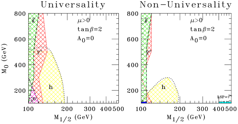
Figure 1: Excluded region in the $M_{0}$-$M_{1/2}$ plane from the experimental bounds of the SUSY particles. We have chosen the values displayed in the figure for the other input parameters. The excluded regions are denoted with the shaded ones and the particle which fails to pass the bound of Table I. Small shaded regions in the non-universality case indicate excluded regions from neutralinos and scalar $\tilde{\tau}$’s (left) and $\tilde{\tau}$ as an LSP (right).

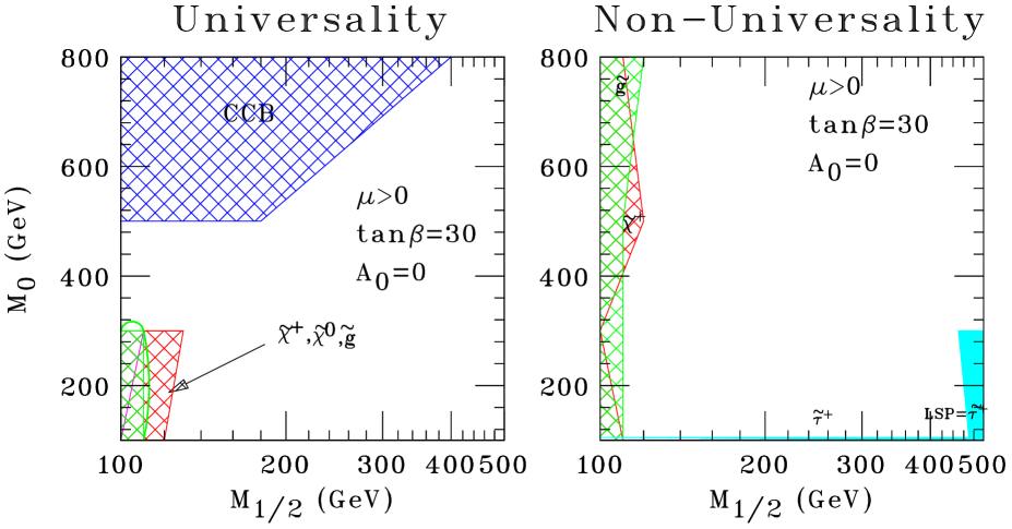
Figure 2: The same as Fig.1 with $\tan\beta=30$.

Figure 3: Predictions for the light top and bottom scalar quark masses as a function of $M_{1/2}$ for different values of $M_{0}$ (displayed) and $\tan\beta$=2(solid) 30(dot-dashed) values.

Figure 4: Predictions for the light tau scalar lepton and for the light Higgs boson masses as a function of $M_{1/2}$ for different values of $M_{0}$ (displayed) and $\tan\beta$=2(solid) 30(dot-dashed) values.

Figure 5: Predictions for the lightest neutralino (LSP) and chargino masses as a function of $M_{1/2}$ for different values of $M_{0}$ (displayed) and $\tan\beta$=2(solid) 30(dot-dashed) values.

Figure 6: Resulting values of the strong coupling $\alpha_{s}(M_{Z})$ as a function of $M_{0}$ for different values of the $M_{0}$. The top quark mass 175 GeV is assumed. We display results for both regions of small $\tan\beta=2$ (solid lines) and large $\tan\beta=30$ (dot-dashed) lines).

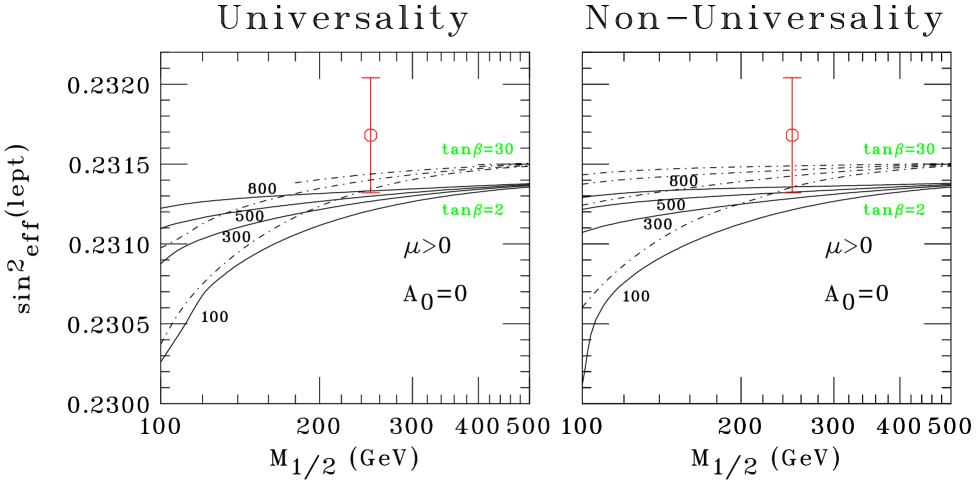
Figure 7: Resulting values of the effective (leptonic) weak mixing angle, $\sin^{2}_{eff}$(lept) as a function of $M_{1/2}$ for different values of the $M_{0}=$100,300,500,800 GeV and two different values of $\tan\beta=$2,30 (dot-dashed lines). The LEP experimental value is also shown.

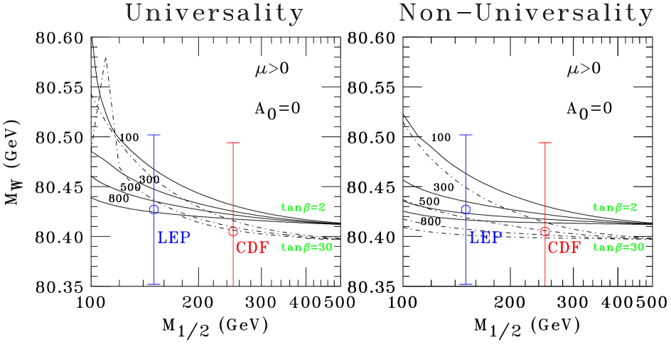
Figure 8: Resulting values of the physical W-pole mass, $M_{W}$ as a function of $M_{1/2}$ for different values of the $M_{0}=$100,300,500,800 GeV and two different values of $\tan\beta=$2,30 (dashed lines). The experimental CDF and DØ values are also displayed.

References

- [1] I. Antoniadis, J. Ellis, J. Hagelin and D.V. Nanopoulos, Phys. Lett. B231 (1989) 65; J.L. Lopez, D.V. Nanopoulos and K. Yuan, Nucl. Phys. B399 (1993) 654.
- [2] A.E. Faraggi, D.V. Nanopoulos, and K. Yuan, Nucl. Phys. B335 (1990) 347.
-
[3]
I. Antoniadis, G.K. Leontaris and J. Rizos, Phys. Lett. B245 (1990) 161;
G.K. Leontaris, Phys. Lett. B372 (1996) 212;
G.K. Leontaris and J. Rizos, hep-th/9901098. - [4] A.E. Faraggi, Phys. Lett. B278 (1992) 131; Nucl. Phys. B387 (1992) 239.
- [5] A.E. Faraggi, Phys. Lett. B274 (1992) 47; Phys. Lett. B339 (1994) 223.
- [6] G.B. Cleaver, A.E. Faraggi and D.V. Nanopoulos, Phys. Lett. B455 (1999) 135; hep-ph/9904301.
-
[7]
X.G. Wen and E. Witten, Nucl. Phys. B265 (1985) 651;
G.G. Athanasiu, J.J. Atick, M. Dine, and W. Fischler, Phys. Lett. B214 (1988) 55;
A.N. Schellekens, Phys. Lett. B237 (1990) 363;
J. Ellis, J.L. Lopez and D.V. Nanopoulos, Phys. Lett. B247 (1990) 257;
S. Chang, C. Coriano and A.E. Faraggi, Phys. Lett. B397 (1997) 76; Nucl. Phys. B477 (1996) 65. -
[8]
S. Chaudhoury, G. Hockney and J. Lykken,
Nucl. Phys. B469 (1996) 357;
G.B. Cleaver et. al. , Nucl. Phys. B525 (1998) 3; Nucl. Phys. B545 (1998) 47; Phys. Rev. D59 (1999) 055005; Phys. Rev. D59 (1999) 115003. -
[9]
K. Benakli, J. Ellis and D.V. Nanopoulos, Phys. Rev. D59 (1999) 047301;
A.E. Faraggi, K.A. Olive and M. Pospelov, hep-ph/9906345. -
[10]
M. Dine, R. Rohm, N. Seiberg and E. Witten,
Phys. Lett. B156 (1985) 55;
J.P. Derendinger, L.E. Ibanez and H.P. Nilles, Phys. Lett. B155 (1985) 65;
H.P. Nilles, Phys. Lett. B115 (1982) 193. - [11] V. Kaplunovsky and J. Louis, Phys. Lett. B306 (1993) 269.
- [12] M. Dine, A.E. Nelson, Y. Nir and Y. Shirman, Phys. Rev. D53 (1996) 2658.
-
[13]
P. Fayet, Nucl. Phys. B90 (1975) 104;
I. Antoniadis, John Ellis, A.B. Lahanas and D.V. Nanopoulos, Phys. Lett. B241 (1990) 24;
A.E. Faraggi, E. Halyo, Int. J. Mod. Phys. A11 (1996) 2357;
G. Dvali and A. Pomarol, Phys. Rev. Lett. 77 (1996) 3728;
P. Binetruy and E. Dudas, Phys. Lett. B389 (1996) 503. R. Mohapatra and A. Riotto, Phys. Rev. D55 (1997) 1138; N. Arkani–Hamed, M. Dine and S.P. Martin, Phys. Lett. B431 (1998) 239;
T. Barreiro, B. de Carlos, J.A. Casas and J.M. Moreno, Phys. Lett. B445 (1998) 82;
N. Irges, Phys. Rev. D59 (1999) 115008. - [14] A.E. Faraggi and J.C. Pati, Nucl. Phys. B526 (1998) 21.
- [15] L. Ibanez and D. Lust, Nucl. Phys. B382 (1992) 305.
-
[16]
G.B. Cleaver and A.E. Faraggi, Int. J. Mod. Phys. A14 (1999) 2335;
A.E. Faraggi, Phys. Lett. B426 (1998) 315; hep-ph/9807341. -
[17]
H. Kawai, D.C. Lewellen, and S.-H.H. Tye, Nucl. Phys. B288 (1987) 1;
I. Antoniadis, C. Bachas, and C. Kounnas, Nucl. Phys. B289 (1987) 87;
I. Antoniadis and C. Bachas, Nucl. Phys. B298 (1988) 586. -
[18]
L. Dixon, E. Martinec, D. Friedan and S. Shenker,
Nucl. Phys. B282 (1987) 13;
M. Cvetic, Phys. Rev. Lett. 59 (1987) 2829. - [19] S. Kalara, J.L. Lopez and D.V. Nanopoulos, Nucl. Phys. B353 (1991) 650.
-
[20]
A.E. Faraggi and D.V. Nanopoulos, Phys. Rev. D48 (1993) 3288;
A.E. Faraggi, Nucl. Phys. B407 (1993) 57; hep-th/9511093; hep-th/9708112. - [21] A.E. Faraggi, Phys. Lett. B326 (1994) 62.
- [22] I. Antoniadis, J. Ellis, S. Kelley and D.V. Nanopoulos, Phys. Lett. B272 (1991) 31.
-
[23]
M.K. Gaillard and R. Xiu, Phys. Lett. B296 (1992) 71;
A.E. Faraggi, Phys. Lett. B302 (1993) 302;
S.P. Martin and P. Ramond, Phys. Rev. D51 (1995) 6515. - [24] E. Witten, Nucl. Phys. B471 (1996) 135.
-
[25]
A.E. Faraggi, S. Kelley, J. Hagelin and D.V. Nanopoulos,
Phys. Rev. D45 (1992) 3272;
S.P. Martin and P. Ramond, Phys. Rev. D48 (1993) 5365;
Y. Kawamura, H. Murayama and M. Yamaguchi, Phys. Lett. B324 (1994) 52;
J.L. Feng, M.E. Peskin, H. Murayama and X. Tata, Phys. Rev. D52 (1995) 1418;
Y. Kawamura, T. Kobayashi and T. Komatsu, Phys. Lett. B400 (1997) 284. - [26] A. Dedes, A.B. Lahanas and K. Tamvakis, Phys. Rev. D59 (1999) 015019.
- [27] A. Dedes, A.B. Lahanas, J. Rizos and K. Tamvakis, Phys. Rev. D55 (1997) 2955.
- [28] A.E. Faraggi and B. Grinstein, Nucl. Phys. B422 (1994) 3.
- [29] J. Bagger, K. Matchev and D. Pierce, Phys. Lett. B348 (1995) 443.
- [30] A.B. Lahanas and K. Tamvakis, Phys. Lett. B348 (1995) 451.
- [31] A. Dedes, A.B. Lahanas and K. Tamvakis, Phys. Rev. D53 (1996) 3793.
- [32] G. Abbiendi et al. [OPAL Collaboration], Eur. Phys. J. C8 (1999) 255.
- [33] C. Caso et al., The European Physical Journal C3 (1998) 1.
- [34] G. Abbiendi et al. [OPAL Collaboration], hep-ex/9808036.
- [35] P. Abreu et al. [DELPHI Collaboration], Phys. Lett. B444 (1998) 491.
- [36] B. Abbott et al. [D0 Collaboration], hep-ex/9902013.
- [37] S. Navas-Concha, ’MSSM searches at LEP’, talk given at ‘SUSY 98’, Keble College, Oxford, UK, July 11-17 1998.
-
[38]
J. Valls, ‘MSSM and Higgs Search at the Tevatron’, XXIX ICHEP’98,
Vancouver Conference, July 1998;
K. De, ’MSSM searches at the Tevatron’, talk given at ‘SUSY 98’, Keble College, Oxford, UK, July 11-17 1998. - [39] B. Abbott et al. [D0 Collaboration], hep-ex/9903041.
- [40] A. Hocker, hep-ex/9903024.
- [41] B. Abbott et al. [D0 Collaboration], hep-ex/9902028.
- [42] T. Falk, K.A. Olive, L. Roszkowski and M. Srednicki, Phys. Lett. B367 (1996) 183.
- [43] S.P. Martin and M.T. Vaughn, Phys. Rev. D50 (1994) 2282.
- [44] Y. Yamada, Phys. Rev. D50 (1994) 3537.
- [45] I. Jack and D.R. Jones, Phys. Lett. B349 (1995) 294.
- [46] I. Jack, D.R. Jones and K.L. Roberts, Nucl. Phys. B455 (1995) 83.
- [47] K.R. Dienes and A.E. Faraggi, Nucl. Phys. B457 (1995) 409.
- [48] G. Altarelli, hep-ph/9811456.