Coherent States in High-Energy Physics

Abstract

The amplitude for emitting $n$ bosons factorizes into the product of $n$ single-boson emission amplitudes, if the source is energetic and abelian. If it is energetic but non-abelian, the amplitude is given by a sum of factorized quasi-particle amplitudes. A quasi-particle is made up of an arbitrary number of bosons, but couples to the source like a single one. Factorization is related to coherence, and it allows computation of subleading contributions not obtainable by usual means. Its importance is illustrated in two applications: to solve the baryon problem in large-$N_{c}$ QCD, and to obtain a total cross section satisfying the Froissart bound.

I Introduction

We found a quasi-particle state of gluons whose existence has eluded detection all these years. In this talk I will discuss how that comes about, and what use we can make of it. A quasi-particle is made up of an arbitrary number of gluons, but it couples to their high-energy source like a single one: as a colour-octet object whose emission preserves helicity of the source. Quasi-particles emerge naturally as a result of factorization and coherence. They are present in all non-abelian theories, including the Yukawa theory of nucelons and pions, and not just QCD.

By a high-energy source, I mean a source with large total energy. The source may be a highly relativistic particle with a small mass, or a non-relativistic particle with a very large mass. For simplicity, I shall refer to these two cases respectively as a relativistic source and a non-relativistic source.

By a non-abelian theory, I mean one in which the spin and/or the internal quantum numbers of the high-energy source can be altered by the emission of bosons. In the case of pions emitted from a massive non-relativistic nucleon, it is the spin and the isospin of the nucleon that are affected by the emission. In the case of QCD it is the colour of the source. But in the case of photons emitted from a relativistic electron, neither the charge nor the helicity of the electron is changed, so in this case the source is abelian.

After sketching the origin of the quasi-particle, and its connection with factorization and cohernece, I will discuss two cases in which it makes its presence felt. I believe these applications barely scratch the surface, and the importance of these quasi-particles goes far beyond these two examples, but exactly in what way remains to be seen.

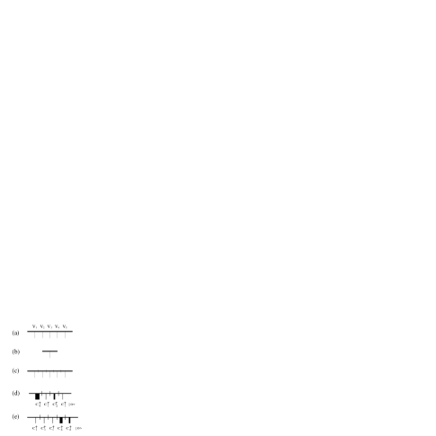
FIGURE 1.: (a). A Feynman tree amplitude with vertex factors $V_{i}$; (b). A one-boson amplitudes with on-shell sources; (c). The factorization of a Bose-Einstein symmetrized amplitude into the product of one-boson amplitudes; (d) and (e). Two separate factorization into quasi-particle amplitudes.

II The Emergence of Quasi-Particles

Consider the tree diagram Fig. 1(a), in which $n$ bosons are emitted from an energetic source via vertex factors $V_{i}$. The source is assumed to be energetic so that recoils suffered from the emissions can be ignored. As a result, its transverse position $x_{\perp}$ is fixed, and so is the $x_{\perp}$ of every boson emerging from it. In the case of a relativistic source, we may assume it to move parallel to the $z$-axis near the speed of light, hence its $x^{-}\equiv x^{0}-x^{3}$ coordinate is fixed, thereby determining also the $x^{-}$ coordinate of all the emerging bosons. For a non-relativistic source, its $x^{3}$ coordinate and that of the bosons are fixed. All in all, three out of four coordinates of all the off-shell bosons are identical. If the fourth one is also the same for all the bosons, a coherent state will emerge. It turns out that non-trivial inputs are required to determine this fourth coordinate to achieve coherence.

It is necessary to invoke Bose-Einstein symmetry, which in this case simply means summing up the $n!$ permuted tree amplitudes. For abelian sources, the vertices $V_{i}$’s can be regarded simply as numbers. In that case we will show that every boson of the BE-symmetrized amplitude has its momentum component $k^{-}=k^{0}-k^{3}=0$ if the source is relativistic, and $k^{0}=0$ if the source is non-relativistic. This is the fourth coordinate we are after for a coherent state.

The conclusion follows as a result of factorization. After the summation, each boson is allowed to be emitted anywhere along the tree, irrespective of the location of the others. Hence the $n$-boson amplitude is factorized into a product of $n$ single-boson emission amplitudes. This is depicted in Fig. 1(c), where a vertical cut on the tree indicates factorization. For a relativistic source that is on-shell, its momentum component $p^{-}=p^{0}-p^{3}=0$, so by momentum conservation (see Fig. 1(b)) $k^{-}=0$ for every boson as claimed. For a non-relativistic source that is on-shell, $p^{0}$ is fixed at its on-shell mass $M$, so by momentum conservation $k^{0}=0$. Note that neither conclusion is valid for the boson momenta in a Feynman diagram like Fig. 1(a), where off-shell sources are involved. In that case, uncertainty in energy prevents $p^{-}$ or $p^{0}$ to be fixed, so it is not true that $k^{-}$ or $k^{0}$ is zero. Bose-Einstein symmetrization and the resulting factorization are crucial to reach these conclusions.

Note also that this kind of coherent state is very different from those encountered at low temperatures, where Bose-Einstein condensation may occur. The coherent state we have is described by a mixture of spatial and momentum coordinates, and it is not an energy eigenstate. What is ‘cold’ in the present context is the lack of recoil, instead of the lack of thermal fluctuation. Hence the physics outcome between the two are completely different as well.

For non-abelian sources this simple factorization is no longer valid. The vertex factors $V_{i}$ fail to commute with one another, so correction terms involving their commutators must be added  [?]. It turns out that each of these correction terms is still factorizable, but generally into products of quasi-particle amplitudes instead of single-boson amplitudes. In other words, it is the $k^{-}$ or the $k^{0}$ coordinates of the quasi-particles as a whole that are zero, but not the individual bosons within each quasi-particle. As remarked before, a quasi-particle may consist of any number $k$ of bosons, but instead of coupling to the source via the product of vertex factors $V_{1}V_{2}\cdots V_{k}$, it does so via the nested commutator $[V_{1},[V_{2},[\cdots,[V_{k-1},V_{k}]\cdots]]]$. In the case of QCD when $V_{i}$ are colour matrices, the nested commutator is given by a linear sum of colour matrices, so the quasi-particle couples just like a colour-octet object. Moreover, since each gluon making up the quasi-particle does not flip the helicity of the source, neither will the quasi-particle.

Exactly how each correction term factorizes depends on the permutation. I list here three examples for $n=8$: $[1|2|3|4|5|6|7|8],\ [8521|3|74|6],\ [1|2|3|864|75]$, in which a vertical bar indicates the position where factorization takes place. The general rule is simply that a bar should be put behind a number iff no number to its right is smaller than it. The first example is identical to abelian factorization. In the second example, the source emits a quasi-particle of four gluons, one of two gluons, and two with one gluon each (a quasi-particle with one gluon is just a gluon). In the third example, there are three quasi-particles with one gluon each, one with three gluons, and one with two gluons. The last two examples involve nested commutators so they will not be present for abelian sources. In fact, other than the first example, no other permutation can contribute in the case of an abelian source for exactly the same reason.

Letting $Q$ denote a quasi-particle, the general structure of each factorized amplitudes is therefore of the form

$$[Q|Q|\cdots|Q],$$ (1)

where the different quasi-particles $Q$ appearing in this equation may consist of different number of gluons.

III Composite Source

Suppose the source is made up of $N$ constituents, each capable of emitting a boson via the vertex $V_{i}=\psi^{\dagger}t_{i}\psi$, where $\psi$ and $\psi^{\dagger}$ are the annihilation and creation operators for the constituents. For example, the source may be a nucleus with $N$ nucleons, or a nucleon with $N$ quarks. Being a one-body operator, the matrix elements of $V_{i}$ is expected to be of order $N$. Being a $k$-body operator, the matrix element of a product of $k$ $V_{i}$’s is expected to be of order $N^{k}$. In contrast, the nested commutator of $k$ $V_{i}$’s is of the form $\psi^{\dagger}T\psi$, with $T$ given by the nested commutator of the $t_{i}$’s, so it is still a one-body operator and its matrix element is proportional to $N$. If the an $n$-boson amplitude in (1) contains $p$ quasi-particles, then that term is of order $N^{p}$, with $p\leq N$, and not $N^{n}$ that each Feynman tree diagram is expected to have. Except for the identical permutation whose amplitude factorizes completely as in $[1|2|3|\cdots|n]$, so that $p=n$, all the others have $p<n$ and hence contribute subdominantly when $N\gg 1$. The smaller $p$ is the less it contributes. If for some reason all the terms with $n\geq p\geq p_{0}+1$ vanish, then the amplitude is of order $N^{p_{0}}$. It can still be computed easity from the quasi-particle amplitudes with $p\leq p_{0}$, but it is extremely difficult to calculate it directly from Feynman tree diagrams, especially when $p^{0}\ll n$. To do so we must compute each Feynman diagram to the subleading order $N^{p_{0}}$ before a finite sum can be obtained upon summation, a highly non-trivial task.

Such a behaviour indeed happens in the process $\pi+{\cal N}\to(n-1)\pi+{\cal N}$, calculated in large-$N$ QCD  [?]. In that case, the nucleon ${\cal N}$ consists of $N$ quarks. Its mass is of order $N$ so it is a non-relativistic energetic source. The effective Yukawa interaction $t=g(\vec{\sigma}\cdot\vec{k})(\vec{\tau}\cdot\vec{\pi}(\vec{k}))$ is non-abelian because it flips the spin and the isospin of the nucleon. Each Feynman tree amplitude is of order $N^{n}/\sqrt{N}^{n}$ because it consists of $n$ vertices and the propagators are of order 1. A normalization factor $1/\sqrt{N}$ per pion is put in as usual  [?]. The amplitude is huge for every $n>0$ in the limit $N\gg 1$. In this strong-coupling limit one might think that very little could be said about the reaction, and certainly the Feynman-diagram description is useless even when loops are included. Yet the phenomenology of baryons in large-$N$ QCD is very successful in describing nature  [?]. What happens is that when the $n!$ permuted diagrams are summed up, a tremendous amount of cancellation takes place, so that the final $n$-pion amplitude is of order $N^{1-n/2}$ rather than $N^{n/2}$ of the individual diagrams. The total pion-nucleon amplitudes now become weak for $n>2$, so we can understand why loops are not needed and why phenomenology can be successful. In order to prove this cancellation in a brute-force way, each diagram must be calculated down to $(n-1)$ subleading orders, for at the end everything else above it will be cancelled in the sum. This is quite an impossible task for large $n$, and this is where the advantage of the factorized formula (1) shows up  [?]. If the number $p$ of quasi-particle amplitudes in (1) is larger than 1, then it vanishes because of energy conservation. In that case one of these $p$ factorized components must consist of only outgoing pions, which violates energy conservation since the nucleons are on-shell. As a result we are left with only terms with $p=1$, whose matrix element is $N/\sqrt{N}^{n}=N^{1-n/2}$, as claimed.

IV Damping Explosive Total Cross Sections

Total cross section can be obtained from the forward elastic amplitude via the optical theorem. This amplitude is difficult to compute even assuming the coupling constant $\alpha_{s}$ to be small, for at high cm energy complicated loop diagrams must be included. This is so because each time we add a loop to the diagram, we add an extra factor of $\alpha_{s}$ but the loop integration may also produce an extra $\ln s$. Thus a diagram of order $2n+2$ may give a contribution proportional to $\alpha_{s}(\alpha_{s}\ln s)^{n}$, which is of order $\alpha_{s}$ if $\xi\equiv\alpha_{s}\ln s=O(1)$. This is why diagrams of all orders must be included.

Computing multi-loop diagram is a difficult task which can be accomplished only with suitable approximations. In the leading-log approximation, which keeps only the lowest power of $\alpha_{s}$ while keeping the variable $\xi$ fixed, the total cross section so computed is proportional to $\alpha_{s}^{2}\exp(4\alpha_{s}\ln s\ln 2N_{c}/\pi)$. This is the famous BFKL formula  [?]. With $\alpha_{s}\simeq 0.19$, for example, the cross section according to this formula grows with energy like $s^{0.5}$. At this rate the size of a proton becomes ten times the size of the Uranium nucleus at LHC energy, and one hundred times its size at $10^{20}$ eV, the highest energy cosmic-ray reaching earth. For better or for worse, this alarming growth is not realized. In fact, Froissart bound forbids the total cross section to grow faster than $\ln^{2}s$ at asymptotic energies. The theoretical challenge then is how to produce sufficient amount of corrections in QCD to satisfy the Froissart bound. Since the BFKL computation already includes all the important contributions in the leading-log approximations, viz., all terms of order $\alpha_{s}^{2}$ when $\xi$ is kept fixed, clearly subleading terms of order $\alpha^{m}$ with $m\geq 3$ are needed for the Froissart bound. As explained in the last section, the factorization formula (1) is capable of extracting subleading terms $N^{p}$ for $p<n$ in that case. Similarly, (1) can be used to extract subleading terms $\alpha_{s}^{m}$ with $m\geq 3$  [?]. The result is shown in Fig. 1(b), where the thick vertical lines represent quasi-particles, and the thin vertical cuts on the two horizontal lines represent factorization. It can be shown that an amplitude with $p$ vertical quasi-particle lines is of order $\alpha_{s}^{p}$; this is analogous to the situation of the last section in which an amplitude with $p$ quasi-partilces is proportional to $N^{p}$.

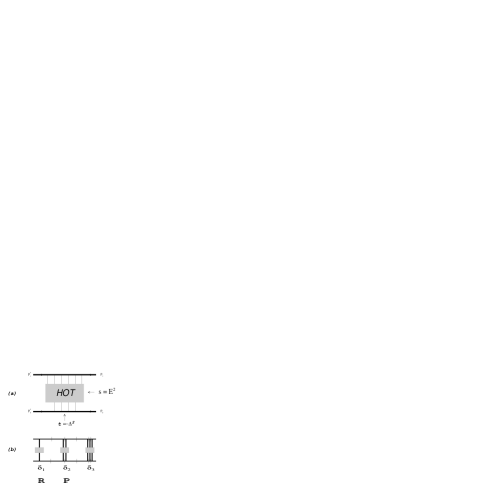
FIGURE 2.: (a). A two-particle collision diagram showing a hot central region and a ‘cold’ peripheral region; (b). Factorization of the scattering amplitude into quasi-particle amplitudes. An amplitude with $p$ quasi-particle exchanges can be shown to be of order $\alpha_{s}^{p}$ if $\alpha)s\ln s$ is of order 1.

For $\alpha_{s}\ll 1$ and $\xi=O(1)$, the dominant scattering amplitude comes from diagrams with $p=1$ (alone), indicated in Fig. 2(b) by $\delta_{1}$. Remebering that each quasi-particle carries an octet colour, we conclude that the dominant amplitude is a colour-octet amplitude (in the $t$-channel), whose magnitide is $O(\alpha_{s})$. It has been known long ago  [?] that the dominant amplitude is obtained by the exchange of a colour-octet Reggeon, so from these two equivalent descriptions we can identify the quasi-particle with the Reggeon. What has thus been achieved here is an algebraic characterization of the Reggeon, as the colour-octet object obtained through factorization and coherence, rather than a pole in the angular momentum plane as is usually defined.

A quasi-particle in QCD is not the same as a gluon, but a quasi-particle in QED is identical to a photon because all the nested commutators vanish. This distinction is ultimately the reason why gluons reggeize but photons do not.

Total cross section is related to the forward part of the elastic scattering amplitude, so only the exchange of colour-singlet object contributes to it. The dominant amplitude then comes from the exchange of two interacting Reggeons, indicated by $\delta_{2}$ in Fig. 2(b), or two non-interacting Reggeons $\delta_{1}^{2}$. The result is of order $\alpha_{s}^{2}$, and it is the BFKL Pomeron  [?], which as mentioned before violates unitarity. $s$-channel unitarity and the Froissart bound are restored when we incorporate the singlet part of $p$-Reggeon exchanges, with all $p\geq 3$ included. For virtual-photon proton total cross section, as measured at HERA  [?], this results in a shallower growth of total cross section with energy for a smaller virtuality $Q^{2}$ of the virtual photon, as shown in Fig. 3.

For details see Ref.  [?].

Finally one might ask why coherence should have anything to do with high-energy collisions. After all, the centre of collision will be hotter than the centre of a star (Fig. 2(a)), whereas Bose-Einstein coherence usually happens at low temperature. The answer is that although the centre is hot, the peripheral regions are ‘cold’, and that is sufficient to produce factorization as indicated in Fig. 2(b).

FIGURE 3.: Energy dependence of $\gamma^{*}p$ total cross section as a function of photon virtuality $Q^{2}$. Data is from Ref. [8]. The dotted line represents a dependence of $s^{0.08}$ obeyed by all hadronic total cross sections. The dash line gives a $s^{0.5}$ variation predicted by the leading-log BFKL Pomeron, and the solid line is the prediction of the unitary theory in Ref. [6].

REFERENCES

REFERENCES

- 1. Lam C.S., and Liu K.F., Nucl. Phys. B483, 514 (1997); Feng Y.J., Hamidi-Ravari O., and Lam C.S., Phys. Rev. D 54, 3114 (1996); Lam C.S., J. Math. Phys. 39, 5543 (1998).
- 2. ’t Hooft G., Nucl. Phys. B72, 461 (1974); Coleman S., Erice Lectures (1979); Witten E., Nucl. Phys. B160, 57 (1979).
- 3. Dashen R.F., Jenkins E., and Manohar A.V., Phys. Rev. D 49, 4713; Phys. Rev. D 51, 3657 (1995); Dashen R., and Manohar A.V., Phys. Lett. B 315, 425, 438 (1993); Jenkins E., Phys. Lett. B 315, 431, 441, 447 (1993); Luty M.A., and March-Russell J., Nucl. Phys. B426, 71 (1994); Luty M.A., Phys. Rev. D 51, 2322 (1995).
- 4. Lam C.S., and Liu K.F., Phys. Rev. Lett. 79, 597 (1997).
- 5. Lipatov L.N., Sov. J. Nucl. Phys. 23, 338 (1976); Balitskii Ya., and Lipatov L.N., Sov. J. Nucl. Phys. 28, 822 (1978); Kuraev E.A,, Lipatov L.N., and Fadin V.S., ZSov. Phys. JETP 44, 443 (1976); ibid. 45, 199 (1977).
- 6. Dib R., Khoury J., and Lam C.S., hep-ph/9902429, to appear in Phys. Rev. D.
- 7. For a review, see Cheng H., and Wu T.T., ‘Expanding Protons: Scattering at High Energies’, (M.I.T. Press, 1987); Del Duca V., hep-ph/9503226.
- 8. ZEUS Collaboration, hep-ex/9707025.