SLAC–PUB–8188

ETH-TH/99-10

DTP/99/72

hep-ph/9907305

July 1999

Vector Boson Pair Production in Hadronic Collisions at ${\cal O}(\alpha_{s})$: Lepton Correlations and Anomalous Couplings

L. Dixon Stanford Linear Accelerator Center, Stanford University, Stanford, CA 94309, USA
Z. Kunszt Theoretical Physics, ETH Zürich, Switzerland
A. Signer Department of Physics, University of Durham, Durham DH1 3LE, England

We present cross sections for production of electroweak vector boson pairs, $WW$, $WZ$ and $ZZ$, in $p\bar{p}$ and $pp$ collisions, at next-to-leading order in $\alpha_{s}$. We treat the leptonic decays of the bosons in the narrow-width approximation, but retain all spin information via decay angle correlations. We also include the effects of $WWZ$ and $WW\gamma$ anomalous couplings.

Submitted to Physical Review D

1 Introduction

At the core of the electroweak Standard Model is its invariance under the nonabelian gauge group $SU(2)\times U(1)$. Many aspects of this gauge structure, such as vector boson masses and couplings to fermions, have already been tested with high precision in a variety of experiments. However, the nonabelian self-interactions of vector bosons — in particular, triple gauge-boson couplings — are just beginning to be studied directly, via vector-boson pair production in $e^{+}e^{-}$ annihilation at LEP2 at CERN, and in $p\bar{p}$ collisions at Run I of the Fermilab Tevatron. Although thousands of $W^{+}W^{-}$ pairs have been collected at LEP2, they have all been produced at relatively modest values of the pair invariant mass, $M_{WW}\raisebox{1.99997pt}{$\hbox to0.0pt{\raisebox{-5.0pt}{$\;\sim$}\hss}<\,$}200$ GeV. On the other hand, if there are anomalous (non-Standard Model) vector-boson self-couplings, their effects are expected to grow with invariant mass, so it is useful to study vector-boson pair production at the highest possible energies. Vector boson pairs also provide a background for other types of physics. If the Higgs boson is heavy enough it will decay primarily into $W^{+}W^{-}$ and $ZZ$ pairs [1]. Exotic Higgs sectors can have substantial branching ratios for charged Higgs bosons to decay to $WZ$ pairs [2]. Leptonically decaying $WZ$ pairs, $W^{+}Z\to\ell^{+}\nu\ell^{\prime+}\ell^{\prime-}$, in which the negatively-charged lepton is lost, form a background to a signal for strong $WW$ scattering associated with the mode $W^{+}W^{+}\to\ell^{+}\nu\ell^{\prime+}\nu^{\prime}$ [3]. Finally, a prime signal for supersymmetry at hadron colliders is the production of three charged leptons and missing transverse momentum [4]; a background for this process is the production of a $W$ plus a (virtual) $Z$ or $\gamma$.

In the near future, hadron colliders will be the primary source of vector boson pairs with large invariant mass. Run II of the upgraded Tevatron should yield a data set roughly 20 times larger than that from Run I, including 100–200 leptonically decaying $W^{+}W^{-}$ pairs. The Large Hadron Collider (LHC) at CERN promises to increase the sample by another factor of 50 beyond Run II. With this increase in statistics, refined Standard Model predictions are essential. The leading QCD corrections (${\cal O}(\alpha_{s})$) are significant (generally of order tens of percent), and hence are required to get a precise estimate of the overall production cross section. Also, experiments do not detect vector bosons, but only those leptonic decay products that fall within the experimental acceptance. Spin correlations between vector bosons are reflected in kinematic distributions of leptonic momenta, which in turn influence the number of events surviving experimental cuts. In order to properly take into account the effects of cuts on the cross section, as well as to study the more detailed (lepton) kinematic distributions permitted by higher statistics, it is important to treat the vector boson decays properly, including all spin correlations.

Hadronic production of vector boson pairs in the Standard Model has already been studied extensively. The Born-level, or leading-order (LO) cross sections for $W^{+}W^{-}$, $W^{\pm}Z$ and $ZZ$ pair production via quark annihilation were computed twenty years ago [6]. These cross sections were evaluated by treating the $W$ and $Z$ as stable particles and summing over their polarization states, using completeness relations to simplify the sum; thus spin and decay correlations were neglected. For the spin-summed production cross section, the next-to-leading order (NLO, or ${\cal O}(\alpha_{s})$) QCD corrections were obtained for $W^{+}W^{-}$ final states in refs. [7, 8], for $W^{\pm}Z$ in refs. [9, 10], and for $ZZ$ in refs. [11, 12].

The simplest way to include the effects of vector-boson spin and decay correlations is to compute directly the matrix elements for the production of the four final-state fermions. In the narrow-width approximation, only ‘doubly-resonant’ Feynman diagrams have to be considered — the same class of diagrams that gives rise to the on-shell spin-summed cross section. Because both the outgoing fermions and the initial-state partons are essentially massless, and because their couplings to vector bosons are chiral, it is very convenient to use a helicity basis for the fermions. The tree-level helicity amplitudes for massive vector-boson pair production and decay into leptons were first computed in ref. [13], which also demonstrated the significance of decay-angle correlations. This same approach was carried out at order $\alpha_{s}$ in ref. [14]. At ${\cal O}(\alpha_{s})$, there are real corrections, consisting of tree graphs with an additional gluon in either the initial or final state, and virtual corrections, consisting of one-loop amplitudes that interfere with the Born amplitude. However, the full one-loop amplitudes including leptonic decays were unavailable until recently, so ref. [14] included decay correlations everywhere except for the finite part of the virtual contribution, for which spin-summed formulae were used.

In this paper, we present ${\cal O}(\alpha_{s})$ results for the hadronic production of $W^{+}W^{-}$, $WZ$ and $ZZ$ pairs, including the full lepton decay correlations in the narrow-width approximation. We rely on ref. [15] for all the required matrix elements, in particular the virtual one-loop amplitudes for $q\bar{q}^{\prime}\to V_{1}V_{2}\to 4$ leptons. In order to cancel the infrared divergences in the phase-space integrations for the real corrections, we implement the general subtraction method discussed in ref. [16]. This method allows the computation of distributions of arbitrary (infrared-safe) observables.

Recently, an update to vector boson pair production has been presented in ref. [17]. The corresponding Monte Carlo program, MCFM, relies on the same amplitudes [15] and, therefore, also includes all spin correlations exactly to next-to-leading order in $\alpha_{s}$. MCFM is more complete than the program described here, in the sense that the narrow-width approximation is not assumed, and singly-resonant diagrams are also included. These additions are expected to shift the resonance-dominated di-vector boson cross sections by the order of several percent. Their effects are obviously much bigger in the off-resonant regions important for studies of Standard Model backgrounds to new physics.

In the present paper, we first compute the di-vector boson cross sections in the Standard Model, both without and with a realistic set of experimental cuts. For $W^{+}W^{-}$ production, a jet veto is used by experimentalists to suppress backgrounds; we study the effect of this veto on the size of the cross section and its renormalization/factorization scale dependence.

Di-boson amplitudes in the Standard Model have interesting angular dependences. For example, at Born level, there is an exact radiation zero in the partonic process $q_{1}\bar{q}_{2}\to W^{\pm}\gamma$ at $\cos\theta=(Q_{1}+Q_{2})/(Q_{1}-Q_{2})$, where $\theta$ is the scattering angle of the $W$ with respect to the direction of the quark $q_{1}$, and $Q_{1,2}$ are the quark electric charges [6]. Similarly, it has been shown that there is a an approximate zero for $q_{1}\bar{q}_{2}\to W^{\pm}Z$ at $\cos\theta=(g^{-}_{1}+g^{-}_{2})/(g^{-}_{1}-g^{-}_{2})$, where $g^{-}_{1,2}$ are the left-handed couplings of the $Z$ boson to the quarks [18]. The exact tree-level zero for $W\gamma$ is filled in somewhat by QCD radiative corrections, and also by the kinematic ambiguity associated with the undetected neutrino in $W^{+}\gamma\to\ell^{+}\nu\gamma$. Still it produces a dip in the distribution of a related variable, the rapidity difference $y_{\gamma}-y_{\ell^{+}}$, which should be visible at Run II [19].

Here we study the QCD corrections to the approximate $WZ$ radiation zero. Using on-shell, spin-summed cross sections, ref. [10] computed the distribution in the rapidity difference between the $W$ and $Z$ bosons, $\Delta y_{WZ}=|y_{W}-y_{Z}|$, which is a boost-invariant surrogate for the center-of-mass scattering angle $\theta$. It was found that a dip in the $\Delta y_{WZ}$ distribution persists at ${\cal O}(\alpha_{s})$, although the dip is less pronounced than at Born level. Since the rapidity of the $W$ cannot be determined on an event-by-event basis, we study a quantity related to $\Delta y_{WZ}$, but constructed purely out of charged lepton variables, and find that a dip (or at least a shoulder) is still present. However, because of the much lower $WZ$ cross section, this measurement is considerably more challenging than the $W\gamma$ case, and will probably have to wait for the LHC.

Various types of TeV-scale physics may modify vector-boson self-interactions. Without a precise knowledge of the new physics, one often parameterizes the modifications using anomalous coupling coefficients. We shall consider anomalous contributions to the $W^{+}W^{-}Z$ and $W^{+}W^{-}\gamma$ triple gauge vertices, and their effect on various distributions in $WW$ and $WZ$ production. Similar studies have already been carried out at order $\alpha_{s}$ and including spin correlations everywhere except in the finite virtual contributions, for both $WW$ production [20] and $WZ$ production [21]. Here we include as well the spin correlation effects from the finite virtual contributions. This requires matrix elements beyond those in ref. [15]; however, the new matrix elements are trivial by comparison.

The remainder of the paper is organized as follows. After outlining the computational techniques in section 2, we present results for the Standard Model production of $WW$, $WZ$ and $ZZ$ pairs in section 3. We first present total cross sections for all three channels, without and then with a set of realistic kinematic cuts on the leptons. We consider both $p\bar{p}$ collisions at $\sqrt{s}=2$ TeV (corresponding to Run II of the Tevatron), and $pp$ collisions at $\sqrt{s}=14$ TeV (the LHC). We discuss the dependence of the $WW$ cross section on a common renormalization and factorization scale, with and without a jet veto. For the $WZ$ channel, we study the approximate radiation zero before and after QCD corrections.

In section 4 we introduce anomalous $W^{+}W^{-}Z$ and $W^{+}W^{-}\gamma$ couplings, and compute their effect on the matrix elements in the narrow-width approximation through ${\cal O}(\alpha_{s})$. We then study the effects of these couplings on a double-binned transverse energy distribution for the pair of charged leptons in $W^{+}W^{-}$ production followed by leptonic decays. Finally, in section 5 we present our conclusions.

2 Computation

It is straightforward to implement the helicity amplitudes presented in ref. [15], and those including anomalous couplings (see section 4), in a Monte Carlo program. The tree-level and one-loop amplitudes are computed as complex numbers and the squaring, as well as the sum over helicity configurations, is done numerically. In order to cancel singularities between the real and virtual parts analytically, we use the general version of the subtraction method [22] as presented in ref. [16]. Our code is flexible enough to compute arbitrary infrared-safe quantities, apply arbitrary cuts, and add any parton distribution easily.

In this paper we will present results for the Tevatron Run II and the LHC. The former term refers to $p\bar{p}$ scattering at $\sqrt{s}=2$ TeV, whereas the latter stands for $pp$ scattering at $\sqrt{s}=14$ TeV. Most of our results will be presented with some ‘standard cuts’ which are defined as follows: We make a transverse momentum cut of $p_{T}>20$ GeV for all charged leptons. The event is required to have a minimum missing transverse momentum $p_{T}^{\rm miss}$, which is carried off by the neutrino(s). We require $p_{T}^{\rm miss}>25$ GeV in the case of $W$-pair production and $p_{T}^{\rm miss}>20$ GeV in the case of $W^{\pm}Z$ production. No $p_{T}^{\rm miss}$ cut is applied for $Z$-pair production. Finally, we apply some collider-dependent rapidity cuts for the charged leptons. For the Tevatron we require $|\eta|<1.5$, whereas for the LHC $|\eta|<2.5$.

In all results presented in this paper, we assume that the vector bosons always decay leptonically, i.e. the proper branching ratios of the vector boson decays into leptons ${\rm Br}(V\to f\bar{f}^{\prime})$ are not included. Obviously, these branching ratios depend on which final-state charged leptons are included in the analysis (electrons, muons, or both). They can easily be added at any stage, using

$${\rm Br}(Z\to e^{+}e^{-})={\rm Br}(Z\to\mu^{+}\mu^{-}) = 3.37\%,$$

$$\sum_{i=e,\mu,\tau}{\rm Br}(Z\to\nu_{i}\bar{\nu_{i}}) = 20.1\%,$$ (1)

$${\rm Br}(W^{+}\to e^{+}\nu_{e})=\ {\rm Br}(W^{+}\to\mu^{+}\nu_{\mu}) = 10.8\%.$$

These ratios implicitly incorporate QCD corrections to the hadronic decay widths of the $W$ and $Z$.

We use two different parton distributions, MRST(ft08a) [23] and CTEQ(4M) [24], which we refer to simply as MRST and CTEQ. For both the leading and next-to-leading order results we shall use the same parton distributions (which have been obtained by a fit at next-to-leading order in $\alpha_{s}$). The strong coupling constant is evaluated using

$$\alpha_{s}(\mu) = {\alpha_{s}(M_{Z})\over w}\left(1-\frac{\alpha_{s}(M_{Z})}{\pi}{\beta_{1}\over\beta_{0}}{\ln(w)\over w}\right)\,,$$

$$w = 1-\beta_{0}\frac{\alpha_{s}(M_{Z})}{\pi}\ln\biggl{(}{M_{Z}\over\mu}\biggr{)}\,,$$ (2)

with $\beta_{0}=\frac{1}{2}(\frac{11}{3}C_{A}-\frac{2}{3}N_{f})$, $\beta_{1}=\frac{1}{4}(\frac{17}{3}C_{A}^{2}-(\frac{5}{3}C_{A}+C_{F})N_{f})$, $C_{A}=N_{c}$, $C_{F}=(N_{c}^{2}-1)/(2N_{c})$. The value of $\alpha_{s}(M_{Z})$ is set equal to the value given in the respective parton distribution fit. Thus, we take $\alpha_{s}(M_{Z})=0.1175$ for MRST and $\alpha_{s}(M_{Z})=0.116$ for CTEQ. In all computations we have set the renormalization and factorization scales equal: $\mu_{R}=\mu_{F}\equiv\mu$.

The masses of the vector bosons have been set to $M_{Z}=91.187$ GeV and $M_{W}=80.33$ GeV. As for the coupling constants $\alpha$ and $\sin^{2}\theta_{W}$, we choose them in the spirit of the “improved Born approximation” [25, 26] for $W$ pair production at LEP2. We do not explicitly include any QED or electroweak radiative corrections. However, we take into account the top-quark-enhanced corrections to the relation between $M_{Z}$, $M_{W}$ and $\sin^{2}\theta_{W}$, where the latter is defined as an effective coupling in a high-energy process, by using the definition [26]

$$\sin^{2}\theta_{W}\equiv{\pi\alpha(M_{Z})\over\sqrt{2}G_{F}M_{W}^{2}}\,,$$ (3)

where $G_{F}=1.16639\times 10^{-5}$ GeV^-2 is the Fermi constant and $\alpha(\mu)$ the running QED coupling. For our numerical results we use $\alpha=\alpha(M_{Z})=1/128$ and $\sin^{2}\theta_{W}=0.230$.

The programs have been set up to allow for arbitrary values in the entries of the Cabibbo-Kobayashi-Maskawa (CKM) mixing matrix that do not depend on the top quark. For the numerical results we take $|V_{ud}|=|V_{cs}|=0.975$ and $|V_{us}|=|V_{cd}|=0.222$.

Finally we mention that we do not properly include processes where top quarks are involved. The amplitudes presented in ref. [15] assume massless quarks, an approximation that is certainly not justified in the case of the top quark. The fact that we nevertheless include the $t$-channel exchange of the top quark (with $|V_{td}|=|V_{ts}|=0$ and $|V_{tb}|=1$) for $W$-pair production, therefore, results in an error. Fortunately, these processes are suppressed for energy scales that are not too large, either by small CKM matrix elements or by the small $b$ quark distribution function. Indeed, we checked that the contribution of the subprocess $b\bar{b}\to W^{+}W^{-}$ (treating the top as massless) is completely negligible for Run II while it is of the order of 2% for the LHC. Furthermore, in the case of $W^{\pm}Z$ production we did not include the process $bg\to W^{-}Zt$. This process is present at next-to-leading order but is strongly suppressed by the large top quark mass, as well as the small $b$ quark distribution function.

3 Standard Model Results

3.1 Total Cross Sections

The total cross sections for NLO vector-boson pair production were computed long ago [7, 8, 9, 10, 11, 12] and have recently been updated [17]. In Tables 1 and 2 we present the total cross sections for the various processes at the Tevatron and LHC, for the MRST and CTEQ parton distributions. For the purpose of comparison we tabulated the results for $\sigma^{\rm tot}$, the cross sections without any cuts applied, but we also give $\sigma^{\rm cut}$, the cross sections with the standard cuts defined in section 2. At the Tevatron, the $W^{+}Z$ and $W^{-}Z$ total cross sections are equal by CP invariance. The cross section values are for the scale $\mu=(M_{V_{1}}+M_{V_{2}})/2$, where $M_{V_{i}}$ are the masses of the two produced vector bosons. Because the difference between the MRST and CTEQ results is rather small, and given the fact that these distributions will be updated regularly, we restrict ourselves in the remainder of this paper to the MRST distribution. For the same choices of input parameters and parton distributions, we obtain perfect agreement with the total cross-sections tabulated in Tables 1 through 4 of ref. [17]. The significant differences between the total cross sections for the MRST distributions given in our Tables 1 and 2 and those in ref. [17] have their origin in different input parameters, in particular $\sin^{2}\theta_{W}$. In the case of the CTEQ set an additional difference is due to the fact that in ref. [17] the more recent CTEQ(5) parton distributions have been used.

	$ZZ$		$W^{+}W^{-}$		$W^{-}Z$
	LO	NLO	LO	NLO	LO	NLO
$\sigma^{\rm tot}$(MRST)	1.13	1.44	9.52	12.4	1.37	1.84
$\sigma^{\rm tot}$(CTEQ)	1.16	1.47	9.89	12.8	1.38	1.86
$\sigma^{\rm cut}$(MRST)	0.352	0.446	3.17	4.22	0.377	0.506
$\sigma^{\rm cut}$(CTEQ)	0.362	0.457	3.31	4.40	0.385	0.520

Table 1: Cross sections in ${\rm pb}$ for $p\bar{p}$ collisions at $\sqrt{s}=2$ TeV. The statistical errors are $\pm 1$ within the last digit.

	$ZZ$		$W^{+}W^{-}$		$W^{-}Z$		$W^{+}Z$
	LO	NLO	LO	NLO	LO	NLO	LO	NLO
$\sigma^{\rm tot}$(MRST)	11.4	15.2	77.9	115	11.0	19.0	17.6	30.1
$\sigma^{\rm tot}$(CTEQ)	11.8	15.8	81.3	120	11.4	19.6	18.6	31.9
$\sigma^{\rm cut}$(MRST)	3.95	5.31	24.6	40.4	3.41	6.44	5.08	9.38
$\sigma^{\rm cut}$(CTEQ)	4.09	5.51	25.6	42.0	3.59	6.72	5.32	9.83

Table 2: Cross sections in ${\rm pb}$ for $pp$ collisions at $\sqrt{s}=14$ TeV. The statistical errors are $\pm 1$ within the last digit.

The one-loop corrections to the total cross sections are of the order of 50% of the leading-order term. However, as we will see below, the corrections can be much larger for large $p_{T}$ or invariant mass of the vector bosons, particularly at the LHC. This is related to the fact that at next-to-leading order the sub-processes $qg\to V_{1}V_{2}q$ have to be taken into account. These sub-processes generally dominate the tail of the $p_{T}$-distribution (see e.g. ref. [8]). Therefore, a scale choice like

$$\mu^{2}=\mu_{\rm st}^{2}\equiv\frac{1}{2}(p_{T}^{2}(V_{1})+p_{T}^{2}(V_{2})+M_{V_{1}}^{2}+M_{V_{2}}^{2})$$ (4)

seems to be more appropriate. The difference between the two different scale choices is very small for the total cross section, since it is dominated by low $p_{T}$ vector bosons. However, for more exclusive quantities the differences can be substantial. It is therefore necessary to investigate the theoretical uncertainty related to the scale dependence in some detail.

To start with, in Fig. 1 we consider the scale dependence of the cross section for $W$-pair production at the Tevatron. We apply our standard cuts and vary the scale around $\mu=M_{W}$. The leading-order scale dependence is entirely due to the decrease of quark distribution functions $q(x)$ with increasing factorization scale for moderate $x$. The NLO result does indeed have a reduced scale dependence. We also show the NLO result with an additional cut on the transverse hadronic energy, $E_{T}^{\rm had}<40$ GeV, implemented at the parton level. In the remainder of this paper we refer to this additional cut as jet veto, even though it does not exactly correspond to a jet veto applied by experimentalists. This additional cut reduces the scale dependence further. These results, together with the modest one-loop corrections we find below for kinematic distributions at the Tevatron, lead to a rather satisfactory description of $W$-pair production at this collider.

Figure 1: Scale dependence of $\sigma^{\rm cut}$, the cross section for $W$-pair production at the Tevatron with standard cuts. The scale is given in units of $M_{W}$. We show the LO, NLO and NLO with jet veto curves. The inset shows the three curves normalized to 1 at $\mu=M_{W}$.

The situation is somewhat more delicate for the LHC. The one-loop corrections can be huge in the tails of the distributions. We therefore investigate the scale dependence in a more detailed way. We again consider the cross section with and without the same jet veto, $E_{T}^{\rm had}<40$ GeV. We also consider the cross section with an additional pair of cuts on the transverse momenta of the charged leptons. We require the larger of the two transverse momenta of the charged leptons, $p_{T}^{\rm max}$, to be bigger than 200 GeV and the smaller, $p_{T}^{\rm min}$, to be bigger than 100 GeV. As discussed above, it is therefore more appropriate to vary the scale around $\mu$ as given in eq. (4) instead of $\mu=M_{W}$.

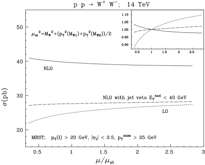
Figure 2: Scale dependence of $\sigma^{\rm cut}$, the cross section for $W$-pair production at the LHC with standard cuts. The scale is given in units of $\mu_{\rm st}$ as defined in eq. (4). We show the LO, NLO and NLO with jet veto curves without additional cuts (left) and with an additional cut $p_{T}^{\rm max}(\ell)>200$ GeV and $p_{T}^{\rm min}(\ell)>100$ GeV (right). The insets show the curves normalized to 1 at $\mu=\mu_{\rm st}$.

The purpose of these additional cuts is to investigate the scale dependence of the cross section in the region where larger corrections are expected. Indeed, the one-loop correction to the LHC cross section for $\mu=\mu_{\rm st}$ increases from 60% to 80% as the additional set of cuts is applied. Before applying the additional cuts, the situation is very similar to the Tevatron. The scale dependence at LO is reduced at NLO, and is reduced even further if the jet veto is applied. For the high $p_{T}$ case this is not quite true. The leading-order result is surprisingly stable under scale variations. This feature is somewhat artificial, however; we have checked that it does not hold if the additional cuts are changed to e.g. $p_{T}^{\rm max}(\ell)>400$ GeV and $p_{T}^{\rm min}(\ell)>200$ GeV. In this case, the leading-order cross section decreases with increasing scale. With the cuts $p_{T}^{\rm max}(\ell)>200$ GeV and $p_{T}^{\rm min}(\ell)>100$ GeV we just happen to be close to the transition from a rising to a falling leading-order cross section, a transition which is associated with the different behavior under evolution of the quark distribution functions at small $x$ vs. moderate $x$.

The reduction of the scale dependence of the next-to-leading order results when a jet veto is applied seems to be quite general though. This situation is a bit paradoxical because the cross section with a jet veto is less inclusive and, therefore, expected to be more sensitive to large logarithms created by incomplete cancellation of the infrared singularities. On the other hand, any subprocess appearing at NLO in $pp\to WW$ produces additional hadronic energy in the final state. Thus, a cut on $E_{\rm had}$ naturally suppresses the one-loop corrections and tends to stabilize the perturbative expansion. This effect competes against the stronger sensitivity to large logarithms. Apparently, for the jet veto we applied, $E_{T}^{\rm had}<40$ GeV, the subprocess-suppression effect still dominates.

3.2 $W^{+}W^{-}$

In this subsection we present some results for kinematic distributions for the processes $pp\to W^{-}W^{+}\to\ell^{-}\bar{\nu}\ell^{\prime+}\nu^{\prime}$ and $p\bar{p}\to W^{-}W^{+}\to\ell^{-}\bar{\nu}\ell^{\prime+}\nu^{\prime}$. Similar studies have been carried out earlier (see e.g. ref. [14]). Throughout, we apply our standard cuts as defined in section 2. As an illustration, we have chosen eight variables, four $p_{T}$-like quantities and four angular distributions. They all are defined in terms of observable momenta. The $p_{T}$-like distributions are defined as follows:

$p_{T}(\ell^{-})$: transverse momentum of the negatively charged lepton.

$M_{\ell\ell}$: invariant mass of the lepton pair.

$p_{T}^{\rm miss}$: missing transverse momentum, $\sqrt{(\vec{p}_{T}(\ell^{-})+\vec{p}_{T}(\ell^{\prime+})+\vec{p}_{T}({\rm jet}))^{2}}$.

$p_{T}^{\rm max}$: maximal transverse momentum of the two charged leptons, $\max\{p_{T}(\ell^{-}),p_{T}(\ell^{\prime+})\}$.

In the case of the Tevatron, the $p_{T}(\ell^{-})$ and $p_{T}(\ell^{\prime+})$ distributions are equal. However, this is not true for the LHC.

The four angular distributions we considered are defined as follows:

$\eta(\ell^{-})$: rapidity of the negatively charged lepton.

$\Delta\eta(\ell)$: rapidity difference between the leptons, $\eta(\ell^{-})-\eta(\ell^{\prime+})$.

$\cos\theta_{\ell\ell}$: angle between the leptons, $\cos(\angle[\vec{p}(\ell^{-}),\vec{p}(\ell^{\prime+})])$.

$\cos\phi_{\ell\ell}$: transverse angle between the leptons, $\cos(\angle[\vec{p}_{T}(\ell^{-}),\vec{p}_{T}(\ell^{\prime+})])$.

For massless leptons, the true rapidity $y(\ell)={1\over 2}\ln\Bigl{(}{E(\ell)+p_{L}(\ell)\over E(\ell)-p_{L}(\ell)}\Bigr{)}$ is equal to the pseudorapidity $\eta(\ell)=-\ln(\tan(\theta/2))$, so we refer to both as rapidity. For the Tevatron, we have to specify the proton direction: it corresponds to $\theta=0$.

At the Tevatron, the rapidity distribution for $\ell^{\prime+}$ can be obtained trivially from that for $\ell^{-}$ by changing the sign of $\eta$. For the LHC, there is no such simple relation between the two distributions. Note also that the $\Delta\eta(\ell)$ distribution is not symmetric around $\eta=0$ for the Tevatron; it is symmetric for the LHC. The $\cos\theta_{\ell\ell}$ observable has been investigated in ref. [27] in the context of Higgs boson detection in the intermediate Higgs mass range $m_{H}=155$–180 GeV. It is therefore particularly interesting to consider the effect of the QCD corrections to this observable.

Figure 3: Differential cross sections in pb/GeV for $W^{-}W^{+}$ production at the Tevatron for the $p_{T}$-like variables $p_{T}(\ell^{-})$, $M_{\ell\ell}$, $p_{T}^{\rm miss}$ and $p_{T}^{\rm max}$ defined in the text at LO (dashed curves) and NLO (solid curves), with $\mu=M_{W}$. Standard cuts have been applied and the branching ratios for the leptonic decay of the vector bosons are not included. The insets show the ratio $d\sigma^{NLO}/d\sigma^{LO}$. The units on the horizontal axes are GeV.

Figure 4: Differential cross sections in pb for the Tevatron for the $W^{-}W^{+}$ angular variables defined in the text at LO (dashed curves) and NLO (solid curves), with $\mu=M_{W}$. Standard cuts have been applied and the leptonic branching ratios are not included.

In Figs. 3 and 4 we show the distributions for the Tevatron, evaluated at $\mu=M_{W}$ and with our standard cuts applied. Recall that the branching ratios for the leptonic decay of the vector bosons are not included. The perturbative expansion for angular-type distributions is generally better behaved than that for steeply falling $p_{T}$-like distributions. The latter often suffer from large NLO corrections in the tails of the distribution. The insets of Fig. 3 show the ratio $d\sigma^{NLO}/d\sigma^{LO}$. They indicate that for the Tevatron, the NLO corrections are not too large, except for the $p_{T}^{\rm miss}$ distribution.

The large corrections to the $p_{T}^{\rm miss}$ distribution reflect a suppression of the Born-level cross section when $p_{T}^{\rm miss}$ is large [20]: The only way to get a large $p_{T}^{\rm miss}$ at Born level is to have a large $WW$ invariant mass. Then the two neutrinos are almost back-to-back in the $WW$ rest frame. Also, for large invariant mass the Standard Model $WW$ helicity amplitudes are dominantly those where the $W^{+}$ and $W^{-}$ have opposite helicities. The $V-A$ decay of the $W$ bosons then implies that two neutrinos tend to carry roughly the same fraction of the $W$ momentum, i.e. they have cancelling transverse momenta. NLO QCD corrections have a big effect at large $p_{T}^{\rm miss}$ because they allow a recoiling final-state parton to spoil the $p_{T}$ balance of the two neutrinos. The presence of anomalous couplings can also have a big effect in this region, by relaxing the helicity anti-correlation of the two $W$ bosons [20].

In Figs. 5 and 6, the same two sets of distributions are displayed for the LHC, again for $\mu=M_{W}$. The NLO corrections to the angular distributions are again modest. The $p_{T}$-like distributions, however, can have much larger corrections, particularly in their tails, where the NLO result can easily exceed the leading order result by a factor of 5. The $p_{T}^{\rm miss}$ distribution has the largest corrections of all, for the reason mentioned above, and the factor can be 20 or more. As mentioned before, the huge corrections in the tail of the generic $p_{T}$-like distributions have to do with the subprocess $qg\to WWq$ which dominates in this kinematical region. It may be argued that a scale choice as in eq. (4) is mandatory in this case. However, we have checked that such a scale choice does not lead to a substantial improvement.

The problem is that in a NLO calculation for $pp\to WW$ the partonic process $\bar{q}q\to WW$ is included at NLO, but the $qg\to WWq$ subprocess is included only at LO. Therefore, in a kinematical region where the latter dominates, the calculation presented in this paper is effectively only a leading order calculation. The only fully satisfactory way to improve the theoretical prediction in such cases is to include the one-loop corrections to the subprocess with a $qg$ in the initial state. These ${\cal O}(\alpha_{s}^{2})$ corrections correspond to a NNLO contribution to $pp\to WW$. At the same order in $\alpha_{s}$, there are two new subprocesses: $gg\to WW$ at one loop, and $gg\to WWq\bar{q}$ at tree level. Due to the large gluon density at small $x$, these contributions are also expected to be important for LHC energies, and would have to be included if a reliable prediction for the tails of the $p_{T}$-like distributions were required.

As discussed above, a way to suppress the partonic processes with gluons in the initial state is to impose a jet veto. The effect of the cut $E_{T}^{\rm had}>40$ GeV on the $p_{T}$-like distributions is even more dramatic than its effect on the total cross section. This can be seen in Fig. 5, where we also show the NLO curves with the jet veto (dot-dashed lines). Indeed, the one-loop corrections are very small throughout. We conclude that if a reliable theoretical prediction is desired for the tail of a $p_{T}$-like distribution, and only a next-to-leading order program is available, then a jet veto is unavoidable.

Figure 5: Differential cross sections in pb/GeV for $W^{-}W^{+}$ production at the LHC, for the $p_{T}$-like variables defined in the text at LO (dashed curves) and NLO (solid curves), with $\mu=M_{W}$. Standard cuts have been applied and the leptonic branching ratios are not included. Also shown (as dot-dashed lines) are the NLO curves with a jet veto $E_{T}^{\rm had}<40$ GeV. The insets show the ratio $d\sigma^{NLO}/d\sigma^{LO}$. The units on the horizontal axes are GeV.

Figure 6: Differential cross sections in pb for the LHC for the $W^{-}W^{+}$ angular variables defined in the text at LO (dashed curves) and NLO (solid curves), with $\mu=M_{W}$. Standard cuts have been applied and the leptonic branching ratios are not included.

3.3 $W^{\pm}Z$

In this subsection we study $WZ$ production, followed by leptonic decay of each boson. In particular, we examine the effects of QCD corrections on the approximate radiation zero at $\cos\theta=(g^{-}_{1}+g^{-}_{2})/(g^{-}_{1}-g^{-}_{2})$ [18]. Since the precise flight direction of the $W$ boson is not known, due to the uncertainty in the longitudinal momentum carried by the neutrino, we simply choose to plot a distribution in the (true) rapidity difference between the $Z$ boson and the charged lepton coming from the decay of the $W$, $\Delta y_{Z\ell}\equiv y_{Z}-y_{\ell}$. This quantity is similar to the rapidity difference $\Delta y_{WZ}\equiv|y_{W}-y_{Z}|$ studied in ref. [10], but uses only the observable charged-lepton variables. It is the direct analog of the variable $y_{\gamma}-y_{\ell^{+}}$ considered in ref. [19] for the case of $W\gamma$ production. (It is possible to determine $\cos\theta$ in the $W\gamma$ or $WZ$ rest frame, by solving for the neutrino longitudinal momentum using the $W$ mass as a constraint, up to a two-fold discrete ambiguity for each event [28]. However, ref. [19] found that the ambiguity degrades the radiation zero — at least if each solution is given a weight of 50% — so that the rapidity difference $y_{\gamma}-y_{\ell^{+}}$ is more discriminating than $\cos\theta$.)

As one can see from Fig. 7, there is a residual dip in the $\Delta y_{Z\ell}$ distribution, even at order $\alpha_{s}$. This dip can easily be enhanced by requiring a minimal energy for the decay lepton from the $W$. In Fig. 7, we have chosen $E(\ell)>100$ GeV. Note that these curves are scaled up by a factor 5. Unfortunately, only a few tens of $WZ\to$ leptons events are expected at Run II of the Tevatron, so the observation of such a dip will be rather difficult prior to the LHC.

Figure 7: For $WZ$ production at Run II, followed by leptonic decays of both the $W$ and $Z$ bosons, we plot the distribution, in picobarns, in the rapidity difference between the $Z$ and the charged lepton $\ell$ from the decay of the $W$, $\Delta y_{Z\ell}\equiv y_{Z}-y_{\ell}$. Leptonic branching ratios are not included and the scale has been set to $\mu=(M_{W}+M_{Z})/2$. The basic cuts used are $p_{T}(\ell)>20$ GeV and $|\eta(\ell)|<2$ for all three charged leptons, and a missing transverse momentum cut of $p_{T}^{\rm miss}>20$ GeV. We plot the $\Delta y_{Z\ell}$ distribution with these cuts, and also after imposing an additional cut on the $W$ decay lepton, $E(\ell)>100$ GeV; the latter curves have been scaled up by a factor of 5. The dashed curves are Born-level results; the solid curves include the ${\cal O}(\alpha_{s})$ corrections.

4 Anomalous $W^{+}W^{-}Z$ and $W^{+}W^{-}\gamma$ Couplings

4.1 Triple Gauge Boson Vertices

New physics may modify the self-interactions of vector bosons, in particular the triple gauge boson vertices. If the new physics occurs at an energy scale well above that being probed experimentally, it can be integrated out, and the result expressed as a set of anomalous (non-Standard Model) interaction vertices.

Here we consider anomalous $W^{+}W^{-}Z$ and $W^{+}W^{-}\gamma$ trilinear couplings, and their effects on the hadronic production of $WW$ and $WZ$ pairs up through order $\alpha_{s}$. The most general set of Lagrangian terms for $WWV$, $V\in\{Z,\gamma\}$, that conserves $C$ and $P$ separately, is (see e.g. [29, 30])

$${\cal L}/g_{WWV}=ig_{1}^{V}(W_{\mu\nu}^{\ast}W^{\mu}V^{\nu}-W_{\mu\nu}W^{\ast\ \mu}V^{\nu})+i\kappa^{V}W_{\mu}^{\ast}W_{\nu}V^{\mu\nu}+i\frac{\lambda^{V}}{M_{W}^{2}}W_{\rho\mu}^{\ast}W^{\mu}_{~{}\nu}V^{\nu\rho}\,,$$ (5)

where $X_{\mu\nu}\equiv\partial_{\mu}X_{\nu}-\partial_{\nu}X_{\mu}$ and the overall coupling constants $g_{WWV}$ are given by $g_{WW\gamma}=-e$ and $g_{WWZ}=-e\,\cot\theta_{W}$ respectively, with $\theta_{W}$ the weak mixing angle. The Standard Model triple gauge boson vertices are recovered by letting $g_{1}^{V}\to 1,\kappa^{V}\to 1$ and $\lambda^{V}\to 0$. The coupling factors can be written in terms of their deviation from Standard Model values: $g_{1}^{V}=1+\Delta g_{1}^{V}$ and $\kappa^{V}=1+\Delta\kappa^{V}$. Electromagnetic gauge invariance requires $g_{1}^{\gamma}=1$, or $\Delta g_{1}^{\gamma}=0$. Sometimes other constraints are imposed on the couplings. For example, if one requires the existence of an effective Lagrangian with $SU(2)\times U(1)$ invariance, and neglects operators with dimension eight or higher, then the number of independent coefficients in eq. (5) is reduced from five to three,

$$\Delta g_{1}^{Z}={\alpha_{W\phi}\over\cos^{2}\theta_{W}}\,, \hskip 56.9055pt\lambda^{\gamma}=\lambda^{Z}=\alpha_{W},$$

$$\Delta\kappa^{\gamma}=\alpha_{W\phi}+\alpha_{B\phi}\,, \hskip 56.9055pt\Delta\kappa^{Z}=\alpha_{W\phi}-{\sin^{2}\theta_{W}\over\cos^{2}\theta_{W}}\,\alpha_{B\phi},$$ (6)

where $\alpha_{W}$, $\alpha_{W\phi}$ and $\alpha_{B\phi}$ are coefficients of the dimension-six operators in this effective Lagrangian [30]. If one arbitrarily supposes that $\alpha_{W\phi}=\alpha_{B\phi}$, one arrives at the so-called HISZ scenario [31], with only two independent couplings.

The momentum-space vertex $W^{-}_{\alpha}(q)W^{+}_{\beta}({\bar{q}})V_{\mu}(p)$ (where $p+q+{\bar{q}}=0$) corresponding to eq. (5) can be written as

$$\Gamma^{\alpha\beta\mu}(q,{\bar{q}},p)/g_{WWV} = {\bar{q}}^{\alpha}g^{\beta\mu}\biggl{(}g_{1}^{V}+\kappa^{V}+\lambda^{V}{q^{2}\over M_{W}^{2}}\biggr{)}-q^{\beta}g^{\alpha\mu}\biggl{(}g_{1}^{V}+\kappa^{V}+\lambda^{V}{{\bar{q}}^{2}\over M_{W}^{2}}\biggr{)}$$ (7)

$$\hskip 28.45274pt+\bigl{(}{\bar{q}}^{\mu}-q^{\mu}\bigr{)}\Biggl{[}-g^{\alpha\beta}\biggl{(}g_{1}^{V}+{1\over 2}p^{2}\frac{\lambda^{V}}{M_{W}^{2}}\biggr{)}+\frac{\lambda^{V}}{M_{W}^{2}}p^{\alpha}p^{\beta}\Biggr{]}\,.$$

Here we have used momentum conservation, and the fact that the terms $q^{\alpha},{\bar{q}}^{\beta}$ and $p^{\mu}$ can be neglected, but we have not imposed on-shell conditions on the vector bosons. As it stands, this vertex will eventually lead to a violation of unitarity. To avoid this, the deviations from the Standard Model, $\Delta g_{1}^{V},\Delta\kappa^{V}$ and $\lambda^{V}$, have to be supplemented with form factors. Since the form factors are supposed to be produced by unknown physics, the form they should take is a priori somewhat arbitrary. We choose a conventional dipole form factor, i.e.

$$\Delta g_{1}^{V}\to{\Delta g_{1}^{V}\over(1+\hat{s}/\Lambda^{2})^{2}}\,,\qquad\Delta\kappa^{V}\to{\Delta\kappa^{V}\over(1+\hat{s}/\Lambda^{2})^{2}}\,,\qquad\lambda^{V}\to{\lambda^{V}\over(1+\hat{s}/\Lambda^{2})^{2}}\,,$$ (8)

where $\hat{s}$ is the invariant mass of the vector boson pair, and $\Lambda$ is in the TeV range.

4.2 Tree, Virtual and Bremsstrahlung Amplitudes for $WW$

Replacing the Standard Model vector-boson-vertex by the more general vertex given above results in the some modifications of the primitive amplitudes presented in ref. [15]. We use the same notation in this paper and refer the reader to ref. [15] for more details. The box-parent primitive amplitudes are not affected by changes in the trilinear vector-boson-vertex. The change in the triangle-parent primitive amplitude can be obtained by simply computing the one tree-level diagram with the new vertex. Since the vertex is no longer symmetric in the exchange $W\leftrightarrow V$, we get slightly different results for the different final states. For the $WW$ final state, the new tree amplitude, which replaces $A^{{\rm tree},b}$ in eq. (2.9) of ref. [15], is

$$A^{{\rm tree},B} = \frac{i}{2\,s_{12}\,s_{34}\,s_{56}}\Bigg{[}(g_{1}^{V}+\kappa^{V}+\lambda^{V})\bigl{(}\left\langle 1\hskip 0.42677pt3\right\rangle\left[2\hskip 0.42677pt4\right]\langle\mskip-1.0mu{6}|(1+2)|{5}\mskip-1.0mu\rangle+\left\langle 1\hskip 0.42677pt6\right\rangle\left[2\hskip 0.42677pt5\right]\langle\mskip-1.0mu{3}|(5+6)|{4}\mskip-1.0mu\rangle\bigr{)}$$ (9)

$$+ \langle\mskip-1.0mu{1}|(3+4)|{2}\mskip-1.0mu\rangle\biggl{(}2g_{1}^{V}\,\left\langle 3\hskip 0.42677pt6\right\rangle\left[4\hskip 0.42677pt5\right]+\frac{\lambda^{V}}{M_{W}^{2}}\,\langle\mskip-1.0mu{3}|(1+2)|{5}\mskip-1.0mu\rangle\langle\mskip-1.0mu{6}|(1+2)|{4}\mskip-1.0mu\rangle\biggr{)}\Bigg{]}\,.$$

For the limit $g_{1}^{V}\to 1,\kappa^{V}\to 1,\lambda^{V}\to 0$, we recover the Standard Model result,

$$A^{{\rm tree},b} = {i\over s_{12}\,s_{34}\,s_{56}}\Bigl{[}-\,\left\langle 3\hskip 0.42677pt6\right\rangle\left[4\hskip 0.42677pt5\right]\langle\mskip-1.0mu{1}|(5+6)|{2}\mskip-1.0mu\rangle+\left\langle 1\hskip 0.42677pt3\right\rangle\left[2\hskip 0.42677pt4\right]\langle\mskip-1.0mu{6}|(1+2)|{5}\mskip-1.0mu\rangle\$$ (10)

$$\qquad\qquad\ \ +\,\left\langle 1\hskip 0.42677pt6\right\rangle\left[2\hskip 0.42677pt5\right]\langle\mskip-1.0mu{3}|(5+6)|{4}\mskip-1.0mu\rangle\Bigr{]}\$$

$$= {i\over s_{12}\,s_{34}\,s_{56}}\Bigl{[}\left\langle 1\hskip 0.42677pt3\right\rangle\left[2\hskip 0.42677pt5\right]\langle\mskip-1.0mu{6}|(2+5)|{4}\mskip-1.0mu\rangle+\left[2\hskip 0.42677pt4\right]\left\langle 1\hskip 0.42677pt6\right\rangle\langle\mskip-1.0mu{3}|(1+6)|{5}\mskip-1.0mu\rangle\Bigr{]}\,.$$

With the above results we also get immediately the one-loop primitive amplitude for anomalous couplings. Assuming the usual decomposition into finite and divergent pieces, the finite pieces are vanishing, as in the Standard Model case, and the divergent pieces are still given by $c_{\Gamma}A^{{\rm tree},B}V$ where

$$V=-{1\over\epsilon^{2}}\left({\mu^{2}\over-s_{12}}\right)^{\epsilon}-{3\over 2\epsilon}\left({\mu^{2}\over-s_{12}}\right)^{\epsilon}-{7\over 2}\,.\,$$ (11)

The result for the bremsstrahlung diagrams with an additional positive helicity gluon radiated off the quark line is given by

$$A_{7}^{{\rm tree},B} = \frac{i}{2\,\left\langle 1\hskip 0.42677pt7\right\rangle\left\langle 7\hskip 0.42677pt2\right\rangle s_{34}\,s_{56}\,t_{127}}$$ (12)

$$\hskip-11.38092pt\times\Biggl{[}(g_{1}^{V}+\kappa^{V}+\lambda^{V})\bigl{(}\left\langle 1\hskip 0.42677pt3\right\rangle\langle\mskip-1.0mu{1}|(2+7)|{4}\mskip-1.0mu\rangle\langle\mskip-1.0mu{6}|(3+4)|{5}\mskip-1.0mu\rangle-\left\langle 1\hskip 0.42677pt6\right\rangle\langle\mskip-1.0mu{1}|(2+7)|{5}\mskip-1.0mu\rangle\langle\mskip-1.0mu{3}|(5+6)|{4}\mskip-1.0mu\rangle\bigr{)}$$

$$\hskip 11.38092pt+\,\langle\mskip-1.0mu{1}|(3+4)(2+7)|{1}\mskip-1.0mu\rangle\biggl{(}2g_{1}^{V}\,\left\langle 3\hskip 0.42677pt6\right\rangle\left[4\hskip 0.42677pt5\right]+\frac{\lambda^{V}}{M_{W}^{2}}\,\langle\mskip-1.0mu{3}|(4+6)|{5}\mskip-1.0mu\rangle\langle\mskip-1.0mu{6}|(3+5)|{4}\mskip-1.0mu\rangle\biggr{)}\Biggr{]}\,,$$

replacing $A_{7}^{{\rm tree},b}$ in eq. (2.22) of ref. [15]. The result for a negative helicity gluon can be obtained by the usual flip operation [15].

We also have to modify the prescription in ref. [15] for dressing the above primitive amplitudes with electroweak couplings. Since $g_{1}^{V},\kappa^{V}$ and $\lambda^{V}$ are relative couplings, i.e. the overall coupling $g_{WWV}$ has not been changed, the dressing with electroweak factors is almost identical to the Standard Model case. The only subtlety is that both $Z$ and $\gamma$ appear as intermediate states in $WW$ production. In the coefficient functions

$$C_{L,\{{u\atop d}\}} = \pm 2Q\sin^{2}\theta_{W}+{s_{12}(1\mp 2Q\sin^{2}\theta_{W})\over s_{12}-M_{Z}^{2}}\,,$$ (13)

$$C_{R,\{{u\atop d}\}} = \pm 2Q\sin^{2}\theta_{W}\mp 2Q\sin^{2}\theta_{W}\frac{s_{12}}{s_{12}-M_{Z}^{2}}\,,$$

defined in ref. [15], the first term ($\pm 2Q\sin^{2}\theta_{W}$) is from the intermediate $\gamma$, while the second term is from the intermediate $Z$. Correspondingly, we should set $V=\gamma$ ($V=Z$) in eqs. (9) and (12), when they are dressed with the first (second) term in $C_{\{{L\atop R}\},\{{u\atop d}\}}$. Otherwise, all the prefactors remain the same and only the ‘new’ primitive amplitudes have to be plugged in.

4.3 Tree, Virtual and Bremsstrahlung Amplitudes for $WZ$

For the $WZ$ final state, the new tree primitive amplitude is

$$A^{{\rm tree},B} = \frac{-i}{2\,s_{12}\,s_{34}\,s_{56}}\Bigg{[}\Bigl{(}g_{1}^{Z}+\kappa^{Z}+\lambda^{Z}\frac{s_{12}}{M_{W}^{2}}\Bigr{)}\left\langle 3\hskip 0.42677pt6\right\rangle\left[4\hskip 0.42677pt5\right]\langle\mskip-1.0mu{1}|(5+6)|{2}\mskip-1.0mu\rangle$$ (14)

$$\hskip 65.44142pt+\,(g_{1}^{Z}+\kappa^{Z}+\lambda^{Z})\left\langle 1\hskip 0.42677pt6\right\rangle\left[2\hskip 0.42677pt5\right]\langle\mskip-1.0mu{3}|(1+2)|{4}\mskip-1.0mu\rangle$$

$$\hskip 28.45274pt+\langle\mskip-1.0mu{6}|(3+4)|{5}\mskip-1.0mu\rangle\biggl{(}2g_{1}^{Z}\,\left\langle 1\hskip 0.42677pt3\right\rangle\left[2\hskip 0.42677pt4\right]+\frac{\lambda^{Z}}{M_{W}^{2}}\,\langle\mskip-1.0mu{3}|(5+6)|{2}\mskip-1.0mu\rangle\langle\mskip-1.0mu{1}|(5+6)|{4}\mskip-1.0mu\rangle\biggr{)}\Bigg{]}\,.$$

The new bremsstrahlung primitive amplitude is

$$A_{7}^{{\rm tree},B} = \frac{-i}{2\,\left\langle 1\hskip 0.42677pt7\right\rangle\left\langle 7\hskip 0.42677pt2\right\rangle s_{34}\,s_{56}\,t_{127}}$$

$$\times\Biggl{[}\Bigl{(}g_{1}^{Z}+\kappa^{Z}+\lambda^{Z}\frac{t_{127}}{M_{W}^{2}}\Bigr{)}\left\langle 3\hskip 0.42677pt6\right\rangle\left[4\hskip 0.42677pt5\right]\langle\mskip-1.0mu{1}|(5+6)(2+7)|{1}\mskip-1.0mu\rangle$$

$$\hskip 11.38092pt+\,(g_{1}^{Z}+\kappa^{Z}+\lambda^{Z})\left\langle 1\hskip 0.42677pt6\right\rangle\langle\mskip-1.0mu{1}|(2+7)|{5}\mskip-1.0mu\rangle\langle\mskip-1.0mu{3}|(5+6)|{4}\mskip-1.0mu\rangle$$

$$\hskip 11.38092pt+\,\langle\mskip-1.0mu{6}|(3+4)|{5}\mskip-1.0mu\rangle\biggl{(}-2g_{1}^{Z}\,\left\langle 1\hskip 0.42677pt3\right\rangle\langle\mskip-1.0mu{1}|(2+7)|{4}\mskip-1.0mu\rangle$$

$$\hskip 85.35826pt+\frac{\lambda^{Z}}{M_{W}^{2}}\,\langle\mskip-1.0mu{3}|(5+6)(2+7)|{1}\mskip-1.0mu\rangle\langle\mskip-1.0mu{1}|(5+6)|{4}\mskip-1.0mu\rangle\biggr{)}\Biggr{]}\,.$$

In this case, since there is only an intermediate $W$, the dressing with electroweak coupling factors is indeed identical to the Standard Model case.

4.4 Numerical Results

More systematic studies of the effects of anomalous couplings on hadronic production of vector boson pairs have been carried out elsewhere [32, 33, 34, 20, 21]. Here we merely consider one sample distribution.

The effect of anomalous couplings is enhanced for gauge bosons that are produced at large transverse momentum. In order to exploit this feature, the D0 collaboration considered a double-binned $E_{T}$ spectrum for the charged leptons coming from the decay of $W$ pairs [35]. Any deviation from the Standard Model should be more pronounced in the high $E_{T}$ bins.

$E_{T}^{\rm max}$ $\backslash$ $E_{T}^{\rm min}$	$20-38.1$	$38.1-72.5$	$72.5-138$	$138-263$	$263-500$
$\begin{array}[]{c}20-38.1\\ \left[{\rm pb}\right]\end{array}$	$\begin{array}[]{c}1.07\\ 1.07\\ 1.03\end{array}\$ 1.10	–	–	–	–
$\begin{array}[]{c}38.1-72.5\\ \left[{\rm pb}\right]\end{array}$	$\begin{array}[]{c}1.62\\ 1.62\\ 1.54\end{array}\$ 1.61	$\begin{array}[]{c}0.77\\ 0.76\\ 0.74\end{array}\$ 0.77	–	–	–
$\begin{array}[]{c}72.5-138\\ \left[10^{-1}{\rm pb}\right]\end{array}$	$\begin{array}[]{c}1.67\\ 1.60\\ 1.49\end{array}\$ 1.76	$\begin{array}[]{c}3.30\\ 3.31\\ 3.15\end{array}\$ 3.56	$\begin{array}[]{c}1.30\\ 1.32\\ 1.27\end{array}\$ 1.50	–	–
$\begin{array}[]{c}138-263\\ \left[10^{-2}{\rm pb}\right]\end{array}$	$\begin{array}[]{c}0.63\\ 0.57\\ 0.49\end{array}\$ 2.43	$\begin{array}[]{c}1.27\\ 1.20\\ 1.09\end{array}\$ 4.18	$\begin{array}[]{c}3.07\\ 3.16\\ 2.98\end{array}\$ 6.90	$\begin{array}[]{c}1.08\\ 1.14\\ 1.09\end{array}\$ 2.32	–
$\begin{array}[]{c}263-500\\ \left[10^{-4}{\rm pb}\right]\end{array}$	$\begin{array}[]{c}0.7\\ 0.6\\ 0.5\end{array}\$ 22	$\begin{array}[]{c}1.2\\ 1.1\\ 0.9\end{array}\$ 37	$\begin{array}[]{c}2.6\\ 2.5\\ 2.2\end{array}\$ 55	$\begin{array}[]{c}9.0\\ 9.8\\ 9.0\end{array}\$ 63	$\begin{array}[]{c}2.3\\ 2.5\\ 2.4\end{array}\$ 9.5

Table 3: Double-binned $E_{T}$ cross sections for $p\bar{p}\to W^{+}W^{-}\to$ leptons at $\sqrt{s}=2$ TeV. The three numbers in the left column in each entry are the Standard Model results for the scales $\mu=\mu_{\rm st}\times\{1/2,1,2\}$, with $\mu_{\rm st}$ given in eq. (4). The fourth number in the entry is the cross section with anomalous couplings, as defined in the text.

We have computed a similar double-binned $E_{T}$ spectrum at NLO for Run II of the Tevatron. As in ref. [35] we compute for each event the larger and smaller transverse energies of the two leptons, $E_{T}^{\rm max}$ and $E_{T}^{\rm min}$. ($E_{T}$ is equivalent to $p_{T}(\ell)$, of course.) We impose our standard event cuts and then bin each $E_{T}$ into five bins with the following limits in GeV:

$$E_{T}=\{20,38.1,72.5,138,263,500\}.$$ (16)

In order to get a feeling for the theoretical uncertainties, we repeated the Standard Model computation for three scales, $\mu_{\rm st}/2$, $\mu_{\rm st}$ and $2\mu_{\rm st}$, where $\mu_{\rm st}$ is given in eq. (4). We computed the same NLO double-binned cross section including the effects of anomalous couplings. As an illustration we have chosen the HISZ scenario with $\alpha_{W}=\alpha_{W\phi}=\alpha_{B\phi}=0.1$. This corresponds to the following values for the anomalous couplings appearing in the Lagrangian in eq. (5):

$$\Delta g_{1}^{\gamma}=0;\ \ \Delta g_{1}^{Z}=0.13;\ \ \lambda^{\gamma}=\lambda^{Z}=0.1;\ \ \Delta\kappa^{\gamma}=0.2;\ \ \Delta\kappa^{Z}=0.07.$$ (17)

The form factors have been chosen according to eq. (8) with $\Lambda=2$ TeV. At present these values are still consistent with LEP2 bounds [36]. Table 3 presents the results. As usual, the leptonic branching ratios are not included, and we use the MRST parton distributions. The three numbers in the left column of each box give the Standard Model result for the three choices of $\mu$, with $\mu$ increasing from top to bottom. The fourth number in each box is the result with the anomalous couplings included and $\mu=\mu_{\rm st}$. Units for the cross sections for each row are given in square brackets. As expected, the results for the Standard Model and anomalous cross section are very similar for the low $E_{T}$ bins. For the high $E_{T}$ bins, however, the differences are large and certainly much bigger than the most conservative estimate of the theoretical error.

The same results are also shown in Fig. 8, where we plot the natural logarithm of the total cross section (in units of $10^{-1}$ fb) for each bin for the Standard Model with $\mu=\mu_{\rm st}$ (left) and the HISZ scenario with $\mu=\mu_{\rm st}$ (right). Again, the significant differences in the high $E_{T}$ bins become apparent.

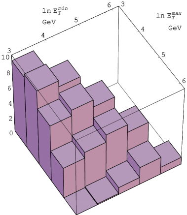
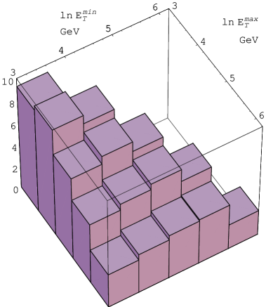
Figure 8: Cross section $\sigma$ [fb/10] for $W$-pair production at the Tevatron with no anomalous couplings (left) and for the HISZ scenario with $\alpha_{W}=\alpha_{W\phi}=\alpha_{B\phi}=0.1$ (right). Standard cuts have been applied and the scale has been set to $\mu=\mu_{\rm st}$ as defined in eq. (4).

5 Conclusions

We have presented a general purpose Monte Carlo program that is able to compute any infrared-safe quantity in vector boson pair production at hadron colliders at next-to-leading order in the strong coupling constant $\alpha_{s}$. This program generalizes previous calculations (with the exception of the recent ref. [17]) in that the spin correlations are fully taken into account. The decay of the vector bosons into leptons was included in the narrow-width approximation, whereas MCFM [17] also includes the singly-resonant diagrams needed to go beyond this approximation. For the total cross-section, computed in the narrow-width approximation, our results agree perfectly with those of MCFM for the same choice of input parameters.

As an illustration of the usefulness of the program we presented several distributions for the Run II at the Tevatron and the LHC. However, we refrained from performing a detailed phenomenological analysis; this is probably best done once the data are available.

In addition to Standard Model processes, we considered also the inclusion of anomalous couplings between the vector bosons. We presented the one-loop amplitudes for a generalized trilinear $W^{+}W^{-}Z$ and $W^{+}W^{-}\gamma$ vertex. The inclusion of these amplitudes into our program allows the calculation of anomalous effects at next-to-leading order, with full spin correlations. These effects are shown to be very prominent for large transverse momentum of the gauge bosons, confirming results of ref. [20]. Such an analysis at Run II of the Tevatron should yield improved bounds on anomalous couplings, although for large improvements one probably has to wait for the LHC [30].

Acknowledgments

L.D. and A.S. would like to thank the Theory Group of ETH Zürich for its hospitality while part of this work was carried out. We are grateful to John Campbell and Keith Ellis for assistance in the comparison of our results with those of ref. [17].

References

- [1] E. Eichten, I. Hinchliffe, K. Lane and C. Quigg, Rev. Mod. Phys. 56 (1984) 579.
-
[2]
A.A. Iogansen, N.G. Ural’tsev and V.A. Khoze, Sov. J. Nucl. Phys.
36 (1983) 717;
J.F. Gunion, H.E. Haber, G. Kane and S. Dawson, The Higgs Hunter’s Guide (Addison-Wesley, 1990). - [3] M.S. Chanowitz and W.B. Kilgore, Phys. Lett. B347 (1995) 387 [hep-ph/9412275].
-
[4]
K.T. Matchev and D.M. Pierce, preprint hep-ph/9904282;
H. Baer, et al., preprint hep-ph/9906233. -
[5]
F. Abe, et al. (CDF Collaboration), Phys. Rev. Lett. 75 (1995) 1017;
S. Abachi, et al. (D0 Collaboration), Phys. Rev. Lett. 77 (1996) 3303;
S. Abachi, et al. (D0 Collaboration), Phys. Rev. Lett. 79 (1997) 1441. -
[6]
R.W. Brown and K.O. Mikaelian, Phys. Rev. D19 (1979) 922;
R.W. Brown, K.O. Mikaelian and D. Sahdev, Phys. Rev. D20 (1979) 1164;
K.O. Mikaelian, M.A. Samuel and D. Sahdev, Phys. Rev. Lett. 43 (1979) 746. - [7] J. Ohnemus, Phys. Rev. D44 (1991) 1403.
- [8] S. Frixione, Nucl. Phys. B410 (1993) 280.
- [9] J. Ohnemus, Phys. Rev. D44 (1991) 3477.
- [10] S. Frixione, P. Nason and G. Ridolfi, Nucl. Phys. B383 (1992) 3.
- [11] J. Ohnemus and J.F. Owens, Phys. Rev. D43 (1991) 3626.
- [12] B. Mele, P. Nason and G. Ridolfi, Nucl. Phys. B357 (1991) 409.
- [13] J.F. Gunion and Z. Kunszt, Phys. Rev. D33 (1986) 665.
- [14] J. Ohnemus, Phys. Rev. D50 (1994) 1931 [hep-ph/9403331].
- [15] L. Dixon, Z. Kunszt and A. Signer, Nucl. Phys. B531 (1998) 3 [hep-ph/9803250].
- [16] S. Frixione, Z. Kunszt and A. Signer, Nucl. Phys. B467 (1996) 399 [hep-ph/9512328].
- [17] J.M. Campbell and R.K. Ellis, preprint hep-ph/9905386.
- [18] U. Baur, T. Han and J. Ohnemus, Phys. Rev. Lett. 72 (1994) 3941 [hep-ph/9403248].
- [19] U. Baur, S. Errede and G. Landsberg, Phys. Rev. D50 (1994) 1917 [hep-ph/9402282].
- [20] U. Baur, T. Han and J. Ohnemus, Phys. Rev. D53 (1996) 1098 [hep-ph/9507336].
- [21] U. Baur, T. Han and J. Ohnemus, Phys. Rev. D51 (1995) 3381 [hep-ph/9410266].
- [22] R.K. Ellis, D.A. Ross and A.E. Terrano, Nucl. Phys. B178 (1981) 421.
- [23] A.D. Martin, R.G. Roberts, W.J. Stirling and R.S. Thorne, Eur. Phys. J C4 (1998) 463 [hep-ph/9803445].
- [24] H.L. Lai et al. (CTEQ collaboration), Phys. Rev. D55 (1997) 1280 [hep-ph/9606399].
- [25] S. Dittmaier, M. Bohm and A. Denner, Nucl. Phys. B376 (1992) 29, err. B391 (1993) 483.
- [26] W. Beenakker et al., in Physics at LEP2, eds. G. Altarelli, T. Sjöstrand and F. Zwirner (Geneva, 1996).
- [27] M. Dittmar and H. Dreiner, Phys. Rev. D55 (1997) 167 [hep-ph/9608317]; hep-ph/9703401, in Tegernsee 1996, The Higgs Puzzle.
-
[28]
J. Gunion, Z. Kunszt and M. Soldate, Phys. Lett. 163B (1985) 389;
J. Gunion and M. Soldate, Phys. Rev. D34 (1986) 826;
W.J. Stirling et al., Phys. Lett. 163B (1985) 261. - [29] K. Hagiwara, R.D. Peccei, D. Zeppenfeld and K. Hikasa, Nucl. Phys. B282 (1987) 253.
- [30] J. Ellison and J. Wudka, preprint hep-ph/9804322, to appear in Ann. Rev. Nucl. Part. Sci.
- [31] K. Hagiwara, S. Ishihara, R. Szalapski and D. Zeppenfeld, Phys. Rev. D48 (1993) 2182.
- [32] U. Baur and D. Zeppenfeld, Nucl. Phys. B308 (1988) 127.
- [33] U. Baur, T. Han and J. Ohnemus, Phys. Rev. D48 (1993) 5140 [hep-ph/9305314].
- [34] U. Baur, T. Han and J. Ohnemus, Phys. Rev. D57 (1998) 2823 [hep-ph/9710416].
- [35] B. Abbott et al. (D0 collaboration) Phys. Rev. D58 (1998) 051101 [hep-ex/9803004].
- [36] LEP Collaborations, LEP Electroweak Working Group, and SLD Heavy Flavour and Electroweak Groups, preprint CERN-EP/99-15 (February, 1999).