Angular Dependence of the Radiative Gluon Spectrum
and the Energy Loss of Hard Jets in QCD Media

Abstract

The induced momentum spectrum of soft gluons radiated from a high energy quark propagating through a QCD medium is derived in the BDMPS formalism. A calorimetric measurement for the medium dependent energy lost by a jet with opening angle $\theta_{{\rm cone}}$ is proposed.The fraction of this energy loss with respect to the integrated one appears to be the relevant observable.It exhibits a universal behaviour in terms of the variable $\theta^{2}_{{\rm cone}}L^{3}\hat{q}$ where $L$ is the size of the medium and $\hat{q}$ the transport coefficient. Phenomenological implications for the differences between cold and hot QCD matter are discussed.

I Introduction

The medium induced energy loss of a hard (quark or gluon) jet traversing matter - hot or cold - has recently been the subject of intensive interest [1, 2, 3, 4, 5, 6, 7, 8, 9, 10, 11, 12, 13, 14]. The radiative energy loss has been found to be independent of the jet energy, for large energies, and growing as $L^{2}$ where $L$ is the extent of the medium [4, 5]. The order of magnitude of this effect in hot matter may be expected to be large enough - compared to the case of cold nuclear matter - to lead to an observable and remarkable signal of the production of deconfined matter.

The natural observable to measure this energy loss would then be the transverse momentum spectrum of hard jets produced in heavy-ion collisions. Jet quenching which has been discussed recently in [15, 16] is the manifestation of energy loss as seen in the suppression and change of shape of the jet spectrum compared with hadronic data. One may also think of measuring single particle inclusive spectra. Comparisons of high $p_{\bot}$ particle spectra in $p+p,p+A$ and $A+B$ collisions at SPS energies have already been performed and discussed [15]. The results seem to be difficult to interpret in view of the obvious model dependence of the theoretical prediction. This model dependence is associated with the relatively low energy and $p_{\bot}$ ranges which are currently accessible [16]. The situation should be much more favorable at RHIC. Jet production will be intensively studied at LHC.

In Section 2 of the present paper we study the angular distribution of radiated gluons which are believed to be the main source of energy loss. This allows for quantitative predictions of the energy lost outside the cone defining the jet. This problem has already been considered in [9, 10, 11], where the expression of the “characteristic” angle for gluon emission has been worked out. We work along the same lines but we perform a more complete calculation of the angular distribution. We concentrate on the realistic case of a hard jet produced in the medium. We make the implicit assumption that the lifetime of the hot medium is large enough to allow for a large number of scatterings of the jet as it traverses the medium.

In Section 3 we calculate the integrated energy loss outside an angular cone with fixed opening angle, $\Delta E(\theta_{{\rm cone}})$, and derive the expression for the ratio $R(\theta_{{\rm cone}})={\Delta E(\theta_{{\rm cone}})/\Delta E}$, where $\Delta E$ is the completely integrated loss. For simplicity of expression we take a convention where $\Delta E$ is a positive quantity. The surprising result is that $R(\theta_{{\rm cone}})$ is a universal function of the variable $\theta^{2}_{{\rm cone}}\hat{q}L^{3}$, where $\hat{q}$ is the transport coefficient characteristic of the medium.

In Section 4 we give estimates and in particular we show that the energy loss is more collimated in the case of a hot QCD medium as compared to nuclear matter. As a consequence the characteristic angle for gluon emission in a hot medium is quite small of the order of $10^{\circ}$ for a temperature of 250 MeV. It is, however, possible to choose large enough angles of the order of $30^{\circ}$ and still have an appreciable energy loss. We also make a comparison with the corresponding energy loss outside a cone in the vacuum. All the calculations are done on the partonic level with no attempt to include fragmentation of partons into hadrons. Fragmentation effects, as well as effects due to plasma expansion [14], could be important and should be studied.

Technical details are summarized in Appendices A - C.

II Momentum spectrum of radiated gluons

In this section we discuss the induced momentum spectrum of soft gluon emission $(x\rightarrow 0)$ from a fast quark jet. We assume that the quark is produced inside the medium by a hard scattering at time $t=0$. From the production point it propagates over a length $L$ of QCD matter, carrying out many scatterings with the medium. We follow closely the derivation and notation given in BDMPS [4, 5] (denoted by I and II) and BDMS [6] which we denote by III.

In the case under consideration the spectrum per unit length $z$ of the medium consists of two terms: one corresponding to an “on-shell” quark, as if that quark were entering the medium, and one corresponding to a hard production vertex as described in III (cf. Eq.(31)):

$$\frac{\omega dI}{d\omega dzd^{2}\underline{U}}=\frac{\omega dI}{d\omega dzd^{2}\underline{U}}\,\,\Bigg{|}_{{\rm on-shell}}+\frac{\omega dI}{d\omega dzd^{2}\underline{U}}\,\,\Bigg{|}_{{\rm vertex}}.$$ (1)

$\omega$ denotes the soft gluon energy and $\underline{U}$ the scaled transverse gluon momentum $\underline{U}=\underline{k}/\mu$ with $\mu$ the appropriate scale of the QCD potential.

As follows from Eq.(31) in III the induced gluon spectrum is

$$\frac{\omega dI}{d\omega dzd^{2}\underline{U}} = \frac{\alpha_{s}C_{F}}{\pi^{2}L}2\,Re\,\int^{L}_{0}\,dt_{2}\int d^{2}\underline{Q}\left\{\int^{t_{2}}_{0}\,dt_{1}\rho\sigma\frac{N_{c}}{2C_{F}}f(\underline{U}+\underline{Q},t_{2}-t_{1})+f_{h}(\underline{U}+\underline{Q},t_{2})\right\}$$ (2)

$$\times \rho\sigma\frac{N_{c}}{2C_{F}}2\left[\frac{\underline{U}+\underline{Q}}{(\underline{U}+\underline{Q})^{2}}-\frac{\underline{U}}{\underline{U}^{2}}\right]V(\underline{Q})\,{\cal F}_{fsi}\,\Bigg{|}^{\tilde{\kappa}=0}_{\tilde{\kappa}},$$ (3)

where $f_{h}$ differs from $f$ in that the gluon emission time has been evaluated at the time of the hard interaction, $t=0$. After we have converted (2) to impact parameter space the explicit relationship between $f_{h}$ and $f$ will be given. In the soft $\omega$ limit the contributions from the diagrams (Fig. 1a-c) are included. In comparison with the diagrams shown in Fig. 4 of III we note that the soft limit leads to a vanishing of the sum of diagrams Fig. 4d-4j.

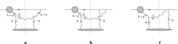
FIG. 1.: The diagrams representing the contributions to the spectrum (2).

The quantities in (2), explained in III, have the following meaning: $\alpha_{s}C_{F}/\pi^{2}$ is the coupling of a gluon to a quark. The factor $\frac{N_{c}}{2C_{F}}f(\underline{U}+\underline{Q},t_{2}-t_{1})\rho\sigma dt_{1}$ gives the number of scatterers in the medium, $\rho\sigma dt_{1}$, times the gluon emission amplitude at $t_{1}$, evolved to $t_{2}$. The momentum labels are shown in Fig. 1. We describe the scattering in terms of the normalized cross section $V(\underline{Q})=\frac{1}{\pi\sigma}\frac{d\sigma}{d\underline{Q}^{2}}$ which depends on the scaled momentum $\underline{Q}={\underline{q}}/{\mu}$. We note that the final state gluon carries a transverse momentum $\underline{k}$. The factor corresponding to the amplitude $f_{0}^{\star}$ in III which sums the gluon emissions (Fig. 1a-c) is $\int d^{2}\underline{Q}\,V(\underline{Q})\,2\left[\frac{\underline{U}+\underline{Q}}{(\underline{U}+\underline{Q})^{2}}-\frac{\underline{U}}{\underline{U}^{2}}\right]$. In order to eliminate the medium-independent factorisation contribution one has to perform a subtraction of the value of the integrals at $\tilde{\kappa}=0$ [3, 4, 5, 6]. The parameter $\tilde{\kappa}$

$$\tilde{\kappa}=\frac{2C_{F}}{N_{c}}\frac{\lambda\mu^{2}}{2\omega},$$ (4)

depends on medium properties, in particular on the quark’s mean free path $\lambda=1/\rho\sigma$, as well as on the gluon energy.

In dealing with (2) in contrast to the $\underline{U}$-integrated spectrum discussed in III we now have to take into account the possibility that the emitted gluon may rescatter in the medium. For example the contribution shown in Fig. 1a may now have final state interactions as illustrated in Fig. 2.

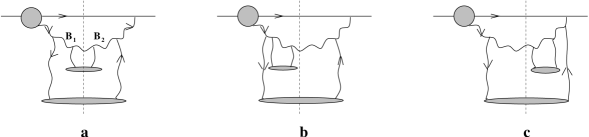
FIG. 2.: Final state interactions contributing to Fig. 1a: (a) real, (b) and (c) virtual interactions.

This is taken care of by the final state interaction amplitude ${\cal F}_{fsi}$ in (2) which is most conveniently expressed in impact parameter space. One goes to impact parameter space by taking the Fourier transform, for example for the amplitude $f(\underline{U},t)$,

$$f(\underline{U},t)=\int\,\frac{d^{2}\underline{B}}{(2\pi)^{2}}\,e^{i\underline{B}\cdot\underline{U}}\tilde{f}(\underline{B},t).$$ (5)

As in III we rescale the time variable $t=\frac{2C_{F}}{N_{c}}\lambda\tau$ and define

$$\tau_{0}=N_{c}L/2C_{F}\lambda.$$ (6)

Following our analysis of parton $p_{\bot}$-broadening in II we write the final state interaction amplitude as

$${\cal F}_{fsi}(\underline{B}_{1}-\underline{B}_{2},\tau)=\exp\,\left[-\frac{1}{2}(\underline{B}_{1}-\underline{B}_{2})^{2}\tau\tilde{v}\right].$$ (7)

In II the distribution in transverse momentum and the corresponding distribution in impact parameter were given for a single parton going through a medium. Here we have a quark-gluon system passing through the medium. However, interactions of the quark with the medium cancel between real and virtual interactions leaving only the interactions of the gluon with the medium as in II. These interactions can be real interactions, as shown in Fig. 2a where both the gluon in the amplitude at impact parameter $\underline{B}_{1}$ and in the complex conjugate amplitude at $\underline{B}_{2}$ interact with the medium, or they can be virtual interactions as shown in Figs. 2b and 2c. The real interactions give a factor $\tilde{V}(\underline{B}_{1}-\underline{B}_{2})$ while the virtual interactions give the absorption of the gluon wave and a factor of $-\tilde{V}(0)=-1$. $\tilde{V}(\underline{B})$ is the Fourier transform of the potential $V(\underline{Q})$. These terms combine together giving at small $\underline{B}_{1}-\underline{B}_{2}$

$$1-\tilde{V}(\underline{B}_{1}-\underline{B}_{2})\simeq\frac{1}{4}(\underline{B}_{1}-\underline{B}_{2})^{2}\,\tilde{v}.$$ (8)

$\tilde{v}$ has a logarithmic dependence on $\underline{B}^{2}$. In the following we neglect the variation of the logarithm, an approximation which is good except when large transverse momentum rescatterings occur (see II). The factor in (8) then exponentiates, as in II, to give (7), where the $\frac{1}{2}$ in the exponent (7) differs from the $\frac{1}{4}$ in Eq.(27) of II because of the difference of $\tau$ from $t$ used there. Using (5) and (7) in (2) we obtain the spectrum in terms of impact parameter integrals,

$$\frac{\omega dI}{d\omega dzd^{2}\underline{U}} = \frac{\alpha_{s}C_{F}}{\pi^{2}L}2Re\,\int^{\tau_{0}}_{0}\,d\tau_{2}\,\int\,\frac{d^{2}B_{1}}{(2\pi)^{2}}\frac{d^{2}B_{2}}{(2\pi)^{2}}\,e^{i(\underline{B}_{1}-\underline{B}_{2})\cdot\underline{U}}\,\left\{\int^{\tau_{2}}_{0}\,d\tau_{1}\tilde{f}(\underline{B}_{1},\tau_{2}-\tau_{1})+\frac{2}{\tilde{v}\underline{B}_{1}^{2}}\tilde{f}(\underline{B}_{1},\tau_{2})\right\}$$ (9)

$$\times \frac{4\pi i\underline{B}_{2}}{\underline{B}_{2}^{2}}\left[\tilde{V}(\underline{B}_{1}-\underline{B}_{2})-\tilde{V}(\underline{B}_{1})\right]e^{-\frac{\tilde{v}}{2}(\underline{B}_{1}-\underline{B}_{2})^{2}(\tau_{0}-\tau_{2})}\Bigg{|}^{\tilde{\kappa}=0}_{\tilde{\kappa}}.$$ (10)

We have used $\tilde{f}_{h}(\underline{B},\tau)=\frac{2}{\tilde{v}\underline{B}^{2}}\tilde{f}(\underline{B},\tau)$ which follows from the fact that $\tilde{f}_{h}$ and $\tilde{f}$ have the same time evolution while the initial conditions satisfy $\tilde{f}_{h}(\underline{B},0)=\frac{2}{\tilde{v}\underline{B}^{2}}\tilde{f}(\underline{B},0)$ as can be seen by comparing Eqs.(16) and (17b) of III in the soft gluon limit.

When integrating (9) with respect to the gluon momentum $\underline{U}$ it is straightforward to reproduce the energy spectrum given e.g. in Eq.(34) of III. Next we recall that the amplitude $\tilde{f}(\underline{B},\tau)$ is given by (cf. Eq.(38) in III)

$$\tilde{f}(\underline{B},\tau)=-\frac{i\pi\tilde{v}}{\cos^{2}\omega_{0}\tau}\underline{B}\exp\left(-\frac{i}{2}m\omega_{0}\underline{B}^{2}\tan\omega_{0}\tau\right),$$ (11)

with

$$m=-1/2\tilde{\kappa}\,\,\,{\rm and}\,\,\,\omega_{0}=\sqrt{2i\tilde{\kappa}\tilde{v}},$$ (12)

together with $\tilde{\kappa}$ given in (4). In this approximation (leading logarithm and small $x$) after substituting (11) into (9) we find a convenient expression for the momentum spectrum per unit length

$$\frac{\omega dI}{d\omega dzd^{2}\underline{U}}=\frac{2\alpha_{s}C_{F}}{L}\tilde{v}^{2}Re\,\int^{\tau_{0}}_{0}\,\frac{d\tau}{\cos^{2}\omega_{0}\tau}\,\left\{\int^{\tau_{0}-\tau}_{0}\,d\tau_{1}\,I(\underline{U},\alpha,\beta)+\int^{\tau_{0}-\tau}_{-\infty}\,d\tau_{1}\,I(\underline{U},\alpha+\beta,\beta^{\prime})\right\}\Bigg{|}^{\tilde{\kappa}=0}_{\tilde{\kappa}},$$ (13)

with the time dependent variables

$$\alpha = \frac{i}{2}m\omega_{0}\tan\omega_{0}\tau=\frac{\tilde{v}}{2}\frac{\tan\omega_{0}\tau}{\omega_{0}},$$ (14)

$$\beta = \frac{\tilde{v}}{2}(\tau_{0}-\tau-\tau_{1}),$$ (15)

$$\beta^{\prime} = \frac{\tilde{v}}{2}(\tau_{0}-\tau).$$ (16)

After using (8) in (9) the $\underline{B}$-space integrals become

$$I(\underline{U},\alpha,\beta) = \int\,\frac{d^{2}\underline{B}_{1}}{(2\pi)^{2}}\,\frac{d^{2}\underline{B}_{2}}{(2\pi)^{2}}\,e^{i(\underline{B}_{1}-\underline{B}_{2})\cdot\underline{U}}$$ (17)

$$\times \frac{\underline{B}_{2}\cdot\underline{B}_{1}}{\underline{B}_{2}^{2}}\left[\underline{B}_{1}^{2}-(\underline{B}_{1}-\underline{B}_{2})^{2}\right]\exp\left[-\alpha\underline{B}_{1}^{2}-\beta(\underline{B}_{1}-\underline{B}_{2})^{2}\right].$$ (18)

It is evaluated in Appendix A with the explicit result (A13),

$$I(\underline{U},\alpha,\beta)=\frac{1}{16\pi}\,\frac{1}{\alpha^{2}(\alpha+\beta)}e^{-\frac{\underline{U}^{2}}{4(\alpha+\beta)}}.$$ (19)

From the induced momentum spectrum (13), (14) one may rederive the $\omega$-spectrum per unit length $\omega dI/d\omega dz$ for soft gluon emission off quark jets produced inside the medium. After performing the exponential $\underline{U}$-integration and the $\tau,\tau_{1}$ integrals explicitly the result of III is reproduced, namely

$$\frac{\omega dI}{d\omega dz}=\frac{2\alpha_{s}C_{F}}{\pi L}\,\ln|\cos\omega_{0}\tau_{0}|.$$ (20)

We note from (6) and (12) that $\omega_{0}\tau_{0}$ is expressed in terms of medium-dependent quantities and the gluon energy $\omega$ by

$$(\omega_{0}\tau_{0})^{2} = i\frac{N_{c}}{2C_{F}}\,\frac{\mu^{2}\tilde{v}}{\lambda}\,L^{2}/\omega$$ (21)

$$= i\frac{N_{c}}{2C_{F}}\,\hat{q}L^{2}/\omega,$$ (22)

where we introduce the transport coefficient [4, 5]

$$\hat{q}\equiv\frac{\mu^{2}\tilde{v}}{\lambda}=\rho\,\int^{1/\underline{B}^{2}}_{0}\,d\underline{Q}^{2}\,\underline{Q}^{2}\,\frac{d\sigma}{d\underline{Q}^{2}}.$$ (23)

Integrating (20) over $\omega$ the energy loss per unit length is obtained as

$$-dE/dz=\int^{\infty}_{0}\,\frac{\omega dI}{d\omega dz}\,d\omega=\frac{\alpha_{s}N_{C}}{4}\,\hat{q}L,$$ (24)

so long as $E>E_{cr}\simeq\hat{q}L^{2}$ [4].

III Induced radiative energy loss of a hard quark jet in a finite cone

Let us consider a typical calorimetric measurement. We have in mind a hard quark jet of high energy $E$ produced by a hard scattering in a dense QCD medium and propagating through it over a distance $L$. The quark loses energy by gluon radiation induced by multiple scattering. In the following we calculate the integrated loss outside an angular cone of opening angle $\theta_{{\rm cone}}$ (Fig. 3),

$$\Delta E(\theta_{{\rm cone}})=L\,\int^{\infty}_{0}\,d\omega\,\int^{\pi}_{\theta_{{\rm cone}}}\,\frac{\omega dI}{d\omega dzd\theta}d\theta.$$ (25)

FIG. 3.: Hard process producing a quark jet. The gluon is emitted outside the cone with angle $\theta_{{\rm cone}}$.

We note that for $\theta_{{\rm cone}}=0$ the total loss (24) is obtained, namely [6]

$$\Delta E=\frac{\alpha_{s}N_{c}}{4}\hat{q}L^{2}.$$ (26)

In detail we consider the normalized loss by defining the ratio

$$R(\theta_{{\rm cone}})=\frac{\Delta E(\theta_{{\rm cone}})}{\Delta E},$$ (27)

which may be decomposed into

$$R(\theta_{{\rm cone}})=R_{{\rm on-shell}}(\theta_{{\rm cone}})+R_{{\rm vertex}}(\theta_{{\rm cone}})$$ (28)

according to the treatment in the previous section.

Defining ${\underline{U}^{2}_{{\rm cone}}}$ in the approximation of small cone angles

$$\underline{U}^{2}_{\rm cone}\simeq\frac{\omega^{2}}{\mu^{2}}\theta^{2}_{\rm cone},$$ (29)

the $\theta$ integral in (25) may be performed using

$$\int^{\infty}_{\underline{U}^{2}_{{\rm cone}}}\,d^{2}\underline{U}\,I(\underline{U},\alpha,\beta)=\frac{1}{4\pi\alpha^{2}}\exp\left[{-\frac{\omega^{2}\theta^{2}_{{\rm cone}}}{4\mu^{2}(\alpha+\beta)}}\right].$$ (30)

The remaining $\omega,\tau$ and $\tau_{1}$ integrations cannot be done analytically. It is convenient to change variables by introducing dimensionless ones:

$$\tau \equiv \tau_{0}y,$$ (31)

$$\tau_{1} \equiv \tau_{0}z,$$ (32)

$$\omega_{0}\tau \equiv (1+i)x,$$ (33)

which implies that the gluon energy is expressed by

$$\omega=\frac{C_{F}}{N_{c}}\lambda\mu^{2}\tilde{v}\tau^{2}_{0}(y/x)^{2}.$$ (34)

As a nice consequence, the ratio $R(\theta_{{\rm cone}})$ turns out to depend on one single dimensionless variable

$$R=R(c(L)\theta_{{\rm cone}}),$$ (35)

where

$$c^{2}(L)=\frac{N_{c}}{2C_{F}}\hat{q}\left(L/2\right)^{3}.$$ (36)

The “scaling behaviour” of $R$ means that the medium and size dependence is universally contained in the function $c(L)$, which is a function of the transport coefficient $\hat{q}$ (23) and of the length $L$, as defined by (36). For fixed $L$ the medium properties are exclusively described by $\hat{q}$ which is different for cold and hot matter (cf. our discussion in Sect. 5 of II). The fact that $\theta_{{\rm cone}}$ scales as $1/c(L)$ may be understood from the following physical argument [9]: the radiative energy loss of a quark jet is dominated by gluons having $\omega\simeq\hat{q}L^{2}$ (cf. Eq.(6.9) in I). The angle that the emitted gluon makes with the quark is $\theta={\underline{k}}/{\omega}$ with $\underline{k}$ the gluon transverse momentum. But $\underline{k}^{2}\simeq\hat{q}L$ so that the typical gluon angle will be $\theta^{2}\simeq\frac{1}{\hat{q}L^{3}}$ or $\theta^{2}\simeq\left[\frac{(\hat{q})^{1/3}}{\omega}\right]^{3/2}$.

FIG. 4.: Fractional induced loss $R(\theta_{{\rm cone}})$ (solid curve) as a function of $c(L)\theta_{{\rm cone}}$, and decomposed into $R_{{\rm on-shell}}$ (dashed curve) and $R_{{\rm vertex}}$ (dotted curve).

For completeness the explicit dependence of $R$ on $c(L)\theta_{{\rm cone}}$ is given in Appendix B. The numerical evaluation of this dependence is shown in Fig. 4 [17]. The following remarks may be useful. Obviously by definition $R(\theta_{{\rm cone}}=0)=1$, where we know from III that

$$R_{{\rm on-shell}}(\theta_{{\rm cone}}=0)=1/3\,\,\,\,\,\,{\rm and}\,\,\,\,\,\,R_{{\rm vertex}}(\theta_{{\rm cone}}=0)=2/3.$$ (37)

At large angles, $c(L)\theta_{{\rm cone}}\gg 1$, we find (see Appendix C) the power behaviour

$$R(\theta_{{\rm cone}})\longrightarrow\frac{4\Gamma(1/4)}{5\pi}\frac{1}{(c(L)\theta_{{\rm cone}})^{1/2}},$$ (38)

coming exclusively from $R_{{\rm on-shell}}$. $R_{{\rm vertex}}(\theta_{{\rm cone}})$ vanishes faster than the dependence given in (38), as may be seen from (C9).

The ratio $R(\theta_{{\rm cone}})$ is also universal in the sense that it is the same for an energetic quark as well as for a gluon jet, since the function $c(L)$ depends on the product $C_{F}\lambda=N_{c}\lambda_{gluon}$( $=C_{R}\lambda_{R}$ for colour representation R). It is the integrated loss, however, which is bigger by the factor $N_{c}/C_{F}$ for the gluon than for the quark jet.

The “narrowness” of the angular distribution can be read off from Fig. 4: e.g. $R(\theta_{{\rm cone}})$ decreases from $1$ to $0.4$, when $c(L)\theta_{{\rm cone}}$ is increased from zero to $10$. Explicit values for $c(L)$ are discussed in Sect. 4 when comparing hot and cold QCD matter for fixed $L$

$$c(L)\Big{|}_{{\rm HOT}}\gg c(L)\big{|}_{{\rm COLD}},$$ (39)

so that $R(\theta_{{\rm cone}})\Big{|}_{{\rm HOT}}$ is much narrower than $R(\theta_{{\rm cone}})\Big{|}_{{\rm COLD}}$ when considered as a function of $\theta_{{\rm cone}}$.

IV Phenomenology

We know from I - III that the transport coefficient $\hat{q}$ (23) controls the medium induced energy loss (26) as well as the $p_{\bot}$-broadening of high energy partons: both quantities are directly proportional to $\hat{q}$. The medium dependence of the distribution $R(\theta_{{\rm cone}})$ in (35) (see also Appendix B) is determined by the coefficient $c(L)$ which according to (36) depends on the square root of $\hat{q}$. In this section we estimate the magnitude of $c(L)$, with the aim of finding differences in the angular distributions $R(\theta_{{\rm cone}})$ for cold and hot matter. In the following we will confirm the statement given in (39) quantitatively. In order to be able to compare with our discussion already given in II (and in III) we keep the same numerical values for the quantity $\hat{q}$ as used there.

(i) For hot matter at reference temperature $T=250$ MeV we take

$$\hat{q}\simeq 0.1\,{\rm GeV}^{3}.$$ (40)

This value is deduced from (23) using the screened one-gluon exchange cross section, e.g. for two flavours one derives [2]

$$\hat{q}\simeq\frac{48}{\pi}\zeta(3)\tilde{v}\,\alpha^{2}_{s}\,T^{3},\,\,\zeta(3)\simeq 1.202.$$ (41)

We use a typical value for the dimensionless quantity $\tilde{v}\simeq 2$. Eq.(41) shows explicitly the temperature dependence of $\hat{q}$. For the values of $T$ under consideration (40) leads to a rather large value of $c(L)$, namely

$$c(L)\Big{|}_{{\rm HOT}}\simeq 40\left(L/10fm\right)^{3/2},$$ (42)

where we use $\alpha_{s}\simeq 1/3$ as in II.

This large value of $c(L)$ implies that for cone angles $\theta_{{\rm cone}}\geq 30^{\circ}$ the normalized distribution $R(\theta_{{\rm cone}})$ is well approximated by its asymptotic form given by (38). For large $c(L)\theta_{{\rm cone}}$ the fraction of the induced energy loss $R(c(L)\theta_{{\rm cone}})$ decreases as $(TL)^{-3/4}$ for increasing temperature $T$ and length $L$ (for fixed $\theta_{{\rm cone}}$). We also note that the energy loss outside the cone quickly drops with increasing $\theta_{{\rm cone}}$ (cf. Figs. 4 and 5): for $\theta_{{\rm cone}}\simeq 10^{\circ}\,(40^{\circ})$ the fraction $R$ is reduced to $40\%\,(20\%)$ of the total loss, for which we find a value of

$$\Delta E\simeq 60\,{\rm GeV}\,\left(L/10fm\right)^{2}$$ (43)

for a quark jet, according to Eq.(26).

FIG. 5.: Medium induced (normalized) energy loss distribution as a function of cone angle $\theta_{{\rm cone}}$ for hot ($T=250$ MeV) (solid curve) and cold matter (dashed curve) at fixed length $L=10fm$.

Indeed the medium dependent distribution $R(\theta_{{\rm cone}})$ is rather narrow on the partonic level (Fig. 5).

(ii) For cold matter we quote from II the typical value

$$\hat{q} \simeq \frac{1}{25}\alpha_{s}[xG(x)]\,{\rm GeV}^{2}/fm$$ (44)

$$\simeq 0.005\,{\rm GeV}^{3},$$ (45)

with a gluon distribution, $xG(x)\simeq 1-2$. Compared with (43) we find

$$\Delta E\simeq 3.5\,{\rm GeV}\,\left(L/10fm\right)^{2},$$ (46)

and accordingly a much smaller value for

$$c(L)\big{|}_{{\rm COLD}}\simeq 10\,\left(L/10fm\right)^{3/2}.$$ (47)

This confirms Eq.(39) quantitatively, namely

$$c(L)\Big{|}_{{\rm HOT}}\simeq 4\,c(L)\Big{|}_{{\rm COLD}}$$ (48)

at $T=250$ MeV. When comparing the energy loss in hot and cold matter we observe from (43) and (46) that the induced loss in cold matter is much smaller (by a factor of about 15) than in hot matter, and that $R(\theta_{{\rm cone}})\Big{|}_{{\rm COLD}}$ is broader than $R(\theta_{{\rm cone}})\Big{|}_{{\rm HOT}}$, which can be seen from Fig. 5.

As a conclusion we expect that the medium-induced $\Delta E(\theta_{{\rm cone}})$ for energetic jets can be large in hot QCD matter and although collimated, still appreciably larger than in cold matter even for cone sizes of order $\theta_{{\rm cone}}\simeq 30^{\circ}$.

So far we have discussed the medium-induced energy loss and its angular distribution. Concerning the total energy loss of a jet of a given cone size it is important to take into account the medium independent part. It corresponds to the $\tilde{\kappa}=0$ contribution, which we have subtracted in Eq.(2). For the case of a fast quark produced in the medium the $\tilde{\kappa}=0$ soft gluon radiation spectrum is given in leading order by the well known Born term,

$$\frac{\omega dI^{\tilde{\kappa}=0}}{d\omega dzd^{2}\underline{U}}=\frac{\alpha_{s}C_{F}}{\pi^{2}L}\frac{1}{\underline{U}^{2}},$$ (49)

valid for single gluon emission off a quark in the vacuum, and therefore truly medium independent. This result may be obtained as follows: the $\tilde{\kappa}=0$ factorization term can be realized as the emission of large $\omega$ gluons. These gluons are produced with large formation times, such that the dominant gluon emission takes place after the energetic quark has propagated through the medium, namely far outside the medium. A more careful analysis confirms the result (49). The angular dependence of the corresponding energy loss of a quark jet in a cone may be estimated from (49),

$$\Delta E^{\tilde{\kappa}=0}(\theta_{{\rm cone}}) = L\,\int^{E}_{0}\,d\omega\,\int^{\underline{U}^{2}_{{\rm max}}}_{\underline{U}^{2}_{{\rm cone}}}\,\frac{\omega dI^{\tilde{\kappa}=0}}{d\omega dzd^{2}\underline{U}}\,d^{2}\underline{U}$$ (50)

$$\simeq 2\frac{\alpha_{s}C_{F}}{\pi}E\,\ln\left(\frac{\theta_{{\rm max}}}{\theta_{{\rm cone}}}\right),$$ (51)

using a constant $\alpha_{s}$. Since in this case the loss is sensitive to gluon energies $\omega={\cal O}(E)$, one should take into account the quark $\rightarrow$ gluon splitting function $\frac{x}{2}\frac{1+(1-x)^{2}}{x}$, which amounts to replacing $E$ by $2/3E$ in (50).

Keeping in mind that the following estimates are based on the leading logarithm approximation, we summarize in Fig. 6 the medium-induced (for a hot medium with $T=250$ MeV) and the medium independent energy losses.

FIG. 6.: Energy loss in a hot medium, $T=250MeV$, as a function of $\theta_{{\rm cone}}$. Dashed curve represents (50) for $E=250GeV$. $L=10fm$.

For the strict validity of (25) we recall the condition [4] that $E>E_{{\rm crit}}\simeq\hat{q}L^{2}$, which requires very large values of the quark energy: $E>250\left(L/10fm\right)^{2}$ GeV, when $T\simeq 250$ MeV. Such energetic jets may indeed be produced in hard scatterings in heavy-ion collisions at the LHC at CERN. For $L=10fm$ this jet energy leads to $\Delta E^{\tilde{\kappa}=0}(\theta_{{\rm cone}})\simeq 15\ln\left(\frac{\theta_{{\rm max}}}{\theta_{{\rm cone}}}\right)$ GeV. To get this estimate we have taken $\alpha_{s}\simeq 1/10$ due to the large characteristic transverse momentum of the emitted gluon. The $\theta_{{\rm cone}}$ dependence is shown in Fig. 6 for the two contributions: over the limited range of $10^{\circ}\leq\theta_{{\rm cone}}\leq 40^{\circ}$ they turn out to be not very different $(\theta_{{\rm max}}$ is taken ${\cal O}(\pi/2))$. It is, however, important to keep in mind that (50) and (26) differ with respect to their dependence on $L$. From (50) $\Delta E^{\tilde{\kappa}=0}(\theta_{{\rm cone}})$ does not depend on $L$ at all. The $L$ dependence of $\Delta E(\theta_{{\rm cone}})=R(\theta_{{\rm cone}})\Delta E$ comes from two sources. It is proportional to $L^{2}$ from $\Delta E$, with an extra $L$ dependence contained in $R(\theta_{{\rm cone}})$ at fixed cone angle due to $c(L)$, Eq.(36).

Acknowledgments

This research is supported in part by Deutsche Forschungsgemeinschaft (DFG), Contract Ka 1198/4-1. We thank Marcus Dirks for his help with the numerical analysis.

A $\underline{B}$-space integration

The gluon momentum spectrum is expressed in terms of an integral $I(\underline{U},\alpha,\beta)$ (Eq.(17)). It can be reduced to

$$I(\underline{U},\alpha,\beta)=\left(\frac{\partial}{\partial\beta}-\frac{\partial}{\partial\alpha}\right)J(\underline{U},\alpha,\beta),$$ (A1)

where

$$J(\underline{U},\alpha,\beta) = \int\,\frac{d^{2}B_{1}}{(2\pi)^{2}}\,\frac{d^{2}B_{2}}{(2\pi)^{2}}\,e^{i(\underline{B}_{1}-\underline{B}_{2})\cdot\underline{U}}$$ (A2)

$$\times \underline{B}_{1}\cdot\frac{\underline{B}_{2}}{\underline{B}_{2}^{2}}\,\exp\,\left[-\alpha\underline{B}_{1}^{2}-\beta(\underline{B}_{1}-\underline{B}_{2})^{2}\right].$$ (A3)

In order to perform the $\underline{B}_{1},\underline{B}_{2}$ integrations we note that

$$\frac{\underline{B}_{2}}{\underline{B}_{2}^{2}}=\frac{1}{2}\vec{\nabla}_{B_{2}}\,\ln\,\underline{B}_{2}^{2},$$ (A4)

and

$$\underline{B}_{1}\,\exp\left[-\alpha\underline{B}_{1}^{2}-\beta(\underline{B}_{1}-\underline{B}_{2})^{2}\right]=-\frac{1}{2\alpha}\left(\vec{\nabla}_{B_{1}}+\vec{\nabla}_{B_{2}}\right)\,\exp\,\left[-\alpha\underline{B}_{1}^{2}-\beta(\underline{B}_{1}-\underline{B}_{2})^{2}\right].$$ (A5)

These identities allow us to write

$$J(\underline{U},\alpha,\beta) = -\frac{1}{4\alpha}\,\int\,\frac{d^{2}\underline{B}_{1}}{(2\pi)^{2}}\,\frac{d^{2}\underline{B}_{2}}{(2\pi)^{2}}\,e^{i(\underline{B}_{1}-\underline{B}_{2})\cdot\underline{U}}$$ (A6)

$$\times \left(\vec{\nabla}_{B_{2}}\,\ln\,\underline{B}_{2}^{2}\right)\left(\vec{\nabla}_{B_{1}}+\vec{\nabla}_{B_{2}}\right)\,\exp\,\left[-\alpha\underline{B}_{1}^{2}-\beta(\underline{B}_{1}-\underline{B}_{2})^{2}\right].$$ (A7)

After partial integration and using

$$\left(\vec{\nabla}_{B_{1}}+\vec{\nabla}_{B_{2}}\right)\,e^{i(\underline{B}_{1}-\underline{B}_{2})\cdot\underline{U}}=0,$$ (A8)

$$\vec{\nabla}_{B_{2}}^{2}\,\ln\,\underline{B}_{2}^{2}=4\pi\delta^{2}(\underline{B}_{2}),$$ (A9)

one finds

$$J(\underline{U},\alpha,\beta) = \frac{1}{16\pi^{3}\alpha}\,\int\,d^{2}\underline{B}\,e^{i\underline{B}\cdot\underline{U}}\,e^{-(\alpha+\beta)\underline{B}^{2}}$$ (A10)

$$= \frac{1}{16\pi^{2}}\,\frac{1}{\alpha(\alpha+\beta)}\,\exp\left[{-\frac{\underline{U}^{2}}{4(\alpha+\beta)}}\right].$$ (A12)

Finally the function $I(\underline{U},\alpha,\beta)$ becomes

$$I(\underline{U},\alpha,\beta)=\frac{1}{16\pi^{2}}\,\frac{1}{\alpha^{2}(\alpha+\beta)}\,\exp\left[{-\frac{\underline{U}^{2}}{4(\alpha+\beta)}}\right]\,\,.$$ (A13)

B Explicit expression for $R(\theta_{{\rm cone}})$

Here we summarize the explicit expressions for $R_{{\rm on-shell}}(\theta_{{\rm cone}})$ and $R_{{\rm vertex}}(\theta_{{\rm cone}})$. They are obtained from Eq.(13) performing the integrations defined in (25) by applying the change of variables (31).

The results are:

$$R_{{\rm on-shell}}(\theta_{{\rm cone}}) = \frac{4}{\pi}\,\int^{\infty}_{0}\,\frac{dx}{x^{3}}\,\int^{1}_{0}\,dy\,\int^{1-y}_{0}\,dz\left\{\exp\left[-\frac{c^{2}(L)\theta^{2}_{{\rm cone}}}{(1-z)}\,\left(\frac{y}{x}\right)^{4}\right]\right.$$ (B1)

$$- Re\left.\left[\frac{\left((1+i)x\right)^{2}}{\sin^{2}(1+i)x}\,\exp\left[-\frac{c^{2}(L)\theta^{2}_{{\rm cone}}}{y\frac{\tan(1+i)x}{(1+i)x}+1-z-y}\,\left(\frac{y}{x}\right)^{4}\right]\right]\right\},$$ (B2)

and (after shifting $z\leftrightarrow 1/y-1-z/y$)

$$R_{{\rm vertex}}(\theta_{{\rm cone}}) = \frac{4}{\pi}\,\int^{\infty}_{0}\,\frac{dx}{x^{3}}\,\int^{1}_{0}\,ydy\,\int^{\infty}_{0}\,dz\left\{\frac{1}{(z+1)^{2}}\,\exp\left[-\frac{c^{2}(L)\theta_{{\rm cone}}^{2}}{(1+yz)}\,\left(\frac{y}{x}\right)^{4}\right]\right.$$ (B3)

$$- Re\left.\left[\frac{1}{\cos^{2}(1+i)x\left[z+\frac{\tan(1+i)x}{(1+i)x}\right]^{2}}\,\exp\left[-\frac{c^{2}(L)\theta_{{\rm cone}}^{2}}{y\frac{\tan(1+i)x}{(1+i)x}+1+yz-y}\left(\frac{y}{x}\right)^{4}\right]\right]\right\}.$$ (B4)

The subtractions in (B1) and (B3), the $\tilde{\kappa}=0$ term in (2), are taken at fixed $\underline{U}^{2}$ rather than at fixed $\theta_{{\rm cone}}^{2}$, as is necessary for the subtracted term to be medium independent.

C Behaviour for large $\theta_{{\rm cone}}$

From the expressions (B1) and (B3) one may evaluate the behaviour of $R(\theta_{{\rm cone}})$ at large values of $c(L)\theta_{{\rm cone}}\gg 1$. In view of the exponential dependence on $c(L)\theta_{{\rm cone}}$ of the integrands we conclude that this behaviour is controlled by the endpoint in the variable $y$, $y=0$. Expanding the integrand in (B1) arround this point we find

$$R_{{\rm on-shell}}(\theta_{{\rm cone}}) \mathop{\longrightarrow}\limits_{c(L)\theta_{{\rm cone}}\gg 1}\,\frac{4}{\pi}\,Re\,\int^{\infty}_{0}\,\frac{dx}{x^{3}}\left[1-\left(\frac{1+i)x}{\sin(1+i)x}\right)^{2}\right]$$ (C1)

$$\times \int^{\infty}_{0}\,dy\,\int^{1}_{0}dz\exp\left[-\frac{c^{2}(L)\theta^{2}_{{\rm cone}}}{(1-z)}\,\left(\frac{y}{x}\right)^{4}\right].$$ (C2)

Performing first the Gaussian $y^{2}$-integration and then the $z$-integration we obtain the asymptotic behaviour

$$R_{{\rm on-shell}}(\theta_{{\rm cone}}) \longrightarrow\frac{4}{5}\,\frac{\Gamma(1/4)}{\pi}\,\frac{1}{\sqrt{c(L)\theta_{{\rm cone}}}}\,Re\,\int^{\infty}_{0}\,\frac{dx}{x^{2}}\left[1-\left(\frac{(1+i)x}{\sin(1+i)x}\right)^{2}\right]$$ (C4)

$$=\frac{4}{5}\,\frac{\Gamma(1/4)}{\pi}\,\frac{1}{\sqrt{c(L)\theta_{{\rm cone}}}},$$

The $x$-integration is explicitly given by noting that

$$Re\,\int^{\infty}_{0}\,dx\,\frac{d}{dx}\left[-\frac{1}{x}+\frac{(1+i)}{\tan(1+i)x}\right]=1.$$ (C5)

The corresponding expansion around $y\simeq 0$ in (B3) leads to

$$R_{{\rm vertex}}(\theta_{{\rm cone}}) \mathop{\longrightarrow}\limits_{c(L)\theta_{{\rm cone}}\gg 1}\,\frac{4}{\pi}\,Re\,\int^{\infty}_{0}\,\frac{dx}{x^{3}}\,\int^{1}_{0}\,ydy\,\int^{\infty}_{0}\,dz$$ (C6)

$$\times \left[\frac{1}{(z+1)^{2}}-\frac{1}{\cos^{2}(1+i)x\left[z+\frac{\tan(1+i)x}{(1+i)x}\right]^{2}}\right]\exp\left[-c^{2}(L)\theta^{2}_{{\rm cone}}\left(\frac{y}{x}\right)^{4}\right],$$ (C7)

where the $z$-integration can be performed immediately. The $y$-integral leads to

$$\frac{1}{2}\,\int^{1}_{0}\,dy^{2}\,\exp\left[-\frac{c^{2}(L)\theta^{2}_{{\rm cone}}}{x^{4}}(y^{2})^{2}\right]=\frac{\sqrt{\pi}}{4}\,\frac{x^{2}}{c(L)\theta_{{\rm cone}}}\,{\rm erf}\,\left(\frac{c(L)\theta_{{\rm cone}}}{x^{2}}\right),$$ (C8)

where we keep the erf-function [18] in order to have a finite $x$-integral at fixed, but large $c(L)\theta_{{\rm cone}}$,

$$R_{{\rm vertex}}(\theta_{{\rm cone}}) \mathop{\longrightarrow}\limits_{c(L)\theta_{{\rm cone}}\gg 1}\,\frac{1}{\sqrt{\pi}}\,\frac{1}{c(L)\theta_{{\rm cone}}}$$ (C9)

$$\times Re\,\int^{\infty}_{0}\,\frac{dx}{x}\,{\rm erf}\,\left(\frac{c(L)\theta_{{\rm cone}}}{x^{2}}\right)\left[1-\frac{(1+i)x}{\sin(1+i)x\cos(1+i)x}\right].$$ (C10)

In Fig. 7 we show that the asymptotic behaviour of (C4) and (C9) is also confirmed numerically [17]. The large $\theta_{{\rm cone}}$-behaviour of $R(\theta_{{\rm cone}})$ is dominated by $R_{{\rm on-shell}}(\theta_{{\rm cone}})$ given by (C4).

FIG. 7.: $R_{{\rm on-shell}}$ (dashed-dotted) and $R_{{\rm vertex}}(\theta_{{\rm cone}})$ (solid) compared with the asymptotic forms (dashed and dotted curves) as given by (C4) and (C9), respectively.

REFERENCES

- [1] M. Gyulassy and X.-N. Wang, Nucl. Phys. B420 (1994) 583.
- [2] X.-N. Wang, M. Gyulassy and M. Plümer, Phys. Rev. D51 (1995) 3436.
- [3] R. Baier, Yu.L. Dokshitzer, S. Peigné and D. Schiff, Phys. Lett. B345 (1995) 277.
- [4] R. Baier, Yu.L. Dokshitzer, A.H. Mueller, S. Peigné and D. Schiff, Nucl. Phys. B483 (1997) 291.
- [5] R. Baier, Yu.L. Dokshitzer, A.H. Mueller, S. Peigné and D. Schiff, Nucl. Phys. B484 (1997) 265.
- [6] R. Baier, Yu.L. Dokshitzer, A.H. Mueller and D. Schiff, Nucl. Phys. B531 (1998) 403.
- [7] B.G. Zakharov, JETP Lett. 63 (1996) 952; JETP Lett. 65 (1997) 615.
- [8] B.G. Zakharov, Physics of Atomic Nuclei 61 (1998) 924.
- [9] Yu.L. Dokshitzer, ”Hard QCD”, Proceedings of Quark Matter 97, Nucl. Phys. A638 (1998) 291c.
- [10] I.P. Lokhtin and A.M. Snigirev, Phys. Lett. B440 (1998) 163.
- [11] I.P. Lokhtin, ”In-medium parton energy losses and characteristic jets in ultra-relativistic nuclear collisions”, XXXIVth Rencontres de Moriond, hep-ph/9904418 (1999).
- [12] U.A. Wiedemann and M. Gyulassy, ”Transverse momentum dependence of the Landau-Pomeranchuk-Migdal effect”, hep-ph/9906257 (1999).
-
[13]
B.G. Zakharov,
”Transverse spectra of induced radiation”, XXXIVth Rencontres de Moriond,
hep-ph/9906373 (1999);
”Transverse spectra of radiation processes in medium”, hep-ph/9906536 (1999). - [14] R. Baier, Yu.L. Dokshitzer, A.H. Mueller and D. Schiff, Phys. Rev. C58 (1998) 1706.
- [15] X.-N. Wang, Phys. Rev. Lett. 81 (1998) 2655; Phys. Rev. C58 (1998) 2321.
-
[16]
M. Gyulassy and P. Levai,
Phys. Lett. B442 (1998) 1;
”High phenomena in heavy ion collisions at and AGeV”, hep-ph/9809314 (1998). - [17] S. Wolfram, Mathematica (Addison-Wesley Publ. Co., Redwood City, Cal., 1991).
- [18] M. Abramowitz and I.A. Stegun (eds.), Handbook of Mathematical Functions (Dover Publ., New York, 1965).