LU TP 99-15

hep-ph/9907264

July 1999

Two-point Functions at Two Loops in Three Flavour Chiral Perturbation Theory^†
Gabriel Amorós^a,b, Johan Bijnens^a and Pere Talavera^a
a Department of Theoretical Physics 2, Lund University,

Sölvegatan 14A, S22362 Lund, Sweden

^b Department of Physics, P.O. Box 9

FIN-00014 University of Helsinki, Finland

The vector and axial-vector two-point functions are calculated to next-to-next-to-leading order in Chiral Perturbation Theory for three light flavours. We also obtain expressions at the same order for the masses, $m_{\pi}^{2}$, $m_{K}^{2}$ and $m_{\eta}^{2}$, and the decay constants, $F_{\pi}$, $F_{K}$ and $F_{\eta}$. We present some numerical results after a simple resonance estimate of some of the new ${\cal O}(p^{6})$ constants.

PACS: 12.39.F, 14.40.Aq, 12.38.Lg ^†Work supported in part by TMR, EC-Contract No. ERBFMRX-CT980169 (EURODA$\Phi$NE).

1 Introduction

With the new collider facilities, upcoming experiments will bring higher statistics data samples into the low energy regime. Due to their accuracy higher order calculations are needed to update the theoretical prediction for the measurements. In this frame the calculation of the two-point functions at next-to-next-to-leading order (NNLO) at low energies has become necessary. These provide us with the pseudoscalar masses and the decay constants, which are needed input for most other quantities. The two-point Green functions are also basic tools in the study of the strong interaction. They form the basis for a series of very useful sum rules starting with the Weinberg [1] and DMO [2] sum rules (we refer to [3] and references therein for a more complete discussion about sum rules).

In this work we are concerned with the low energy regime of QCD. We will study the two-point functions with Chiral Perturbation Theory (CHPT), valid for energies below the first resonance ($E\sim m_{\rho}$) and describing the strong interactions using the pseudoscalar octet as the basic fields. This is by now a fairly developed field. We refer to [4] for reviews and various abstracts on recent works.

For a future study of various sum rules, we present the vector and axial-vector two-point functions at NNLO in three flavour CHPT, in the limit of unbroken isospin. Four of the six basic correlators have been calculated earlier [5, 6] and we have fully confirmed their results in the vector-vector two point function and partially in the axial-vector case. The other two are new and complete the three flavour basis. As a byproduct we also give the masses and decay constants to NNLO.

The interest in the NNLO calculation is beyond the precise measurement of the couplings and masses of the effective theory, it allows to test the convergence of the theory and provides a more stringent check on the principle of resonance saturation of the constants in the low energy chiral Lagrangian. While this principle worked well at ${\cal O}(p^{4})$ [7] only a few tests at ${\cal O}(p^{6})$ have been done. In this paper we estimate some of the constants appearing to two loops and check their effect on the full ${\cal O}(p^{6})$ results including the loop contributions. We use the $\overline{\mbox{MS}}$-subtraction scheme and the recent classification for the ${\cal O}(p^{6})$ Lagrangian [8].

Some applications to chiral sum rules for the isospin and hypercharge cases can be found in [9, 10]. We intend to return to that subject in a future publication.

The paper is organized as follows. In Sect. 2 the two-point Green functions are defined, followed by a short overview of CHPT in Sect. 3. The vector two-point function is relatively easy since it only involves products of one-loop integrals. Its calculation is described and results given in Sect. 4. The masses and decay constants can be calculated in two ways. The masses can be obtained from the zero of the inverse pseudoscalar propagator or from the pole in the axial-vector two-point function. The decay constants can be directly determined from the residue of the poles in the axial-vector two-point function or through the definition with the axial-vector-pseudoscalar function. We have checked that both methods agree and the first is described in Sect. 5. Finally the axial-vector two-point functions are presented in Sect. 6. The new ${\cal O}(p^{6})$ constants appearing are estimated in Sect. 7 on the basis of Resonance Dominance. In Sect. 8 some results are presented, postponing a more detailed analysis [11]. And finally in Sect. 9 we discuss our main results.

We refer the lengthiest expressions and the more technical discussion of the loop integrals and renormalization to appendices. In App. A.1 and App. A.2 we give the full expressions for the masses and the decay constants. In App. B we display the the axial-vector two point function components. The loop integrals are collected in App. C.

2 Definition of Two-point Functions

We calculate in CHPT the two-point functions of vector and axial-vector currents. The quark currents are defined by

$$V_{\mu}^{ij}(x)=\overline{q}^{i}\gamma_{\mu}q^{j}\quad\mbox{and}\quad A_{\mu}^{ij}(x)=\overline{q}^{i}\gamma_{\mu}\gamma_{5}q^{j}\;,$$ (1)

where the indices $i$ and $j$ run over the three light quark flavours, $u$, $d$ and $s$. Working in the isospin limit all SU(3) currents can be constructed using isospin relations from

$$V_{\mu}^{\pi}(x) = \frac{1}{\sqrt{2}}\left(V_{\mu}^{11}(x)-V_{\mu}^{22}(x)\right)\,,$$

$$V_{\mu}^{\eta}(x) = \frac{1}{\sqrt{6}}\left(V_{\mu}^{11}(x)+V_{\mu}^{22}(x)-2V_{\mu}^{33}(x)\right)\,,$$

$$V_{\mu}^{K}(x) = V_{\mu}^{31}(x)\;.$$ (2)

We refer to these as isospin, hypercharge and kaon respectively. E.g. the electromagnetic current corresponds to

$$V_{\mu}^{{em}}=\frac{e}{\sqrt{2}}V_{\mu}^{\pi}(x)+\frac{e}{\sqrt{6}}V_{\mu}^{\eta}(x)\;.$$ (3)

We calculate the two-point functions defined as

$$\Pi_{\mu\nu}^{Va}(q)\equiv i\int d^{4}x\;e^{iq\cdot x}\;\langle 0|T(V_{\mu}^{a}(x)V_{\nu}^{a}(0))^{\dagger}|0\rangle\,,$$ (4)

for $a=\pi,\eta,K$. All other vector two-point functions can be constructed from these using isospin relations. Lorentz-invariance allows to express them in a transverse, $\Pi^{(1)}$, and a longitudinal, $\Pi^{(0)}$, part

$$\Pi_{\mu\nu}^{Va}=(q_{\mu}q_{\nu}-q^{2}g_{\mu\nu})\Pi_{Va}^{(1)}(q^{2})+q_{\mu}q_{\nu}\Pi_{Va}^{(0)}(q^{2})\;.$$ (5)

Similar definitions and comments apply for the axial-vector currents.

The currents obey Ward identities and other symmetry relations; for $m_{u}=m_{d}$ the vector currents are conserved

$$\Pi_{V\pi}^{(0)}(q^{2})=\Pi_{V\eta}^{(0)}(q^{2})=0\;.$$ (6)

In the $SU(3)_{V}$ limit, the three vector two-point functions reduce to the same expression. The same holds for the axial-vector currents. In the addition the last ones are conserved only when the relevant quark masses vanish.

3 Chiral Perturbation Theory

Effective theories are a general tool in understanding a wide range of physical processes, from high energy physics to superconductivity. In that frame Chiral Perturbation Theory is a successful theory describing the strong interaction at low energy. It is based on the existence of a mass-gap in the hadronic spectrum, at low energies only the low mass states can be excited. Those are the Goldstone boson particles and are the only states that are actually predicted from first principles in QCD [12]. For the present status of the field we refer to the listing of review articles and the abstracts in [4] and to some recent lectures [13].

For constructing the effective action, the high energy states of the theory should be integrated out, thus the Lagrangian describing processes at low energy consists of a series of operators involving only Goldstone boson particles. These general operators should share the same symmetries as the basic underlying theory [14, 15], in particular Lorentz invariance, local chiral symmetry, parity and charge conjugation. Thereby in the following we use that the generating functional of both theories, QCD and CHPT, are the same at low energies [15]

$$\exp\{iZ\}=\int{\cal D}q{\cal D}\bar{q}{\cal D}G_{\mu}\,\exp\bigg{\{}i\int d^{4}x{\cal L}_{QCD}\bigg{\}}=\int{\cal D}U\,\exp\bigg{\{}i\int d^{4}x{\cal L}_{eff}\bigg{\}}\,.$$ (7)

Following this philosophy, the QCD effective Lagrangian is given by a non-linear realization of chiral symmetry (see [16] and references therein). The lowest order in an expansion by quark masses and external momenta is

$${\cal L}_{2}=\frac{F_{0}^{2}}{4}\langle D_{\mu}UD^{\mu}U^{\dagger}+U^{\dagger}\chi+\chi^{\dagger}U\rangle,$$ (8)

where

$$U(\phi)=u(\phi)^{2}=\exp(i\sqrt{2}\Phi/F_{0})\,,$$ (9)

parametrizes the pseudo-Goldstone bosons and

$$\chi=2B_{0}(s+ip)$$ (10)

is given in terms of the scalar and pseudoscalar sources $s$ and $p$. $\langle X\rangle=\mbox{tr}_{flavour}(X)$ and $U,s,p$ are matrices in flavour space. Both $B_{0}$ and $F_{0}$ are constants not restricted by symmetry. They are related with the quark condensate and the meson decay constant respectively. To respect local invariance the external sources are incorporated through the covariant derivatives

$$D_{\mu}U=\partial_{\mu}U-ir_{\mu}U+iUl_{\mu}\,,$$ (11)

and the field strength tensors

$$F_{L}^{\mu\nu}=\partial^{\mu}l^{\nu}-\partial^{\nu}l^{\mu}-i[l^{\mu},l^{\nu}],\quad F_{R}^{\mu\nu}=\partial^{\mu}r^{\nu}-\partial^{\nu}r^{\mu}-i[r^{\mu},r^{\nu}]\,.$$ (12)

As mentioned above the purpose of this paper is to compute two-point Green functions, the most straightforward way is to incorporate classical sources in the effective action. This reduces the calculation of any $n$-point Green function to the evaluation of functional derivatives acting on the generating functional

$$G^{(n)}(x_{1},\ldots,x_{n})=\frac{\delta^{n}}{\delta j(x_{1})\ldots\delta j(x_{n})}Z[J]\bigg{|}_{J=0}\,.$$ (13)

This allows for instance, to relate the chiral condensate with the constant $B_{0}$ by taking the derivative respect to the scalar sources. This formalism is not only suitable for an easy calculation but also allows to incorporate the electromagnetic, weak interactions and the symmetry breaking through the quark masses via the following identifications

$$r_{\mu}=v_{\mu}+a_{\mu},\quad l_{\mu}=v_{\mu}-a_{\mu},\quad s={\cal M}+\ldots\,,$$ (14)

where ${\cal M}$ stands for the diagonal quark mass matrix, ${\cal M}=diag\,(m_{u},m_{d},m_{s})\,.$

To get the desired chiral order —${\cal O}(p^{6})$— in our calculation we will deal with three kind of contributions: $i)$ tree, one and two-loop diagrams involving vertices of ${\cal L}_{2}$, $ii)$ tree and 1-loop graphs with vertices from ${\cal L}_{2}$ and from ${\cal L}_{4}$ given by

$${\cal L}_{4} = L_{1}\langle\nabla_{\mu}U^{\dagger}\nabla^{\mu}U\rangle^{2}+L_{2}\langle\nabla_{\mu}U^{\dagger}\nabla_{\nu}U\rangle\langle\nabla^{\mu}U^{\dagger}\nabla^{\nu}U\rangle$$ (15)

$$+L_{3}\langle\nabla_{\mu}U^{\dagger}\nabla^{\mu}U\nabla_{\nu}U^{\dagger}\nabla^{\nu}U\rangle+L_{4}\langle\nabla_{\mu}U^{\dagger}\nabla^{\mu}U\rangle\langle\chi^{\dagger}U+\chi U^{\dagger}\rangle$$

$$+L_{5}\langle\nabla_{\mu}U^{\dagger}\nabla^{\mu}U(\chi^{\dagger}U+\chi U^{\dagger})\rangle+L_{6}\langle\chi^{\dagger}U+\chi U^{\dagger}\rangle^{2}$$

$$+L_{7}\langle\chi^{\dagger}U-\chi U^{\dagger}\rangle^{2}+L_{8}\langle\chi^{\dagger}U\chi^{\dagger}U+\chi U^{\dagger}\chi U^{\dagger}\rangle$$

$$-iL_{9}\langle F_{R}^{\mu\nu}\nabla_{\mu}U\nabla_{\nu}U^{\dagger}+F_{L}^{\mu\nu}\nabla_{\mu}U^{\dagger}\nabla_{\nu}U\rangle+L_{10}\langle U^{\dagger}F_{R}^{\mu\nu}UF_{L\mu\nu}\rangle$$

$$+H_{1}\langle F_{R}^{\mu\nu}F_{R\mu\nu}+F_{L}^{\mu\nu}F_{L\mu\nu}\rangle+H_{2}\langle\chi^{\dagger}\chi\rangle\,$$

and finally $iii)$ the tree graphs of ${\cal L}_{6}$. The latter was first classified in [17] and recently in [8] a more restrictive general set was found. We borrow in the following our notation from the last reference. Notice that the terms $H_{1}$ and $H_{2}$ in Eq. (15) have no direct physical meaning, their value depends on the precise way in which the currents are defined in QCD. But once a consistent definition of a QCD current has been given they are defined unambiguously.

For later use we define the following quantities

$$v^{\mu\nu} = \left(F_{R}^{\mu\nu}+F_{L}^{\mu\nu}\right)/2\,,$$

$$a^{\mu\nu} = \left(F_{R}^{\mu\nu}-F_{L}^{\mu\nu}\right)/2\,,$$

$$u_{\mu} = i\{u^{\dagger}(\partial_{\mu}-ir_{\mu})u-u(\partial_{\mu}-il_{\mu})u^{\dagger}\}\,,$$

$$\Gamma_{\mu} = \frac{1}{2}\{u^{\dagger}(\partial_{\mu}-ir_{\mu})u+u(\partial_{\mu}-il_{\mu})u^{\dagger}\}\,,$$

$$\chi_{+} = u^{\dagger}\chi u^{\dagger}+u\chi^{\dagger}u\,,$$

$$\nabla_{\mu}X = \partial_{\mu}X+\Gamma_{\mu}X-X\Gamma_{\mu}\,.$$ (16)

4 The Vector Two-Point Functions

Within the framework of previous sections we can start to calculate the vector-vector two-point functions. The first contribution appears at ${\cal O}(p^{4})$. It has been calculated for the isospin case in [18] in SU(2) CHPT. The extension to ${\cal O}(p^{6})$ in SU(3) CHPT has been done in [5] for the isospin and the hypercharge case. We have reproduced their results and in addition we present the kaon vector two-point function as well here.

The calculation to ${\cal O}(p^{6})$ presents no new difficulties besides being rather tedious since only products of one-loop integrals appear.

The ${\cal O}(p^{4})$ contributions come from diagrams (a-c) in Fig. 1. Diagrams (d,e,m) and (n) can be calculated directly or using wave-function renormalization and mass corrections. We have checked that both approaches give the same result. As a consequence the final result contains no three-propagator integrals. They cancel when the ${\cal O}(p^{4})$ result is expressed in terms of the physical masses using

$$f(m_{i_{0}}^{2};q^{2})=f(m_{i}^{2};q^{2})+\sum_{j}(m_{j0}^{2}-m_{j}^{2})\frac{\partial}{\partial m_{j_{0}}^{2}}f(m_{i_{0}}^{2};q^{2})\Big{|}_{m_{i_{0}}^{2}=m_{i}^{2}},$$ (17)

where the $m_{i_{0}}^{2}$ are the bare masses and the $m_{i}^{2}$ the next-to-leading order masses. In addition we replace $F_{0}$ by $F_{\pi}$ and all masses by their physical ones in the ${\cal O}(p^{6})$ expression.

There are no one-particle reducible contributions to the vector two-point functions.

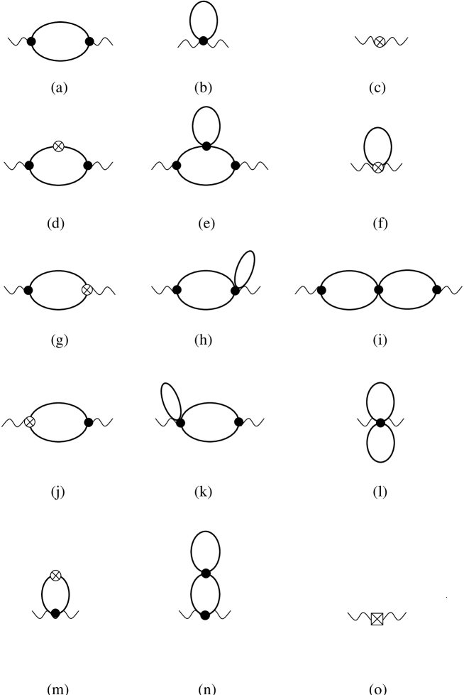
Figure 1: Diagrams for the vector two-point function. The crossed circle stands for the ${\cal O}(p^{4})$ vertex insertion. Wiggly lines are the external vector currents. Dots are ${\cal O}(p^{2})$ vertices and a square is a ${\cal O}(p^{6})$ vertex. The solid lines are meson propagators.

We have performed the following checks

1. In the isospin and hypercharge case the longitudinal part vanishes.

2. In the SU(3) limit, i.e. $m_{\pi}^{2}=m_{K}^{2}=m_{\eta}^{2}\to m_{chiral}^{2}$, all two-point functions are equal.

3. The SU(3) breaking effect in the form-factors appears only in second order in the quark masses, i.e. order $(m_{s}-\hat{m})^{2}$, as required by the Ademollo-Gatto theorem [19].

4. All divergences with a non-analytical dependence on masses or $q^{2}$ cancel and the $\ln(4\pi)$ and $\gamma$ terms can be absorbed in the counter-terms as well. Both of these follow from general renormalizability theorems.

5. The remaining divergences are in agreement with those from the general calculation using heat-kernel methods [20] and with the double logarithms of [21].

The result can be expressed simply in terms of the finite functions

$$\mu_{i} = \frac{m_{i}^{2}}{32\pi^{2}}\ln\frac{m_{i}^{2}}{\mu^{2}}\;,$$

$$B_{V}^{ij}(q^{2}) = \frac{1}{q^{2}}\left\{{B}_{22}(m_{i}^{2},m_{j}^{2},q^{2})-\frac{\lambda_{0}}{64\pi^{2}}\left(m_{i}^{2}+m_{j}^{2}-\frac{q^{2}}{3}\right)+\frac{1}{2}(\mu_{i}+\mu_{j})\right\}\,,$$

for $i,j=\pi,K,\eta$. The definitions of $B_{22}(m_{i}^{2},m_{j}^{2},q^{2})$ and $\lambda_{0}$ can be found in App. C.1. Notice that $B_{V}^{ii}(q^{2})$ is regular at $q^{2}=0$ for $i=j$.

For the isospin transverse part we find

$$\Pi_{V\pi}^{(1)}(q^{2})=-4(2H_{1}^{r}+L_{10}^{r})-8{B}_{V}^{\pi\pi}(q^{2})-4{B}_{V}^{KK}(q^{2})$$

$$+\frac{1}{F^{2}_{\pi}}\bigg{\{}-16\bigg{(}2q^{2}{B}_{V}^{\pi\pi}(q^{2})+q^{2}{B}_{V}^{KK}(q^{2})\bigg{)}L_{9}^{r}+16q^{2}(2\mu_{\pi}+\mu_{K})(L_{9}^{r}+L_{10}^{r})$$

$$+4q^{2}\bigg{(}2{B}_{V}^{\pi\pi}(q^{2})+{B}_{V}^{KK}(q^{2})\bigg{)}^{2}\bigg{\}}-32m_{\pi}^{2}C^{r}_{61}-32(m_{\pi}^{2}+2m_{K}^{2})C^{r}_{62}-8q^{2}C^{r}_{93}\,.$$

The hypercharge transverse part is given by

$$\Pi_{V\eta}^{(1)}(q^{2})=-4(2H_{1}^{r}+L_{10}^{r})-12{B}_{V}^{KK}(q^{2})$$ (20)

$$+\frac{1}{F^{2}_{\pi}}\bigg{\{}-48q^{2}{B}_{V}^{KK}(q^{2})L_{9}^{r}+48\mu_{K}(L_{9}^{r}+L_{10}^{r})+36q^{2}({B}_{V}^{KK}(q^{2}))^{2}\bigg{\}}$$

$$-32m_{\eta}^{2}C^{r}_{61}-32(m_{\pi}^{2}+2m_{K}^{2})C^{r}_{62}-8q^{2}C^{r}_{93}\;.$$

The longitudinal part vanishes for the above two. These results agree with those obtained in [5] when the differences in subtraction schemes are taken into account.

The expressions for the kaon two-point functions are new and are somewhat longer. The transverse part is given by

$$\Pi_{VK}^{(1)}(q^{2})=-4(2H_{1}^{r}+L_{10}^{r})-6({B}_{V}^{\pi K}(q^{2})+{B}_{V}^{\eta K}(q^{2}))$$ (21)

$$+\frac{1}{F^{2}_{\pi}}\bigg{\{}-\frac{8}{q^{2}}(m_{K}^{2}-m_{\pi}^{2})(3\mu_{\pi}-2\mu_{K}-\mu_{\eta})L_{5}^{r}+12(\mu_{\pi}+2\mu_{K}+\mu_{\eta})(L_{9}^{r}+L_{10}^{r})$$

$$-24q^{2}\bigg{(}{B}_{V}^{\pi K}(q^{2})+{B}_{V}^{\eta K}(q^{2})\bigg{)}L_{9}^{r}-\frac{3}{4q^{2}}(5\mu_{\pi}\mu_{\pi}-4\mu_{K}\mu_{K}-3\mu_{\eta}\mu_{\eta}-4\mu_{\pi}\mu_{K}$$

$$-6\mu_{\pi}\mu_{\eta}+12\mu_{K}\mu_{\eta})+9q^{2}\bigg{(}{B}_{V}^{\pi K}(q^{2})+{B}_{V}^{\eta K}(q^{2})\bigg{)}^{2}\bigg{\}}-\frac{32}{q^{2}}(m_{\pi}^{2}-m_{K}^{2})^{2}C^{r}_{38}$$

$$-32m_{K}^{2}C^{r}_{61}-32(m_{\pi}^{2}+2m_{K}^{2})C^{r}_{62}-\frac{8}{q^{2}}(m_{\pi}^{2}-m_{K}^{2})^{2}C^{r}_{91}-8q^{2}C^{r}_{93}\;.$$

This two-point function has also a longitudinal part

$$\Pi_{VK}^{(0)}(q^{2})=\frac{3}{2q^{4}}\bigg{(}(m_{K}^{2}-m_{\pi}^{2})^{2}\bar{J}^{\pi K}(q^{2})+(m_{K}^{2}-m_{\eta}^{2})^{2}\bar{J}^{\eta K}(q^{2})\bigg{)}$$ (22)

$$+\frac{1}{q^{2}F^{2}_{\pi}}\bigg{\{}\bigg{(}8(m_{K}^{2}-m_{\pi}^{2})(3\mu_{\pi}-2\mu_{K}-\mu_{\eta})+12(m_{K}^{2}-m_{\pi}^{2})^{2}\bar{J}^{\pi K}(q^{2})$$

$$+12(m_{K}^{2}-m_{\eta}^{2})^{2}\bar{J}^{\eta K}(q^{2})\bigg{)}L_{5}^{r}+\frac{3}{4}(5\mu_{\pi}\mu_{\pi}-4\mu_{\pi}\mu_{K}-6\mu_{\pi}\mu_{\eta}-4\mu_{K}\mu_{K}$$

$$+12\mu_{K}\mu_{\eta}-3\mu_{\eta}\mu_{\eta})-\frac{3}{4}(-5\mu_{\pi}+2\mu_{K}+3\mu_{\eta})(m_{K}^{2}-m_{\pi}^{2})\bar{J}^{\pi K}(q^{2})$$

$$-\frac{9}{4}(\mu_{\pi}-2\mu_{K}+\mu_{\eta})(m_{K}^{2}-m_{\eta}^{2})\bar{J}^{\eta K}(q^{2})+\frac{3}{2}\left((m_{K}^{2}-m_{\pi}^{2})\bar{J}^{\pi K}(q^{2})\right)^{2}$$

$$-\frac{9}{16}\bigg{(}(m_{K}^{2}-m_{\pi}^{2})\bar{J}^{\pi K}(q^{2})+(m_{K}^{2}-m_{\eta}^{2})\bar{J}^{\eta K}(q^{2})\bigg{)}^{2}$$

$$+\frac{1}{q^{2}}\bigg{(}-\frac{3}{8}(m_{\pi}^{2}+m_{K}^{2})\left((m_{K}^{2}-m_{\pi}^{2})\bar{J}^{\pi K}(q^{2})\right)^{2}$$

$$+\frac{3}{4}(m_{\pi}^{2}+m_{K}^{2})(m_{K}^{2}-m_{\pi}^{2})(m_{K}^{2}-m_{\eta}^{2})\bar{J}^{\pi K}(q^{2})\bar{J}^{\eta K}(q^{2})$$

$$-(\frac{3}{8}m_{\pi}^{2}-\frac{13}{8}m_{K}^{2})\left((m_{K}^{2}-m_{\eta}^{2})\bar{J}^{\eta K}(q^{2})\right)^{2}\bigg{)}$$

$$-\frac{9}{16q^{4}}\bigg{(}(m_{K}^{2}-m_{\pi}^{2})^{2}\bar{J}^{\pi K}(q^{2})+(m_{K}^{2}-m_{\eta}^{2})^{2}\bar{J}^{\eta K}(q^{2})\bigg{)}^{2}\bigg{\}}$$

$$+\frac{8}{q^{2}}(m_{\pi}^{2}-m_{K}^{2})^{2}(4C^{r}_{38}+C^{r}_{91})\;,$$

Notice that the Ademollo-Gatto theorem [19] is explicitly satisfied.

All divergences have been absorbed in the coefficients of the ${\cal O}(p^{6})$ Lagrangian by setting

$$\mu^{4\epsilon}(4C_{38}+C_{91}) = 4C^{r}_{38}+C^{r}_{91}+\frac{5}{32F_{0}^{2}}\lambda_{2}-\frac{5}{3F_{0}^{2}}\lambda_{1}L^{r}_{5}\;,$$

$$\mu^{4\epsilon}C_{61} = C^{r}_{61}-\frac{3}{8F_{0}^{2}}\lambda_{1}(L^{r}_{9}+L^{r}_{10})\;,$$

$$\mu^{4\epsilon}C_{62} = C^{r}_{62}-\frac{1}{8F_{0}^{2}}\lambda_{1}(L^{r}_{9}+L^{r}_{10})\;,$$

$$\mu^{4\epsilon}C_{93} = C^{r}_{93}-\frac{1}{32F_{0}^{2}}\lambda_{2}+\frac{1}{2F_{0}^{2}}\lambda_{1}L^{r}_{9}\;,$$ (23)

which agrees with the calculation of [20].

5 Masses and Decay Constants

5.1 Masses

The definition of mass is the position of the pole in a two-point Green function $G(p^{2},m^{2})$ that contains the relevant particle as a possible intermediate state. The axial-vector two-point function is a suitable candidate to obtain the masses for the pseudoscalar mesons. The general structure of this two-point function is shown in terms of one-particle-irreducible (1PI) diagrams in Fig. 2.

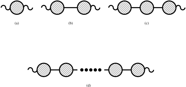
Figure 2: The diagrams contributing to the axial-vector two-point function. The filled circles indicate the one-particle-irreducible diagrams. Solid lines are pseudoscalar meson propagators and the wiggly lines indicate insertions of an axial-vector current. For the inverse propagator the wiggly lines are meson legs and for the decay constant the right wiggly line is a meson leg while the left remains an axial current.

However the meson-propagator or the two-point function of meson fields itself is a simpler set with the same pole. We denote the sum of 1PI graphs by $i\Pi(p^{2},m_{i0}^{2},F_{0})$. The set of diagrams contributing to $\Pi(p^{2},m_{i0}^{2},F_{0})$ is depicted in Fig. 3(c).

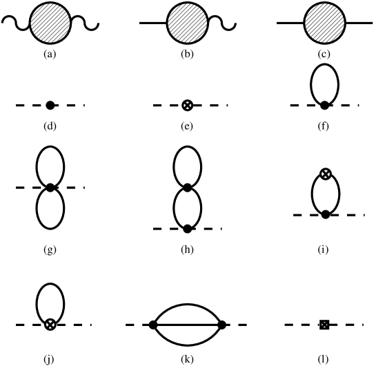
Figure 3: The set of diagrams contributing to the 1PI quantities. (a) axial-vector–axial-vector (b) axial-vector–pseudoscalar (c) pseudoscalar–pseudoscalar. (d)-(l) the respective diagrams when the dashed lines are replaced with the external legs of (a), (b) or (c). A line is a meson propagator, a wiggly line an external source, a dot a vertex of ${\cal O}(p^{2})$, a crossed circle a vertex of ${\cal O}(p^{4})$ and a crossed box a vertex of ${\cal O}(p^{6})$.

The propagator is

$$G(p^{2},m_{i0}^{2},F_{0}) = \frac{i}{p^{2}-m_{0}^{2}}\sum_{n=0}^{\infty}\left(i\Pi(p^{2},m_{i0}^{2},F_{0})\frac{i}{p^{2}-m_{0}^{2}}\right)^{n}$$ (24)

$$= \frac{i}{p^{2}-m_{0}^{2}+\Pi(p^{2},m_{i0}^{2},F_{0})}\,,$$

where $m_{0}^{2}$ stands for the lowest order mass and $m_{i0}^{2}$ collectively denotes the various lowest order masses. The physical mass is given by the zero of the denominator once the external legs are on mass-shell

$$m_{phys}^{2}-m_{0}^{2}+\Pi(m_{phys}^{2},m_{i0}^{2},F_{0})=0\,.$$ (25)

We replace the masses $m_{i0}$ by their physical masses and $F_{0}$ by $F_{\pi}$. It is sufficient to use the NLO formulae for these in $\Pi(p^{2},m_{i0}^{2},F_{0})$ since it is already of ${\cal O}(p^{4})$. This leads to

$$m_{phys}^{2}=m_{0}^{2}+(m^{2})^{(4)}+(m^{2})^{(6)}\,,$$ (26)

where the bare masses appear only at the leading order and superscripts refer to the chiral order.

The resulting formulae for the pion, kaon and eta masses are gathered in App. A.1. The formulae for the pion and eta mass agree with those of [6] (the explicit formulae only appear in the preprint version) in the way described earlier, see footnote 1, while the kaon result is new.

Notice that the precise expression for the ${\cal O}(p^{6})$ is dependent on the choice of the ${\cal O}(p^{4})$ expression, using the Gell-Mann-Okubo relation at ${\cal O}(p^{4})$, produces differences at ${\cal O}(p^{6})$.

The masses depend on seven combinations of the ${\cal O}(p^{6})$ constants. All the relevant checks described in Sect. 4 were done.

5.2 Decay Constants

The pseudoscalar decay constants, $F_{a}$, are defined by

$$\langle 0|A^{a}(0)_{\mu}|\phi^{a}(p)\rangle=i\sqrt{2}p_{\mu}F_{a}\,.$$ (27)

They can be obtained directly from the definition or by the residue of the pole in the axial-vector two-point function. We have calculated them first using their definition and verified that the calculation via the two-point function yields the same results.

This calculation involves the use of the expression for $\Pi(p^{2},m_{i0}^{2},F_{0})$ obtained earlier to get the wavefunction renormalization in addition to those diagrams of Fig. 3(b) for the matrix element itself.

We can then write the results in the form

$$F_{a}=F_{0}\left(1+\bar{F}_{a}^{(4)}+\bar{F}_{a}^{(6)}\right)\,.$$ (28)

Similarly to the masses, the precise form of $\bar{F}_{a}^{(6)}$ depends on the choice of $\bar{F}_{a}^{(4)}$. For $F_{\pi}$ and $F_{\eta}$ we have checked the double logarithms with those presented in [6] and the result for $F_{K}$ is new.

The explicit formulae are rather long and can be found in App. A.2. The relevant checks described in Sect. 4 were performed.

6 The Axial-Vector Two-Point Functions

The axial-vector two-point functions to lowest order are quite simple and all three reduce to

$$\Pi^{Aa}_{\mu\nu}(q)=2F_{0}^{2}g_{\mu\nu}-\frac{2F_{0}^{2}}{q^{2}-m^{2}_{0a}}q_{\mu}q_{\nu}\,.$$ (29)

The NLO corrections only introduce minor changes. The decay constants change to $F_{a}$, the masses to the physical ones and there is an additional contribution from the ${\cal O}(p^{4})$ constants to $\Pi^{(1)}_{Aa}(q^{2})=4L_{10}^{r}-8H_{1}^{r}$. In fact a very large part of the ${\cal O}(p^{6})$ corrections is of a similar nature. We thus define

$$\Pi^{Aa}_{\mu\nu}(q)=2F^{2}_{a}g_{\mu\nu}-\frac{2F^{2}_{a}}{q^{2}-m^{2}_{a}}q_{\mu}q_{\nu}+(q_{\mu}q_{\nu}-g_{\mu\nu}q^{2})\hat{\Pi}^{(1)}_{Aa}(q^{2})+q_{\mu}q_{\nu}\hat{\Pi}^{(0)}_{Aa}(q^{2})\,.$$ (30)

The function $\hat{\Pi}^{(1)}_{Aa}(q^{2})$ can be fully calculated from diagram (a) of Fig. 2. These are depicted in more detail in Fig. 3(d-l) and discussed in App. B.1.

All the diagrams in Fig. 2 contribute to $\hat{\Pi}^{(0)}_{Aa}(q^{2})$ even though most of their contents actually go into the redefinitions of the respective decay constants and masses. The full result is given in App. B.2. The results fulfill the same checks as in Sect. 4. We call $\hat{\Pi}^{(0)}_{Aa}(q^{2})$ and $\hat{\Pi}^{(1)}_{Aa}(q^{2})$ the longitudinal and transverse remainder respectively.

7 Estimates of some ${\cal O}(p^{6})$ constants

In this section we estimate some of the ${\cal O}(p^{6})$ constants that appear in the results. We assume saturation by the lightest vector, axial-vector and scalar mesons, extending the formalism used in [7] to the present case.

For the spin-1 mesons we use the realization where the vector contribution to the chiral Lagrangian starts at ${\cal O}(p^{6})$. Keeping only the relevant terms for our calculation we have

$${\cal L}_{V}=-\frac{1}{4}\langle V_{\mu\nu}V^{\mu\nu}-2M^{2}_{V}V_{\mu}V^{\mu}\rangle-\frac{f_{V}}{2\sqrt{2}}\langle V_{\mu\nu}f^{\mu\nu}_{+}\rangle+\ldots\,,$$ (31)

where

$$V_{\mu\nu}=\nabla_{\mu}V_{\nu}-\nabla_{\nu}V_{\mu}\,, f^{\mu\nu}_{\pm}=u(v_{\mu\nu}-a_{\mu\nu})u^{\dagger}\pm u^{\dagger}(v_{\mu\nu}+a_{\mu\nu})u\,,$$

and the same holds for the axial-vector with the label change $V\leftrightarrow A$ and $f_{+}\leftrightarrow f_{-}$. $V_{\mu}$ and $A_{\mu}$ are three-by-three matrices in flavour space and describe the full vector and axial-vector nonets, thus we assume a nonet symmetry throughout the rest of this section. The rest of the notations was already presented in Sect. 3.

After integrating out the vectors the terms contributing to the two-point Green functions at ${\cal O}(p^{6})$ are

$${\cal L}_{V,A}=\frac{f_{V}^{2}}{4M^{2}_{V}}\langle f^{\mu\nu}_{+}\nabla_{\mu}\nabla_{\lambda}f^{\lambda\nu}_{+}\rangle+\frac{f_{A}^{2}}{4M^{2}_{A}}\langle f^{\mu\nu}_{-}\nabla_{\mu}\nabla_{\lambda}f^{\lambda\nu}_{-}\rangle\,.$$ (32)

In the scalar case, the Lagrangian reads

$${\cal L}_{S} = \frac{1}{2}\langle\nabla^{\mu}S\nabla_{\mu}S-M^{2}_{S}S^{2}\rangle+c_{d}\langle Su^{\mu}u_{\mu}\rangle+c_{m}\langle S\chi_{+}\rangle+\frac{d_{m}}{2}\langle S^{2}\chi_{+}\rangle$$ (33)

$$+c_{\gamma}\langle Sf_{+\mu\nu}f_{+}^{\mu\nu}\rangle+c^{\prime}_{\gamma}\langle Sf_{-\mu\nu}f_{-}^{\mu\nu}\rangle\,.$$

After integrating out the scalars, the ${\cal O}(p^{6})$ contribution we are interested in comes from the terms

$${\cal L}_{S}=\frac{-c^{2}_{m}}{2M^{4}_{S}}\langle\chi_{+}\nabla^{2}\chi_{+}\rangle+\frac{d_{m}c_{m}^{2}}{2M^{4}_{S}}\langle\chi_{+}^{3}\rangle+\frac{c_{d}c_{m}d_{m}}{M^{4}_{S}}\langle\chi_{+}^{2}u_{\mu}u^{\mu}\rangle+\frac{c_{m}c_{\gamma}}{M^{2}_{S}}\langle\chi_{+}f_{+\mu\nu}f_{+}^{\mu\nu}\rangle\,,$$ (34)

obtained after the shift of the vacuum expectation value and using the equation of motion for the scalars. Note that only the relevant terms are written and, as in the vector and axial case, a full nonet of scalars is assumed in $S$.

As input parameters we use

$$M_{V}=M_{\rho}=0.77\mbox{ GeV}, f_{V}=0.20,\quad M_{A}=M_{a_{1}}=1.23\mbox{ GeV},\quad f_{A}=0.10,$$

$$M_{S}=0.93\mbox{ GeV}, c_{m}=0.042\mbox{ GeV},\quad c_{d}=0.032\mbox{ GeV},$$

$$c_{\gamma}=19\cdot 10^{-3}\mbox{ GeV}^{-1}, c^{\prime}_{\gamma}\sim c_{\gamma}\quad\mbox{and}\quad d_{m}=-2.4\,.$$ (35)

$M_{S}$ and $d_{m}$ are obtained from the masses of the scalars $K^{*}_{0}(1430)$ and $a_{0}(980)$. The value $c_{\gamma}$ is obtained from $\Gamma(f_{0}\rightarrow\gamma\gamma)=0.56\pm 0.11$ keV and is compatible also with $\Gamma(a_{0}\to\gamma\gamma)=0.30\pm 0.10$ keV. The values of $c_{m}$ and $c_{d}$ are obtained forcing the saturation of some of the ${\cal O}(p^{4})$ constants by the scalars [7] and are compatible with those obtained in $\Gamma(a_{0}\to\pi\eta)$. $c^{\prime}_{\gamma}$ value cannot be determined from data at present, we assume a value similar to $c_{\gamma}$.

Using the notation of [8] for the ${\cal O}(p^{6})$ terms, the spin-1 Lagrangian yields

$$C^{r}_{87}\sim\frac{1}{8}\left(\frac{f^{2}_{V}}{M^{2}_{V}}-\frac{f^{2}_{A}}{M^{2}_{A}}\right)\sim 7.6\cdot 10^{-3}\,\mbox{ GeV}^{-2}\,,$$ (36)

$$C^{r}_{93}\sim-\frac{f^{2}_{V}}{4M^{2}_{V}}\sim-17\cdot 10^{-3}\,\mbox{ GeV}^{-2}\,,$$ (37)

and the scalar Lagrangian estimates

$$C^{r}_{14}\sim\frac{c_{d}c_{m}d_{m}}{M^{4}_{S}}\sim-4.3\cdot 10^{-3}\,\mbox{ GeV}^{-2}\,,$$ (38)

$$C^{r}_{19}\sim\frac{d_{m}c^{2}_{m}}{2M^{4}_{S}}\sim-2.8\cdot 10^{-3}\,\mbox{ GeV}^{-2}\,,$$ (39)

$$C^{r}_{38}\sim\frac{c^{2}_{m}}{2M^{4}_{S}}\sim 1.2\cdot 10^{-3}\,\mbox{ GeV}^{-2}\,,$$ (40)

$$C^{r}_{61}\sim\frac{c_{m}c_{\gamma}}{M^{2}_{S}}\sim 1.9\cdot 10^{-3}\,\mbox{ GeV}^{-2}\,,$$ (41)

$$C^{r}_{80}\sim\frac{c_{m}c^{\prime}_{\gamma}}{M^{2}_{S}}\sim 1.9\cdot 10^{-3}\,\mbox{ GeV}^{-2}\,.$$ (42)

We stress that the goal of this section is to roughly estimate the values of the ${\cal O}(p^{6})$ constants. A real determination would imply the use of chiral sum rules or other processes to fix them. It is worth mentioning that the result in Eq. (37) is the same if we use an antisymmetric formalism for the vector Lagrangian, and is in agreement with the result extracted from the experimental data using sum rules for the vector-vector two-point functions [9]. The generalization to the three flavours introduces a new relation of ${\cal O}(p^{6})$ constants, $4C^{r}_{38}+C^{r}_{91}$, due to the explicit chiral symmetry breaking in the kaon Green function.

Finally, we remark that the precise value of the constants can have an important variation depending of the input values in Eq. (7). Consequently, although the values cited in this section are used for the numerical results, with the understanding that the other counter-terms are set to zero, we have to keep in mind that these values could overestimate the physical ones. The latter is especially true for $d_{m}$ since the $K_{0}$ and $a_{0}$ mass difference appears unnaturally large.

8 Some numerical results

We defer a more accurate comparison with experimental data to [11], but we would like to present some results using our explicit expressions. We use the values for the $C_{i}^{r}$ obtained in the previous section and two sets of the ${\cal O}(p^{4})$ constants. They only differ in the values of $L_{1}^{r}$, $L_{2}^{r}$ and $L_{3}^{r}$. Set A is obtained from the fit of the unitarized $K_{l4}$ calculation while set B refers to $K_{l4}$ and $\pi\pi$ data at one loop accuracy [22]. We give both sets to show an example of the variation with the ${\cal O}(p^{4})$ constants. We do not show results for varying the other $L_{i}^{r}$ but this results in a similar variation in size of the ${\cal O}(p^{6})$ results. The explicit values we use, at $\mu=0.77~{}GeV$, are

$$L_{1}^{r} = 0.37\cdot 10^{-3},\quad L_{2}^{r}=1.35\cdot 10^{-3},\quad L_{3}^{r}=-3.5\cdot 10^{-3}\quad\mbox{{\bf set A}}$$

$$L_{1}^{r} = 0.60\cdot 10^{-3},\quad L_{2}^{r}=1.50\cdot 10^{-3},\quad L_{3}^{r}=-3.3\cdot 10^{-3}\quad\mbox{{\bf set B}}$$

$$L_{4}^{r} = -0.3\cdot 10^{-3},\quad L_{5}^{r}=1.4\cdot 10^{-3},\quad L_{6}^{r}=-0.2\cdot 10^{-3},$$

$$L_{7}^{r} = -0.4\cdot 10^{-3},\quad L_{8}^{r}=0.9\cdot 10^{-3},\quad L_{9}^{r}=6.9\cdot 10^{-3},$$

$$L_{10}^{r} = 1/4(f_{V}^{2}-f_{A}^{2})=-7.5\cdot 10^{-3},$$

$$H_{1}^{r} = 1/8(f_{V}^{2}+f_{A}^{2})=6.25\cdot 10^{-3}.$$

For $H_{1}^{r}$, which can not be obtained experimentally, we take the value from the Meson Saturation Model. Because the vector contribution should cancel for the axial-vector two-point function, we use the same model value for $L^{r}_{10}$.

The rest of the quantities we use are

$$m_{\pi}=0.135\,{\rm GeV},\quad m_{K}=0.495\,{\rm GeV},\quad m_{\eta}=0.548\,{\rm GeV}~{}~{}\mbox{and}~{}~{}F_{\pi}=0.0924\,{\rm GeV}.$$ (44)

They seem reasonable averages of the various isospin related ones.

8.1 The Vector Two-Point Functions

In Fig. 4 and Fig. 5 we plot the real part of the three vector-vector two-point functions choosing set A inputs.

Figure 4: Different contributions to the real part of the vector-vector two-point function in the isospin and the hypercharge case. The label CT indicates the contribution from only the counter-terms $L_{i}^{r}$ at ${\cal O}(p^{4})$ and $C_{i}^{r}$ at ${\cal O}(p^{6})$. $p^{4}$ gives the ${\cal O}(p^{4})$ result. VMD indicates the vector model of Eq. (45).

In all the three cases the slopes are given mainly by the ${\cal O}(p^{6})$ constants as estimated above. We have shown these contributions in the curves labeled (CT). Essentially — and with exception of $C^{r}_{93}$ — the main effect of varying the input parameters is to shift the plots vertically. We see that the loop effects are larger in the isospin case and smaller for both, the hypercharge and kaon. In the chiral limit all three cases reduce to the same, and differences are related to the breaking of the $SU(3)$ symmetry. For the isospin, the two-pion channel produces the notable difference with the counter-term contribution, while for the hypercharge and kaon the smaller difference is explained by the larger masses in the loops and some explicit breaking of the symmetry through the quark masses in the counter-term contributions.

Figure 5: Different contributions to the real part of the kaon vector-vector two-point function. The superscripts L (T) refers to the longitudinal (transverse) part. For comparison we also plot the isospin case. (CT) as in Fig. 4.

In Fig. 4 we also plotted the case with a complete saturation by the vector meson (VMD)

$$Re(\,\Pi_{V}\,)\sim\frac{2f_{V}^{2}(1-\frac{q2}{M^{2}_{V}})}{(1-\frac{q^{2}}{M^{2}_{V}})^{2}+\frac{\Gamma^{2}}{M^{2}_{V}}},\,$$ (45)

with $\Gamma=0.150\,{\rm GeV}$. The conclusion is that models with only vectors explain the main part of the two-point function, however an important contribution coming from the two-pion intermediate states is present. The curve including only the counter terms —isospin (CT)— can also be obtained with the first two terms of the expansion in the previous formula with $\Gamma=0$ and considering the tiny modification due to the scalars.

8.2 Masses and Decay Constants

We continue our discussion with the masses and decay constants. We have summarized our numerical results in Table 1 using the values for the ${\cal O}(p^{4})$ constants quoted above. As one sees in columns three to six, both masses and decay constants have substantial ${\cal O}(p^{6})$  loop contributions. In addition the pure polynomial piece at ${\cal O}(p^{6})$ tends to have the opposite sign and is very large using our model dependent estimates. This only reinforces the statement in Sect. 7 of the lack of knowledge in the scalar sector. The terms containing $d_{m}$ are the only ones contributing in this subsection and seem severely overestimated even though they are of a size expected by naive dimensional analysis.

	${\cal O}(p^{4})$	set A	set A	set A	set B	$C_{i}^{r}$
$\mu$ (GeV)	0.77	0.77	0.5	1.0	0.77	$-$
$F_{\pi}/F_{0}$	0.068	$-$0.101	$-$0.066	$-$0.100	$-$0.172	$-$0.001
$(F_{\pi}/F_{0})$		(0.013)			($-$0.050)
$F_{K}/F_{\pi}$	0.216	0.055	$-$0.023	0.100	0.035	$-0.450$
($F_{K}/F_{\pi}$)		(0.08)			(0.06)
$F_{\eta}/F_{\pi}$	0.312	0.092	$-$0.011	0.150	0.065	$-0.600$
$m_{\pi}^{2}/m_{\pi phy}^{2}$	$-$0.039	0.214	0.132	0.238	0.355	$-$0.003
$m_{K}^{2}/m_{Kphy}^{2}$	$-$0.003	0.241	0.246	0.194	0.423	$-$0.873
$m_{\eta}^{2}/m_{\eta phy}^{2}$	$-$0.045	0.312	0.234	0.273	0.521	$-$2.428

Table 1: ${\cal O}(p^{4})$ and ${\cal O}(p^{6})$ contributions to the masses and decay constants. The number in brackets are the extended double log approximation of Ref. [21]. Columns three to six are the ${\cal O}(p^{6})$ loop contributions only. The contribution from the $C_{i}^{r}$ is listed separately in the last column.

In order to have a full presentation of the ${\cal O}(p^{6})$ contributions a refit of all ${\cal O}(p^{4})$ coefficients using the full ${\cal O}(p^{6})$ expressions would be needed. We postpone this till after the main other processes are also calculated to this order given the dependence of the ${\cal O}(p^{6})$ contributions on $L^{r}_{1}$–$L^{r}_{3}$. As an example using set A at $\mu=0.77~{}GeV$ otherwise but shifting $L_{5}^{r}$ to $1.0\cdot 10^{-3}$ reproduces the experimental value of $F_{K}/F_{\pi}$ when setting $d_{m}=0$.

For the decay constants the ${\cal O}(p^{6})$ contributions to the ratios are smaller than the ${\cal O}(p^{4})$, not including the estimates from scalar exchange to the ${\cal O}(p^{6})$ constants.

To judge the effect of the ${\cal O}(p^{6})$ contributions on determining the quark mass ratios we use the lowest order, ${\cal O}(p^{4})$ and ${\cal O}(p^{6})$ formulae in terms of physical quantities to obtain the lowest order masses using Eq. (26). This leads to

$$\frac{2m_{s}}{m_{u}+m_{d}} = \frac{2m_{0K}^{2}-m_{0\pi}^{2}}{m_{0\pi}^{2}}=25.9(p^{2});\quad 24.9(p^{4});\quad 24.1(p^{6})\quad\mbox{and}$$

$$\frac{2m_{s}}{m_{u}+m_{d}} = \frac{3m_{0\eta}^{2}-m_{0\pi}^{2}}{2m_{0\pi}^{2}}=24.2(p^{2});\quad 24.4(p^{4});\quad 23.3(p^{6})$$ (46)

using the results from set A at $\mu=0.77~{}GeV$ and $C^{r}_{i}=0$. These ratios can be compared with $2m_{s}/(m_{u}+m_{d})=25.5~{}\cite[cite]{[\@@bibref{}{ximojamin}{}{}]};\,22.8~{}\cite[cite]{[\@@bibref{}{lattice}{}{}]}$ , extracted from QCD sum rules and lattice calculations respectively.

The emerging conclusions about the convergence of the chiral series should be very cautious since a full study includes also the effect of the ${\cal O}(p^{6})$ constants. However, while the corrections calculated are significant they do not show evidence of a breakdown of the chiral expansion for the quantities presented here.

8.3 The Axial-Vector Two-Point Functions

In Fig. 6 we plotted the dependence on momenta of the real part for the remainders of the axial-vector two-point functions for the three cases under study. Because both the longitudinal and transverse remainders have poles at $q^{2}=0$, we show the combination ${\hat{\Pi}}_{A}^{(1)}+{\hat{\Pi}}_{A}^{(0)}$. A priori we would expect a different behaviour for the isospin case due to the three pion channel. However there is virtually no effect because the imaginary part is very small in the energy region we are considering in agreement with the dominance of the $a_{1}$ axial meson. For the other two cases even the three pseudoscalar channel is far. The curves are thus very linear. The vertical shifts are due to the explicit breaking from the quark masses. The ${\cal O}(p^{6})$ contributions are rather small, the scale in the plot should be compared with $|2F_{\pi}^{2}/q^{2}|$ which is larger than 0.07 for the entire region plotted.

Figure 6: Different contributions to the real part of the remainder axial-axial two-point function. The superscripts L (T) refers to the remainder longitudinal (transverse) part. (CT) as in Fig 4.

9 Summary and Conclusions

In this paper we have calculated to NNLO in CHPT the vector and axial-vector two-point functions in the isospin limit and in the complete three flavour basis.

In the vector-vector case, we confirm previous results for the isospin and hypercharge [5].

For the axial-vector case, besides the cancellation of the non-analytic poles, we obtain the same double and simple poles that appear with the use of the heat kernel expansion [20]. We also agree with the double logarithms, appearing in previous work [6], for the isospin and hypercharge cases. All these checks give us confidence about our result.

We have also given expressions to NNLO for the masses and decay constants. The Lagrangian at ${\cal O}(p^{6})$ contains a rather large number of free constants. We have estimated some of them using a simple resonance estimate and used this to present some first numerical results for the two-point functions, masses and decay constants. We also studied somewhat the $\mu$-dependence of the final result.

Although the corrections are significant they do not show evidence of a breakdown of the chiral expansion. For instance, our estimates of the quark mass ratios are in agreement with previous determinations. However, the sensitivity to the input values, indicate that the ${\cal O}(p^{4})$ constants need to be refitted using the full ${\cal O}(p^{6})$ expressions and that better estimates of the ${\cal O}(p^{6})$ constants are necessary.

Appendix A Explicit results for the masses and decay constants

A.1 Masses

The masses are split as follows

$$m_{a}^{2}=m_{0a}^{2}+(m_{a}^{2})^{(4)}+(m_{a}^{2})^{(6)}_{CT}+(m_{a}^{2})^{(6)}_{loops}\,.$$ (47)

with $m_{0a}$ the contribution from the bare masses. In the ${\cal O}(p^{6})$  we have explicitly separated the chiral loop contribution from the model dependent counter-terms.

In a previous step the masses are obtained in terms of only the bare masses (quark masses), we rewrite the ${\cal O}(p^{4})$ contribution with the physical masses implying a modification of the ${\cal O}(p^{6})$ terms. In the ${\cal O}(p^{6})$ we can safely replace bare masses with physical masses.

For the pion we obtain

$$m_{0\pi}^{2} = B_{0}(m_{u}+m_{d})=2B_{0}\hat{m}\,,$$

$$\frac{F_{\pi}^{2}}{m_{\pi}^{2}}(m_{\pi}^{2})^{(4)} = 8(m_{\pi}^{2}+2m_{K}^{2})(2L_{6}^{r}-L_{4}^{r})+8m_{\pi}^{2}(2L^{r}_{8}-L^{r}_{5})+\mu_{\pi}-\frac{1}{3}\mu_{\eta}$$ (48)

in agreement with [16]. The ${\cal O}(p^{6})$ contributions are

$$F_{\pi}^{2}(m_{\pi}^{2})^{(6)}_{CT}=-32m_{\pi}^{6}C^{r}_{12}-32m_{\pi}^{6}C^{r}_{13}-16m_{\pi}^{6}C^{r}_{14}-16m_{\pi}^{6}C^{r}_{15}-48m_{\pi}^{6}C^{r}_{16}$$ (49)

$$-16m_{\pi}^{6}C^{r}_{17}+48m_{\pi}^{6}C^{r}_{19}+80m_{\pi}^{6}C^{r}_{20}+48m_{\pi}^{6}C^{r}_{21}+32m_{\pi}^{6}C^{r}_{31}+32m_{\pi}^{6}C^{r}_{32}$$

$$-64m_{\pi}^{4}m_{K}^{2}C^{r}_{13}-32m_{\pi}^{4}m_{K}^{2}C^{r}_{15}+64m_{\pi}^{4}m_{K}^{2}C^{r}_{16}+192m_{\pi}^{4}m_{K}^{2}C^{r}_{21}$$

$$+64m_{\pi}^{4}m_{K}^{2}C^{r}_{32}-64m_{\pi}^{2}m_{K}^{4}C^{r}_{16}+64m_{\pi}^{2}m_{K}^{4}C^{r}_{20}+192m_{\pi}^{2}m_{K}^{4}C^{r}_{21}\,,$$

$$F_{\pi}^{4}(m_{\pi}^{2})^{(6)}_{Loops}=\frac{1}{(16\pi^{2})^{2}}\,(-527/1296\,m_{\pi}^{6}\,\pi^{2}-3217/1728\,m_{\pi}^{6}-37/324\,m_{\pi}^{4}\,m_{K}^{2}\,\pi^{2}$$ (50)

$$-139/216\,m_{\pi}^{4}\,m_{K}^{2}-11/36\,m_{\pi}^{2}\,m_{K}^{4}\,\pi^{2}-15/16\,m_{\pi}^{2}\,m_{K}^{4})$$

$$+\frac{1}{16\pi^{2}}\Bigg{(}\,(-2\,m_{\pi}^{4}-2\,m_{\pi}^{2}\,m_{K}^{2})\,\mu_{\pi}-2\,m_{\pi}^{2}\,m_{K}^{2}\,\mu_{K}+4\,m_{\pi}^{6}\,L_{1}^{r}\$$

$$+(74/9\,m_{\pi}^{6}-16/9\,m_{\pi}^{4}\,m_{K}^{2}+104/9\,m_{\pi}^{2}\,m_{K}^{4})\,L_{2}^{r}$$

$$+(56/27\,m_{\pi}^{6}-16/27\,m_{\pi}^{4}\,m_{K}^{2}+86/27\,m_{\pi}^{2}\,m_{K}^{4})\,L_{3}^{r}\,\Bigg{)}-(589/36\,m_{\pi}^{2}+2\,m_{K}^{2})\,\mu_{\pi}^{2}$$

$$-4\,m_{\pi}^{2}\,\mu_{\pi}\,\mu_{K}+5/3\,m_{\pi}^{2}\,\mu_{\pi}\,\mu_{\eta}-112\,m_{\pi}^{4}\,\mu_{\pi}\,L_{1}^{r}-64\,m_{\pi}^{4}\,\mu_{\pi}\,L_{2}^{r}$$

$$-56\,m_{\pi}^{4}\,\mu_{\pi}\,L_{3}^{r}+(144\,m_{\pi}^{4}+80\,m_{\pi}^{2}\,m_{K}^{2})\,\mu_{\pi}\,L_{4}^{r}+96\,m_{\pi}^{4}\,\mu_{\pi}\,L_{5}^{r}$$

$$+(-256\,m_{\pi}^{4}-160\,m_{\pi}^{2}\,m_{K}^{2})\mu_{\pi}\,L_{6}^{r}-176\,m_{\pi}^{4}\mu_{\pi}\,L_{8}^{r}+(-2/3\,m_{\pi}^{4}\,m_{K}^{-2}-7\,m_{\pi}^{2})\,\mu_{K}^{2}$$

$$-4/3\,m_{\pi}^{2}\mu_{K}\,\mu_{\eta}-128\,m_{\pi}^{2}\,m_{K}^{2}\,\mu_{K}\,L_{1}^{r}-32\,m_{\pi}^{2}\,m_{K}^{2}\,\mu_{K}\,L_{2}^{r}$$

$$-40\,m_{\pi}^{2}\,m_{K}^{2}\,\mu_{K}\,L_{3}^{r}+(16\,m_{\pi}^{4}+160\,m_{\pi}^{2}\,m_{K}^{2})\,\mu_{K}\,L_{4}^{r}+(16\,m_{\pi}^{4}+32\,m_{\pi}^{2}\,m_{K}^{2})\,\mu_{K}\,L_{5}^{r}$$

$$+(-32\,m_{\pi}^{4}-192\,m_{\pi}^{2}\,m_{K}^{2})\,\mu_{K}\,L_{6}^{r}+(-32\,m_{\pi}^{4}-64\,m_{\pi}^{2}\,m_{K}^{2})\,\mu_{K}\,L_{8}^{r}$$

$$+(-5/9\,m_{\pi}^{4}\,m_{\eta}^{-2}-29/36\,m_{\pi}^{2})\,\mu_{\eta}^{2}+(32/3\,m_{\pi}^{4}-128/3\,m_{\pi}^{2}\,m_{K}^{2})\,\mu_{\eta}\,L_{1}^{r}$$

$$+(8/3\,m_{\pi}^{4}-32/3\,m_{\pi}^{2}\,m_{K}^{2})\,\mu_{\eta}\,L_{2}^{r}+(8/3\,m_{\pi}^{4}-32/3\,m_{\pi}^{2}\,m_{K}^{2})\,\mu_{\eta}\,L_{3}^{r}$$

$$+(-16\,m_{\pi}^{4}+48\,m_{\pi}^{2}\,m_{K}^{2})\,\mu_{\eta}\,L_{4}^{r}+(-64/9\,m_{\pi}^{4}+64/9\,m_{\pi}^{2}\,m_{K}^{2})\,\mu_{\eta}\,L_{5}^{r}$$

$$+(64/3\,m_{\pi}^{4}-160/3\,m_{\pi}^{2}\,m_{K}^{2})\,\mu_{\eta}\,L_{6}^{r}+(-128/3\,m_{\pi}^{4}+128/3\,m_{\pi}^{2}\,m_{K}^{2})\,\mu_{\eta}\,L_{7}^{r}$$

$$-16/3\,m_{\pi}^{4}\,\mu_{\eta}\,L_{8}^{r}+(-128\,m_{\pi}^{6}-512\,m_{\pi}^{4}\,m_{K}^{2}-512\,m_{\pi}^{2}\,m_{K}^{4})\,L_{4}^{r2}$$

$$+(-256\,m_{\pi}^{6}-384\,m_{\pi}^{4}\,m_{K}^{2}-128\,m_{\pi}^{2}\,m_{K}^{4})\,L_{4}^{r}\,L_{5}^{r}\,$$

$$+(512\,m_{\pi}^{6}+2048\,m_{\pi}^{4}\,m_{K}^{2}+2048\,m_{\pi}^{2}\,m_{K}^{4})\,L_{4}^{r}\,L_{6}^{r}$$

$$+(512\,m_{\pi}^{6}+768\,m_{\pi}^{4}\,m_{K}^{2}+256\,m_{\pi}^{2}\,m_{K}^{4})\,L_{4}^{r}\,L_{8}^{r}$$

$$-128\,m_{\pi}^{6}\,L_{5}^{r2}+(512\,m_{\pi}^{6}+768\,m_{\pi}^{4}\,m_{K}^{2}+256\,m_{\pi}^{2}\,m_{K}^{4})\,L_{5}^{r}\,L_{6}^{r}$$

$$+512\,m_{\pi}^{6}\,L_{5}^{r}\,L_{8}^{r}+(-512\,m_{\pi}^{6}-2048\,m_{\pi}^{4}\,m_{K}^{2}-2048\,m_{\pi}^{2}\,m_{K}^{4})\,L_{6}^{r2}$$

$$+\,(-1024\,m_{\pi}^{6}-1536\,m_{\pi}^{4}\,m_{K}^{2}-512\,m_{\pi}^{2}\,m_{K}^{4})\,L_{6}^{r}\,L_{8}^{r}-512\,m_{\pi}^{6}\,L_{8}^{r2}$$

$$+5/6\,H^{F}(m_{\pi}^{2},m_{\pi}^{2},m_{\pi}^{2};m_{\pi}^{2})\,m_{\pi}^{4}-5/8\,H^{F}(m_{\pi}^{2},m_{K}^{2},m_{K}^{2};m_{\pi}^{2})\,m_{\pi}^{4}$$

$$+1/18\,H^{F}(m_{\pi}^{2},m_{\eta}^{2},m_{\eta}^{2};m_{\pi}^{2})\,m_{\pi}^{4}+H^{F}(m_{K}^{2},m_{\pi}^{2},m_{K}^{2};m_{\pi}^{2})\,m_{\pi}^{2}\,m_{K}^{2}$$

$$-5/6\,H^{F}(m_{K}^{2},m_{K}^{2},m_{\eta}^{2};m_{\pi}^{2})\,m_{\pi}^{4}-1/8\,H^{F}(m_{\eta}^{2},m_{K}^{2},m_{K}^{2};m_{\pi}^{2})\,m_{\pi}^{4}$$

$$+1/2\,H^{F}(m_{\eta}^{2},m_{K}^{2},m_{K}^{2};m_{\pi}^{2})\,m_{\pi}^{2}\,m_{K}^{2}+H^{F}_{1}(m_{\pi}^{2},m_{K}^{2},m_{K}^{2};m_{\pi}^{2})\,m_{\pi}^{4}$$

$$+2\,H^{F}_{1}(m_{K}^{2},m_{K}^{2},m_{\eta}^{2};m_{\pi}^{2})\,m_{\pi}^{4}+3\,H^{F}_{21}(m_{\pi}^{2},m_{\pi}^{2},m_{\pi}^{2};m_{\pi}^{2})\,m_{\pi}^{4}$$

$$-3/8\,H^{F}_{21}(m_{\pi}^{2},m_{K}^{2},m_{K}^{2};m_{\pi}^{2})\,m_{\pi}^{4}+3\,H^{F}_{21}(m_{K}^{2},m_{\pi}^{2},m_{K}^{2};m_{\pi}^{2})\,m_{\pi}^{4}$$

$$+9/8\,H^{F}_{21}(m_{\eta}^{2},m_{K}^{2},m_{K}^{2};m_{\pi}^{2})\,m_{\pi}^{4}\,.$$

Where the definitions of $H^{F}_{i}(m^{2}_{1},m^{2}_{2},m^{2}_{3};q^{2})$ appear in App. C.

For the kaon we obtain

$$m_{0K}^{2} = B_{0}(m_{s}+\hat{m})\,,$$

$$\frac{F_{\pi}^{2}}{m_{K}^{2}}(m_{K}^{2})^{(4)} = 8(m_{\pi}^{2}+2m_{K}^{2})(2L_{6}^{r}-L_{4}^{r})+8m_{K}^{2}(2L^{r}_{8}-L^{r}_{5})+\frac{m_{\pi}^{2}+3m_{\eta}^{2}}{6m_{K}^{2}}\mu_{\eta}$$

in agreement with [16]. The ${\cal O}(p^{6})$ contributions are

$$F_{\pi}^{2}(m_{K}^{2})^{(6)}_{CT}=-16\,m_{\pi}^{4}\,m_{K}^{2}\,C^{r}_{14}-48\,m_{\pi}^{4}\,m_{K}^{2}\,C^{r}_{16}+16\,m_{\pi}^{4}\,m_{K}^{2}\,C^{r}_{17}+48\,m_{\pi}^{4}\,m_{K}^{2}\,C^{r}_{19}$$ (52)

$$+48\,m_{\pi}^{4}\,m_{K}^{2}\,C^{r}_{20}+48\,m_{\pi}^{4}\,m_{K}^{2}\,C^{r}_{21}-32\,m_{\pi}^{2}\,m_{K}^{4}\,C^{r}_{13}+32\,m_{\pi}^{2}\,m_{K}^{4}\,C^{r}_{14}$$

$$-16\,m_{\pi}^{2}\,m_{K}^{4}\,C^{r}_{15}+64\,m_{\pi}^{2}\,m_{K}^{4}\,C^{r}_{16}-32\,m_{\pi}^{2}\,m_{K}^{4}\,C^{r}_{17}-96\,m_{\pi}^{2}\,m_{K}^{4}\,C^{r}_{19}$$

$$-32\,m_{\pi}^{2}\,m_{K}^{4}\,C^{r}_{20}+192\,m_{\pi}^{2}\,m_{K}^{4}\,C^{r}_{21}+32\,m_{\pi}^{2}\,m_{K}^{4}\,C^{r}_{32}-32\,m_{K}^{6}\,C^{r}_{12}-64\,m_{K}^{6}\,C^{r}_{13}$$

$$-32\,m_{K}^{6}\,C^{r}_{14}-32\,m_{K}^{6}\,C^{r}_{15}-64\,m_{K}^{6}\,C^{r}_{16}+96\,m_{K}^{6}\,C^{r}_{19}+128\,m_{K}^{6}\,C^{r}_{20}$$

$$+192\,m_{K}^{6}\,C^{r}_{21}+32\,m_{K}^{6}\,C^{r}_{31}+64\,m_{K}^{6}\,C^{r}_{32}\,,$$

$$F_{\pi}^{4}(m_{K}^{2})^{(6)}_{Loops}=\frac{1}{(16\pi^{2})^{2}}\,\bigg{(}-1/8\,m_{\pi}^{4}\,m_{K}^{2}\,\pi^{2}-13/24\,m_{\pi}^{4}\,m_{K}^{2}-73/648\,m_{\pi}^{2}\,\,\pi^{2}$$ (53)

$$-19/108\,m_{\pi}^{2}\,m_{K}^{4}-763/1296\,m_{K}^{6}\,\pi^{2}-4709/1728\,m_{K}^{6}\bigg{)}+\frac{1}{16\pi^{2}}\bigg{(}-3/2\,m_{K}^{4}\mu_{\pi}$$

$$+(-3/2\,m_{\pi}^{2}\,m_{K}^{2}-3/2\,m_{K}^{4})\,\mu_{K}+(-1/2\,m_{\pi}^{2}\,m_{K}^{2}-m_{K}^{4})\,\mu_{\eta}+4\,m_{K}^{6}\,L_{1}^{r}\,$$

$$+(56/9\,m_{\pi}^{4}\,m_{K}^{2}-16/9\,m_{\pi}^{2}\,m_{K}^{4}+122/9\,m_{K}^{6})\,L_{2}^{r}+(41/27\,m_{\pi}^{4}\,m_{K}^{2}$$

$$-4/27\,m_{\pi}^{2}\,m_{K}^{4}+89/27\,m_{K}^{6})\,L_{3}^{r}\bigg{)}+(-2\,m_{\pi}^{-2}\,m_{K}^{4}-27/8\,m_{K}^{2})\,\mu_{\pi}^{2}-3\,m_{K}^{2}\,\mu_{\pi}\,\mu_{K}\,$$

$$+(1/3\,m_{\pi}^{2}-41/12\,m_{K}^{2})\,\mu_{\pi}\,\mu_{\eta}-96\,m_{\pi}^{2}\,m_{K}^{2}\,\mu_{\pi}\,L_{1}^{r}-24\,m_{\pi}^{2}\,m_{K}^{2}\,\mu_{\pi}\,L_{2}^{r}$$

$$-30\,m_{\pi}^{2}\,m_{K}^{2}\,\mu_{\pi}\,L_{3}^{r}+(136\,m_{\pi}^{2}\,m_{K}^{2}+64\,m_{K}^{4})\,\mu_{\pi}\,L_{4}^{r}$$

$$+(24\,m_{\pi}^{2}\,m_{K}^{2}+32\,m_{K}^{4})\,\mu_{\pi}\,L_{5}^{r}+(-176\,m_{\pi}^{2}\,m_{K}^{2}-128\,m_{K}^{4})\,\mu_{\pi}\,L_{6}^{r}$$

$$+(-48\,m_{\pi}^{2}\,m_{K}^{2}-64\,m_{K}^{4})\,\mu_{\pi}\,L_{8}^{r}+(-3/2\,m_{\pi}^{2}-251/18\,m_{K}^{2})\,\mu_{K}^{2}-8/3\,m_{K}^{2}\,\mu_{K}\,\mu_{\eta}$$

$$-144\,m_{K}^{4}\mu_{K}\,L_{1}^{r}-72\,m_{K}^{4}\mu_{K}\,L_{2}^{r}-60\,m_{K}^{4}\mu_{K}\,L_{3}^{r}$$

$$+(16\,m_{\pi}^{2}\,m_{K}^{2}+160\,m_{K}^{4})\,\mu_{K}\,L_{4}^{r}+64\,m_{K}^{4}\,\mu_{K}\,L_{5}^{r}+(-32\,m_{\pi}^{2}\,m_{K}^{2}-256\,m_{K}^{4})\,\mu_{K}\,L_{6}^{r}$$

$$-128\,m_{K}^{4}\,\mu_{K}\,L_{8}^{r}+(-43/288\,m_{\pi}^{4}\,m_{\eta}^{-2}-25/32\,m_{\pi}^{2}-5/9\,m_{K}^{2})\,\mu_{\eta}^{2}$$

$$+(32/3\,m_{\pi}^{2}\,m_{K}^{2}-128/3\,m_{K}^{4})\,\mu_{\eta}\,L_{1}^{r}+(8/3\,m_{\pi}^{2}\,m_{K}^{2}-32/3\,m_{K}^{4})\,\mu_{\eta}\,L_{2}^{r}$$

$$+(14/3\,m_{\pi}^{2}\,m_{K}^{2}-56/3\,m_{K}^{4})\,\mu_{\eta}\,L_{3}^{r}\,+(-8\,m_{\pi}^{2}\,m_{K}^{2}+64\,m_{K}^{4})\,\mu_{\eta}\,L_{4}^{r}\,$$

$$+(16/9\,m_{\pi}^{4}-8/3\,m_{\pi}^{2}\,m_{K}^{2}+224/9\,m_{K}^{4})\,\mu_{\eta}\,L_{5}^{r}+(16/3\,m_{\pi}^{2}\,m_{K}^{2}-256/3\,m_{K}^{4})\,\mu_{\eta}\,L_{6}^{r}$$

$$+(-64/3\,m_{\pi}^{4}+64\,m_{\pi}^{2}\,m_{K}^{2}-128/3\,m_{K}^{4})\,\mu_{\eta}\,L_{7}^{r}+(-32/3\,m_{\pi}^{4}+112/3\,m_{\pi}^{2}\,m_{K}^{2}$$

$$-64\,m_{K}^{4})\,\mu_{\eta}\,L_{8}^{r}+(-128\,m_{\pi}^{4}\,m_{K}^{2}-512\,m_{\pi}^{2}\,m_{K}^{4}-512\,m_{K}^{6})\,L_{4}^{{}^{r}2}+(-128\,m_{\pi}^{4}\,m_{K}^{2}$$

$$-256\,m_{\pi}^{2}\,m_{K}^{4}-384\,m_{K}^{6})\,L_{4}^{r}\,L_{5}^{r}+(512\,m_{\pi}^{4}\,m_{K}^{2}+2048\,m_{\pi}^{2}\,m_{K}^{4}+2048\,m_{K}^{6})\,L_{4}^{r}\,L_{6}^{r}$$

$$+(128\,m_{\pi}^{4}\,m_{K}^{2}+384\,m_{\pi}^{2}\,m_{K}^{4}+1024\,m_{K}^{6})\,L_{4}^{r}\,L_{8}^{r}+(-64\,m_{\pi}^{2}\,m_{K}^{4}-64\,m_{K}^{6})\,L_{5}^{{}^{r}2}$$

$$+L_{5}^{r}\,L_{6}^{r}\,(256\,m_{\pi}^{4}\,m_{K}^{2}+512\,m_{\pi}^{2}\,m_{K}^{4}+768\,m_{K}^{6})+L_{5}^{r}\,L_{8}^{r}\,(128\,m_{\pi}^{2}\,m_{K}^{4}+384\,m_{K}^{6})$$

$$+(-512\,m_{\pi}^{4}\,m_{K}^{2}-2048\,m_{\pi}^{2}\,m_{K}^{4}-2048\,m_{K}^{6})\,L_{6}^{{}^{r}2}+(-256\,m_{\pi}^{4}\,m_{K}^{2}$$

$$-768\,m_{\pi}^{2}\,m_{K}^{4}-2048\,m_{K}^{6})\,L_{6}^{r}\,L_{8}^{r}-512\,m_{K}^{6}\,L_{8}^{{}^{r}2}$$

$$+3/4\,H^{F}(m_{\pi}^{2},m_{\pi}^{2},m_{K}^{2};m_{K}^{2})\,m_{\pi}^{2}\,m_{K}^{2}+3/8\,H^{F}(m_{\pi}^{2},m_{\pi}^{2},m_{K}^{2};m_{K}^{2})\,m_{K}^{4}$$

$$+1/4\,H^{F}(m_{\pi}^{2},m_{K}^{2},m_{\eta}^{2};m_{K}^{2})\,m_{K}^{4}-3/32\,H^{F}(m_{K}^{2},m_{\pi}^{2},m_{\pi}^{2};m_{K}^{2})\,m_{K}^{4}$$

$$+9/16\,H^{F}(m_{K}^{2},m_{\pi}^{2};m_{\eta}^{2};m_{K}^{2})\,m_{K}^{4}+3/4\,H^{F}(m_{K}^{2},m_{K}^{2},m_{K}^{2};m_{K}^{2})\,m_{K}^{4}$$

$$+181/288\,H^{F}(m_{K}^{2},m_{\eta}^{2},m_{\eta}^{2};m_{K}^{2})\,m_{K}^{4}-3/2\,H^{F}_{1}(m_{\pi}^{2},m_{\pi}^{2},m_{K}^{2};m_{K}^{2})\,m_{K}^{4}$$

$$-3/2\,H^{F}_{1}(m_{K}^{2},m_{\pi}^{2},m_{\eta}^{2};m_{K}^{2})\,m_{K}^{4}-5/4\,H^{F}_{1}(m_{K}^{2},m_{\eta}^{2},m_{\eta}^{2};m_{K}^{2})\,m_{K}^{4}$$

$$+9/4\,H^{F}_{21}(m_{\pi}^{2},m_{\pi}^{2},m_{K}^{2};m_{K}^{2})\,m_{K}^{4}-9/32\,H^{F}_{21}(m_{K}^{2},m_{\pi}^{2};m_{\pi}^{2},m_{K}^{2})\,m_{K}^{4}$$

$$+27/16\,H^{F}_{21}(m_{K}^{2},m_{\pi}^{2},m_{\eta}^{2};m_{K}^{2})\,m_{K}^{4}+9/4\,H^{F}_{21}(m_{K}^{2},m_{K}^{2},m_{K}^{2};m_{K}^{2})\,m_{K}^{4}$$

$$+27/32\,H^{F}_{21}(m_{K}^{2},m_{\eta}^{2},m_{\eta}^{2};m_{K}^{2})\,m_{K}^{4}\,.$$

For the eta we obtain

$$m_{0\eta}^{2}=B_{0}\frac{2}{3}(2m_{s}+\hat{m})\,,$$

$$F_{\pi}^{2}(m_{\eta}^{2})^{(4)}=-8m_{\eta}^{2}(m_{\pi}^{2}+2m_{K}^{2})L_{4}^{r}+\frac{8}{3}m_{\eta}^{2}(m_{\pi}^{2}-4m_{K}^{2})L_{5}^{r}$$ (54)

$$-\frac{16}{3}(m_{\pi}^{4}-2m_{\pi}^{2}m_{K}^{2}-8m_{K}^{4})L_{6}^{r}+\frac{16}{3}(3m_{\pi}^{4}-8m_{\pi}^{2}m_{K}^{2}+8m_{K}^{4})L_{8}^{r}-m_{\pi}^{2}\mu_{\pi}$$

$$+(\frac{2}{3}m_{\pi}^{2}+2m_{\eta}^{2})\mu_{K}+\left(\frac{7}{9}m_{\pi}^{2}-\frac{16}{9}m_{K}^{2}\right)\mu_{\eta}+\frac{128}{3}(m_{K}^{2}-m_{\pi}^{2})^{2}L^{r}_{7}$$

in agreement with [16]. The ${\cal O}(p^{6})$ contributions are

$$F_{\pi}^{2}(m_{\eta}^{2})^{(6)}_{CT}=32/27\,m_{\pi}^{6}\,C^{r}_{12}-32/9\,m_{\pi}^{6}\,C^{r}_{13}+16/3\,m_{\pi}^{6}\,C^{r}_{14}-16/9\,m_{\pi}^{6}\,C^{r}_{15}$$

$$+16\,m_{\pi}^{6}\,C^{r}_{16}+16/3\,m_{\pi}^{6}\,C^{r}_{17}+128/9\,m_{\pi}^{6}\,C^{r}_{18}-16\,m_{\pi}^{6}\,C^{r}_{19}+16\,m_{\pi}^{6}\,C^{r}_{20}$$

$$-16\,m_{\pi}^{6}\,C^{r}_{21}-32/3\,m_{\pi}^{6}\,C^{r}_{31}+32\,m_{\pi}^{6}\,C^{r}_{32}-128/9\,m_{\pi}^{4}\,m_{K}^{2}\,C^{r}_{12}+64/3\,m_{\pi}^{4}\,m_{K}^{2}\,C^{r}_{13}$$

$$-320/9\,m_{\pi}^{4}\,m_{K}^{2}\,C^{r}_{14}+32/3\,m_{\pi}^{4}\,m_{K}^{2}\,C^{r}_{15}-256/3\,m_{\pi}^{4}\,m_{K}^{2}\,C^{r}_{16}-320/9\,m_{\pi}^{4}\,m_{K}^{2}\,C^{r}_{17}$$

$$-256/3\,m_{\pi}^{4}\,m_{K}^{2}\,C^{r}_{18}+192\,m_{\pi}^{4}\,m_{K}^{2}\,C^{r}_{19}+64\,m_{\pi}^{4}\,m_{K}^{2}\,C^{r}_{20}+128\,m_{\pi}^{4}\,m_{K}^{2}\,C^{r}_{31}$$

$$-64/3\,m_{\pi}^{4}\,m_{K}^{2}\,C^{r}_{32}+512/3\,m_{\pi}^{4}\,m_{K}^{2}\,C^{r}_{33}+512/9\,m_{\pi}^{2}\,m_{K}^{4}\,C^{r}_{12}+640/9\,m_{\pi}^{2}\,m_{K}^{4}\,C^{r}_{14}$$

$$+320/3\,m_{\pi}^{2}\,m_{K}^{4}\,C^{r}_{16}+640/9\,m_{\pi}^{2}\,m_{K}^{4}\,C^{r}_{17}+128\,m_{\pi}^{2}\,m_{K}^{4}\,C^{r}_{18}-384\,m_{\pi}^{2}\,m_{K}^{4}\,C^{r}_{19}$$

$$-192\,m_{\pi}^{2}\,m_{K}^{4}\,C^{r}_{20}+192\,m_{\pi}^{2}\,m_{K}^{4}\,C^{r}_{21}-256\,m_{\pi}^{2}\,m_{K}^{4}\,C^{r}_{31}-256/3\,m_{\pi}^{2}\,m_{K}^{4}\,C^{r}_{32}$$

$$-1024/3\,m_{\pi}^{2}\,m_{K}^{4}\,C^{r}_{33}-2048/27\,m_{K}^{6}\,C^{r}_{12}-1024/9\,m_{K}^{6}\,C^{r}_{13}-512/9\,m_{K}^{6}\,C^{r}_{14}$$

$$-512/9\,m_{K}^{6}\,C^{r}_{15}-256/3\,m_{K}^{6}\,C^{r}_{16}-512/9\,m_{K}^{6}\,C^{r}_{17}-512/9\,m_{K}^{6}\,C^{r}_{18}+256\,m_{K}^{6}\,C^{r}_{19}$$

$$+256\,m_{K}^{6}\,C^{r}_{20}+256\,m_{K}^{6}\,C^{r}_{21}+512/3\,m_{K}^{6}\,C^{r}_{31}+512/3\,m_{K}^{6}\,C^{r}_{32}+512/3\,m_{K}^{6}\,C^{r}_{33}\,,$$

$$F_{\pi}^{4}(m_{\eta}^{2})^{(6)}_{Loops}=\frac{1}{(16\pi^{2})^{2}}\bigg{(}-91/11664\,m_{\pi}^{6}\,\pi^{2}-1781/15552\,m_{\pi}^{6}-269/486\,m_{\pi}^{4}\,m_{K}^{2}\,\pi^{2}$$ (56)

$$-4133/1296\,m_{\pi}^{4}\,m_{K}^{2}+133/108\,m_{\pi}^{2}\,m_{K}^{4}\,\pi^{2}+367/48\,m_{\pi}^{2}\,m_{K}^{4}-1091/729\,m_{K}^{6}\,\pi^{2}$$

$$-7567/972\,m_{K}^{6}\bigg{)}+\frac{1}{16\pi^{2}}\bigg{(}\mu_{K}\,(2/3\,m_{\pi}^{4}-4/3\,m_{\pi}^{2}\,m_{K}^{2}-16/3\,m_{K}^{4})+L^{r}_{1}\,(-4/27\,m_{\pi}^{6}$$

$$+16/9\,m_{\pi}^{4}\,m_{K}^{2}-64/9\,m_{\pi}^{2}\,m_{K}^{4}+256/27\,m_{K}^{6})+L^{r}_{2}\,(-58/27\,m_{\pi}^{6}+88/9\,m_{\pi}^{4}\,m_{K}^{2}$$

$$-88/9\,m_{\pi}^{2}\,m_{K}^{4}+544/27\,m_{K}^{6})+L^{r}_{3}\,(-20/27\,m_{\pi}^{6}+32/9\,m_{\pi}^{4}\,m_{K}^{2}-34/9\,m_{\pi}^{2}\,m_{K}^{4}$$

$$+152/27\,m_{K}^{6})\bigg{)}+\mu_{\pi}^{2}\,(43/12\,m_{\pi}^{2}-3\,m_{K}^{2})+\mu_{\pi}\,\mu_{K}\,(-8/3\,m_{\pi}^{2}-32/3\,m_{K}^{2})$$

$$+\mu_{\pi}\,\mu_{\eta}\,(-35/9\,m_{\pi}^{2}+64/9\,m_{K}^{2})+\mu_{\pi}\,L^{r}_{1}\,(32\,m_{\pi}^{4}-128\,m_{\pi}^{2}\,m_{K}^{2})+\mu_{\pi}\,L^{r}_{2}\,(8\,m_{\pi}^{4}$$

$$-32\,m_{\pi}^{2}\,m_{K}^{2})+\mu_{\pi}\,L^{r}_{3}\,(8\,m_{\pi}^{4}-32\,m_{\pi}^{2}\,m_{K}^{2})+\mu_{\pi}\,L^{r}_{4}\,(-160/3\,m_{\pi}^{4}+144\,m_{\pi}^{2}\,m_{K}^{2}$$

$$+256/3\,m_{K}^{4})+\mu_{\pi}\,L^{r}_{5}\,(16/9\,m_{\pi}^{4}-64/3\,m_{\pi}^{2}\,m_{K}^{2}+512/9\,m_{K}^{4})$$

$$+\mu_{\pi}\,L^{r}_{6}\,(64\,m_{\pi}^{4}-544/3\,m_{\pi}^{2}\,m_{K}^{2}-512/3\,m_{K}^{4})+\mu_{\pi}\,L^{r}_{7}\,(-384\,m_{\pi}^{4}+1664/3\,m_{\pi}^{2}\,m_{K}^{2}$$

$$-512/3\,m_{K}^{4})+\mu_{\pi}\,L^{r}_{8}\,(-144\,m_{\pi}^{4}+640/3\,m_{\pi}^{2}\,m_{K}^{2}-512/3\,m_{K}^{4})$$

$$+\mu_{K}^{2}\,(-4\,m_{\pi}^{4}\,m_{K}^{-2}+43/3\,m_{\pi}^{2}-212/9\,m_{K}^{2})+\mu_{K}\,\mu_{\eta}\,(28/9\,m_{\pi}^{2}-64/9\,m_{K}^{2})$$

$$+\mu_{K}\,L^{r}_{1}\,(128/3\,m_{\pi}^{2}\,m_{K}^{2}-512/3\,m_{K}^{4})+\mu_{K}\,L^{r}_{2}\,(32/3\,m_{\pi}^{2}\,m_{K}^{2}-128/3\,m_{K}^{4})$$

$$+\mu_{K}\,L^{r}_{3}\,(56/3\,m_{\pi}^{2}\,m_{K}^{2}-224/3\,m_{K}^{4})+\mu_{K}\,L^{r}_{4}\,(-16/3\,m_{\pi}^{4}-32/3\,m_{\pi}^{2}\,m_{K}^{2}$$

$$+256\,m_{K}^{4})+\mu_{K}\,L^{r}_{5}\,(80/9\,m_{\pi}^{4}-32\,m_{\pi}^{2}\,m_{K}^{2}+1024/9\,m_{K}^{4})$$

$$+\mu_{K}\,L^{r}_{6}\,(32/3\,m_{\pi}^{4}+64/3\,m_{\pi}^{2}\,m_{K}^{2}-256\,m_{K}^{4})+\mu_{K}\,L^{r}_{7}\,(-512/3\,m_{\pi}^{4}$$

$$+1280/3\,m_{\pi}^{2}\,m_{K}^{2}-256\,m_{K}^{4})+\mu_{K}\,L^{r}_{8}\,(-224/3\,m_{\pi}^{4}+704/3\,m_{\pi}^{2}\,m_{K}^{2}-256\,m_{K}^{4})$$

$$+\mu_{\eta}^{2}\,(-5/9\,m_{\pi}^{4}\,m_{\eta}^{-2}+55/12\,m_{\pi}^{2}-25/3\,m_{K}^{2})+\mu_{\eta}\,L^{r}_{1}\,(-16/3\,m_{\pi}^{4}+128/3\,m_{\pi}^{2}\,m_{K}^{2}$$

$$-256/3\,m_{K}^{4})+\mu_{\eta}\,L^{r}_{2}\,(-16/3\,m_{\pi}^{4}+128/3\,m_{\pi}^{2}\,m_{K}^{2}-256/3\,m_{K}^{4})$$

$$+\mu_{\eta}\,L^{r}_{3}\,(-8/3\,m_{\pi}^{4}+64/3\,m_{\pi}^{2}\,m_{K}^{2}-128/3\,m_{K}^{4})$$

$$+\mu_{\eta}\,L^{r}_{4}\,(32/3\,m_{\pi}^{4}-112/3\,m_{\pi}^{2}\,m_{K}^{2}+128/3\,m_{K}^{4})$$

$$+\mu_{\eta}\,L^{r}_{5}\,(496/27\,m_{\pi}^{4}-1472/27\,m_{\pi}^{2}\,m_{K}^{2}+1408/27\,m_{K}^{4})$$

$$+\mu_{\eta}\,L^{r}_{6}\,(-128/9\,m_{\pi}^{4}+736/9\,m_{\pi}^{2}\,m_{K}^{2}-2048/9\,m_{K}^{4})$$

$$+\mu_{\eta}\,L^{r}_{7}\,(-1024/9\,m_{\pi}^{4}+3584/9\,m_{\pi}^{2}\,m_{K}^{2}-2560/9\,m_{K}^{4})$$

$$+\mu_{\eta}\,L^{r}_{8}\,(-592/9\,m_{\pi}^{4}+2176/9\,m_{\pi}^{2}\,m_{K}^{2}-256\,m_{K}^{4})$$

$$+L^{r2}_{4}\,(128/3\,m_{\pi}^{6}-512\,m_{\pi}^{2}\,m_{K}^{4}-2048/3\,m_{K}^{6})$$

$$+L^{r}_{4}\,L^{r}_{5}\,(256/9\,m_{\pi}^{6}-128/3\,m_{\pi}^{4}\,m_{K}^{2}-128\,m_{\pi}^{2}\,m_{K}^{4}-5632/9\,m_{K}^{6})$$

$$+L^{r}_{4}\,L^{r}_{6}\,(-512/3\,m_{\pi}^{6}+2048\,m_{\pi}^{2}\,m_{K}^{4}+8192/3\,m_{K}^{6})$$

$$+L^{r}_{4}\,L^{r}_{7}\,(1024\,m_{\pi}^{6}-3072\,m_{\pi}^{2}\,m_{K}^{4}+2048\,m_{K}^{6})$$

$$+L^{r}_{4}\,L^{r}_{8}\,(1024/3\,m_{\pi}^{6}-256/3\,m_{\pi}^{4}\,m_{K}^{2}-3328/3\,m_{\pi}^{2}\,m_{K}^{4}+7168/3\,m_{K}^{6})$$

$$+L^{r2}_{5}\,(-128/9\,m_{\pi}^{6}+256/3\,m_{\pi}^{4}\,m_{K}^{2}-256/3\,m_{\pi}^{2}\,m_{K}^{4}-1024/9\,m_{K}^{6})$$

$$+L^{r}_{5}\,L^{r}_{6}\,(-1024/9\,m_{\pi}^{6}+256/3\,m_{\pi}^{4}\,m_{K}^{2}+1280/3\,m_{\pi}^{2}\,m_{K}^{4}+10240/9\,m_{K}^{6})$$

$$+L^{r}_{5}\,L^{r}_{7}\,(1024\,m_{\pi}^{6}-4096/3\,m_{\pi}^{4}\,m_{K}^{2}-1024/3\,m_{\pi}^{2}\,m_{K}^{4}+2048/3\,m_{K}^{6})$$

$$+L^{r}_{5}\,L^{r}_{8}\,(3584/9\,m_{\pi}^{6}-6656/9\,m_{\pi}^{4}\,m_{K}^{2}-512/9\,m_{\pi}^{2}\,m_{K}^{4}+8192/9\,m_{K}^{6})$$

$$+L^{r2}_{6}\,(512/3\,m_{\pi}^{6}-2048\,m_{\pi}^{2}\,m_{K}^{4}-8192/3\,m_{K}^{6})$$

$$+L^{r}_{6}\,L^{r}_{7}\,(-4096/3\,m_{\pi}^{6}+4096\,m_{\pi}^{2}\,m_{K}^{4}-8192/3\,m_{K}^{6})$$

$$+L^{r}_{6}\,L^{r}_{8}\,(-1024/3\,m_{\pi}^{6}+512/3\,m_{\pi}^{4}\,m_{K}^{2}+3584/3\,m_{\pi}^{2}\,m_{K}^{4}-4096\,m_{K}^{6})$$

$$+L^{r}_{7}\,L^{r}_{8}\,(-4096/3\,m_{\pi}^{6}+4096/3\,m_{\pi}^{4}\,m_{K}^{2}+4096/3\,m_{\pi}^{2}\,m_{K}^{4}-4096/3\,m_{K}^{6})$$

$$+L^{r2}_{8}\,(-512\,m_{\pi}^{6}+2048/3\,m_{\pi}^{4}\,m_{K}^{2}+2048/3\,m_{\pi}^{2}\,m_{K}^{4}-4096/3\,m_{K}^{6})$$

$$+1/6\,H^{F}(m_{\pi}^{2},m_{\pi}^{2},m_{\eta}^{2};m_{\eta}^{2})\,m_{\pi}^{4}+1/8\,H^{F}(m_{\pi}^{2},m_{K}^{2},m_{K}^{2};m_{\eta}^{2})\,m_{\pi}^{4}$$

$$+3/2\,H^{F}(m_{\pi}^{2},m_{K}^{2},m_{K}^{2};m_{\eta}^{2})\,m_{\pi}^{2}\,m_{K}^{2}-1/2\,H^{F}(m_{K}^{2},m_{K}^{2},m_{\eta}^{2};m_{\eta}^{2})\,m_{\pi}^{4}$$

$$+4\,H^{F}(m_{K}^{2},m_{K}^{2},m_{\eta}^{2};m_{\eta}^{2})\,m_{\pi}^{2}\,m_{K}^{2}-64/9\,H^{F}(m_{K}^{2},m_{K}^{2},m_{\eta}^{2};m_{\eta}^{2})\,m_{K}^{4}$$

$$+1/8\,H^{F}(m_{\eta}^{2},m_{K}^{2},m_{K}^{2};m_{\eta}^{2})\,m_{\pi}^{4}-H^{F}(m_{\eta}^{2},m_{K}^{2},m_{K}^{2};m_{\eta}^{2})\,m_{\pi}^{2}\,m_{K}^{2}$$

$$+2\,H^{F}(m_{\eta}^{2},m_{K}^{2},m_{K}^{2};m_{\eta}^{2})\,m_{K}^{4}+49/486\,H^{F}(m_{\eta}^{2},m_{\eta}^{2},m_{\eta}^{2};m_{\eta}^{2})\,m_{\pi}^{4}$$

$$-112/243\,H^{F}(m_{\eta}^{2},m_{\eta}^{2},m_{\eta}^{2};m_{\eta}^{2})\,m_{\pi}^{2}\,m_{K}^{2}+128/243\,H^{F}(m_{\eta}^{2},m_{\eta}^{2},m_{\eta}^{2};m_{\eta}^{2})\,m_{K}^{4}$$

$$+H^{F}_{1}(m_{\pi}^{2},m_{K}^{2},m_{K}^{2};m_{\eta}^{2})\,m_{\pi}^{4}-4\,H^{F}_{1}(m_{\pi}^{2},m_{K}^{2},m_{K}^{2};m_{\eta}^{2})\,m_{\pi}^{2}\,m_{K}^{2}$$

$$+2\,H^{F}_{1}(m_{K}^{2},m_{K}^{2},m_{\eta}^{2};m_{\eta}^{2})\,m_{\pi}^{4}-40/3\,H^{F}_{1}(m_{K}^{2},m_{K}^{2},m_{\eta}^{2};m_{\eta}^{2})\,m_{\pi}^{2}\,m_{K}^{2}$$

$$+64/3\,H^{F}_{1}(m_{K}^{2},m_{K}^{2},m_{\eta}^{2};m_{\eta}^{2})\,m_{K}^{4}+3/8\,H^{F}_{21}(m_{\pi}^{2},m_{K}^{2},m_{K}^{2};m_{\eta}^{2})\,m_{\pi}^{4}$$

$$-3\,H^{F}_{21}(m_{\pi}^{2},m_{K}^{2},m_{K}^{2};m_{\eta}^{2})\,m_{\pi}^{2}\,m_{K}^{2}+6\,H^{F}_{21}(m_{\pi}^{2},m_{K}^{2},m_{K}^{2};m_{\eta}^{2})\,m_{K}^{4}$$

$$+3/8\,H^{F}_{21}(m_{\eta}^{2},m_{K}^{2},m_{K}^{2};m_{\eta}^{2})\,m_{\pi}^{4}-3\,H^{F}_{21}(m_{\eta}^{2},m_{K}^{2},m_{K}^{2};m_{\eta}^{2})\,m_{\pi}^{2}\,m_{K}^{2}$$

$$+6\,H^{F}_{21}(m_{\eta}^{2},m_{K}^{2},m_{K}^{2};m_{\eta}^{2})\,m_{K}^{4})\,.$$

A.2 Decay Constants

The decay constants are given by

$$F_{a}=F_{0}\left(1+\bar{F}_{a}^{(4)}+(\bar{F}_{a}^{(6)})_{CT}+(\bar{F}_{a}^{(6)})_{loops}\right)\,.$$ (57)

For the pion we obtain

$$F_{\pi}^{2}\bar{F}_{\pi}^{(4)}=4(m_{\pi}^{2}+2m_{K}^{2})L^{r}_{4}+4m_{\pi}^{2}L^{r}_{5}-2\mu_{\pi}-\mu_{K}$$ (58)

in agreement with [16] for the ${\cal O}(p^{4})$ contribution. The ${\cal O}(p^{6})$ contribution is

$$F_{\pi}^{2}(\bar{F}_{\pi})^{(6)}_{CT}=8\,m_{\pi}^{4}\,C^{r}_{14}+8\,m_{\pi}^{4}\,C^{r}_{15}+24\,m_{\pi}^{4}\,C^{r}_{16}+8\,m_{\pi}^{4}\,C^{r}_{17}$$ (59)

$$+16\,m_{\pi}^{2}\,m_{K}^{2}\,C^{r}_{15}-32\,m_{\pi}^{2}\,m_{K}^{2}\,C^{r}_{16}+32\,m_{K}^{4}\,C^{r}_{16}\,,$$

$$F_{\pi}^{4}(\bar{F}_{\pi}^{(6)})_{loops}=\frac{1}{(16\pi^{2})^{2}}\,\bigg{(}35/288\,m_{\pi}^{4}\,\pi^{2}+41/128\,m_{\pi}^{4}+1/144\,m_{\pi}^{2}\,m_{K}^{2}\,\pi^{2}$$ (60)

$$-5/32\,m_{\pi}^{2}\,m_{K}^{2}+11/72\,m_{K}^{4}\,\pi^{2}+15/32\,m_{K}^{4}\bigg{)}+\frac{1}{16\pi^{2}}\,\bigg{(}\mu_{\pi}\,(1/2\,m_{\pi}^{2}+m_{K}^{2})$$

$$+(1/4\,m_{\pi}^{2}+m_{K}^{2})\,\mu_{K}+(1/3\,m_{\pi}^{2}-1/3\,m_{K}^{2})\,\mu_{\eta}-2\,m_{\pi}^{4}\,L_{1}^{r}+(-37/9\,m_{\pi}^{4}$$

$$+8/9\,m_{\pi}^{2}\,m_{K}^{2}-52/9\,m_{K}^{4})\,L_{2}^{r}+(-28/27\,m_{\pi}^{4}+8/27\,m_{\pi}^{2}\,m_{K}^{2}-43/27\,m_{K}^{4})\,L_{3}^{r}$$

$$+(8\,m_{\pi}^{4}+20\,m_{\pi}^{2}\,m_{K}^{2}+8\,m_{K}^{4})\,L_{4}^{r}+(8\,m_{\pi}^{4}+4\,m_{K}^{4})\,L_{5}^{r}+(-16\,m_{\pi}^{4}$$

$$-40\,m_{\pi}^{2}\,m_{K}^{2}-16\,m_{K}^{4})\,L_{6}^{r}+(-16\,m_{\pi}^{4}-8\,m_{K}^{4})\,L_{8}^{r}\,\bigg{)}+(7/8+m_{\pi}^{-2}\,m_{K}^{2})\,\mu_{\pi}^{2}$$

$$+2/3\,\mu_{\pi}\,\mu_{\eta}+56\,m_{\pi}^{2}\,\mu_{\pi}\,L_{1}^{r}+32\,m_{\pi}^{2}\,\mu_{\pi}\,L_{2}^{r}+28\,m_{\pi}^{2}\,\mu_{\pi}\,L_{3}^{r}$$

$$+48\,m_{K}^{2}\,\mu_{\pi}\,L_{4}^{r}+12\,m_{\pi}^{2}\,\mu_{\pi}\,L_{5}^{r}+(-32\,m_{\pi}^{2}-64\,m_{K}^{2})\,\mu_{\pi}\,L_{6}^{r}-32\,m_{\pi}^{2}\,\mu_{\pi}\,L_{8}^{r}$$

$$+(3-1/2\,m_{\pi}^{2}\,m_{K}^{-2})\,\mu_{K}^{2}-2/3\,\mu_{K}\,\mu_{\eta}+64\,m_{K}^{2}\,\mu_{K}\,L_{1}^{r}+16\,m_{K}^{2}\,\mu_{K}\,L_{2}^{r}$$

$$+20\,m_{K}^{2}\,\mu_{K}\,L_{3}^{r}+(12\,m_{\pi}^{2}-8\,m_{K}^{2})\,\mu_{K}\,L_{4}^{r}+(-4\,m_{\pi}^{2}+8\,m_{K}^{2})\,\mu_{K}\,L_{5}^{r}$$

$$+(-16\,m_{\pi}^{2}-32\,m_{K}^{2})\,\mu_{K}\,L_{6}^{r}-16\,m_{K}^{2}\,\mu_{K}\,L_{8}^{r}+3/8\,\mu_{\eta}^{2}$$

$$+(-16/3\,m_{\pi}^{2}+64/3\,m_{K}^{2})\,\mu_{\eta}\,L_{1}^{r}+(-4/3\,m_{\pi}^{2}+16/3\,m_{K}^{2})\,\mu_{\eta}\,L_{2}^{r}$$

$$+(-4/3\,m_{\pi}^{2}+16/3\,m_{K}^{2})\,\mu_{\eta}\,L_{3}^{r}+(8/3\,m_{\pi}^{2}-32/3\,m_{K}^{2})\,\mu_{\eta}\,L_{4}^{r}-4/3\,m_{\pi}^{2}\,\mu_{\eta}\,L_{5}^{r}$$

$$+(-8\,m_{\pi}^{4}-32\,m_{\pi}^{2}\,m_{K}^{2}-32\,m_{K}^{4})\,L_{4}^{r2}+(-16\,m_{\pi}^{4}-32\,m_{\pi}^{2}\,m_{K}^{2})\,L_{4}^{r}\,L_{5}^{r}$$

$$-8\,m_{\pi}^{4}\,L_{5}^{r2}+5/12\,H^{F\prime}(m_{\pi}^{2},m_{\pi}^{2},m_{\pi}^{2};m_{\pi}^{2})\,m_{\pi}^{4}-1/2\,H^{F}(m_{\pi}^{2},m_{\pi}^{2},m_{\pi}^{2};m_{\pi}^{2})\,m_{\pi}^{2}$$

$$-5/16\,H^{F\prime}(m_{\pi}^{2},m_{K}^{2},m_{K}^{2};m_{\pi}^{2})\,m_{\pi}^{4}+1/16\,H^{F}(m_{\pi}^{2},m_{K}^{2},m_{K}^{2};m_{\pi}^{2})\,m_{\pi}^{2}$$

$$+1/36\,H^{F\prime}(m_{\pi}^{2},m_{\eta}^{2},m_{\eta}^{2};m_{\pi}^{2})\,m_{\pi}^{4}+1/2\,H^{F\prime}(m_{K}^{2},m_{\pi}^{2},m_{K}^{2};m_{\pi}^{2})\,m_{\pi}^{2}\,m_{K}^{2}$$

$$-1/2\,H^{F}(m_{K}^{2},m_{\pi}^{2},m_{K}^{2};m_{\pi}^{2})\,m_{K}^{2}-5/12\,H^{F\prime}(m_{K}^{2},m_{K}^{2},m_{\eta}^{2};m_{\pi}^{2})\,m_{\pi}^{4}$$

$$-1/16\,H^{F\prime}(m_{\eta}^{2},m_{K}^{2},m_{K}^{2};m_{\pi}^{2})\,m_{\pi}^{4}+1/4\,H^{F\prime}(m_{\eta}^{2},m_{K}^{2},m_{K}^{2};m_{\pi}^{2})\,m_{\pi}^{2}\,m_{K}^{2}$$

$$+1/16\,H^{F}(m_{\eta}^{2},m_{K}^{2},m_{K}^{2};m_{\pi}^{2})\,m_{\pi}^{2}-1/4\,H^{F}(m_{\eta}^{2},m_{K}^{2},m_{K}^{2};m_{\pi}^{2})\,m_{K}^{2}$$

$$+1/2\,H^{F\prime}_{1}(m_{\pi}^{2},m_{K}^{2},m_{K}^{2};m_{\pi}^{2})\,m_{\pi}^{4}+H^{F\prime}_{1}(m_{K}^{2},m_{K}^{2},m_{\eta}^{2};m_{\pi}^{2})\,m_{\pi}^{4}$$

$$+3/2\,H^{F\prime}_{21}(m_{\pi}^{2},m_{\pi}^{2},m_{\pi}^{2};m_{\pi}^{2})\,m_{\pi}^{4}-3/16\,H^{F\prime}_{21}(m_{\pi}^{2},m_{K}^{2},m_{K}^{2};m_{\pi}^{2})\,m_{\pi}^{4}$$

$$+3/2\,H^{F\prime}_{21}(m_{K}^{2},m_{\pi}^{2},m_{K}^{2};m_{\pi}^{2})\,m_{\pi}^{4}+9/16\,H^{F\prime}_{21}(m_{\eta}^{2},m_{K}^{2},m_{K}^{2};m_{\pi}^{2})\,m_{\pi}^{4}\,.$$

The functions $H^{F\prime}_{i}(m_{1}^{2},m_{2}^{2},m_{3}^{2};q^{2})$ are defined in App. C.

For the kaon we obtain

$$F_{\pi}^{2}\bar{F}_{K}^{(4)}=4(m_{\pi}^{2}+2m_{K}^{2})L^{r}_{4}+4m_{K}^{2}L^{r}_{5}-\frac{3}{4}\mu_{\pi}-\frac{3}{2}\mu_{K}-\frac{3}{4}\mu_{\eta}\,.$$ (61)

The ${\cal O}(p^{6})$ contribution is given by

$$F_{\pi}^{2}(\bar{F}_{K}^{(6)})_{CT}=8\,m_{\pi}^{4}\,C^{r}_{14}+24\,m_{\pi}^{4}\,C^{r}_{16}-8\,m_{\pi}^{4}\,C^{r}_{17}-16\,m_{\pi}^{2}\,m_{K}^{2}\,C^{r}_{14}+8\,m_{\pi}^{2}\,m_{K}^{2}\,C^{r}_{15}$$ (62)

$$-32\,m_{\pi}^{2}\,m_{K}^{2}\,C^{r}_{16}+16\,m_{\pi}^{2}\,m_{K}^{2}\,C^{r}_{17}+16\,m_{K}^{4}\,C^{r}_{14}+16\,m_{K}^{4}\,C^{r}_{15}+32\,m_{K}^{4}\,C^{r}_{16}\,,\hskip 28.45274pt$$

$$F_{\pi}^{4}(\bar{F}_{K}^{(6)})_{Loops}=\frac{1}{(16\pi^{2})}\,\bigg{(}1/16\,m_{\pi}^{4}\,\pi^{2}+13/48\,m_{\pi}^{4}+1/32\,m_{\pi}^{2}\,m_{K}^{2}\,\pi^{2}$$ (63)

$$-29/192\,m_{\pi}^{2}\,m_{K}^{2}+3/16\,m_{K}^{4}\,\pi^{2}+197/384\,m_{K}^{4}\bigg{)}+\frac{1}{16\pi^{2}}\bigg{(}15/16\,m_{K}^{2}\,\mu_{\pi}$$

$$+(3/4\,m_{\pi}^{2}+1/8\,m_{K}^{2})\,\mu_{K}+(1/12\,m_{\pi}^{2}+41/48\,m_{K}^{2})\,\mu_{\eta}-2\,m_{K}^{4}\,L_{1}^{r}$$

$$+(-28/9\,m_{\pi}^{4}+8/9\,m_{\pi}^{2}\,m_{K}^{2}-61/9\,m_{K}^{4})\,L_{2}^{r}+(-41/54\,m_{\pi}^{4}+2/27\,m_{\pi}^{2}\,m_{K}^{2}$$

$$-89/54\,m_{K}^{4})\,L_{3}^{r}+(2\,m_{\pi}^{4}+14\,m_{\pi}^{2}\,m_{K}^{2}+20\,m_{K}^{4})\,L_{4}^{r}+(10/3\,m_{\pi}^{4}-8/3\,m_{\pi}^{2}\,m_{K}^{2}$$

$$+34/3\,m_{K}^{4})\,L_{5}^{r}+(-4\,m_{\pi}^{4}-28\,m_{\pi}^{2}\,m_{K}^{2}-40\,m_{K}^{4})\,L_{6}^{r}+(-16\,m_{\pi}^{4}+32\,m_{\pi}^{2}\,m_{K}^{2}$$

$$-16\,m_{K}^{4})\,L_{7}^{r}+(-12\,m_{\pi}^{4}+16\,m_{\pi}^{2}\,m_{K}^{2}-28\,m_{K}^{4})\,L_{8}^{r}\bigg{)}+\mu_{\pi}^{2}\,(9/32+3/8\,m_{\pi}^{-2}\,m_{K}^{2})$$

$$+3/8\,\mu_{\pi}\,\mu_{K}+(13/16+3/4\,m_{\pi}^{2}\,m_{\eta}^{-2})\,\mu_{\pi}\,\mu_{\eta}+48\,m_{\pi}^{2}\,\mu_{\pi}\,L_{1}^{r}+12\,m_{\pi}^{2}\,\mu_{\pi}\,L_{2}^{r}$$

$$+15\,m_{\pi}^{2}\,\mu_{\pi}\,L_{3}^{r}+(-15\,m_{\pi}^{2}+18\,m_{K}^{2})\,\mu_{\pi}\,L_{4}^{r}+(6\,m_{\pi}^{2}-3\,m_{K}^{2})\,\mu_{\pi}\,L_{5}^{r}$$

$$+(-12\,m_{\pi}^{2}-24\,m_{K}^{2})\,\mu_{\pi}\,L_{6}^{r}-12\,m_{\pi}^{2}\,\mu_{\pi}\,L_{8}^{r}+\mu_{K}^{2}\,(27/8+3/4\,m_{\pi}^{2}\,m_{K}^{-2})$$

$$+(-29/8-1/2\,m_{\pi}^{2}\,m_{\eta}^{-2})\,\mu_{K}\,\mu_{\eta}+72\,m_{K}^{2}\,\mu_{K}\,L_{1}^{r}+36\,m_{K}^{2}\,\mu_{K}\,L_{2}^{r}$$

$$+30\,m_{K}^{2}\,\mu_{K}\,L_{3}^{r}+(18\,m_{\pi}^{2}+4\,m_{K}^{2})\,\mu_{K}\,L_{4}^{r}+6\,m_{K}^{2}\,\mu_{K}\,L_{5}^{r}$$

$$+(-24\,m_{\pi}^{2}-48\,m_{K}^{2})\,\mu_{K}\,L_{6}^{r}-24\,m_{K}^{2}\,\mu_{K}\,L_{8}^{r}+(17/8+1/32\,m_{\pi}^{2}\,m_{\eta}^{-2})\,\mu_{\eta}^{2}$$

$$+(-16/3\,m_{\pi}^{2}+64/3\,m_{K}^{2})\,\mu_{\eta}\,L_{1}^{r}+(-4/3\,m_{\pi}^{2}+16/3\,m_{K}^{2})\,\mu_{\eta}\,L_{2}^{r}$$

$$+(-7/3\,m_{\pi}^{2}+28/3\,m_{K}^{2})\,\mu_{\eta}\,L_{3}^{r}+(35/3\,m_{\pi}^{2}+22/3\,m_{K}^{2})\,\mu_{\eta}\,L_{4}^{r}$$

$$+(-2\,m_{\pi}^{2}+23/3\,m_{K}^{2})\,\mu_{\eta}\,L_{5}^{r}+(-12\,m_{\pi}^{2}-24\,m_{K}^{2})\,\mu_{\eta}\,L_{6}^{r}+(-18\,m_{\pi}^{4}\,m_{\eta}^{-2}$$

$$+42\,m_{\pi}^{2}-24\,m_{K}^{2})\,\mu_{\eta}\,L_{7}^{r}+(-6\,m_{\pi}^{4}\,m_{\eta}^{-2}+18\,m_{\pi}^{2}-24\,m_{K}^{2})\,\mu_{\eta}\,L_{8}^{r}+(-8\,m_{\pi}^{4}$$

$$-32\,m_{\pi}^{2}\,m_{K}^{2}-32\,m_{K}^{4})\,L_{4}^{r2}+(-16\,m_{\pi}^{2}\,m_{K}^{2}-32\,m_{K}^{4})\,L_{4}^{r}\,L_{5}^{r}-8\,m_{K}^{4}\,L_{5}^{r2}$$

$$+3/8\,H^{F\prime}(m_{\pi}^{2},m_{\pi}^{2},m_{K}^{2};m_{K}^{2})\,m_{\pi}^{2}\,m_{K}^{2}+3/16\,H^{F\prime}(m_{\pi}^{2},m_{\pi}^{2},m_{K}^{2};m_{K}^{2})\,m_{K}^{4}$$

$$-3/8\,H^{F\prime}(m_{\pi}^{2},m_{\pi}^{2},m_{K}^{2};m_{K}^{2})\,m_{\pi}^{2}+1/8\,H^{F\prime}(m_{\pi}^{2},m_{K}^{2},m_{\eta}^{2};m_{K}^{2})\,m_{K}^{4}$$

$$-3/64\,H^{F\prime}(m_{K}^{2},m_{\pi}^{2},m_{\pi}^{2};m_{K}^{2})\,m_{K}^{4}+3/64\,H^{F}(m_{K}^{2},m_{\pi}^{2},m_{\pi}^{2};m_{K}^{2})\,m_{K}^{2}$$

$$+9/32\,H^{F\prime}(m_{K}^{2},m_{\pi}^{2},m_{\eta}^{2};m_{K}^{2})\,m_{K}^{4}-9/32\,H^{F}(m_{K}^{2},m_{\pi}^{2},m_{\eta}^{2};m_{K}^{2})\,m_{K}^{2}$$

$$+3/8\,H^{F\prime}(m_{K}^{2},m_{K}^{2},m_{K}^{2};m_{K}^{2})\,m_{K}^{4}-3/8\,H^{F}(m_{K}^{2},m_{K}^{2},m_{K}^{2};m_{K}^{2})\,m_{K}^{2}$$

$$+181/576\,H^{F\prime}(m_{K}^{2},m_{\eta}^{2},m_{\eta}^{2};m_{K}^{2})\,m_{K}^{4}-9/64\,H^{F}(m_{K}^{2},m_{\eta}^{2},m_{\eta}^{2};m_{K}^{2})\,m_{K}^{2}$$

$$-3/4\,H^{F\prime}_{1}(m_{\pi}^{2},m_{\pi}^{2},m_{K}^{2};m_{K}^{2})\,m_{K}^{4}-3/4\,H^{F\prime}_{1}(m_{K}^{2},m_{\pi}^{2},m_{\eta}^{2};m_{K}^{2})\,m_{K}^{4}$$

$$-5/8\,H^{F\prime}_{1}(m_{K}^{2},m_{\eta}^{2},m_{\eta}^{2};m_{K}^{2})\,m_{K}^{4}+9/8\,H^{F\prime}_{21}(m_{\pi}^{2},m_{\pi}^{2},m_{K}^{2};m_{K}^{2})\,m_{K}^{4}$$

$$-9/64\,H^{F\prime}_{21}(m_{K}^{2},m_{\pi}^{2},m_{\pi}^{2};m_{K}^{2})\,m_{K}^{4}+27/32\,H^{F\prime}_{21}(m_{K}^{2},m_{\pi}^{2},m_{\eta}^{2};m_{K}^{2})\,m_{K}^{4}$$

$$+9/8\,H^{F\prime}_{21}(m_{K}^{2},m_{K}^{2},m_{K}^{2};m_{K}^{2})\,m_{K}^{4}+27/64\,H^{F\prime}_{21}(m_{K}^{2},m_{\eta}^{2},m_{\eta}^{2};m_{K}^{2})\,m_{K}^{4}\,.$$

For the eta we obtain

$$F_{\pi}^{2}\bar{F}_{\eta}^{(4)}=4(m_{\pi}^{2}+2m_{K}^{2})L^{r}_{4}+\frac{4}{3}(4m_{K}^{2}-m_{\pi}^{2})L^{r}_{5}-3\mu_{K}$$ (64)

in agreement with [16] for the ${\cal O}(p^{4})$ contribution. The ${\cal O}(p^{6})$ contribution is

$$F_{\pi}^{2}(\bar{F}_{\eta}^{(6)})_{CT}=8\,m_{\pi}^{4}\,C^{r}_{14}-8/3\,m_{\pi}^{4}\,C^{r}_{15}+24\,m_{\pi}^{4}\,C^{r}_{16}+8\,m_{\pi}^{4}\,C^{r}_{17}+64/3\,m_{\pi}^{4}\,C^{r}_{18}$$ (65)

$$-64/3\,m_{\pi}^{2}\,m_{K}^{2}\,C^{r}_{14}+16/3\,m_{\pi}^{2}\,m_{K}^{2}\,C^{r}_{15}-32\,m_{\pi}^{2}\,m_{K}^{2}\,C^{r}_{16}-64/3\,m_{\pi}^{2}\,m_{K}^{2}\,C^{r}_{17}$$

$$-128/3\,m_{\pi}^{2}\,m_{K}^{2}\,C^{r}_{18}+64/3\,m_{K}^{4}\,C^{r}_{14}+64/3\,m_{K}^{4}\,C^{r}_{15}+32\,m_{K}^{4}\,C^{r}_{16}$$

$$+64/3\,m_{K}^{4}\,C^{r}_{17}+64/3\,m_{K}^{4}\,C^{r}_{18}\,,$$

$$F_{\pi}^{4}(\bar{F}_{\eta}^{(6)})_{Loops}=\frac{1}{(16\pi^{2})}\,\bigg{(}5/96\,m_{\pi}^{4}\,\pi^{2}+91/384\,m_{\pi}^{4}+1/48\,m_{\pi}^{2}\,m_{K}^{2}\,\pi^{2}$$ (66)

$$-11/96\,m_{\pi}^{2}\,m_{K}^{2}+5/24\,m_{K}^{4}\,\pi^{2}+49/96\,m_{K}^{4}\bigg{)}+\frac{1}{16\pi^{2}}\bigg{(}(3/4\,m_{\pi}^{2}+3\,m_{K}^{2})\,\mu_{K}$$

$$-m_{K}^{2}\,\mu_{\eta}+(-2/9\,m_{\pi}^{4}+16/9\,m_{\pi}^{2}\,m_{K}^{2}-32/9\,m_{K}^{4})\,L_{1}^{r}+(-29/9\,m_{\pi}^{4}$$

$$+16/9\,m_{\pi}^{2}\,m_{K}^{2}-68/9\,m_{K}^{4})\,L_{2}^{r}+(-10/9\,m_{\pi}^{4}+8/9\,m_{\pi}^{2}\,m_{K}^{2}-19/9\,m_{K}^{4})\,L_{3}^{r}$$

$$+(12\,m_{\pi}^{2}\,m_{K}^{2}+24\,m_{K}^{4})\,L_{4}^{r}+12\,m_{K}^{4}\,L_{5}^{r}+(-24\,m_{\pi}^{2}\,m_{K}^{2}-48\,m_{K}^{4})\,L_{6}^{r}$$

$$-24\,m_{K}^{4}\,L_{8}^{r}\bigg{)}+9/8\,\mu_{\pi}^{2}+48\,m_{\pi}^{2}\,\mu_{\pi}\,L_{1}^{r}+12\,m_{\pi}^{2}\,\mu_{\pi}\,L_{2}^{r}+12\,m_{\pi}^{2}\,\mu_{\pi}\,L_{3}^{r}$$

$$-24\,m_{\pi}^{2}\,\mu_{\pi}\,L_{4}^{r}-4\,m_{\pi}^{2}\,\mu_{\pi}\,L_{5}^{r}+(3+3/2\,m_{\pi}^{2}\,m_{K}^{-2})\,\mu_{K}^{2}-2\,\mu_{K}\,\mu_{\eta}$$

$$+64\,m_{K}^{2}\,\mu_{K}\,L_{1}^{r}+16\,m_{K}^{2}\,\mu_{K}\,L_{2}^{r}+28\,m_{K}^{2}\,\mu_{K}\,L_{3}^{r}+(36\,m_{\pi}^{2}+40\,m_{K}^{2})\,\mu_{K}\,L_{4}^{r}$$

$$+(4\,m_{\pi}^{2}+56/3\,m_{K}^{2})\,\mu_{K}\,L_{5}^{r}+(-48\,m_{\pi}^{2}-96\,m_{K}^{2})\,\mu_{K}\,L_{6}^{r}-48\,m_{K}^{2}\,\mu_{K}\,L_{8}^{r}$$

$$+9/8\,\mu_{\eta}^{2}+(-8\,m_{\pi}^{2}+32\,m_{K}^{2})\,\mu_{\eta}\,L_{1}^{r}+(-8\,m_{\pi}^{2}+32\,m_{K}^{2})\,\mu_{\eta}\,L_{2}^{r}$$

$$+(-4\,m_{\pi}^{2}+16\,m_{K}^{2})\,\mu_{\eta}\,L_{3}^{r}+(8/3\,m_{\pi}^{2}-32/3\,m_{K}^{2})\,\mu_{\eta}\,L_{4}^{r}+(28/9\,m_{\pi}^{2}$$

$$-64/9\,m_{K}^{2})\,\mu_{\eta}\,L_{5}^{r}+(-8\,m_{\pi}^{4}-32\,m_{\pi}^{2}\,m_{K}^{2}-32\,m_{K}^{4})\,L_{4}^{r2}+(16/3\,m_{\pi}^{4}$$

$$-32/3\,m_{\pi}^{2}\,m_{K}^{2}-128/3\,m_{K}^{4})\,L_{4}^{r}\,L_{5}^{r}+(-8/9\,m_{\pi}^{4}+64/9\,m_{\pi}^{2}\,m_{K}^{2}-128/9\,m_{K}^{4})\,L_{5}^{r2}$$

$$+1/12\,H^{F\prime}(m_{\pi}^{2},m_{\pi}^{2},m_{\eta}^{2};m_{\eta}^{2})\,m_{\pi}^{4}+1/16\,H^{F\prime}(m_{\pi}^{2},m_{K}^{2},m_{K}^{2};m_{\eta}^{2})\,m_{\pi}^{4}$$

$$+3/4\,H^{F\prime}(m_{\pi}^{2},m_{K}^{2},m_{K}^{2};m_{\eta}^{2})\,m_{\pi}^{2}\,m_{K}^{2}-9/16\,H^{F}(m_{\pi}^{2},m_{K}^{2},m_{K}^{2};m_{\eta}^{2})\,m_{\pi}^{2}$$

$$-1/4\,H^{F\prime}(m_{K}^{2},m_{K}^{2},m_{\eta}^{2};m_{\eta}^{2})\,m_{\pi}^{4}+2\,H^{F\prime}(m_{K}^{2},m_{K}^{2},m_{\eta}^{2};m_{\eta}^{2})\,m_{\pi}^{2}\,m_{K}^{2}$$

$$-32/9\,H^{F\prime}(m_{K}^{2},m_{K}^{2},m_{\eta}^{2};m_{\eta}^{2})\,m_{K}^{4}+1/16\,H^{F\prime}(m_{\eta}^{2},m_{K}^{2},m_{K}^{2};m_{\eta}^{2})\,m_{\pi}^{4}$$

$$-1/2\,H^{F\prime}(m_{\eta}^{2},m_{K}^{2},m_{K}^{2};m_{\eta}^{2})\,m_{\pi}^{2}\,m_{K}^{2}+H^{F\prime}(m_{\eta}^{2},m_{K}^{2},m_{K}^{2};m_{\eta}^{2})\,m_{K}^{4}$$

$$+3/16\,H^{F}(m_{\eta}^{2},m_{K}^{2},m_{K}^{2};m_{\eta}^{2})\,m_{\pi}^{2}-3/4\,H^{F}(m_{\eta}^{2},m_{K}^{2},m_{K}^{2};m_{\eta}^{2})\,m_{K}^{2}$$

$$+49/972\,H^{F\prime}(m_{\eta}^{2},m_{\eta}^{2},m_{\eta}^{2};m_{\eta}^{2})\,m_{\pi}^{4}-56/243\,H^{F\prime}(m_{\eta}^{2},m_{\eta}^{2},m_{\eta}^{2};m_{\eta}^{2})\,m_{\pi}^{2}\,m_{K}^{2}$$

$$+64/243\,H^{F\prime}(m_{\eta}^{2},m_{\eta}^{2},m_{\eta}^{2};m_{\eta}^{2})\,m_{K}^{4}+1/2\,H^{F\prime}_{1}(m_{\pi}^{2},m_{K}^{2},m_{K}^{2};m_{\eta}^{2})\,m_{\pi}^{4}$$

$$-2\,H^{F\prime}_{1}(m_{\pi}^{2},m_{K}^{2},m_{K}^{2};m_{\eta}^{2})\,m_{\pi}^{2}\,m_{K}^{2}+H^{F\prime}_{1}(m_{K}^{2},m_{K}^{2},m_{\eta}^{2};m_{\eta}^{2})\,m_{\pi}^{4}$$

$$-20/3\,H^{F\prime}_{1}(m_{K}^{2},m_{K}^{2},m_{\eta}^{2};m_{\eta}^{2})\,m_{\pi}^{2}\,m_{K}^{2}+32/3\,H^{F\prime}_{1}(m_{K}^{2},m_{K}^{2},m_{\eta}^{2};m_{\eta}^{2})\,m_{K}^{4}$$

$$+3/16\,H^{F\prime}_{21}(m_{\pi}^{2},m_{K}^{2},m_{K}^{2};m_{\eta}^{2})\,m_{\pi}^{4}-3/2\,H^{F\prime}_{21}(m_{\pi}^{2},m_{K}^{2},m_{K}^{2};m_{\eta}^{2})\,m_{\pi}^{2}\,m_{K}^{2}$$

$$+3\,H^{F\prime}_{21}(m_{\pi}^{2},m_{K}^{2},m_{K}^{2};m_{\eta}^{2})\,m_{K}^{4}+3/16\,H^{F\prime}_{21}(m_{\eta}^{2},m_{K}^{2},m_{K}^{2};m_{\eta}^{2})\,m_{\pi}^{4}$$

$$-3/2\,H^{F\prime}_{21}(m_{\eta}^{2},m_{K}^{2},m_{K}^{2};m_{\eta}^{2})\,m_{\pi}^{2}\,m_{K}^{2}+3\,H^{F\prime}_{21}(m_{\eta}^{2},m_{K}^{2},m_{K}^{2};m_{\eta}^{2})\,m_{K}^{4}\,.$$

Appendix B Axial-Vector Two-Point Functions

B.1 The remainder transverse part

The remaining transverse pieces are given by

$$\left.\hat{\Pi}_{Aa}^{(1)}(q^{2})=\left(\hat{\Pi}_{Aa}^{(1)}(q^{2})\right)^{(4)}+\left(\hat{\Pi}_{Aa}^{(1)}(q^{2})\right)^{(6)}_{CT}+\left(\hat{\Pi}_{Aa}^{(1)}(q^{2})\right)^{(6)}_{loops}\right|_{a=\pi,K,\eta}\,.$$ (67)

The ${\cal O}(p^{4})$ contribution is the same for all three two-point functions

$$\left(\hat{\Pi}_{A\pi}^{(1)}(q^{2})\right)^{(4)}=\left(\hat{\Pi}_{AK}^{(1)}(q^{2})\right)^{(4)}=\left(\hat{\Pi}_{A\eta}^{(1)}(q^{2})\right)^{(4)}=4\,L^{r}_{10}-8\,H^{r}_{1}\,.$$ (68)

The ${\cal O}(p^{6})$ contribution can be written in a somewhat simpler fashion by using the function

$$H^{T}(m_{1}^{2},m_{2}^{2},m_{3}^{2};q^{2};m_{4}^{2})=3m_{4}^{4}H^{F\prime}_{21}(m_{1}^{2},m_{2}^{2},m_{3}^{2};m_{4}^{2})-q^{2}H^{F}_{21}(m_{1}^{2},m_{2}^{2},m_{3}^{2};q^{2})\,.$$ (69)

The isospin remainder is

$$\left(q^{2}\hat{\Pi}_{A\pi}^{(1)}(q^{2})\right)^{(6)}_{CT}=-8\,m_{\pi}^{4}\,C^{r}_{91}-32\,m_{\pi}^{2}\,C^{r}_{12}\,q^{2}-32\,m_{\pi}^{2}\,C^{r}_{13}\,q^{2}-32\,m_{\pi}^{2}\,C^{r}_{80}\,q^{2}$$ (70)

$$-32\,m_{\pi}^{2}\,C^{r}_{81}\,q^{2}-64\,m_{K}^{2}\,C^{r}_{13}\,q^{2}-64\,m_{K}^{2}\,C^{r}_{81}\,q^{2}-16\,C^{r}_{87}\,q^{4}-8\,C^{r}_{93}\,q^{4}\,,$$

$$\left(q^{2}F_{\pi}^{2}\hat{\Pi}_{A\pi}^{(1)}\right)^{(6)}_{loops}=\frac{1}{(16\pi^{2})^{2}}\,\bigg{(}3/32\,m_{\pi}^{4}+1/6\,m_{\pi}^{2}\,q^{2}\,\pi^{2}+1/3\,m_{\pi}^{2}\,q^{2}$$ (71)

$$+1/12\,m_{K}^{2}\,q^{2}\,\pi^{2}-5/24\,m_{K}^{2}\,q^{2}+3/32\,q^{4}\bigg{)}+\frac{1}{16\pi^{2}}\,\left(2\,q^{2}\mu_{\pi}\,+\,q^{2}\mu_{K}\,\right)$$

$$+4\,m_{\pi}^{-2}\,q^{2}\mu_{\pi}^{2}\,-32\,L^{r}_{10}\,q^{2}\mu_{\pi}\,+2\,m_{K}^{-2}\,q^{2}\mu_{K}^{2}\,-16\,L^{r}_{10}\,q^{2}\mu_{K}\,$$

$$+5/3\,m_{\pi}^{4}\,H^{F\prime}(m_{\pi}^{2},m_{\pi}^{2},m_{\pi}^{2};m_{\pi}^{2})\,-2\,m_{\pi}^{2}\,H^{F}(m_{\pi}^{2},m_{\pi}^{2},m_{\pi}^{2};m_{\pi}^{2})\,$$

$$+2\,m_{\pi}^{2}\,H^{F}(m_{\pi}^{2},m_{\pi}^{2},m_{\pi}^{2};q^{2})\,-5/4\,m_{\pi}^{4}\,H^{F\prime}(m_{\pi}^{2},m_{K}^{2},m_{K}^{2};m_{\pi}^{2})\,$$

$$+1/4\,m_{\pi}^{2}\,H^{F}(m_{\pi}^{2},m_{K}^{2},m_{K}^{2};m_{\pi}^{2})\,-1/4\,m_{\pi}^{2}\,H^{F}(m_{\pi}^{2},m_{K}^{2},m_{K}^{2};q^{2})\,$$

$$+1/9\,m_{\pi}^{4}\,H^{F\prime}(m_{\pi}^{2},m_{\eta}^{2},m_{\eta}^{2};m_{\pi}^{2})\,+2\,m_{\pi}^{2}\,m_{K}^{2}\,H^{F\prime}(m_{K}^{2},m_{\pi}^{2},m_{K}^{2};m_{\pi}^{2})\,$$

$$-2\,m_{K}^{2}\,H^{F}(m_{K}^{2},m_{\pi}^{2},m_{K}^{2};m_{\pi}^{2})\,+2\,m_{K}^{2}\,H^{F}(m_{K}^{2},m_{\pi}^{2},m_{K}^{2};q^{2})\,$$

$$-5/3\,m_{\pi}^{4}\,H^{F\prime}(m_{K}^{2},m_{K}^{2},m_{\eta}^{2};m_{\pi}^{2})\,+\bigg{(}m_{\pi}^{2}\,H^{F\prime}(m_{\eta}^{2},m_{K}^{2},m_{K}^{2};m_{\pi}^{2})$$

$$-H^{F}(m_{\eta}^{2},m_{K}^{2},m_{K}^{2};m_{\pi}^{2})+H^{F}(m_{\eta}^{2},m_{K}^{2},m_{K}^{2};q^{2})\bigg{)}\,(-1/4\,m_{\pi}^{2}+m_{K}^{2})$$

$$+2\,m_{\pi}^{4}\,H^{F\prime}_{1}(m_{\pi}^{2},m_{K}^{2},m_{K}^{2};m_{\pi}^{2})\,+4\,m_{\pi}^{4}\,H^{F\prime}_{1}(m_{K}^{2},m_{K}^{2},m_{\eta}^{2};m_{\pi}^{2})\,$$

$$+2\,H^{T}(m_{\pi}^{2},m_{\pi}^{2},m_{\pi}^{2};q^{2};m_{\pi}^{2})-1/4\,H^{T}((m_{\pi}^{2},m_{K}^{2},m_{K}^{2};q^{2};m_{\pi}^{2})$$

$$+2\,H^{T}(m_{K}^{2},m_{\pi}^{2},m_{K}^{2};q^{2};m_{\pi}^{2})+3/4\,H^{T}(m_{\eta}^{2},m_{K}^{2},m_{K}^{2};q^{2};m_{\pi}^{2})\,.$$

The remainder for the kaon two-point function is

$$\left(q^{2}\hat{\Pi}_{AK}^{(1)}(q^{2})\right)^{(6)}_{CT}=-32\,m_{\pi}^{2}\,C^{r}_{13}\,q^{2}-32\,m_{\pi}^{2}\,C^{r}_{81}\,q^{2}-8\,m_{K}^{4}\,C^{r}_{91}-32\,m_{K}^{2}\,C^{r}_{12}\,q^{2}$$ (72)

$$-64\,m_{K}^{2}\,C^{r}_{13}\,q^{2}-32\,m_{K}^{2}\,C^{r}_{80}\,q^{2}-64\,m_{K}^{2}\,C^{r}_{81}\,q^{2}-16\,C^{r}_{87}\,q^{4}-8\,C^{r}_{93}\,q^{4}\,,$$

$$\left(q^{2}F_{\pi}^{2}\hat{\Pi}_{AK}^{(1)}(q^{2})\right)^{(6)}_{loops}=\frac{1}{(16\pi^{2})^{2}}\,\bigg{(}1/24\,m_{\pi}^{2}\,q^{2}\,\pi^{2}-5/48\,m_{\pi}^{2}\,q^{2}+3/32\,m_{K}^{4}$$ (73)

$$+5/24\,m_{K}^{2}\,q^{2}\,\pi^{2}+11/48\,m_{K}^{2}\,q^{2}+3/32\,q^{4}\bigg{)}+\frac{1}{16\pi^{2}}\,\bigg{(}3/4\,q^{2}\mu_{\pi}\,$$

$$+3/2\,q^{2}\mu_{K}\,+3/4\,q^{2}\mu_{\eta}\,\bigg{)}+3/2\,m_{\pi}^{-2}\,q^{2}\mu_{\pi}^{2}-12\,L^{r}_{10}\,q^{2}\mu_{\pi}$$

$$+3\,m_{K}^{-2}\,q^{2}\mu_{K}^{2}-24\,L^{r}_{10}\,q^{2}\mu_{K}+3/2\,m_{\eta}^{-2}\,q^{2}\mu_{\eta}^{2}-12\,L^{r}_{10}\,q^{2}\mu_{\eta}$$

$$+3/4\,m_{K}^{2}\,(2\,m_{\pi}^{2}+m_{K}^{2})\,H^{F\prime}(m_{\pi}^{2},m_{\pi}^{2},m_{K}^{2};m_{K}^{2})\,$$

$$-3/2\,m_{\pi}^{2}\,H^{F}(m_{\pi}^{2},m_{\pi}^{2},m_{K}^{2};m_{K}^{2})$$

$$+3/2\,m_{\pi}^{2}\,H^{F}(m_{\pi}^{2},m_{\pi}^{2},m_{K}^{2};q^{2})\,+1/2\,m_{K}^{4}\,H^{F\prime}(m_{\pi}^{2},m_{K}^{2},m_{\eta}^{2};m_{K}^{2})\,$$

$$-3/16\,m_{K}^{4}\,H^{F\prime}(m_{K}^{2},m_{\pi}^{2},m_{\pi}^{2};m_{K}^{2})\,+3/16\,m_{K}^{2}\,H^{F}(m_{K}^{2},m_{\pi}^{2},m_{\pi}^{2};m_{K}^{2})\,$$

$$-3/16\,m_{K}^{2}\,H^{F}(m_{K}^{2},m_{\pi}^{2},m_{\pi}^{2};q^{2})\,+9/8\,m_{K}^{4}\,H^{F\prime}(m_{K}^{2},m_{\pi}^{2},m_{\eta}^{2};m_{K}^{2})\,$$

$$-9/8\,m_{K}^{2}\,H^{F}(m_{K}^{2},m_{\pi}^{2},m_{\eta}^{2};m_{K}^{2})\,+9/8\,m_{K}^{2}\,H^{F}(m_{K}^{2},m_{\pi}^{2},m_{\eta}^{2};q^{2})\,$$

$$+3/2\,m_{K}^{4}\,H^{F\prime}(m_{K}^{2},m_{K}^{2},m_{K}^{2};m_{K}^{2})\,-3/2\,m_{K}^{2}\,H^{F}(m_{K}^{2},m_{K}^{2},m_{K}^{2};m_{K}^{2})\,$$

$$+3/2\,m_{K}^{2}\,H^{F}(m_{K}^{2},m_{K}^{2},m_{K}^{2};q^{2})\,+181/144\,m_{K}^{4}\,H^{F\prime}(m_{K}^{2},m_{\eta}^{2},m_{\eta}^{2};m_{K}^{2})\,$$

$$-9/16\,m_{K}^{2}\,H^{F}(m_{K}^{2},m_{\eta}^{2},m_{\eta}^{2};m_{K}^{2})\,+9/16\,m_{K}^{2}\,H^{F}(m_{K}^{2},m_{\eta}^{2},m_{\eta}^{2};q^{2})\,$$

$$-3\,m_{K}^{4}\,H^{F\prime}_{1}(m_{\pi}^{2},m_{\pi}^{2},m_{K}^{2};m_{K}^{2})\,-3\,m_{K}^{4}\,H^{F\prime}_{1}(m_{K}^{2},m_{\pi}^{2},m_{\eta}^{2};m_{K}^{2})\,$$

$$-5/2\,m_{K}^{4}\,H^{F\prime}_{1}(m_{K}^{2},m_{\eta}^{2},m_{\eta}^{2};m_{K}^{2})\,+3/2\,H^{T}(m_{\pi}^{2},m_{\pi}^{2},m_{K}^{2};q^{2};m_{K}^{2})$$

$$-3/16\,H^{T}(m_{K}^{2},m_{\pi}^{2},m_{\pi}^{2};q^{2};m_{K}^{2})+9/8\,H^{T}(m_{K}^{2},m_{\pi}^{2},m_{\eta}^{2};q^{2};m_{K}^{2})$$

$$+3/2\,H^{T}(m_{K}^{2},m_{K}^{2},m_{K}^{2};q^{2};m_{K}^{2})+9/16\,H^{T}(m_{K}^{2},m_{\eta}^{2},m_{\eta}^{2};q^{2};m_{K}^{2})\,.$$

And finally the remainder for the hypercharge is

$$\left(q^{2}\hat{\Pi}_{A\eta}^{(1)}(q^{2})\right)^{(6)}_{CT}=256/3\,m_{\pi}^{4}\,C^{r}_{37}-8\,m_{\pi}^{4}\,C^{r}_{91}-512/3\,m_{\pi}^{2}\,m_{K}^{2}\,C^{r}_{37}$$

$$+64/3\,m_{\pi}^{2}\,m_{K}^{2}\,C^{r}_{91}+32/3\,m_{\pi}^{2}\,C^{r}_{12}\,q^{2}-32\,m_{\pi}^{2}\,C^{r}_{13}\,q^{2}+32/3\,m_{\pi}^{2}\,C^{r}_{80}\,q^{2}$$

$$-32\,m_{\pi}^{2}\,C^{r}_{81}\,q^{2}+256/3\,m_{K}^{4}\,C^{r}_{37}-64/3\,m_{K}^{4}\,C^{r}_{91}-128/3\,m_{K}^{2}\,C^{r}_{12}\,q^{2}$$

$$-64\,m_{K}^{2}\,C^{r}_{13}\,q^{2}-128/3\,m_{K}^{2}\,C^{r}_{80}\,q^{2}-64\,m_{K}^{2}\,C^{r}_{81}\,q^{2}-16\,C^{r}_{87}\,q^{4}-8\,C^{r}_{93}\,q^{4}\,,$$

$$\left(q^{2}F_{\pi}^{2}\hat{\Pi}_{A\eta}^{(1)}(q^{2})\right)^{(6)}_{loops}=\frac{1}{(16\pi^{2})^{2}}\,\bigg{(}1/96\,m_{\pi}^{4}-1/12\,m_{\pi}^{2}\,m_{K}^{2}-1/4\,m_{\pi}^{2}\,q^{2}$$ (75)

$$+1/6\,m_{K}^{4}+1/4\,m_{K}^{2}\,q^{2}\,\pi^{2}+3/8\,m_{K}^{2}\,q^{2}+3/32\,q^{4}\bigg{)}+\frac{1}{16\pi^{2}}\,3\,q^{2}\,\mu_{K}$$

$$+6\,m_{K}^{-2}\,q^{2}\,\mu_{K}^{2}-48\,L^{r}_{10}\,q^{2}\,\mu_{K}\,+1/3\,m_{\pi}^{4}\,H^{F\prime}(m_{\pi}^{2},m_{\pi}^{2},m_{\eta}^{2};m_{\eta}^{2})\,$$

$$+(m_{\pi}^{4}+9/4\,m_{\pi}^{2}\,m_{\eta}^{2})\,H^{F\prime}(m_{\pi}^{2},m_{K}^{2},m_{K}^{2};m_{\eta}^{2})$$

$$-9/4\,m_{\pi}^{2}\,H^{F}(m_{\pi}^{2},m_{K}^{2},m_{K}^{2};m_{\eta}^{2})\,+9/4\,m_{\pi}^{2}\,H^{F}(m_{\pi}^{2},m_{K}^{2},m_{K}^{2};q^{2})\,$$

$$+(-m_{\pi}^{4}+8\,m_{\pi}^{2}\,m_{K}^{2}-128/9\,m_{K}^{4}+9/4\,m_{\eta}^{4})\,H^{F\prime}(m_{K}^{2},m_{K}^{2},m_{\eta}^{2};m_{\eta}^{2})\,$$

$$-9/4\,m_{\eta}^{2}\,\bigg{(}H^{F}(m_{\eta}^{2},m_{K}^{2},m_{K}^{2};m_{\eta}^{2})-H^{F}(m_{\eta}^{2},m_{K}^{2},m_{K}^{2};q^{2})\bigg{)}$$

$$+(49/243\,m_{\pi}^{4}-224/243\,m_{\pi}^{2}\,m_{K}^{2}+256/243\,m_{K}^{4})\,H^{F\prime}(m_{\eta}^{2},m_{\eta}^{2},m_{\eta}^{2};m_{\eta}^{2})\,$$

$$-6\,m_{\pi}^{2}m_{\eta}^{2}\,H^{F\prime}_{1}(m_{\pi}^{2},m_{K}^{2},m_{K}^{2};m_{\eta}^{2})\,$$

$$+4\,(-3\,m_{\pi}^{2}+8\,\,m_{K}^{2})\,m_{\eta}^{2}\,H^{F\prime}_{1}(m_{K}^{2},m_{K}^{2},m_{\eta}^{2};m_{\eta}^{2})\,$$

$$+9/4\,H^{T}(m_{\pi}^{2},m_{K}^{2},m_{K}^{2};q^{2};m_{\eta}^{2})+9/4\,H^{T}(m_{\eta}^{2},m_{K}^{2},m_{K}^{2};q^{2};m_{\eta}^{2})\,.$$

B.2 The remainder longitudinal part

In that case the ${\cal O}(p^{4})$  contribution vanishes so we have that

$$\left.\hat{\Pi}_{Aa}^{(0)}(q^{2})=\left(\hat{\Pi}_{Aa}^{(0)}(q^{2})\right)^{(6)}_{CT}+\left(\hat{\Pi}_{Aa}^{(0)}(q^{2})\right)^{(6)}_{loops}\right|_{a=\pi,K,\eta}\;.$$ (76)

The expansion of the resummed selfenergy around the relevant pseudoscalar mass leads in general to rather high derivatives and produces naturally the combinations

$$H^{L}_{i}(m_{1}^{2},m_{2}^{2},m_{3}^{2};q^{2};m_{4}^{2})=\frac{1}{(q^{2}-m_{4}^{2})^{2}}\bigg{(}q^{2}H^{F}_{i}(m_{1}^{2},m_{2}^{2},m_{3}^{2};q^{2})$$ (77)

$$-q^{2}H^{F}_{i}(m_{1}^{2},m_{2}^{2},m_{3}^{2};m_{4}^{2})-m_{4}^{2}(q^{2}-m_{4}^{2})H^{F\prime}_{i}(m_{1}^{2},m_{2}^{2},m_{3}^{2};m_{4}^{2})\bigg{)}$$

for $H_{i}^{F}=\{H^{F},H^{F}_{1},H^{F}_{21}\}$ and

$$H^{M}(m_{1}^{2},m_{2}^{2},m_{3}^{2};q^{2};m_{4}^{2})=\frac{1}{(q^{2}-m_{4}^{2})^{2}}\bigg{(}H^{F}(m_{1}^{2},m_{2}^{2},m_{3}^{2};q^{2})$$ (78)

$$-H^{F}(m_{1}^{2},m_{2}^{2},m_{3}^{2};m_{4}^{2})-(q^{2}-m_{4}^{2})H^{F\prime}(m_{1}^{2},m_{2}^{2},m_{3}^{2};m_{4}^{2})\bigg{)}\,.$$

All of these functions are regular at $q^{2}=m_{4}^{2}$.

The longitudinal isospin remainder is

$$\left(q^{2}\hat{\Pi}_{A\pi}^{(0)}(q^{2})\right)^{(6)}_{CT}=8\,m_{\pi}^{4}\,C^{r}_{91}\,,$$ (79)

$$\left(q^{2}F_{\pi}^{2}\hat{\Pi}_{A\pi}^{(0)}(q^{2})\right)^{(6)}_{loops}=\frac{-3/32\,m_{\pi}^{4}}{(16\pi^{2})^{2}}\,$$ (80)

$$+1/3\,H^{L}(m_{\pi}^{2},m_{\pi}^{2},m_{\pi}^{2};q^{2};m_{\pi}^{2})\,m_{\pi}^{4}-2\,H^{M}(m_{\pi}^{2},m_{\pi}^{2},m_{\pi}^{2};q^{2};m_{\pi}^{2})\,m_{\pi}^{6}$$

$$+H^{L}(m_{\pi}^{2},m_{K}^{2},m_{K}^{2};q^{2};m_{\pi}^{2})\,m_{\pi}^{4}+1/4\,H^{M}(m_{\pi}^{2},m_{K}^{2},m_{K}^{2};q^{2};m_{\pi}^{2})\,m_{\pi}^{6}$$

$$-1/9\,H^{L}(m_{\pi}^{2},m_{\eta}^{2},m_{\eta}^{2};q^{2};m_{\pi}^{2})\,m_{\pi}^{4}-2\,H^{M}(m_{K}^{2},m_{\pi}^{2},m_{K}^{2};q^{2};m_{\pi}^{2})\,m_{\pi}^{4}\,m_{K}^{2}$$

$$+5/3\,H^{L}(m_{K}^{2},m_{K}^{2},m_{\eta}^{2};q^{2};m_{\pi}^{2})\,m_{\pi}^{4}-3/4\,H^{M}(m_{\eta}^{2},m_{K}^{2},m_{K}^{2};q^{2};m_{\pi}^{2})\,m_{\pi}^{4}m_{\eta}^{2}$$

$$-2\,H^{L}_{1}(m_{\pi}^{2},m_{K}^{2},m_{K}^{2};q^{2};m_{\pi}^{2})\,m_{\pi}^{4}-4\,H^{L}_{1}(m_{K}^{2},m_{K}^{2},m_{\eta}^{2};q^{2};m_{\pi}^{2})\,m_{\pi}^{4}$$

$$-6\,H^{L}_{21}(m_{\pi}^{2},m_{\pi}^{2},m_{\pi}^{2};q^{2};m_{\pi}^{2})\,m_{\pi}^{4}+3/4\,H^{L}_{21}(m_{\pi}^{2},m_{K}^{2},m_{K}^{2};q^{2};m_{\pi}^{2})\,m_{\pi}^{4}$$

$$-6\,H^{L}_{21}(m_{K}^{2},m_{\pi}^{2},m_{K}^{2};q^{2};m_{\pi}^{2})\,m_{\pi}^{4}-9/4\,H^{L}_{21}(m_{\eta}^{2},m_{K}^{2},m_{K}^{2};q^{2};m_{\pi}^{2})\,m_{\pi}^{4}\,.$$

The kaon remainder is

$$\left(q^{2}\hat{\Pi}_{AK}^{(0)}(q^{2})\right)^{(6)}_{CT}=8\,m_{K}^{4}\,C^{r}_{91}\,,$$ (81)

$$\left(q^{2}F_{\pi}^{2}\hat{\Pi}_{AK}^{(0)}(q^{2})\right)^{(6)}_{loops}=\frac{-3/32\,m_{K}^{4}}{(16\pi^{2})^{2}}\,$$

$$-3/2\,H^{M}(m_{\pi}^{2},m_{\pi}^{2},m_{K}^{2};q^{2};m_{K}^{2})\,m_{\pi}^{2}\,m_{K}^{4}+3/16\,H^{M}(m_{K}^{2},m_{\pi}^{2},m_{\pi}^{2};q^{2};m_{K}^{2})\,m_{K}^{6}$$

$$-3/4\,H^{L}(m_{\pi}^{2},m_{\pi}^{2},m_{K}^{2};q^{2};m_{K}^{2})\,m_{K}^{4}-1/2\,H^{L}(m_{\pi}^{2},m_{K}^{2},m_{\eta}^{2};q^{2};m_{K}^{2})\,m_{K}^{4}$$

$$-9/8\,H^{M}(m_{K}^{2},m_{\pi}^{2},m_{\eta}^{2};q^{2};m_{K}^{2})\,m_{K}^{6}-3/2\,H^{M}(m_{K}^{2},m_{K}^{2},m_{K}^{2};q^{2};m_{K}^{2})\,m_{K}^{6}$$

$$-25/36\,H^{L}(m_{K}^{2},m_{\eta}^{2},m_{\eta}^{2};q^{2};m_{K}^{2})\,m_{K}^{4}-9/16\,H^{M}(m_{K}^{2},m_{\eta}^{2},m_{\eta}^{2};q^{2};m_{K}^{2})\,m_{K}^{6}$$

$$+3\,H^{L}_{1}(m_{\pi}^{2},m_{\pi}^{2},m_{K}^{2};q^{2};m_{K}^{2})\,m_{K}^{4}+3\,H^{L}_{1}(m_{K}^{2},m_{\pi}^{2},m_{\eta}^{2};q^{2};m_{K}^{2})\,m_{K}^{4}$$

$$+5/2\,H^{L}_{1}(m_{K}^{2},m_{\eta}^{2},m_{\eta}^{2};q^{2};m_{K}^{2})\,m_{K}^{4}-9/2\,H^{L}_{21}(m_{\pi}^{2},m_{\pi}^{2},m_{K}^{2};q^{2};m_{K}^{2})\,m_{K}^{4}$$

$$+9/16\,H^{L}_{21}(m_{K}^{2},m_{\pi}^{2},m_{\pi}^{2};q^{2};m_{K}^{2})\,m_{K}^{4}-27/8\,H^{L}_{21}(m_{K}^{2},m_{\pi}^{2},m_{\eta}^{2};q^{2};m_{K}^{2})\,m_{K}^{4}$$

$$-9/2\,H^{L}_{21}(m_{K}^{2},m_{K}^{2},m_{K}^{2};q^{2};m_{K}^{2})\,m_{K}^{4}-27/16\,H^{L}_{21}(m_{K}^{2},m_{\eta}^{2},m_{\eta}^{2};q^{2};m_{K}^{2})\,m_{K}^{4}\,.$$

Finally the hypercharge remainder is

$$\left(q^{2}\hat{\Pi}_{A\eta}^{(0)}(q^{2})\right)^{(6)}_{CT}=-256/3\,m_{\pi}^{4}\,C^{r}_{37}+8\,m_{\pi}^{4}\,C^{r}_{91}+512/3\,m_{\pi}^{2}\,m_{K}^{2}\,C^{r}_{37}$$ (83)

$$-64/3\,m_{\pi}^{2}\,m_{K}^{2}\,C^{r}_{91}-256/3\,m_{K}^{4}\,C^{r}_{37}+64/3\,m_{K}^{4}\,C^{r}_{91}\,,\hskip 56.9055pt$$

$$\left(q^{2}F_{\pi}^{2}\hat{\Pi}_{A\eta}^{(0)}(q^{2})\right)^{(6)}_{loops}=\frac{1}{(16\pi^{2})^{2}}\,\bigg{(}-1/96\,m_{\pi}^{4}+1/12\,m_{\pi}^{2}\,m_{K}^{2}-1/6\,m_{K}^{4}\bigg{)}$$ (84)

$$-1/3\,H^{L}(m_{\pi}^{2},m_{\pi}^{2},m_{\eta}^{2};q^{2};m_{\eta}^{2})\,m_{\pi}^{4}-H^{L}(m_{\pi}^{2},m_{K}^{2},m_{K}^{2};q^{2};m_{\eta}^{2})\,m_{\pi}^{4}$$

$$-9/4\,H^{M}(m_{\pi}^{2},m_{K}^{2},m_{K}^{2};q^{2};m_{\eta}^{2})\,m_{\pi}^{2}m_{\eta}^{4}$$

$$+H^{L}(m_{K}^{2},m_{K}^{2},m_{\eta}^{2};q^{2};m_{\eta}^{2})\,(m_{\pi}^{4}-8\,m_{\pi}^{2}\,m_{K}^{2}+128/9\,m_{K}^{4})$$

$$-9/4H^{M}(m_{\eta}^{2},m_{K}^{2},m_{K}^{2};q^{2};m_{\eta}^{2})\,m_{\eta}^{6}$$

$$+1/243\,H^{L}(m_{\eta}^{2},m_{\eta}^{2},m_{\eta}^{2};q^{2};m_{\eta}^{2})(-49\,m_{\pi}^{4}+224\,m_{\pi}^{2}\,m_{K}^{2}-256\,m_{K}^{4})$$

$$+6H^{L}_{1}(m_{\pi}^{2},m_{K}^{2},m_{K}^{2};q^{2};m_{\eta}^{2})m_{\pi}^{2}m_{\eta}^{2}+H^{L}_{1}(m_{K}^{2},m_{K}^{2},m_{\eta}^{2};q^{2};m_{\eta}^{2})4(3m_{\pi}^{2}-8m_{K}^{2})m_{\eta}^{2}$$

$$-27/4\,H^{L}_{21}(m_{\pi}^{2},m_{K}^{2},m_{K}^{2};q^{2};m_{\eta}^{2})m_{\eta}^{4}-27/4\,H^{L}_{21}(m_{\eta}^{2},m_{K}^{2},m_{K}^{2};q^{2};m_{\eta}^{2})m_{\eta}^{4}\,.$$

Appendix C Loop integrals

We use dimensional regularization here throughout in $d$ dimensions with $d=4-2\epsilon$.

C.1 One-loop integrals

We need integrals with one, two and three propagators in principle. These we define by

$$A(m^{2})=\frac{1}{i}\int\frac{d^{d}q}{(2\pi)^{d}}\frac{1}{q^{2}-m^{2}}\,.$$ (85)

We also use below

$$A(n,m^{2})=\frac{1}{i}\int\frac{d^{d}q}{(2\pi)^{d}}\frac{1}{\left(q^{2}-m^{2}\right)^{n}}\,,$$ (86)

which can be obtained by derivation w.r.t. $m^{2}$ of $A(m^{2})$.

The two propagator integrals we encounter are

$$B(m_{1}^{2},m_{2}^{2},p^{2}) = \frac{1}{i}\int\frac{d^{d}q}{(2\pi)^{d}}\frac{1}{(q^{2}-m_{1}^{2})((q-p)^{2}-m_{2}^{2})}\,,$$

$$B_{\mu}(m_{1}^{2},m_{2}^{2},p) = \frac{1}{i}\int\frac{d^{d}q}{(2\pi)^{d}}\frac{q_{\mu}}{(q^{2}-m_{1}^{2})((q-p)^{2}-m_{2}^{2})}$$

$$= p_{\mu}B_{1}(m_{1}^{2},m_{2}^{2},p^{2})\,,$$

$$B_{\mu\nu}(m_{1}^{2},m_{2}^{2},p) = \frac{1}{i}\int\frac{d^{d}q}{(2\pi)^{d}}\frac{q_{\mu}q_{\nu}}{(q^{2}-m_{1}^{2})((q-p)^{2}-m_{2}^{2})}$$ (87)

$$= p_{\mu}p_{\nu}B_{21}(m_{1}^{2},m_{2}^{2},p^{2})+g_{\mu\nu}B_{22}(m_{1}^{2},m_{2}^{2},p^{2})\,.$$

All the cases with three propagator integrals that show up can be absorbed into the two-propagator ones by moving to the real masses rather than the lowest order masses. This provided in fact a consistency check on the calculations.

The explicit expressions are well known

$$A(m^{2}) = \frac{m^{2}}{16\pi^{2}}\Bigg{\{}\lambda_{0}-\ln(m^{2})+\epsilon\Big{(}\frac{C^{2}}{2}+\frac{1}{2}+\frac{\pi^{2}}{12}+\frac{1}{2}\ln^{2}(m^{2})$$

$$-C\ln(m^{2})\Big{)}\Bigg{\}}+{\cal O}(\epsilon^{2})\,,$$

$$B(m_{1}^{2},m_{2}^{2},p^{2}) = \frac{1}{16\pi^{2}}\left(\lambda_{0}-\frac{m_{1}^{2}\ln(m_{1}^{2})-m_{2}^{2}\ln(m_{2}^{2})}{m_{1}^{2}-m_{2}^{2}}\right)+\bar{J}(m_{1}^{2},m_{2}^{2},p^{2})+{\cal O}(\epsilon)\,,$$

$$\bar{J}(m_{1}^{2},m_{2}^{2},p^{2}) = -\frac{1}{16\pi^{2}}\int_{0}^{1}dx\ln\left(\frac{m_{1}^{2}x+m_{2}^{2}(1-x)-x(1-x)p^{2}}{m_{1}^{2}x+m_{2}^{2}(1-x)}\right)\,,$$ (88)

$C=\ln(4\pi)+1-\gamma$ and $\lambda_{0}=1/\epsilon+C$. The function $\bar{J}(m_{1}^{2},m_{2}^{2},p^{2})$ develops an imaginary part for $p^{2}\geq(m_{1}+m_{2})^{2}$. Using $\Delta=m_{1}^{2}-m_{2}^{2}$, $\Sigma=m_{1}^{2}+m_{2}^{2}$ and $\nu^{2}=p^{4}+m_{1}^{4}+m_{2}^{4}-2p^{2}m_{1}^{2}-2p^{2}m_{2}^{2}-2m_{1}^{2}m_{2}^{2}$ it is given by

$$(32\pi^{2})\bar{J}(m_{1}^{2},m_{2}^{2},p^{2}) = 2+\left(-\frac{\Delta}{p^{2}}+\frac{\Sigma}{\Delta}\right)\ln\frac{m_{1}^{2}}{m_{2}^{2}}-\frac{\nu}{p^{2}}\ln\frac{(p^{2}+\nu)^{2}-\Delta^{2}}{(p^{2}-\nu)^{2}-\Delta^{2}}\,.$$ (89)

The two-propagator integrals can all be reduced to $B$ and $A$ via

$$B_{1}(m_{1}^{2},m_{2}^{2},p^{2}) = -\frac{1}{2p^{2}}\left(A(m_{1}^{2})-A(m_{2}^{2})+(m_{2}^{2}-m_{1}^{2}-p^{2})B(m_{1}^{2},m_{2}^{2},p^{2})\right)\,,$$

$$B_{22}(m_{1}^{2},m_{2}^{2},p^{2}) = \frac{1}{2(d-1)}\Big{(}A(m_{2}^{2})+2m_{1}^{2}B(m_{1}^{2},m_{2}^{2},p^{2})$$

$$+(m_{2}^{2}-m_{1}^{2}-p^{2})B_{1}(m_{1}^{2},m_{2}^{2},p^{2})\Big{)}\,,$$

$$B_{21}(m_{1}^{2},m_{2}^{2},p^{2}) = \frac{1}{p^{2}}\left(A(m_{2}^{2})+m_{1}^{2}B(m_{1}^{2},m_{2}^{2},p^{2})-dB_{22}(m_{1}^{2},m_{2}^{2},p^{2})\right)\,.$$ (90)

The basic method used here is the one from Passarino and Veltman [25].

C.2 Sunset Integrals

In this appendix we discuss the nontrivial two-loop integrals that show up in this calculation. They have been treated in several places already, in general and for various special cases. We use here a method that is a hybrid of various other approaches. We only cite the literature actually used. We define

$$\langle\langle X\rangle\rangle=\frac{1}{i^{2}}\int\frac{d^{d}q}{(2\pi)^{d}}\frac{d^{d}r}{(2\pi)^{d}}\frac{X}{\left(q^{2}-m_{1}^{2}\right)\left(r^{2}-m_{2}^{2}\right)\left((q+r-p)^{2}-m_{3}^{2}\right)}\,,$$ (91)

$$H(m_{1}^{2},m_{2}^{2},m_{3}^{2};p^{2}) = \langle\langle 1\rangle\rangle\,,$$

$$H_{\mu}(m_{1}^{2},m_{2}^{2},m_{3}^{2};p^{2}) = \langle\langle q_{\mu}\rangle\rangle=p_{\mu}H_{1}(m_{1}^{2},m_{2}^{2},m_{3}^{2};p^{2})\,,$$

$$H_{\mu\nu}(m_{1}^{2},m_{2}^{2},m_{3}^{2};p^{2}) = \langle\langle q_{\mu}q_{\nu}\rangle\rangle$$

$$= p_{\mu}p_{\nu}H_{21}(m_{1}^{2},m_{2}^{2},m_{3}^{2};p^{2})+g_{\mu\nu}H_{22}(m_{1}^{2},m_{2}^{2},m_{3}^{2};p^{2})\,.$$

By redefining momenta the others can be simply related to the above three. In particular

$$\langle\langle r_{\mu}\rangle\rangle = p_{\mu}H_{1}(m_{2}^{2},m_{1}^{2},m_{3}^{2};p^{2})\,,$$

$$\langle\langle r_{\mu}r_{\nu}\rangle\rangle = p_{\mu}p_{\nu}H_{21}(m_{2}^{2},m_{1}^{2},m_{3}^{2};p^{2})+g_{\mu\nu}H_{22}(m_{2}^{2},m_{1}^{2},m_{3}^{2};p^{2})\,,$$

$$\langle\langle q_{\mu}r_{\nu}\rangle\rangle = \langle\langle r_{\mu}q_{\nu}\rangle\rangle\,,$$

$$\langle\langle q_{\mu}r_{\nu}\rangle\rangle = p_{\mu}p_{\nu}H_{23}(m_{1}^{2},m_{2}^{2},m_{3}^{2};p^{2})+g_{\mu\nu}H_{24}(m_{1}^{2},m_{2}^{2},m_{3}^{2};p^{2})\,,$$ (93)

with

$$2H_{23}(m_{1}^{2},m_{2}^{2},m_{3}^{2};p^{2}) = -H_{21}(m_{1}^{2},m_{2}^{2},m_{3}^{2};p^{2})-H_{21}(m_{2}^{2},m_{1}^{2},m_{3}^{2};p^{2})$$

$$+H_{21}(m_{3}^{2},m_{1}^{2},m_{2}^{2};p^{2})+2H_{1}(m_{1}^{2},m_{2}^{2},m_{3}^{2};p^{2})$$

$$+2H_{1}(m_{2}^{2},m_{1}^{2},m_{3}^{2};p^{2})-H(m_{1}^{2},m_{2}^{2},m_{3}^{2};p^{2})\,,$$

$$2H_{24}(m_{1}^{2},m_{2}^{2},m_{3}^{2};p^{2}) = -H_{22}(m_{1}^{2},m_{2}^{2},m_{3}^{2};p^{2})-H_{22}(m_{2}^{2},m_{1}^{2},m_{3}^{2};p^{2})$$ (94)

$$+H_{22}(m_{3}^{2},m_{1}^{2},m_{2}^{2};p^{2})\,.$$

The first two follow from interchanging $q$ and $r$ and the third from the fact that it is proportional to $g_{\mu\nu}$ or $p_{\mu}p_{\nu}$, which are both symmetric in $\mu$ and $\nu$. The last one follows from

$$\left(q_{\mu}r_{\nu}+r_{\mu}q_{\nu}\right) = \left(q_{\mu}+r_{\mu}-p_{\mu}\right)\left(q_{\nu}+r_{\nu}-p_{\nu}\right)-q_{\mu}q_{\nu}-r_{\mu}r_{\nu}-p_{\mu}p_{\nu}$$ (95)

$$+2p_{\mu}\left(q_{\nu}+r_{\nu}\right)+2p_{\nu}\left(q_{\mu}+r_{\mu}\right)$$

and redefining momenta and masses on the r.h.s.. In addition we have the relation

$$p^{2}H_{21}(m_{1}^{2},m_{2}^{2},m_{3}^{2};p^{2})+dH_{22}(m_{1}^{2},m_{2}^{2},m_{3}^{2};p^{2})=$$ (96)

$$m_{1}^{2}H(m_{1}^{2},m_{2}^{2},m_{3}^{2};p^{2})+A(m_{2}^{2})A(m_{3}^{2})\,.$$

which allows to express $H_{22}$ in a simple way in terms of $H_{21}$. There is also a relation between $H_{1}$ and $H$

$$H_{1}(m_{1}^{2},m_{2}^{2},m_{3}^{2};p^{2})+H_{1}(m_{2}^{2},m_{1}^{2},m_{3}^{2};p^{2})+H_{1}(m_{3}^{2},m_{1}^{2},m_{2}^{2};p^{2})=$$

$$H(m_{1}^{2},m_{2}^{2},m_{3}^{2};p^{2})\,,$$ (97)

which allows to write $H_{1}(m^{2},m^{2},m^{2};p^{2})=1/3\;H(m^{2},m^{2},m^{2};p^{2})$ in the case of equal masses. The function $H$ is fully symmetric in $m_{1}^{2},m_{2}^{2}$ and $m_{3}^{2}$, while $H_{1}$, $H_{21}$ and $H_{22}$ are symmetric under the interchange of $m_{2}^{2}$ and $m_{3}^{2}$.

We do not explicitly evaluate the integrals analytically. $H$, $H_{1}$ and $H_{21}$ are all finite after two subtractions. We therefore evaluate them as follows ($H_{i}$ stands for $H$, $H_{1}$ and $H_{21}$)

$$H_{i}(m_{1}^{2},m_{2}^{2},m_{3}^{2};p^{2}) = H_{i}(m_{1}^{2},m_{2}^{2},m_{3}^{2};0)+p^{2}\frac{\partial}{\partial p^{2}}H_{i}(m_{1}^{2},m_{2}^{2},m_{3}^{2};0)$$ (98)

$$+\overline{H}_{i}(m_{1}^{2},m_{2}^{2},m_{3}^{2};p^{2})\;.$$

The functions $\overline{H}_{i}$ are finite in 4 dimensions and can be evaluated by their dispersive representation [26, 27] or below threshold by the methods of [27].

The value at zero and its derivative there have been derived essentially using the methods of [28] except that we use a slightly simpler procedure than the recursion relations given there.

First we define the intermediate integrals

$$I(n_{1},n_{2},n_{3})=\frac{1}{i^{2}}\int\frac{d^{d}q}{(2\pi)^{d}}\frac{d^{d}r}{(2\pi)^{d}}\frac{1}{\left(q^{2}-m_{1}^{2}\right)^{n_{1}}\left(r^{2}-m_{2}^{2}\right)^{n_{2}}\left((q+r)^{2}-m_{3}^{2}\right)^{n_{3}}}\,,$$ (99)

which show up in the momentum expansion of $H_{i}$. The $I(n_{1},n_{2},n_{3})$ with one of the $n_{i}=0$ are separable and are e.g.

$$I(n_{1},n_{2},0)=A(n_{1},m_{1}^{2})A(n_{2},m_{2}^{2})\,.$$ (100)

All the others can be derived by taking derivatives of $I(1,1,1)$ w.r.t. the masses $m_{1}^{2},m_{2}^{2}$ and $m_{3}^{2}$. The function $I(1,1,1)$ is taken from [28], note that our definition differs by overall factors from theirs.

$$I(1,1,1)=\frac{-1}{(16\pi^{2})^{2}}\frac{\Gamma^{2}(1+\epsilon)}{2(1-\epsilon)(1-2\epsilon)}(4\pi)^{2\epsilon}\Bigg{\{}$$ (101)

$$-\frac{1}{\epsilon^{2}}\left(m_{1}^{2}+m_{2}^{2}+m_{3}^{2}\right)+\frac{2}{\epsilon}\left(m_{1}^{2}\ln_{1}+m_{2}^{2}\ln_{2}+m_{3}^{2}\ln_{3}\right)$$

$$+m_{1}^{2}\;\left(\ln_{2}\ln_{3}-\ln_{1}(\ln_{1}+\ln_{2}+\ln_{3})\right)+m_{2}^{2}\;\left(\ln_{3}\ln_{1}-\ln_{2}(\ln_{1}+\ln_{2}+\ln_{3})\right)$$

$$+m_{3}^{2}\;\left(\ln_{1}\ln_{2}-\ln_{3}(\ln_{1}+\ln_{2}+\ln_{3})\right)+\Psi(m_{1}^{2},m_{2}^{2},m_{3}^{2})+{\cal O}(\epsilon)\Bigg{\}}\,.$$

In (101) we used $\ln_{i}=\ln(m_{i}^{2})$ and the function $\Psi(m_{1}^{2},m_{2}^{2},m_{3}^{2})$. The expression for $\Psi$ is somewhat dependent on the relation between the various masses. Using

$$\lambda_{m}=\lambda(m_{1}^{2},m_{2}^{2},m_{3}^{2})=(m_{1}^{2}-m_{2}^{2}-m_{3}^{2})^{2}-4m_{2}^{2}m_{3}^{2}\,,$$ (102)

we have for the case $\lambda_{m}\leq 0$[28]

$$\Psi(m_{1}^{2},m_{2}^{2},m_{3}^{2})=2\sqrt{-\lambda_{m}}\left\{\mathrm{Cl}_{2}(2\arccos z_{1})+\mathrm{Cl}_{2}(2\arccos z_{2})+\mathrm{Cl}_{2}(2\arccos z_{3})\right\}\,,$$ (103)

with

$$z_{1}=\frac{-m_{1}^{2}+m_{2}^{2}+m_{3}^{2}}{2m_{2}m_{3}}\,,\quad z_{2}=\frac{-m_{2}^{2}+m_{3}^{2}+m_{1}^{2}}{2m_{3}m_{1}}\,,\quad z_{3}=\frac{-m_{3}^{2}+m_{1}^{2}+m_{2}^{2}}{2m_{1}m_{2}}\,.$$ (104)

The case $m_{1}+m_{2}\leq m_{3}$, with $\lambda_{m}\geq 0$, is

$$\Psi(m_{1}^{2},m_{2}^{2},m_{3}^{2}) = -\sqrt{\lambda_{m}}\Bigg{\{}2\ln x_{1}\ln x_{2}-\ln\frac{m_{1}^{2}}{m_{3}^{2}}\ln\frac{m_{2}^{2}}{m_{3}^{2}}$$ (105)

$$+\frac{\pi^{2}}{3}-2\mathrm{Li}_{2}(x_{1})-2\mathrm{Li}_{2}(x_{2})\Bigg{\}}\,,$$

with

$$x_{1}=\frac{m_{3}^{2}+m_{1}^{2}-m_{2}^{2}-\sqrt{\lambda_{m}}}{2m_{3}^{2}}\,,\quad x_{2}=\frac{m_{3}^{2}+m_{2}^{2}-m_{1}^{2}-\sqrt{\lambda_{m}}}{2m_{3}^{2}}\,.$$ (106)

The cases $m_{1}+m_{3}\leq m_{2}$ and $m_{2}+m_{3}\leq m_{1}$ can be obtained from the last one by relabelling masses. $\mathrm{Li}_{2}(x)$ is the dilogarithm defined by

$$\mathrm{Li}_{2}(x)=-\int_{0}^{1}\frac{dt}{t}\ln(1-xt)\,,$$ (107)

and $\mathrm{Cl}_{2}(x)$ is Clausen’s function defined by

$$\mathrm{Cl}_{2}(x)=-\int_{0}^{x}dt\ln|2\sin\frac{t}{2}|=-i\left(\mathrm{Li}_{2}(e^{ix})-\mathrm{Li}_{2}(1)\right)-i\frac{\pi x}{2}+i\frac{x^{2}}{4}\,.$$ (108)

Notice that $\Psi(m_{1}^{2},m_{2}^{2},m_{3}^{2})$ is fully symmetric w.r.t. the three masses. The $I(n_{1},n_{2},n_{3})$ for general $n_{i}$ can be obtained by taking derivatives of $I(1,1,1)$. The relation

$$\frac{\partial}{\partial m_{1}^{2}}\Psi(m_{1}^{2},m_{2}^{2},m_{3}^{2})=\frac{m_{1}^{2}-m_{2}^{2}-m_{3}^{2}}{\lambda_{m}}\Psi(m_{1}^{2},m_{2}^{2},m_{3}^{2})-\ln\frac{m_{1}^{4}}{m_{2}^{2}m_{3}^{2}}+\frac{m_{2}^{2}-m_{3}^{2}}{m_{1}^{2}}\ln\frac{m_{2}^{2}}{m_{3}^{2}}\,,$$ (109)

allows an easy evaluation of all needed derivatives and is equivalent to the recursion relations used in [28].

In order to express the $H_{i}$ functions at zero and the derivatives w.r.t. $p^{2}$ at zero the easiest is to shift momenta to $\tilde{q}=q-p$ in the integral and then Taylor-expand using

$$\frac{1}{(\tilde{q}+p)^{2}-m_{1}^{2}}=\frac{1}{\tilde{q}^{2}-m_{1}^{2}}\,\sum_{i=0,\infty}\left(\frac{-2\tilde{q}\cdot p-p^{2}}{\tilde{q}^{2}-m_{1}^{2}}\right)^{i}\;.$$ (110)

The integrals can then be done using $\tilde{q}_{\mu}\tilde{q}_{\nu}\longrightarrow g_{\mu\nu}q^{2}/d$ and equivalent identities for the higher orders. We have run this procedure to higher orders then necessary to check the cancellations of infinities there. This results in

$$H(m_{1}^{2},m_{2}^{2},m_{3}^{2};0) = I(1,1,1)\,,$$

$$\frac{\partial}{\partial p^{2}}H(m_{1}^{2},m_{2}^{2},m_{3}^{2};0) = \frac{4-d}{d}I(2,1,1)+\frac{4}{d}m_{1}^{2}I(3,1,1)\,,$$

$$H_{1}(m_{1}^{2},m_{2}^{2},m_{3}^{2};0) = \frac{d-2}{d}I(1,1,1)-\frac{2}{d}m_{1}^{2}I(2,1,1))\,,$$

$$\frac{\partial}{\partial p^{2}}H_{1}(m_{1}^{2},m_{2}^{2},m_{3}^{2};0) = \frac{1}{d(d+2)}\Big{(}(2-d)(d-4)I(2,1,1)$$

$$+8(d-4)m_{1}^{2}I(3,1,1)-24m_{1}^{4}I(4,1,1)\Big{)}\,,$$

$$H_{21}(m_{1}^{2},m_{2}^{2},m_{3}^{2};0) = \frac{1}{d(d+2)}\Big{(}d(d-2)I(1,1,1)-4(d-2)m_{1}^{2}I(2,1,1)$$

$$+8m_{1}^{4}I(3,1,1)\Big{)}\,,$$

$$\frac{\partial}{\partial p^{2}}H_{21}(m_{1}^{2},m_{2}^{2},m_{3}^{2};0) = \frac{1}{d(d+2)}\Big{\{}(-d^{2}+10d-48)I(2,1,1)$$ (111)

$$\hskip-113.81102pt+12(d-10)m_{1}^{2}I(3,1,1)-72m_{1}^{4}I(4,1,1)+\frac{192}{d+4}\Big{(}I(2,1,1)$$

$$\hskip-113.81102pt+3m_{1}^{2}I(3,1,1)+3m_{1}^{4}I(4,1,1)+m_{1}^{6}I(5,1,1)\Big{)}\Big{\}}\,.$$

Evaluating these expressions then leads to

$$(16\pi^{2})^{2}H(m_{1}^{2},m_{2}^{2},m_{3}^{2};0)=\frac{1}{2}\lambda_{2}(m_{1}^{2}+m_{2}^{2}+m_{3}^{2})+\frac{1}{2}\lambda_{1}\Big{(}m_{1}^{2}(1-2\ln_{1})$$ (112)

$$+m_{2}^{2}(1-2\ln_{2})+m_{3}^{2}(1-2\ln_{3})\Big{)}-\frac{1}{2}\Psi(m_{1}^{2},m_{2}^{2},m_{3}^{2})+m_{1}^{2}\Bigg{(}\frac{\pi^{2}}{12}+\frac{3}{2}-\ln_{1}$$

$$+\frac{1}{2}\Big{(}-\ln_{2}\ln_{3}+\ln_{1}\ln_{4}\Big{)}\Bigg{)}+m_{2}^{2}\Bigg{(}\frac{\pi^{2}}{12}+\frac{3}{2}-\ln_{2}+\frac{1}{2}\Big{(}-\ln_{1}\ln_{3}+\ln_{2}\ln_{4}\Big{)}\Bigg{)}$$

$$+m_{3}^{2}\Bigg{(}\frac{\pi^{2}}{12}+\frac{3}{2}-\ln_{3}+\frac{1}{2}\Big{(}-\ln_{1}\ln_{2}+\ln_{3}\ln_{4}\Big{)}\Bigg{)}+\cal{O}(\epsilon)\,,$$

$$(16\pi^{2})^{2}\frac{\partial}{\partial p^{2}}H(m_{1}^{2},m_{2}^{2},m_{3}^{2};0)=-\frac{1}{4}\lambda_{1}+\frac{m_{1}^{2}m_{2}^{2}m_{3}^{3}}{\lambda_{m}^{2}}\Psi(m_{1}^{2},m_{2}^{2},m_{3}^{2})+\frac{1}{8}$$

$$+\frac{m_{1}^{2}\delta_{m}}{2\lambda_{m}}\ln_{1}+\frac{m_{2}^{2}}{2\lambda_{m}}(m_{2}^{2}-m_{1}^{2}-m_{3}^{2})\ln_{2}+\frac{m_{3}^{2}}{2\lambda_{m}}(m_{3}^{2}-m_{1}^{2}-m_{2}^{2})\ln_{3}+\cal{O}(\epsilon)\,,$$

$$(16\pi^{2})^{2}H_{1}(m_{1}^{2},m_{2}^{2},m_{3}^{2};0)=\frac{m_{2}^{2}+m_{3}^{2}}{4}\lambda_{2}+\frac{1}{8}\lambda_{1}\Big{(}2m_{1}^{2}+m_{2}^{2}(1-4\ln_{2})$$ (114)

$$+m_{3}^{2}(1-4\ln_{3})\Big{)}+\frac{1}{4}\Bigg{(}-1+\frac{m_{1}^{2}\delta_{m}}{\lambda_{m}}\Bigg{)}\Psi(m_{1}^{2},m_{2}^{2},m_{3}^{2})+m_{1}^{2}\Bigg{(}\frac{3}{8}-\frac{1}{2}\ln_{1}\Bigg{)}$$

$$+m_{2}^{2}\Bigg{(}\frac{\pi^{2}}{24}+\frac{9}{16}-\frac{1}{4}\ln_{2}+\frac{1}{4}(\ln_{2}\ln_{4}-\ln_{1}\ln_{3})\Bigg{)}$$

$$+m_{3}^{2}\Bigg{(}\frac{\pi^{2}}{24}+\frac{9}{16}-\frac{1}{4}\ln_{3}+\frac{1}{4}(\ln_{3}\ln_{4}-\ln_{1}\ln_{2})\Bigg{)}+\cal{O}(\epsilon)\,,$$

$$(16\pi^{2})^{2}\frac{\partial}{\partial p^{2}}H_{1}(m_{1}^{2},m_{2}^{2},m_{3}^{2};0)=-\frac{1}{12}\lambda_{1}+\frac{m_{1}^{4}m_{2}^{2}m_{3}^{2}\delta_{m}}{\lambda_{m}^{3}}\Psi(m_{1}^{2},m_{2}^{2},m_{3}^{2})-\frac{m_{1}^{2}\delta_{m}}{6\lambda_{m}}$$ (115)

$$+\frac{m_{1}^{4}\ln_{1}}{6\lambda_{m}}\Bigg{(}1+12\frac{m_{2}^{2}m_{3}^{2}}{\lambda_{m}}\Bigg{)}+\frac{m_{2}^{2}\ln_{2}}{6\lambda_{m}}\Bigg{(}m_{2}^{2}-m_{3}^{2}-2m_{1}^{2}-\frac{6m_{1}^{2}m_{3}^{2}}{\lambda_{m}}(\delta_{m}+2m_{2}^{2})\Bigg{)}$$

$$+\frac{m_{3}^{2}\ln_{3}}{6\lambda_{m}}\Bigg{(}m_{3}^{2}-m_{2}^{2}-2m_{1}^{2}-\frac{6m_{1}^{2}m_{2}^{2}}{\lambda_{m}}(\delta_{m}+2m_{3}^{2})\Bigg{)}+\frac{7}{72}+\cal{O}(\epsilon)\,,$$

$$(16\pi^{2})^{2}H_{21}(m_{1}^{2},m_{2}^{2},m_{3}^{2};0)=\frac{m_{2}^{2}+m_{3}^{2}}{6}\lambda_{2}+\frac{1}{36}\lambda_{1}\Bigg{(}3m_{1}^{2}+m_{2}^{2}(2-12\ln_{2})$$

$$+m_{3}^{2}(2-12\ln_{3})\Bigg{)}+\frac{1}{6\lambda_{m}^{2}}\Bigg{(}-\lambda_{m}^{2}+\lambda_{m}m_{1}^{2}\delta_{m}+2m_{1}^{4}m_{2}^{2}m_{3}^{2}\Bigg{)}\Psi(m_{1}^{2},m_{2}^{2},m_{3}^{2})$$

$$+m_{1}^{2}\Bigg{(}\frac{17}{72}-\frac{1}{3}\ln_{1}+\frac{m_{1}^{2}\ln_{1}\delta_{m}}{6\lambda_{m}}\Bigg{)}$$

$$+m_{2}^{2}\Bigg{(}\frac{\pi^{2}}{36}+\frac{19}{54}-\frac{1}{9}\ln_{2}-\frac{m_{1}^{2}}{6\lambda_{m}}(\delta_{m}+2m_{3}^{2})\ln_{2}+\frac{1}{6}(\ln_{2}\ln_{4}-\ln_{1}\ln_{3})\Bigg{)}$$

$$+m_{3}^{2}\Bigg{(}\frac{\pi^{2}}{36}+\frac{19}{54}-\frac{1}{9}\ln_{3}-\frac{m_{1}^{2}}{6\lambda_{m}}(\delta_{m}+2m_{2}^{2})\ln_{3}+\frac{1}{6}(\ln_{3}\ln_{4}-\ln_{1}\ln_{2})\Bigg{)}+\cal{O}(\epsilon)\,,$$

$$\hskip-17.07182pt(16\pi^{2})^{2}\frac{\partial}{\partial p^{2}}H_{21}(m_{1}^{2},m_{2}^{2},m_{3}^{2};0)=-\frac{1}{24}\lambda_{1}+\frac{17}{288}-\frac{m_{1}^{2}}{24\lambda_{m}}(\delta_{m}+2m_{1}^{2})-\frac{5m_{1}^{4}m_{2}^{2}m_{3}^{2}}{6\lambda_{m}^{2}}$$

$$+\frac{m_{1}^{6}m_{2}^{2}m_{3}^{2}}{\lambda_{m}^{3}}\Bigg{(}1+\frac{5m_{2}^{2}m_{3}^{2}}{\lambda_{m}}\Bigg{)}\Psi(m_{1}^{2},m_{2}^{2},m_{3}^{2})+\frac{m_{1}^{6}\delta_{m}}{12\lambda_{m}^{2}}\ln_{1}\Bigg{(}1+30\frac{m_{2}^{2}m_{3}^{2}}{\lambda_{m}}\Bigg{)}$$

$$+\frac{m_{1}^{4}m_{2}^{2}m_{3}^{4}}{\lambda_{m}^{3}}\ln_{3}\frac{5}{2}(m_{3}^{2}-m_{1}^{2}-m_{2}^{2})+\frac{m_{3}^{2}}{12\lambda_{m}}\ln_{3}(m_{3}^{2}-m_{2}^{2})$$

$$+\frac{m_{1}^{2}m_{3}^{2}}{12\lambda_{m}^{2}}\ln_{3}\Bigg{(}-3m_{1}^{4}-12m_{1}^{2}m_{2}^{2}+5m_{1}^{2}m_{3}^{2}+3m_{2}^{4}-m_{2}^{2}m_{3}^{2}-2m_{3}^{4}\Bigg{)}$$

$$+\frac{m_{1}^{4}m_{3}^{2}m_{2}^{4}}{\lambda_{m}^{3}}\ln_{2}\frac{5}{2}(m_{2}^{2}-m_{1}^{2}-m_{3}^{2})+\frac{m_{2}^{2}}{12\lambda_{m}}\ln_{2}(m_{2}^{2}-m_{3}^{2})$$

$$+\frac{m_{1}^{2}m_{2}^{2}}{12\lambda_{m}^{2}}\ln_{2}\Bigg{(}-3m_{1}^{4}-12m_{1}^{2}m_{3}^{2}+5m_{1}^{2}m_{2}^{2}+3m_{3}^{4}-m_{2}^{2}m_{3}^{2}-2m_{2}^{4}\Bigg{)}+\cal{O}(\epsilon)\,.$$

Here we used

$$\ln_{4} = \ln_{1}+\ln_{2}+\ln_{3}\,,$$

$$\delta_{m} = m_{1}^{2}-m_{2}^{2}-m_{3}^{2}\,,$$

$$\lambda_{2} = \lambda_{0}^{2}+(\ln(4\pi)+1-\gamma)^{2}\,,$$

$$\lambda_{1} = \lambda_{0}+\ln(4\pi)+1-\gamma\,,$$

$$\lambda_{0} = \frac{1}{\epsilon}+\ln(4\pi)+1-\gamma\,.$$ (118)

These are appropriate for $\overline{MS}$ subtraction as is customary in CHPT [29].

Below threshold the methods of [27] lead to a two-integral representation of the finite part

$$\{\overline{H},\overline{H}_{1},\overline{H}_{21}\}(m_{1}^{2},m_{2}^{2},m_{3}^{2};p^{2})=$$ (119)

$$\int_{(m_{2}+m_{3})^{2}}^{\infty}d\sigma\sqrt{\lambda\left(1,\frac{m_{2}^{2}}{\sigma},\frac{m_{3}^{2}}{\sigma}\right)}\times\int_{0}^{1}dx{\cal K}_{2}(x,\sigma,p^{2})\{1,x,x^{2}\}\,,$$

with

$${\cal K}_{2}(x,\sigma,p^{2})=\frac{1}{(16\pi^{2})^{2}}\left(\ln\frac{m_{1}^{2}(1-x)+\sigma x-x(1-x)p^{2}}{m_{1}^{2}(1-x)+\sigma x}+\frac{p^{2}x(1-x)}{m_{1}^{2}(1-x)+\sigma x}\right)$$ (120)

and

$$\lambda(x,y,z)=(x-y-z)^{2}-4\,y\,z\,,$$ (121)

the Källén function.

The dispersive representation

$$B(m_{2}^{2},m_{3}^{2},t)=\frac{\pi^{(1-d)/2}2^{3-2d}}{\Gamma\left(\frac{d-1}{2}\right)}\int_{(m_{2}+m_{3})^{2}}^{\infty}d\sigma\left(\lambda\left(1,\frac{m_{2}^{2}}{\sigma},\frac{m_{3}^{2}}{\sigma}\right)\right)^{\frac{d-3}{2}}\sigma^{\frac{d-4}{2}}\frac{1}{\sigma-t}\,,$$ (122)

has been used here instead of the simpler case with equal masses used in [27].

Above threshold, $s\geq(m_{1}+m_{2}+m_{3})^{2}$ the functions $\overline{H}_{i}$ develop imaginary parts and they can then be evaluated from their dispersive representation

$$\overline{H}_{i}(m_{1}^{2},m_{2}^{2},m_{3}^{2};s)=\frac{s^{2}}{\pi}\int_{(m_{1}+m_{2}+m_{3})^{2}}^{\infty}\frac{dz}{z^{2}}\frac{\mathrm{Im}\overline{H_{i}}(z)}{z-s}\,.$$ (123)

The imaginary parts are given by (in $d=4$)

$$\mathrm{Im}\left\{\overline{H},\overline{H}_{1},\overline{H}_{21}\right\}(m_{1}^{2},m_{2}^{2},m_{3}^{2};s)=$$ (124)

$$\frac{-1}{16}\frac{1}{(2\pi)^{3}}\int_{m_{1}}^{E_{1}^{max}}dE_{1}\left\{1,\frac{E_{1}}{\sqrt{s}},\frac{4E_{1}^{2}-m_{1}^{2}}{3s}\right\}\left(E_{2}^{max}-E_{2}^{min}\right)\,,$$

with

$$E_{1}^{max} = \frac{1}{2\sqrt{s}}(s+m_{1}^{2}-(m_{2}+m_{3})^{2})\,,$$

$$m_{23}^{2} = s+m_{1}^{2}-2\sqrt{s}E_{1}\,,$$

$$E_{2}^{max}-E_{2}^{min} = \frac{1}{m_{23}^{2}\sqrt{s}}\sqrt{\lambda(s,m_{1}^{2},m_{23}^{2})}\sqrt{\lambda(m_{23}^{2},m_{2}^{2},m_{3}^{2})}\,.$$ (125)

In the text we use mainly the finite functions $H^{F}_{i}(m_{1}^{2},m_{2}^{2},m_{3}^{2};q^{2})$ and their derivatives with respect to $q^{2}$, $H^{F\prime}_{i}(m_{1}^{2},m_{2}^{2},m_{3}^{2};q^{2})$. These correspond to using Eq. (98) and setting $\lambda_{2}$ and $\lambda_{1}$ to zero in Eqs. (112-C.2).

Appendix D Regularization and Renormalization

In this paper we have employed the version of Modified Minimal Subtraction ($\overline{\mbox{MS}}$) that is customary in CHPT. The precise procedure has been discussed in great detail in Ref. [29].

The procedure used in Ref. [5] corresponds to subtracting only the $\lambda_{0}$ terms present in all the integrals, including those in $\lambda_{1}$ and $\lambda_{2}$.

As mentioned in [29] a Taylor expansion of the $p^{4}$ coefficients introduces in principle new parameters $\delta_{i}$ via the Laurent-expansion of the $L_{i}=a_{i}/\epsilon+L_{i}^{MS}+\epsilon\delta_{i}+\cdots$. We have checked that the terms involving $\delta_{i}$ take the form of a local action for the quantities considered in this manuscript, thus they can be absorbed in the $p^{6}$ LECs as proven in general in [20].

We have defined

$$L_{i}\equiv(\mu c)^{-2\epsilon}\left(\frac{-1}{32\pi^{2}\epsilon}\Gamma_{i}+L_{i}^{r}(\mu)\right)=(\mu)^{-2\epsilon}\left(\frac{-1}{32\pi^{2}}\Gamma_{i}\lambda_{0}+L_{i}^{r}(\mu)+{\cal O}(\epsilon)\right)\;.$$ (126)

In the main text we have suppressed the explicit $\mu$-dependence of the $L_{i}^{r}$. The coefficients $\Gamma_{i}$ are given in Ref. [16] and $\ln c=-1/2(\ln(4\pi)-\gamma+1)$. The order $\epsilon$ term in the last part of Eq. (126) has been used as well to check the explicit cancellations of $\ln(4\pi)$ and $\gamma$ in all expressions.

Similarly the coefficients in the $p^{6}$ Lagrangian are used to absorb the remaining infinities via

$$C_{i}\equiv(\mu c)^{-4\epsilon}\left(\frac{\gamma_{2i}}{\epsilon^{2}}+\frac{\gamma_{1i}}{\epsilon}+C_{i}^{r}(\mu)\right)=\mu^{-4\epsilon}\left(\gamma_{2i}\lambda_{2}+\gamma_{1i}\lambda_{1}+C_{i}^{r}(\mu)+{\cal O}(\epsilon)\right)\;.$$ (127)

Dropping the terms with $\lambda_{0}$, $\lambda_{1}$, $\lambda_{0}$, replacing the $C_{i}$ by $C_{i}^{r}$ in the main text and subtracting the terms proportional to $C$, $\lambda_{0}$, $\lambda_{1}$ and $\lambda_{2}$ in the expressions for the integrals given in the preceding appendices, gives the results in the $\overline{\mbox{MS}}$ scheme.

References

- [1] S. Weinberg, Phys. Rev. Lett. 18 (1967) 507.
- [2] T. Das, V.S. Mathur and S. Okubo, Phys. Rev. Lett. 19 (1967) 859.
-
[3]
S. Narison,
QCD SPECTRAL SUM RULES, World
Scientific, 1989 (World Scientific Lecture Notes in
Physics, v. 26);
E. de Rafael An Introduction to Sum Rules in QCD: Course, Les Houches 1997 [hep-ph/9802448]. - [4] J. Bijnens and U.-G. Meißner, Miniproceedings of the meeting on Chiral Effective Theories, Bad Honnef, Germany, 30 Nov - 4 Dec 1998 [hep-ph/9901381].
- [5] E. Golowich and J. Kambor, Nucl. Phys. B 447 (1995) 373[hep-ph/9501318].
- [6] E. Golowich and J. Kambor, Phys. Rev. D 58 (1998) 036004[hep-ph/9710214].
- [7] G. Ecker et al., Nucl. Phys. B 321 (1989) 311, G. Ecker et al., Phys. Lett. B 223 (1989) 425.
- [8] J. Bijnens, G. Colangelo and G. Ecker, JHEP 02 (1999) 020 [hep-ph/9902437].
- [9] E. Golowich and J. Kambor, Phys. Rev. D 53 (1996) 2651 [hep-ph/9509304].
- [10] E. Golowich and J. Kambor, Phys. Rev. Lett. 79 (1997) 4092 [hep-ph/9707341].
- [11] G. Amorós, J. Bijnens and P. Talavera, work in preparation.
- [12] C. Vafa and E. Witten, Nucl. Phys. B 234 (1983) 173.
-
[13]
G. Ecker, Chiral Symmetry,
Schladming 1998 [hep-ph/9805500];
A. Pich, Effective Field Theory: Course, Les Houches 1997 [hep-ph/9806303]. - [14] S. Weinberg, Physica 96A (1979) 327.
- [15] H. Leutwyler, Ann. Phys. (NY) 235 (1994) 165 [hep-ph/9311274].
- [16] J. Gasser and H. Leutwyler, Nucl. Phys. B 250 (1985) 465.
- [17] H.W. Fearing and S. Scherer, Phys. Rev. D53 (1996) 315 [hep-ph/9408346].
- [18] J. Gasser and H. Leutwyler, Ann. Phys. (NY) 158 (1984) 142.
-
[19]
M. Ademollo and R. Gatto, Phys. Rev. Lett. 13 (1964) 264;
R. E. Behrends and A. Sirlin, Phys. Rev. Lett. 4 (1960) 186. - [20] J. Bijnens, G. Colangelo and G. Ecker, work in preparation.
- [21] J. Bijnens, G. Colangelo and G. Ecker, Phys. Lett. B 441 (1998) 437 [hep-ph/9808421].
- [22] J. Bijnens, G. Colangelo and J. Gasser, Nucl. Phys. B 427 (1994) 427 [hep-ph/9403390].
-
[23]
J. Prades. Nucl. Phys. Proc. Suppl.64 (1998) 253
[hep-ph/9708395] ;
M. Jamin. Nucl. Phys. Proc. Suppl. 64 (1998) 250 [hep-ph/9709484]. - [24] V. Giménez et. al. Nucl. Phys. B 540 (1999) 472[hep-lat/9801028].
- [25] G. Passarino and M. Veltman, Nucl. Phys. B 160 (1979) 151.
- [26] P. Post and J.B. Tausk, Mod. Phys. Lett. A 11 (1996) 2115 [hep-ph/9604270].
- [27] J. Gasser and M. Sainio, Eur. Phys. J. C 6 (1999) 297 [hep-ph/9803251].
- [28] A.I. Davydychev and J.B. Tausk, Nucl. Phys. B 397 (1993) 123.
- [29] J. Bijnens et al., Nucl. Phys. B 508 (1997) 263 [hep-ph/9707291].