hep-ph/9907249

FTUV/99-47

IFIC/99-49

Charge and Magnetic Moment of the Neutrino in the Background Field Method and in the Linear $R_{\xi}^{L}$ Gauge

L. G. Cabral-Rosetti , J. Bernabéu, J. Vidal²

Departament de Física Teòrica
Universitat de València
E-46100 Burjassot, València (Spain)

and

A. Zepeda

Centro de Investigaciones y de Estudios Avanzados
del Instituto Politécnico Nacional (Cinvestav–I.P.N.),
Apartado Postal 14-740, 07000 México, D.F., México.

We present a computation of the charge and the magnetic moment of the neutrino in the recently developed electro-weak Background Field Method and in the linear $R_{\xi}^{L}$ gauge. First, we deduce a formal Ward-Takahashi identity which implies the immediate cancellation of the neutrino electric charge. This Ward-Takahashi identity is as simple as that for QED. The computation of the (proper and improper) one loop vertex diagrams contributing to the neutrino electric charge is also presented in an arbitrary gauge, checking in this way the Ward-Takahashi identity previously obtained. Finally, the calculation of the magnetic moment of the neutrino, in the minimal extension of the Standard Model with massive Dirac neutrinos, is presented, showing its gauge parameter and gauge structure independence explicitly.

Keywords: charge of neutrino; magnetic moment of neutrino; background field method; Ward-Takahashi identity.

1 Introduction

The one-loop calculation of the neutrino electric charge (NEC) and the neutrino magnetic moment (NMM) in the Standard Model (SM) [1] turns out to be one of the simplest calculations beyond tree level and consequently a convenient ground where one can test methods and compare techniques.

The background field method (BFM) was first introduced by DeWitt [2] in the context of Quantum Gravity as a formalism for quantizing gauge field theories while retaining explicit gauge invariance at one-loop. The multi-loop extension of the method was given by ’t Hooft [3], DeWitt [4], Boulware [5], Abbott [6], Rebhan and Wirthumer [7]. Using this extension of the BFM, explicit two-loop calculations of the $\beta$ function for pure Yang-Mills theory were made first in the Feynman gauge by Ichinose and Omote [8], and later in the general gauge by Capper and MacLean [9].

The electro-weak version of the BFM was introduced by Denner, Weiglein and Dittmaier [10, 11]. In this version the gauge invariance of the BFM effective action implies simple (QED-like) Ward-Takahashi (WT) identities for the vertex function which, as a consequence, possess desirable theoretical properties like an improved high-energy behaviour. The BFM gauge invariance not only admits the usual on-shell renormalization but even simplifies its technical realization. Moreover, the formalism provides additional advantages such as simplifications in the Feynman rules and the possibility to use different gauges for tree and loop lines in Feynman diagrams, allowing to reduce the number of graphs.

For these reasons this paper is devoted to the presentation of the calculation of the NEC and the NMM in the BFM as well as in the linear $R_{\xi}^{L}$ with the aim of making a useful comparison of the two methods. General expressions carrying the full dependence in $q^{2}$, masses and gauge parameter are necessary to see how the form factor we are interested in get rid of divergent (infinite) parts and gauge parameter dependences. The paper is devoted to the analysis of how the cancellation among the different contributions occur.

The paper is organized as follows. In Section 2 we get the cancellation of the NEC by building a WT identity in the BFM and using other WT identity which is proved in Appendix A. In Section 3 we calculate the NEC in the BFM and in the linear $R_{\xi}^{L}$ gauge by an explicit calculation of the contributing Feynman diagrams. In Section 4 a similar calculation is presented for the NMM. This work is part of a most general one in the search for gauge independent form factors. Appendix B contains news relations between the scalar three point functions $C_{0}$ and $B_{0}$, useful for the calculation.

2 Ward-Takahashi Identity in the BFM

The most general Lorentz invariant decomposition of the $\nu\nu\gamma$ vertex is given by [12, 13, 14]

$${\cal M}_{\mu}\ =\ <\nu_{l}(p^{\prime}\,)|J^{em}_{\mu}|\nu_{l}(p)>\ =\ i\,\bar{u}_{l}(p^{\prime}\,)\Bigg{\{}F_{{\scriptscriptstyle NEC}}(q^{2},\xi)\,\gamma_{\mu}\,-\,i\,\frac{F_{{\scriptscriptstyle NMM}}(q^{2},\xi)}{2m_{e}}\,\sigma_{\mu\nu}q^{\nu}\Bigg{\}}u_{l}(p)\ ,$$ (1)

where $q=p-p^{\prime}$, $\xi$ is the gauge parameter, $l$ refers to one of the leptonic families $e$, $\mu$, or $\tau$ and $F_{{\scriptscriptstyle NEC}}(q^{2},\xi)$ and $F_{{\scriptscriptstyle NMM}}(q^{2},\xi)$ are, respectively, the Dirac and Pauli form factors of the neutrino. At zero momentum transfer they define the NEC and the NMM, respectively.

In the calculations presented in this paper, $\xi$ is the gauge parameter of the $W$ boson, $\xi_{Q}^{W}$ in the BFM and $\xi_{W}$ in the linear $R_{\xi}^{L}$ gauge. In both cases this is the only gauge parameter in our formulas. We explicitly keep track of this gauge parameter in order to be able to discuss later the problem of defining gauge independent form factors in a more general context.

We now proceed to consider the one-loop Feynman diagrams that contribute to the $\nu\nu\gamma$ proper vertex. Using the Feynman rules for the BFM, given in Appendix A of Ref. [11], one immediately finds that only four diagrams contribute to this vertex (Figs. 1a to 4a). This is a typical feature of the non-linear structure of the BFM gauge fixing terms. In the linear $R_{\xi}^{L}$ gauge there are six proper vertex diagrams as discussed in Ref. [17]. With the integral expressions for these four diagrams at zero momentum transfer we derive then a WT identity for the NEC following the analysis made in the non linear $R^{NL}_{\xi}$ gauge [15, 16]. The vertex shown in Fig. 1a can be written, in the limit of zero momentum for the photon, as

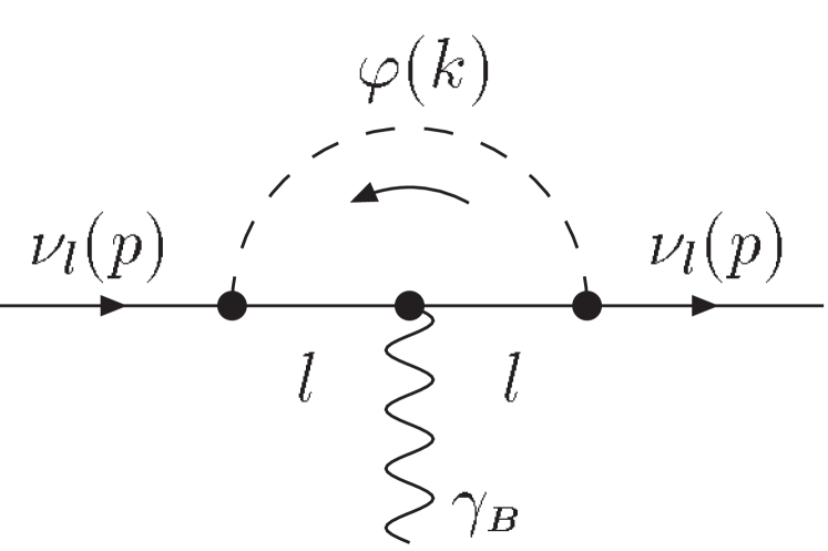
a

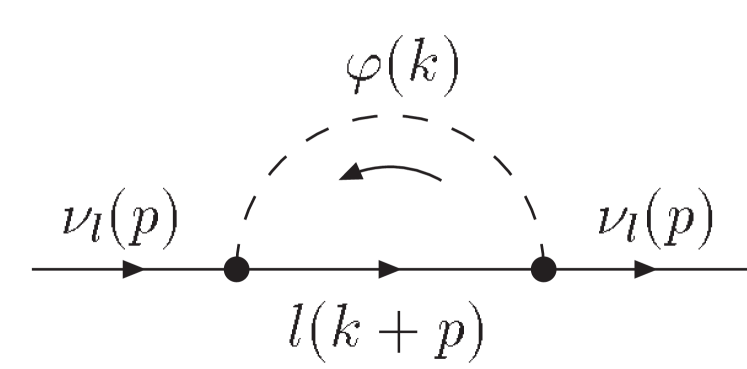
b

Figure 1: a) Neutrino vertex $\Lambda_{\mu}^{\varphi ll}(p,0,p)$. b) Neutrino self-energy ${\sum\nolimits}^{\varphi l}(p)$.

$$\Lambda_{\mu}^{\varphi ll}(p,0,p)=\frac{e^{3}m^{2}_{l}}{2s^{2}_{W}M^{2}_{W}}\int\frac{d^{4}k}{(2\pi)^{4}}\ \omega_{+}S_{F}(k+p)\gamma_{\mu}S_{F}(k+p)\Delta_{F}(k)\omega_{-}\,,$$ (2)

where the superscript labels the particles in the loop, $S_{F}(k+p)$ and $\Delta_{F}(k)$ are the propagators of the fermion and scalar field respectively, and the $\omega_{\pm}$ are the chirality projectors. Let us now consider the diagram shown in Fig. 1b. The self-energy is given by

$${\sum\nolimits}^{\varphi l}(p)=\frac{e^{2}m^{2}_{l}}{2s^{2}_{W}M^{2}_{W}}\int\frac{d^{4}k}{(2\pi)^{4}}\ \omega_{+}\Delta_{F}(k)S_{F}(k+p)\omega_{-}\ .$$ (3)

From Eq. (2) and (3) the identity

$$-\,e\ \frac{\partial{\sum\nolimits}^{\varphi l}(p)}{\partial p^{\mu}}=\Lambda_{\mu}^{\varphi ll}(p,0,p)\,,$$ (4)

follows. Similarly, the vertex of diagram 2a is given by

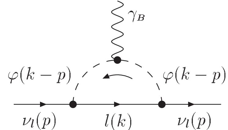
a

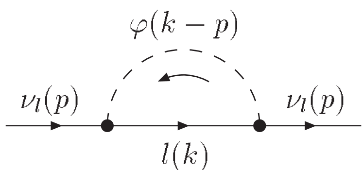
b

Figure 2: a) Neutrino vertex $\Lambda^{\varphi\varphi l}_{\mu}(p,0,p)$. b) Neutrino self-energy ${\sum\nolimits}^{\varphi l}(p)$.

$$\Lambda^{\varphi\varphi l}_{\mu}(p,0,p)=-\,\frac{e^{3}m_{l}^{2}}{2s^{2}_{W}M^{2}_{W}}\int\frac{d^{4}k}{(2\pi)^{4}}\ \omega_{+}\Delta_{F}(k-p)[2(k-p)_{\mu}]\Delta_{F}(k-p)S_{F}(k)\omega_{-}\,,$$ (5)

and the corresponding self-energy diagram 2b is

$${\sum\nolimits}^{\varphi l}(p)=\frac{e^{2}m^{2}}{2s^{2}_{W}M^{2}_{W}}\int\frac{d^{4}k}{(2\pi)^{4}}\ \omega_{+}\Delta_{F}(k-p)S_{F}(k)\omega_{-}\,,$$ (6)

so that they satisfy the identity

$$e\ \frac{\partial{\sum\nolimits}^{\varphi l}(p)}{\partial p^{\mu}}=\Lambda^{\varphi\varphi l}_{\mu}(p,0,p)\,.$$ (7)

Considering Eqs. (4) and (7) we see that the contributions to the vertex function of diagrams 1a and 2a cancel each other. This is also the case in the $R_{\xi}^{L}$ gauge, where the diagrams shown in Fig. 1 and 2 (with the change $\gamma_{{\scriptscriptstyle B}}\rightarrow\gamma$) lead to relations similar to those of equations (4) and (7).

The other two diagrams that contribute to the vertex involve a $W$ internal line. For the vertex shown in Fig. 3a we obtain

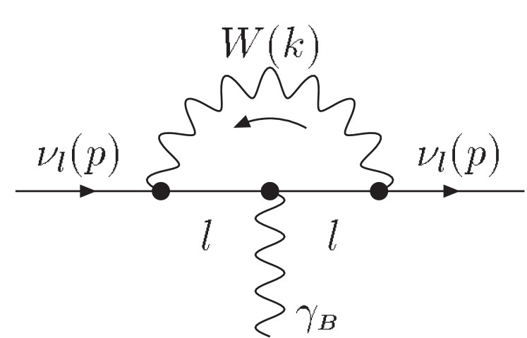
a

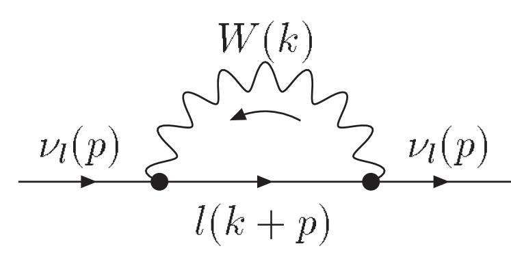
b

Figure 3: a) Neutrino vertex $\Lambda_{\mu}^{Wll}(p,0,p)$. b) Neutrino self-energy ${\sum\nolimits}^{Wl}(p)$.

$$\Lambda_{\mu}^{Wll}(p,0,p)=-\,\frac{e^{3}}{2s^{2}_{W}}\int\frac{d^{4}k}{(2\pi)^{4}}\ \gamma^{\alpha}\omega_{-}S_{F}(k+p)\gamma_{\mu}S_{F}(k+p)\gamma^{\beta}D^{W}_{\alpha\beta}(k)\omega_{-}\,,$$ (8)

where $D^{W}_{\alpha\beta}(k)$ is the propagator of the $W$ boson. The corresponding part of the self-energy of the neutrino (diagram 3b) is then

$${\sum\nolimits}^{Wl}(p)=-\,\frac{e^{2}}{2s^{2}_{W}}\int\frac{d^{4}k}{(2\pi)^{4}}\ \gamma^{\alpha}\omega_{-}D^{W}_{\alpha\beta}(k)\gamma^{\beta}S_{F}(k+p)\omega_{-}\,.$$ (9)

From Equations (8) and (9), it is straightforward to get the identity

$$-\,e\ \frac{\partial{\sum\nolimits}^{Wl}(p)}{\partial p^{\mu}}=\Lambda^{Wll}_{\mu}(p,0,p)\,,$$ (10)

which is a relation similar to that obtained in the $R_{\xi}^{L}$ gauge.

The last contribution to the proper vertex, Fig. 4a, involves the non Abelian vertex $\gamma_{{\scriptscriptstyle B}}WW$. It is given by

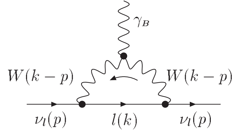
a

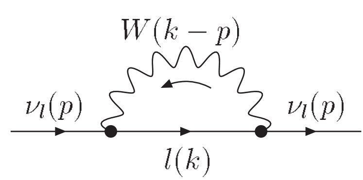
b

Figure 4: a) Neutrino vertex $\Lambda_{\mu}^{WWl}(p,0,p)$. b) Neutrino self-energy ${\sum\nolimits}^{Wl}(p)$.

$$\Lambda_{\mu}^{WWl}(p,0,p)=\frac{e^{2}}{2s^{2}_{W}}\int\frac{d^{4}k}{(2\pi)^{4}}\ \gamma^{\alpha}\omega_{-}\Gamma^{W\hat{A}W}_{\alpha\beta\mu}\,(k-p,0,k-p)\gamma^{\beta}S_{F}(k)\omega_{-}\,,$$ (11)

where we have defined

$$\Gamma^{W\hat{A}W}_{\alpha\beta\mu}\,(k-p,0,k-p)\equiv eD^{W}_{\alpha\alpha^{\prime}}(k-p)V^{W\hat{A}W}_{\alpha^{\prime}\beta^{\prime}\mu}[-(k-p),0,(k-p)]D^{W}_{\beta\beta^{\prime}}(k-p)\,,$$ (12)

with $V^{W\hat{A}W}_{\alpha\beta\mu}$ being the $\hat{A}WW$-coupling of a background field $\hat{A}$ with two W’s quantum fields (its explicit form can be found in Eqs. (A.33) and (A.34) of Ref. [11]). Using the contracted vertex $\Gamma^{W\hat{A}W}_{\alpha\beta\mu}$ defined in equation (12) it is possible to prove the WT identity

$$-\,e\ \frac{\partial D^{W}_{\alpha\beta}(l)}{\partial l^{\mu}}=\Gamma^{W\hat{A}W}_{\alpha\beta\mu}(l,0,l),$$ (13)

where $l=k-p$. This formula is crucial for the computation because it relates the quantum W’s fields with the background $\hat{A}$ field and can not be obtained by the usual derivative procedure of the functional generator. Equation (13) is formally the same as Eq. (5) in Ref. [15] for the non linear $R_{\xi}^{NL}$ gauge. The proof of this WT identity is given in Appendix A.

Taking now into account that the corresponding contribution to the self-energy (diagram 4b) is

$${\sum\nolimits}^{Wl}(p)=-\,\frac{e^{2}}{2s^{2}_{W}}\int\frac{d^{4}k}{(2\pi)^{4}}\ \gamma^{\alpha}\,\omega_{-}D^{W}_{\alpha\beta}(k-p)\gamma^{\beta}S_{F}(k)\omega_{-}\,,$$ (14)

with the help of the WT identity (13), it is easy to prove the relation

$$e\ \frac{\partial{\sum\nolimits}^{Wl}(p)}{\partial p^{\mu}}=\Lambda^{WWl}_{\mu}\,(p,0,p)\,,$$ (15)

so that the contributions of diagrams 3 and 4 cancel each other again. The relation shown in Eq. (15) doesn’t exist in the linear $R_{\xi}^{L}$ gauge.

With only these four diagrams the cancellation of the NEC is not obtained in the $R_{\xi}^{L}$ gauge. There are two additional diagrams involving the $\gamma W\varphi$ vertex plus one improper diagram (transverse part of $\gamma Z$ self-energy) that should be considered. Only then one obtains [17] ${\cal Q}_{\nu}^{{\scriptscriptstyle R^{L}_{\xi}}}=0$, in an obvious notation. In the BFM the last self-energy also exists, but its contribution to the NEC vanishes [see Eq. (34) in Ref. [11]] because the transverse part of the $\gamma_{{\scriptscriptstyle B}}Z_{\scriptscriptstyle B}$ self-energy is zero.

In the BFM the four proper vertices at zero momentum transfer, satisfy the relation

$$\Lambda^{\varphi ll}_{\mu}+\Lambda^{\varphi\varphi l}_{\mu}+\Lambda^{Wll}_{\mu}+\Lambda^{WWl}_{\mu}=0\,,$$ (16)

which implies the vanishing of the NEC,

$${\cal Q}_{\nu}^{{\scriptscriptstyle BFM}}=F_{{\scriptscriptstyle NEC}}^{{\scriptscriptstyle BFM}}\Big{(}0,\xi_{Q}^{W}\Big{)}=0\,.$$ (17)

The proof of the exactly cancellation of the electro-magnetic proper neutrino vertex at one-loop, is a consequence of the most general WT identity (see Eq. (36) in the Ref. [11]) valid to all orders in perturbation theory.

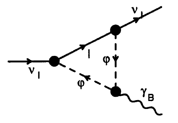
a

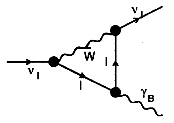
b

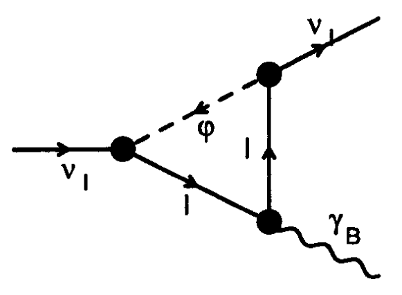
c

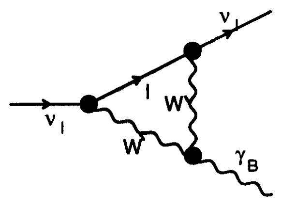
d

Figure 5: Vertex contributions to the NEC and NMM in the BFM.

3 Neutrino Electric Charge, Explicit Calculation

In this section we present a complete calculation of the neutrino electric charge using: a) the BFM and b) the usual formulation in the linear $R_{\xi}^{L}$ gauge . In both cases the calculation is done for arbitrary $q^{2}$ of the photon and carrying all the gauge dependence on the $\xi$ parameter [18, 19]. Cancellation of the gauge dependence, in the $q^{2}\rightarrow 0$ limit, will be explicitly shown, using an expansion of the different contributions to the Dirac form factor around $q^{2}=0$.

3.1 Calculation in the BFM

The proper diagrams contributing to the NEC are given in Fig. 5. Using the Feynman rules of the electroweak BFM [11] and after some algebra one finds for the Dirac form factor defined in Eq. (1), at $q^{2}=0$, the following contributions:

$$\begin{array}[]{c}\displaystyle{\cal Q}_{\nu_{l}}\Big{|}_{{\scriptscriptstyle Fig.5a}}^{{\scriptscriptstyle BFM}}=F^{{\scriptscriptstyle BFM}}_{{\scriptscriptstyle NEC}}\Big{(}q^{2}=0,\xi_{Q}^{W}\Big{)}\Big{|}_{{\scriptscriptstyle Fig.5a}}=-\frac{\alpha em_{l}^{2}}{64\pi M_{W}^{2}s_{W}^{2}\Big{(}M_{W}^{2}-m_{l}^{2}\xi_{Q}^{W}\Big{)}^{2}}\times\\[19.91684pt] \displaystyle\Bigg{\{}\Big{(}M_{W}^{2}-m_{l}^{2}\xi_{Q}^{W}\Big{)}\Big{(}M_{W}^{2}-3m_{l}^{2}\xi_{Q}^{W}\Big{)}+2\Big{(}\xi_{Q}^{W}\Big{)}^{2}m_{l}^{4}B_{0}\,(0;m_{l}^{2},m_{l}^{2})\\[19.91684pt] \displaystyle+2M_{W}^{2}\Big{(}M_{W}^{2}-2m_{l}^{2}\xi_{Q}^{W}\Big{)}B_{0}\Bigg{(}0;\frac{M^{2}_{W}}{\xi_{Q}^{W}},\frac{M^{2}_{W}}{\xi_{Q}^{W}}\Bigg{)}\Bigg{\}}\ ;\end{array}$$ (18)

$${\cal Q}_{\nu_{l}}\Big{|}_{{\scriptscriptstyle Fig.5b}}^{{\scriptscriptstyle BFM}}=F^{{\scriptscriptstyle BFM}}_{{\scriptscriptstyle NEC}}\Big{(}q^{2}=0,\xi_{Q}^{W}\Big{)}\Big{|}_{{\scriptscriptstyle Fig.5b}}=-\frac{\alpha e}{32\pi(m_{l}^{2}-M_{W}^{2})^{2}s_{W}^{2}\xi_{Q}^{W}\Big{(}M_{W}^{2}-m_{l}^{2}\xi_{Q}^{W}\Big{)}^{2}}\times$$

$$\Bigg{\{}3M_{W}^{2}m_{l}^{2}\xi_{Q}^{W}\Big{(}M_{W}^{2}-m_{l}^{2}\xi_{Q}^{W}\Big{)}^{2}B_{0}\,(0;M_{W}^{2},M_{W}^{2})$$

$$+m_{l}^{4}\xi_{Q}^{W}\Big{[}-2\xi_{Q}^{W}m_{l}^{4}+M_{W}^{2}\Big{(}-3\Big{(}\xi_{Q}^{W}\Big{)}^{2}+4\xi_{Q}^{W}+3\Big{)}m_{l}^{2}+2M_{W}^{4}\Big{(}2\xi_{Q}^{W}-3\Big{)}\Big{]}B_{0}\,(0;m_{l}^{2},m_{l}^{2})$$

$$-M_{W}^{2}\Big{(}2M_{W}^{2}-m_{l}^{2}\xi_{Q}^{W}\Big{)}(m_{l}^{2}-M_{W}^{2})^{2}B_{0}\Bigg{(}0;\frac{M^{2}_{W}}{\xi_{Q}^{W}},\frac{M^{2}_{W}}{\xi_{Q}^{W}}\Bigg{)}$$

$$-\Big{[}-\xi_{Q}^{W}m_{l}^{4}+M_{W}^{2}\Big{(}-3\Big{(}\xi_{Q}^{W}\Big{)}^{2}+\xi_{Q}^{W}+2\Big{)}m_{l}^{2}+M_{W}^{4}\Big{(}3\xi_{Q}^{W}-2\Big{)}\Big{]}(m_{l}^{2}-M_{W}^{2})\Big{(}M_{W}^{2}-m_{l}^{2}\xi_{Q}^{W}\Big{)}\Bigg{\}}\ ;$$ (19)

$${\cal Q}_{\nu_{l}}\Big{|}_{{\scriptscriptstyle Fig.5c}}^{{\scriptscriptstyle BFM}}=F^{{\scriptscriptstyle BFM}}_{{\scriptscriptstyle NEC}}\Big{(}q^{2}=0,\xi_{Q}^{W}\Big{)}\Big{|}_{{\scriptscriptstyle Fig.5c}}=-{\cal Q}_{\nu_{l}}\Big{|}_{{\scriptscriptstyle Fig.5a}}^{{\scriptscriptstyle BFM}}\,;$$ (20)

$${\cal Q}_{\nu_{l}}\Big{|}_{{\scriptscriptstyle Fig.5d}}^{{\scriptscriptstyle BFM}}=F^{{\scriptscriptstyle BFM}}_{{\scriptscriptstyle NEC}}\Big{(}q^{2}=0,\xi_{Q}^{W}\Big{)}\Big{|}_{{\scriptscriptstyle Fig.5d}}=-{\cal Q}_{\nu_{l}}\Big{|}_{{\scriptscriptstyle Fig.5b}}^{{\scriptscriptstyle BFM}}\ .$$ (21)

Notice that we have kept explicitly the gauge dependence in all equations. From Eqs. (18-21) it obviously follows that the NEC vanishes,

$${\cal Q}_{\nu_{l}}^{{\scriptscriptstyle BFM}}={\cal Q}_{\nu_{l}}\Big{|}_{{\scriptscriptstyle Fig.5a}}^{{\scriptscriptstyle BFM}}+{\cal Q}_{\nu_{l}}\Big{|}_{{\scriptscriptstyle Fig.5b}}^{{\scriptscriptstyle BFM}}+{\cal Q}_{\nu_{l}}\Big{|}_{{\scriptscriptstyle Fig.5c}}^{{\scriptscriptstyle BFM}}+{\cal Q}_{\nu_{l}}\Big{|}_{{\scriptscriptstyle Fig.5d}}^{{\scriptscriptstyle BFM}}=0,$$ (22)

in agreement with the result (17), obtained using the Ward-Takahashi identity.

Expressions (18-21) have been obtained applying a Taylor expansion, around $q^{2}=0$, to the complete contribution of each diagram. The complete contribution of all diagrams to the $F^{{\scriptscriptstyle BFM}}_{{\scriptscriptstyle NEC}}\Big{(}q^{2},\xi_{Q}^{W}\Big{)}$ form factor is given in [20]. To obtain these formulae we have made use of the new relations between scalar three point function, $C_{0}$, and two point functions $B_{0}$, given in Appendix B.

With these formulae it is easy to prove for the complete form factor that again

$${\cal Q}_{\nu_{l}}^{{\scriptscriptstyle BFM}}=\lim_{q^{2}\rightarrow 0}F^{{\scriptscriptstyle BFM}}_{{\scriptscriptstyle NEC}}\Big{(}q^{2},\xi_{Q}^{W}\Big{)}=0\ .$$ (23)

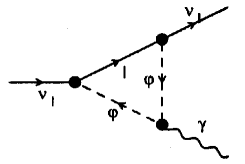
a

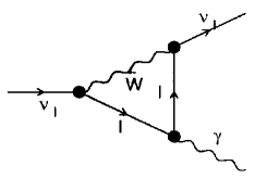
b

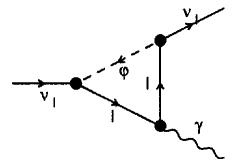
c

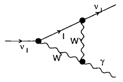
d

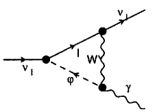
e

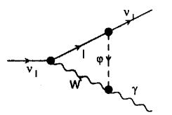
f

Figure 6: Vertex contributions to the NEC and NMM in the linear $R_{\xi}^{L}$ gauge.

3.2 Calculation in the linear $R_{\xi}^{L}$ gauge

The proper vertices contributing to the NEC in the linear $R_{\xi}^{L}$ gauge are those given in Fig. 6. Notice that there are two diagrams that do not appear in the BFM. A procedure similar to that used in the previous subsection leads to the following result:

$${\cal Q}_{\nu_{l}}\Big{|}_{{\scriptscriptstyle Fig.6a}}^{{\scriptscriptstyle R_{\xi}^{L}}}=F^{{\scriptscriptstyle R_{\xi}^{L}}}_{{\scriptscriptstyle NEC}}(q^{2}=0,\xi_{W})\Big{|}_{{\scriptscriptstyle Fig.6a}}=F^{{\scriptscriptstyle BFM}}_{{\scriptscriptstyle NEC}}\Big{(}q^{2}=0,\xi_{Q}^{W}\rightarrow\xi_{W}\Big{)}\Big{|}_{{\scriptscriptstyle Fig.5a}}\ ;$$ (24)

$${\cal Q}_{\nu_{l}}\Big{|}_{{\scriptscriptstyle Fig.6b}}^{{\scriptscriptstyle R_{\xi}^{L}}}=F^{{\scriptscriptstyle R_{\xi}^{L}}}_{{\scriptscriptstyle NEC}}(q^{2}=0,\xi_{W})\Big{|}_{{\scriptscriptstyle Fig.6b}}=F^{{\scriptscriptstyle BFM}}_{{\scriptscriptstyle NEC}}\Big{(}q^{2}=0,\xi_{Q}^{W}\rightarrow\xi_{W}\Big{)}\Big{|}_{{\scriptscriptstyle Fig.5b}}\ ;$$ (25)

$${\cal Q}_{\nu_{l}}\Big{|}_{{\scriptscriptstyle Fig.6c}}^{{\scriptscriptstyle R_{\xi}^{L}}}=F^{{\scriptscriptstyle R_{\xi}^{L}}}_{{\scriptscriptstyle NEC}}(q^{2}=0,\xi_{W})\Big{|}_{{\scriptscriptstyle Fig.6c}}=F^{{\scriptscriptstyle BFM}}_{{\scriptscriptstyle NEC}}\Big{(}q^{2}=0,\xi_{Q}^{W}\rightarrow\xi_{W}\Big{)}\Big{|}_{{\scriptscriptstyle Fig.5c}}\ ;$$ (26)

$${\cal Q}_{\nu_{l}}\Big{|}_{{\scriptscriptstyle Fig.6d}}^{{\scriptscriptstyle R_{\xi}^{L}}}=F^{{\scriptscriptstyle R_{\xi}^{L}}}_{{\scriptscriptstyle NEC}}(q^{2}=0,\xi_{W})\Big{|}_{{\scriptscriptstyle Fig.6d}}=$$

$$\frac{\alpha e}{64\pi(m_{l}^{2}-M_{W}^{2})^{2}s_{W}^{2}(M_{W}^{2}-m_{l}^{2}\xi_{W})(1-\xi_{W})\xi_{W}}\times$$

$$\Bigg{\{}[5m_{l}^{2}(\xi_{W}+1)+M_{W}^{2}(\xi_{W}-5)](m_{l}^{2}-M_{W}^{2})(M_{W}^{2}-m_{l}^{2}\xi_{W})(1-\xi_{W})$$

$$+\,6[m_{l}^{2}(1+\xi_{W})-2M_{W}^{2}]m_{l}^{4}(1-\xi_{W})\xi_{W}B_{0}\,(0;m_{l}^{2},m_{l}^{2})$$

$$+\,6[m_{l}^{2}(1-2\xi_{W})+M_{W}^{2}\xi_{W}]M_{W}^{2}(M_{W}^{2}-m_{l}^{2}\xi_{W})\xi_{W}B_{0}\,(0;M_{W}^{2},M_{W}^{2})$$

$$-\,6M_{W}^{2}(m_{l}^{2}-M_{W}^{2})^{2}B_{0}\Bigg{(}0;\frac{M^{2}_{W}}{\xi_{W}},\frac{M^{2}_{W}}{\xi_{W}}\Bigg{)}\Bigg{\}}\ ;$$ (27)

$${\cal Q}_{\nu_{l}}\Big{|}_{{\scriptscriptstyle Fig.6e}}^{{\scriptscriptstyle R_{\xi}^{L}}}=F^{{\scriptscriptstyle R_{\xi}^{L}}}_{{\scriptscriptstyle NEC}}(q^{2}=0,\xi_{W})\Big{|}_{{\scriptscriptstyle Fig.6e}}=$$

$${\cal Q}_{\nu_{l}}\Big{|}_{{\scriptscriptstyle Fig.6f}}^{{\scriptscriptstyle R_{\xi}^{L}}}=F^{{\scriptscriptstyle R_{\xi}^{L}}}_{{\scriptscriptstyle NEC}}(q^{2}=0,\xi_{W})\Big{|}_{{\scriptscriptstyle Fig.6f}}$$

$$=\frac{\alpha e}{64\pi(m_{l}^{2}-M_{W}^{2})s_{W}^{2}(M_{W}^{2}-m_{l}^{2}\xi_{W})^{2}(1-\xi_{W})}\times$$

$$\Bigg{\{}-\,m_{l}^{2}(m_{l}^{2}-M_{W}^{2})(M_{W}^{2}-m_{l}^{2}\xi_{W})(1-\xi_{W})$$

$$+\,\xi_{W}[m_{l}^{2}(3\xi_{W}+1)-4M_{W}^{2}]m_{l}^{4}(1-\xi_{W})B_{0}\,(0;m_{l}^{2},m_{l}^{2})$$

$$+3\xi_{W}m_{l}^{2}(M_{W}^{2}-m_{l}^{2}\xi_{W})^{2}B_{0}(0;M^{2}_{W},M^{2}_{W})$$

$$+\,\xi_{W}[m_{l}^{2}(2\xi_{W}+1)-3M_{W}^{2}]m_{l}^{2}(m_{l}^{2}-M_{W}^{2})B_{0}\Bigg{(}0;\frac{M^{2}_{W}}{\xi_{W}},\frac{M^{2}_{W}}{\xi_{W}}\Bigg{)}\Bigg{\}}\ .$$ (28)

Therefore, as in the BFM, the contributions from the diagrams 6a and 6c cancel each other, but the sum of the contributions of the diagrams 6b, 6d, 6e and 6f does not vanish. However, there exists an important relation between BFM and $R_{\xi}^{L}$ gauge

$$\begin{array}[]{c}\displaystyle F^{{\scriptscriptstyle BFM}}_{{\scriptscriptstyle NEC}}\Big{(}q^{2}=0,\xi_{Q}^{W}\rightarrow\xi_{W}\Big{)}\Big{|}_{{\scriptscriptstyle Fig.5d}}=F^{{\scriptscriptstyle R_{\xi}^{L}}}_{{\scriptscriptstyle NEC}}(q^{2}=0,\xi_{W})\Big{|}_{{\scriptscriptstyle Fig.6d}}\\[19.91684pt] \displaystyle+\,F^{{\scriptscriptstyle R_{\xi}^{L}}}_{{\scriptscriptstyle NEC}}(q^{2}=0,\xi_{W})\Big{|}_{{\scriptscriptstyle Fig.6e}}+\,F^{{\scriptscriptstyle R_{\xi}^{L}}}_{{\scriptscriptstyle NEC}}(q^{2}=0,\xi_{W})\Big{|}_{{\scriptscriptstyle Fig.6f}}+{\sum\nolimits}_{\gamma Z}^{{\scriptscriptstyle R_{\xi}^{L}}}\end{array}$$ (29)

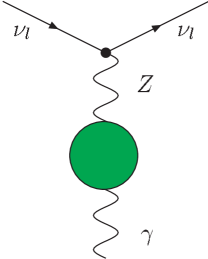
Figure 7: Improper vertex contribution to the NEC in the linear $R_{\xi}^{L}$ gauge.

where ${\sum\nolimits}_{\gamma Z}^{{\scriptscriptstyle R_{\xi}^{L}}}$ is the bosonic contribution of the transverse part of the $\gamma Z$ self-energy (improper vertex) [17, 21], shown in Fig. 7 . This self-energy is computed in [20] for arbitrary $q^{2}$ and, from there, we obtain

$$\begin{array}[]{c}\displaystyle{\sum\nolimits}_{\gamma Z}^{{\scriptscriptstyle R_{\xi}^{L}}}=\frac{e{\sum\nolimits}_{T}^{\gamma Z}(q^{2}=0,\xi_{W})}{4s_{W}c_{W}M_{Z}^{2}}=\frac{\alpha e}{64\pi s^{2}_{W}\xi_{W}(1-\xi_{W})}\times\\[19.91684pt] \displaystyle\Bigg{\{}(5\xi_{W}+1)(1-\xi_{W})-6\xi_{W}^{2}B_{0}(0;M^{2}_{W},M_{W}^{2})+2(2\xi_{W}+1)B_{0}\Bigg{(}0;\frac{M^{2}_{W}}{\xi_{W}},\frac{M^{2}_{W}}{\xi_{W}}\Bigg{)}\Bigg{\}}\ .\end{array}$$ (30)

Summing up all these contributions one get an equation for the NEC which is formally the same as that given in Eq. (22), so that

$$\begin{array}[]{c}\displaystyle{\cal Q}_{\nu_{l}}^{{\scriptscriptstyle R_{\xi}^{L}}}={\cal Q}_{\nu_{l}}\Big{|}_{{\scriptscriptstyle Fig.6a}}^{{\scriptscriptstyle R_{\xi}^{L}}}+{\cal Q}_{\nu_{l}}\Big{|}_{{\scriptscriptstyle Fig.6b}}^{{\scriptscriptstyle R_{\xi}^{L}}}+{\cal Q}_{\nu_{l}}\Big{|}_{{\scriptscriptstyle Fig.6c}}^{{\scriptscriptstyle R_{\xi}^{L}}}\\[19.91684pt] \displaystyle+{\cal Q}_{\nu_{l}}\Big{|}_{{\scriptscriptstyle Fig.6d}}^{{\scriptscriptstyle R_{\xi}^{L}}}+{\cal Q}_{\nu_{l}}\Big{|}_{{\scriptscriptstyle Fig.6e}}^{{\scriptscriptstyle R_{\xi}^{L}}}+{\cal Q}_{\nu_{l}}\Big{|}_{{\scriptscriptstyle Fig.6f}}^{{\scriptscriptstyle R_{\xi}^{L}}}+{\sum\nolimits}_{\gamma Z}^{{\scriptscriptstyle R_{\xi}^{L}}}=0\ .\end{array}$$ (31)

4 Neutrino Magnetic Moment

4.1 Computation in the BFM and the linear $R_{\xi}^{L}$ gauge

In the minimal extension of the Standard Model (SM), in which a right handed neutrino for each family is added, a neutrino magnetic moment (NMM) arises naturally. We shall compute it here, both in the BFM and the $R_{\xi}^{L}$ gauge, considering massive Dirac neutrinos with no flavor mixing [22]. It is given by the Pauli form factor of Eq. (1),

$${\mu}_{\nu_{l}}=\lim_{q^{2}\rightarrow 0}F^{{\scriptscriptstyle BFM;R_{\xi}^{L}}}_{{\scriptscriptstyle NMM}}(q^{2},m_{\nu_{l}},\xi)\ .$$ (32)

As in the previous section the contributing diagrams are given in Fig. 5 for the BFM and in Fig. 6 for the linear $R_{\xi}^{L}$ gauge. We thus obtain

$$\mu_{\nu_{l}}\big{|}_{{\scriptscriptstyle Fig.5a}}^{{\scriptscriptstyle BFM}}=\mu_{\nu_{l}}\Big{|}_{{\scriptscriptstyle Fig.6a}}^{{\scriptscriptstyle R_{\xi}^{L}}}=\frac{em_{\nu_{l}}G_{{\scriptscriptstyle F}}}{4\pi^{2}\sqrt{2}}\Bigg{\{}\frac{5{\xi}}{12}x+\cdots\Bigg{\}}\ ,$$ (33)

$$\mu_{\nu_{l}}\big{|}_{{\scriptscriptstyle Fig.5b}}^{{\scriptscriptstyle BFM}}=\mu_{\nu_{l}}\Big{|}_{{\scriptscriptstyle Fig.6b}}^{{\scriptscriptstyle R_{\xi}^{L}}}=\frac{em_{\nu_{l}}G_{{\scriptscriptstyle F}}}{4\pi^{2}\sqrt{2}}\Bigg{\{}\frac{2}{3}+x\Bigg{[}\frac{5{\xi}}{3}-\frac{1}{2}+{\xi}\Big{(}\log x+\log{\xi}\Big{)}\Bigg{]}+\cdots\Bigg{\}}\ ,$$ (34)

$$\mu_{\nu_{l}}\big{|}_{{\scriptscriptstyle Fig.5c}}^{{\scriptscriptstyle BFM}}=\mu_{\nu_{l}}\Big{|}_{{\scriptscriptstyle Fig.6c}}^{{\scriptscriptstyle R_{\xi}^{L}}}=\frac{em_{\nu_{l}}G_{{\scriptscriptstyle F}}}{4\pi^{2}\sqrt{2}}\Bigg{\{}-x{\xi}\Bigg{[}\frac{5}{3}+\log x+\log{\xi}\Bigg{]}+\cdots\Bigg{\}}\ ,$$ (35)

$$\mu_{\nu_{l}}\Big{|}_{{\scriptscriptstyle Fig.6d}}^{{\scriptscriptstyle R_{\xi}^{L}}}=\frac{em_{\nu_{l}}G_{{\scriptscriptstyle F}}}{4\pi^{2}\sqrt{2}}\Bigg{\{}\frac{1}{12}\Big{(}7-5x{\xi}\Big{)}+\cdots\Bigg{\}}\ ,$$ (36)

$$\mu_{\nu_{l}}\Big{|}_{{\scriptscriptstyle Fig.6e}}^{{\scriptscriptstyle R_{\xi}^{L}}}=\mu_{\nu_{l}}\Big{|}_{{\scriptscriptstyle Fig.6f}}^{{\scriptscriptstyle R_{\xi}^{L}}}=\frac{em_{\nu_{l}}G_{{\scriptscriptstyle F}}}{4\pi^{2}\sqrt{2}}\Bigg{\{}\frac{1}{8}\Big{(}1-x\Big{)}+\cdots\Bigg{\}}\ ,$$ (37)

$$\mu_{\nu_{l}}\big{|}_{{\scriptscriptstyle Fig.5d}}^{{\scriptscriptstyle BFM}}=\mu_{\nu_{l}}\Big{|}_{{\scriptscriptstyle Fig.6d}}^{{\scriptscriptstyle R_{\xi}^{L}}}+\mu_{\nu_{l}}\Big{|}_{{\scriptscriptstyle Figs.6e+6f}}^{{\scriptscriptstyle R_{\xi}^{L}}}=\frac{em_{\nu_{l}}G_{{\scriptscriptstyle F}}}{4\pi^{2}\sqrt{2}}\Bigg{\{}\frac{5}{6}-x\Bigg{[}\frac{1}{4}+\frac{5{\xi}}{12}\Bigg{]}+\cdots\Bigg{\}}\ ,$$ (38)

where $G_{F}$ is the Fermi constant, $x=m_{l}^{2}/M^{2}_{W}$ and the expressions are given up to second order in the $x$ expansion. As we can see, the contributions from diagrams 5a, 5b and 5c are the same in the BFM and in the linear $R_{\xi}^{L}$ gauge (just by changing $\xi_{Q}^{W}\rightarrow\xi_{W}$), and the sum of the contributions of diagrams 6d, 6e and 6f is equal to the contribution of figure 5d (with the same substitution in the gauge parameter). The dependence in the gauge parameter $\xi$ is explicitly shown in the formulae. The cancellation of the gauge parameter is then obtained after summing up all contributions. However, to leading (first) order in $m_{\nu}$, each diagram separately is finite, as well as gauge parameter and gauge structure (linear or not linear) independent. In this limit we recover the well know expression of the neutrino magnetic moment (NMM) [23]

$$\mu_{\nu_{l}}=\frac{3em_{\nu_{l}}G_{{\scriptscriptstyle F}}}{8\pi^{2}\sqrt{2}}\ .$$ (39)

Even in the $R_{\xi}^{L}$ gauge, there are no contributions to the magnetic anomaly coming from the $\gamma Z$ self-energy.

The exact expressions for the form factor $F_{{\scriptscriptstyle NMM}}^{{\scriptscriptstyle BFM;R_{\xi}^{L}}}(m_{\nu_{l}},{\xi})$ (at $q^{2}=0$) to all orders in x is given in [20]. From there and using the relations of Appendix B one gets the exact expression

$$\begin{array}[]{c}\displaystyle F_{{\scriptscriptstyle NMM}}^{{\scriptscriptstyle BFM;R_{\xi}^{L}}}(m_{\nu_{l}})=\frac{\alpha e}{4\pi}\frac{3m_{\nu_{l}}}{4s^{2}_{W}(m_{l}^{2}-M_{W}^{2})^{2}}\times\\[19.91684pt] \displaystyle\Bigg{\{}\frac{m_{l}^{4}-5m_{l}^{2}M_{W}^{4}+2M_{W}^{4}}{2M_{W}^{2}}+\frac{m_{l}^{4}[B_{0}(0;M^{2}_{W},M^{2}_{W})-B_{0}\,(0;m_{l}^{2},m_{l}^{2})]}{m_{l}^{2}-M_{W}^{2}}\Bigg{\}}\ ,\end{array}$$ (40)

where the cancellation of the gauge dependence has been made evident. Using now the expression of the scalar two point function, $B_{0}$, one gets [22]

$$F_{{\scriptscriptstyle NMM}}^{{\scriptscriptstyle BFM;R_{\xi}^{L}}}(m_{\nu_{l}})=-\frac{em_{\nu_{l}}G_{{\scriptscriptstyle F}}}{4\pi^{2}\sqrt{2}}\Bigg{\{}\frac{3[x^{3}+2(\log x-3)x^{2}+7x-2]}{4(1-x)^{3}}\Bigg{\}}\ ,$$ (41)

that at leading order in $x$ coincides with Eq. (39).

5 Conclusions

We have calculated the neutrino electric charge in the background field method and in the linear $R_{\xi}^{L}$ gauge for arbitrary values of the gauge fixing parameters. In the BFM it has been obtained in two different ways: a) making use of the usual Ward-Takahashi identities for self-energy and vertex one loop diagrams in addition to a new one, deduced for the non Abelian vertex of a background field $\hat{A}$ and two quantum W’s fields ($W{\hat{A}}W$); and b) by computing explicitly the contributing diagrams and checking in this way the WT identities. In the linear $R_{\xi}^{L}$ gauge more diagrams have to be taken into account, including the improper vertex. Therefore the BFM enjoys the simplicity of theories with nonlinear gauge fixing terms: fewer diagrams and simple WT identities. We have found that, as expected, both methods lead to the same result, namely: the neutrino electric charge vanishes.

For Dirac massive neutrinos, we have calculated the magnetic moment in both BFM and $R_{\xi}^{L}$ gauge, reproducing known results at leading order in $(\frac{m_{1}}{M_{W}})$. We have established the diagrammatic correspondence between the two methods and the gauge parameter cancellations. Finally, we showed its gauge parameter and gauge structure independence explicitly.

Appendix A. Ward Takahashi identity with a
background photon and two W’s quantum fields

When the momentum of the background photon is zero, the vertex can be written as [see Eqs. (A.33) from Ref. [11]]

$$V_{\alpha^{\prime}\beta^{\prime}\mu}^{W\hat{A}W}(-l,0,l)=-ie\Big{[}-2l_{\mu}g_{\alpha^{\prime}\beta^{\prime}}+\Big{(}1-\xi_{Q}^{W}\Big{)}g_{\mu\alpha^{\prime}}l_{\beta^{\prime}}+\Big{(}1-\xi_{Q}^{W}\Big{)}g_{\beta^{\prime}\mu}l_{\alpha^{\prime}}\Big{]}\,.\\$$

Contracting the vertex tensor (A.1) with the $W^{\prime}s$ quantum propagators we get

$$\Gamma_{\alpha\beta\mu}^{W\hat{A}W}(l,0,l)=e\,\left\{\frac{\Big{(}1-\xi_{Q}^{W}\Big{)}\,(g_{\mu\alpha}l_{\beta}+g_{\beta\mu}l_{\alpha})-2g_{\alpha\beta}l_{\mu}}{\Big{(}l^{2}-M^{2}_{W}\Big{)}^{2}}\right.$$

$$-\frac{\Big{(}1-\xi_{Q}^{W}\Big{)}\theta l^{2}(g_{\alpha\mu}l_{\beta}+g_{\mu\beta}l_{\alpha})}{\Big{(}l^{2}-M^{2}_{W}\Big{)}^{2}\Big{(}l^{2}-\frac{M^{2}_{W}}{\xi_{Q}^{W}}\Big{)}}+\frac{4\theta l_{\alpha}l_{\beta}l_{\mu}}{\Big{(}l^{2}-M^{2}_{W}\Big{)}^{2}\Big{(}l^{2}-\frac{M^{2}_{W}}{\xi_{Q}^{W}}\Big{)}}$$

$$\left.-\frac{2\Big{(}1-\xi_{Q}^{W}\Big{)}\theta l_{\alpha}l_{\beta}l_{\mu}}{\Big{(}l^{2}-M_{W}^{2}\Big{)}^{2}\Big{(}l^{2}-\frac{M^{2}_{W}}{\xi_{Q}^{W}}\Big{)}}-\frac{2\xi_{Q}^{W}\theta^{2}l^{2}l_{\alpha}l_{\beta}l_{\mu}}{\Big{(}l^{2}-M_{W}^{2}\Big{)}^{2}\Big{(}l^{2}-\frac{M^{2}_{W}}{\xi_{Q}^{W}}\Big{)}^{2}}\right\},$$

where we have defined

$$\theta\equiv 1-\frac{1}{\xi_{Q}^{W}}.\\$$

On the other hand, the derivative of the boson propagator $W$ is

$$-e\,\frac{\partial D^{W}_{\alpha\beta}(l)}{\partial l^{\mu}}=e\,\left\{\frac{-\theta(l_{\alpha}g_{\mu\beta}+l_{\beta}g_{\mu\alpha})}{\Big{(}l^{2}-M^{2}_{W}\Big{)}\Big{(}l^{2}-\frac{M^{2}_{W}}{\xi_{Q}^{W}}\Big{)}}-\frac{2l_{\mu}g_{\alpha\beta}}{\Big{(}l^{2}-M^{2}_{W}\Big{)}^{2}}\right.$$

$$+\left.\frac{2\theta l_{\alpha}l_{\beta}l_{\mu}}{(l^{2}-M^{2}_{W})\Big{(}l^{2}-\frac{M^{2}_{W}}{\xi_{Q}^{W}}\Big{)}}\left[\frac{1}{\Big{(}l^{2}-M^{2}_{W}\Big{)}}+\frac{1}{\Big{(}l^{2}-\frac{M^{2}_{W}}{\xi_{Q}^{W}}\Big{)}}\right]\right\}\,,\\$$

so that the comparison of (A.2) and (A.4) gives

$$-e\,\frac{\partial D^{W}_{\alpha\beta}(l)}{\partial l^{\mu}}=\Gamma^{W\hat{A}W}_{\alpha\beta\mu}(l,0,l)\,.\\$$

Appendix B. Scalar one loop integrals.

We present in this Appendix all the scalar one-loop integrals that we encountered in the calculation of the NEC and NMM [24, 25]. The one-loop integrals $A_{0},B_{0}$ and $C_{0}$ are not independent in special kinematical situations [21, 26, 27, 28].

$\bullet$ One-point function:

$$A_{0}(m^{2})=m^{2}\Bigg{(}\Delta-\log\frac{m^{2}}{\mu^{2}}+1\Bigg{)}\ \ with\ \ \Delta=\frac{2}{\epsilon}-\gamma_{E}+\log 4\pi\ ,\\$$

and where $\gamma_{E}$ is the Euler-Mascheroni’s constant.

$\bullet$ Two-point functions:

$$B_{0}(0;m^{2},m^{2})=\Delta-\log\frac{m^{2}}{\mu^{2}}\ \ ;\ \ B_{0}(0;0,m^{2})=B_{0}(0;m^{2},m^{2})+1\quad;$$

$$B_{0}(0;0,m^{2})=B_{0}(m^{2};0,m^{2})-1\ \ \ ;\ \ \quad A_{0}(m^{2})=m^{2}B_{0}(0;0,m^{2})\ ;$$

$$B_{0}(m^{2};0,m^{2})=B_{0}(0;m^{2},m^{2})+2\ \ ;\ \ A_{0}(m^{2})=m^{2}[1+B_{0}(0;m^{2},m^{2})]\ ;$$

$$(m_{1}^{2}-m_{2}^{2})B_{0}(0;m_{1}^{2},m_{2}^{2})=A_{0}(m_{1}^{2})-A_{0}(m_{2}^{2})\,;$$

$$B_{0}(q^{2};m_{1}^{2},m_{2}^{2})=B_{0}(0;m_{1}^{2},m_{2}^{2})$$

$$\,+\frac{q^{2}}{2(m_{1}^{2}-m_{2}^{2})^{2}}\Big{\{}(m_{1}^{2}+m_{2}^{2})[1+B_{0}(0,m_{1}^{2},m_{2}^{2})]-[A_{0}(m_{1}^{2})+A_{0}(m_{2}^{2})]\Big{\}}$$

$$+\,\frac{q^{4}}{6(m_{1}^{2}-m_{2}^{2})^{4}}\Bigg{\{}m_{1}^{4}+10m_{1}^{2}m_{2}^{2}+m_{2}^{4}$$

$$+\,3(m_{1}^{2}+m_{2}^{2})\Big{\{}(m_{1}^{2}+m_{2}^{2})B_{0}(0;m_{1}^{2},m_{2}^{2})-[A_{0}(m_{1}^{2})+A_{0}(m_{2}^{2})]\Big{\}}\Bigg{\}}+{\cal O}(q^{6})\ ,\\$$

$\bullet$ Three point functions [29]:

$$C_{0}(0,q^{2},0;m^{2},M^{2},M^{2})=\frac{1}{m^{2}-M^{2}}\Big{\{}B_{0}(0;M^{2},m^{2})-B_{0}(0;M^{2},M^{2})\Big{\}}$$

$$-\,\frac{q^{2}}{12M^{2}(m^{2}-M^{2})^{4}}\Big{\{}(m^{2}-M^{2})(2m^{4}+5M^{2}m^{2}-M^{4})$$

$$+\,6M^{2}m^{4}\Big{[}B_{0}(0;m^{2},m^{2})-B_{0}(0;M^{2},M^{2})\Big{]}\Big{\}}$$

$$-\,\frac{q^{4}}{180M^{4}(m^{2}-M^{2})^{6}}\Big{\{}(m^{2}-M^{2})(3m^{8}-27M^{2}m^{6}-47M^{4}m^{4}+13M^{6}m^{2}-2M^{8})$$

$$-\,60M^{4}m^{6}\Big{[}B_{0}(0;m^{2},m^{2})-B_{0}(0;M^{2},M^{2})\Big{]}\Big{\}}+{\cal O}(q^{6})\,;$$

$$C_{0}(r^{2},0,r^{2};m^{2},M^{2},M^{2})=\frac{1}{(m^{2}-M^{2})^{2}}\Big{\{}(m^{2}-M^{2})+m^{2}\Big{(}B_{0}(0;m^{2},m^{2})-B_{0}(0;M^{2},M^{2})\Big{)}\Big{\}}$$

$$+\frac{r^{2}}{2(m^{2}-M^{2})^{4}}\Big{\{}5m^{4}-4M^{2}m^{2}-M^{4}+2(m^{4}+2M^{2}m^{2})\Big{[}B_{0}(0;m^{2},m^{2})-B_{0}(0;M^{2},M^{2})\Big{]}\Big{\}}$$

$$+\frac{r^{4}}{3(m^{2}-M^{2})^{6}}\Big{\{}10m^{6}+9M^{2}m^{4}-18M^{4}m^{2}-M^{6}$$

$$+3(m^{6}+6M^{2}m^{4}+3M^{4}m^{2})\Big{[}B_{0}(0;m^{2},m^{2})-B_{0}(0;M^{2},M^{2})\Big{]}\Big{\}}+{\cal O}(r^{6})\,;$$

$$C_{0}(0,q^{2},0;m_{1}^{2},m_{2}^{2},m_{3}^{2})=\frac{1}{m_{2}^{2}-m_{1}^{2}}\Big{\{}B_{0}(0;m_{3}^{2},m_{2}^{2})-B_{0}(0;m_{3}^{2},m_{1}^{2})\Big{\}}$$

$$-\,\frac{q^{2}}{2}\Bigg{\{}\frac{B_{0}(0;m_{1}^{2},m_{1}^{2})m_{1}^{4}}{(m_{1}^{2}-m_{2})^{2}(m_{1}^{2}-m_{3}^{2})^{2}}+\frac{m_{1}^{2}m_{2}^{2}-2m_{3}^{2}m_{2}^{2}+m_{1}^{2}m_{3}^{2}}{(m_{1}^{2}-m_{2}^{2})(m_{1}^{2}-m_{3}^{2})(m_{2}^{2}-m_{3}^{2})^{2}}$$

$$-\,\frac{B_{0}(0;m_{2}^{2},m_{2}^{2})m_{2}^{2}(m_{2}^{4}+m_{3}^{2}m_{2}^{2}-2m_{1}^{2}m_{3}^{2})}{(m_{1}^{2}-m_{2}^{2})^{2}(m_{2}^{2}-m_{3}^{2})^{3}}-\frac{B_{0}(0;m_{3}^{2},m_{3}^{2})m_{3}^{2}(-m_{3}^{4}-m_{2}^{2}m_{3}^{2}+2m_{1}^{2}m_{2}^{2})}{(m_{1}^{2}-m_{3}^{2})^{2}(m_{2}^{2}-m_{3}^{2})^{3}}\Bigg{\}}$$

$$+\,\frac{q^{4}}{3}\Bigg{\{}\frac{B_{0}(0;m_{1}^{2},m_{1}^{2})m_{1}^{6}}{(m_{1}^{2}-m_{2}^{2})^{3}(m_{1}^{2}-m_{3}^{2})^{3}}-\frac{B_{0}(0;m_{2}^{2},m_{2}^{2})m_{2}^{2}}{(m_{1}^{2}-m_{2}^{2})^{3}(m_{2}^{2}-m_{3}^{2})^{5}}\Big{[}m_{2}^{8}+(3m_{1}^{4}-9m_{2}^{2}m_{1}^{2}+4m_{2}^{4})m_{3}^{2}m_{2}^{2}$$

$$+\,(3m_{1}^{4}-3m_{2}^{2}m_{1}^{2}+m_{2}^{4})m_{3}^{4}\Big{]}+\frac{B_{0}(0;m_{3}^{2},m_{3}^{2})m_{3}^{2}}{(m_{1}^{2}-m_{3}^{2})^{3}(m_{2}^{2}-m_{3}^{2})^{5}}\Big{[}3m_{2}^{2}(m_{2}^{2}+m_{3}^{2})m_{1}^{4}-3m_{2}^{2}m_{3}^{2}(m_{2}^{2}+3m_{3}^{2})m_{1}^{2}$$

$$+\,m_{3}^{4}(m_{2}^{4}+4m_{3}^{2}m_{2}^{2}+m_{3}^{4})\Big{]}-\frac{1}{2(m_{1}^{2}-m_{2}^{2})^{2}(m_{1}^{2}-m_{3}^{2})^{2}(m_{2}^{2}-m_{3}^{2})^{4}}\Big{[}(m_{2}^{4}+10m_{3}^{2}m_{2}^{2}+m_{3}^{4})m_{1}^{6}$$

$$-\,3(m_{2}^{2}+m_{3}^{2})(m_{2}^{4}+4m_{3}^{2}m_{2}^{2}+m_{3}^{4})m_{1}^{4}+m_{3}^{2}(m_{2}^{6}+40m_{3}^{2}m_{2}^{4}-11m_{3}^{4}m_{2}^{2}+6m_{3}^{6})m_{1}^{2}$$

$$-2m_{3}^{6}(10m_{2}^{4}-5m_{3}^{2}m_{2}^{2}+m_{3}^{4})\Big{]}\Bigg{\}}+{\cal O}(q^{6})\,;$$

$$C_{0}(r^{2},0,r^{2};m_{1}^{2},m_{2}^{2},m_{3}^{2})=\frac{m_{1}^{2}B_{0}(0;m_{1}^{2},m_{1}^{2})}{(m_{1}^{2}-m_{2}^{2})(m_{1}^{2}-m_{3}^{2})}-\frac{m_{2}^{2}B_{0}(0;m_{2}^{2},m_{2}^{2})}{(m_{1}^{2}-m_{2}^{2})(m_{2}^{2}-m_{3}^{2})}+\frac{m_{3}^{2}B_{0}(0;m_{3}^{2},m_{3}^{2})}{(m_{1}^{2}-m_{3}^{2})(m_{2}^{2}-m_{3}^{2})}$$

$$+\,r^{2}\Bigg{\{}\frac{3m_{1}^{4}-m_{2}^{2}m_{1}^{2}-m_{3}^{2}m_{1}^{2}-m_{2}^{2}m_{3}^{2}}{2(m_{1}^{2}-m_{2}^{2})^{2}(m_{1}^{2}-m_{3}^{2})^{2}}+\frac{m_{1}^{2}}{(m_{2}^{2}-m_{3}^{2})}\Bigg{[}\frac{m_{3}^{2}B_{0}(0;m_{3}^{2},m_{3}^{2})}{(m_{1}^{2}-m_{3}^{2})^{3}}-\frac{m_{2}^{2}B_{0}(0;m_{2}^{2},m_{2}^{2})}{(m_{1}^{2}-m_{2}^{2})^{3}}\Bigg{]}$$

$$+\frac{m_{1}^{2}\Big{(}m_{1}^{6}-3m_{2}^{2}m_{3}^{2}m_{1}^{2}+m_{2}^{2}m_{3}^{4}+m_{2}^{4}m_{3}^{2}\Big{)}B_{0}(0;m_{1}^{2},m_{1}^{2})}{(m_{1}^{2}-m_{2}^{2})^{3}(m_{1}^{2}-m_{3}^{2})^{3}}\Bigg{\}}$$

$$+\,r^{4}\Bigg{\{}\frac{m_{1}^{2}}{(m_{2}^{2}-m_{3}^{2})}\Bigg{[}\frac{m_{3}^{2}(m_{1}^{2}+m_{3}^{2})B_{0}(0;m_{3}^{2},m_{3}^{2})}{(m_{1}^{2}-m_{3}^{2})^{5}}-\frac{m_{2}^{2}(m_{1}^{2}+m_{2}^{2})B_{0}(0;m_{2}^{2},m_{2}^{2})}{(m_{1}^{2}-m_{2}^{2})^{5}}\Bigg{]}$$

$$+\,\frac{m_{1}^{2}B_{0}(0;m_{1}^{2},m_{1}^{2})}{(m_{1}^{2}-m_{2}^{2})^{5}(m_{1}^{2}-m_{3}^{2})^{5}}\Big{[}m_{1}^{12}+m_{2}^{2}m_{1}^{10}+m_{3}^{2}m_{1}^{10}-15m_{2}^{2}m_{3}^{2}m_{1}^{8}$$

$$+10m_{2}^{2}m_{3}^{4}m_{1}^{6}+10m_{2}^{4}m_{3}^{2}m_{1}^{6}-5m_{2}^{2}m_{3}^{6}m_{1}^{4}+5m_{2}^{4}m_{3}^{4}m_{1}^{4}-5m_{2}^{6}m_{3}^{2}m_{1}^{4}$$

$$+m_{2}^{2}m_{3}^{8}m_{1}^{2}-4m_{2}^{4}m_{3}^{6}m_{1}^{2}-4m_{2}^{6}m_{3}^{4}m_{1}^{2}+m_{2}^{8}m_{3}^{2}m_{1}^{2}+m_{2}^{4}m_{3}^{8}+m_{2}^{6}m_{3}^{6}+m_{2}^{8}m_{3}^{4}\Big{]}$$

$$+\,\frac{1}{6(m_{1}^{2}-m_{2}^{2})^{4}(m_{1}^{2}-m_{3}^{2})^{4}}\Big{[}14m_{1}^{10}-5m_{2}^{2}m_{1}^{8}-5m_{3}^{2}m_{1}^{8}+4m_{2}^{4}m_{1}^{6}+4m_{3}^{4}m_{1}^{6}$$

$$-60m_{2}^{2}m_{3}^{2}m_{1}^{6}-m_{2}^{6}m_{1}^{4}-m_{3}^{6}m_{1}^{4}+39m_{2}^{2}m_{3}^{4}m_{1}^{4}+39m_{2}^{4}m_{3}^{2}m_{1}^{4}-10m_{2}^{2}m_{3}^{6}m_{1}^{2}$$

$$-6m_{2}^{4}m_{3}^{4}m_{1}^{2}-10m_{2}^{6}m_{3}^{2}m_{1}^{2}-m_{2}^{4}m_{3}^{6}-m_{2}^{6}m_{3}^{4}\Big{]}\Bigg{\}}+{\cal O}(r^{6})\,;$$

$$C_{0}(0,q^{2},0;m^{2},m^{2},m^{2})=-\frac{1}{2m^{2}}\Bigg{[}1+\frac{q^{2}}{12m^{2}}+\frac{q^{4}}{90m^{4}}+{\cal O}(q^{6})\Bigg{]}\ ;$$

$$C_{0}(r^{2},0,r^{2};m^{2},m^{2},m^{2})=-\frac{1}{2m^{2}}\Bigg{[}1+\frac{r^{2}}{6m^{2}}+\frac{r^{4}}{30m^{4}}+{\cal O}(r^{6})\Bigg{]}\ .\\$$

References

-
[1]
S.L. Glashow, Nucl. Phys. 22, 579 (1961).
S. Weinberg, Phys. Rev. Lett. 19, 1264 (1967).
A. Salam, in Elementary Particle Theory: Relativistic Groups and Analyticity (Nobel Symposium No. 8), edited by N. Svartholm (Almqvist and Wiksell, Stockholm, 1968), p. 367. -
[2]
B.S. DeWitt, Phys. Rev. 162, 1195 (1967).
B.S. DeWitt Dynamical Theory of Groups and Fields (Gordon and Breach, New York, 1963). - [3] G. ’t Hooft, in Functional and Probabilistic Methods in Quantum Field Theory, proceedings of the 12th Winter School for Theoretical Physics, Karpacz, Poland, 1975, edited by Bernard Jancewicz (Wroclaw University, Wroclaw, 1976).
- [4] B.S. DeWitt, in Quantum Gravity 2, edited by C.J. Isham, R. Penrose, and D.W. Sciama (Oxford University Press, New York, 1981).
- [5] D.G. Boulware, Phys. Rev. D 23, 389 (1981).
-
[6]
L.F. Abbott, Nucl. Phys. B 185, 189 (1981).
L.F. Abbott, Acta Phys. Pol B 13, 33 (1982).
L.F. Abbott, M.T. Grisaru and R.K. Schaefer Nucl. Phys. B 229, 372 (1983). - [7] A. Rebhan and G. Wirthumer Z. Phys. C 28, 269 (1985).
- [8] S. Ichinose and M. Omote, Nucl. Phys. B 203, 221 (1982).
- [9] D.M. Capper and A. MacLean, Nucl. Phys. B 203, 413 (1982).
-
[10]
A. Denner, G. Weiglein and S. Dittmaier, Phys. Lett. B
333, 420 (1995).
A. Denner, G. Weiglein and S. Dittmaier, Nucl. Phys. 37B (Proc. Suppl.); 87 (1994).
A. Denner, G. Weiglein and S. Dittmaier, in Proc. of the Ringberg Workshop “Perspectives for electroweak interactions in collisions”, ed. B.A. Kniehl (World Scientific, Singapore, 1995), p. 281, hep-ph/9505271.
A. Denner, G. Weiglein and S. Dittmaier, Acta Phys. Polon. B 27, 3645 (1996). - [11] A. Denner, G. Weiglein and S. Dittmaier, Nucl. Phys. B 440, 95 (1995).
-
[12]
Chung Wook Kimm and Aihud Pevsher, Neutrinos in Physics
and Astrophysics, Contemporary Concepts in Physics Volume 8, Harwood
Academic Publishers 1993, in special see pp. 247-259.
Rabindra N. Mohapatra and Palas B. Pal, Massive Neutrinos in Physics and Astrophysics, World Scientific Lectures Notes in Physics Vol. 41, 1991, in especial see pp. 173-185. -
[13]
J.E. Kim, V.S. Mahur and S. Okubo, Phys. Rev. D
9, 3050 (1974).
J.E. Kim, Phys. Rev. D 14, 3000 (1976). - [14] E. Abers and B.W. Lee, Gauge theories, Phys. Rep. 9C, 3050, in special see. pp. 133.
- [15] N.M. Monyonko, J.H. Reid and A. Sen, Phys. Lett. 136 B, 265 (1984).
- [16] M.B. Gavela, G. Girardi, C. Malleville and P.Sorba, Nucl. Phys. B, 193, 257 (1981).
- [17] J. L. Lucio, A. Rosado and A. Zepeda Phys. Rev. D 29, 1539 (1984).
-
[18]
H. Eck and S. Küblbeck, Generating Feynman Graphs
and Amplitudes with FeynArts, Physikalisches Institut Am Hubland D-8700
Würzburg, January 1991.
J. Küblbeck, M. Böhm and A. Denner, Comp. Phys. Comm. 60, 165 (1990).
T. Hahn FeynArts 2.2 User’s Guide, Institut für Theoretische Physik Universität Karlsruhe. -
[19]
R. Mertig, FeynCalc 3.0 Reference Guide, April 1997,
Mertig Research and Consulting Kruislaan 419 1098 VA Amsterdam.
R. Mertig, Guide to FeynCalc 1.0, Physikalisches Institut Am Hubland Universitä Würzburg 8700, Germany, March 1992.
R. Mertig, M. Böhm and A. Denner, Comp. Phys. Comm. 64, 345 (1991). - [20] L. G. Cabral-Rosetti, Ph. D. Thesis, Departament de Física Teòrica, Universitat de València. València, Spain.
- [21] A. Denner, Fortschr. Phys., 41, (1992).
-
[22]
R. N. Mohapatra and P. B. Pal, Massive neutrinos in
Physics and Astrophysics, World Scientific Lecture Notes in Physics-Vol. 41,
Chapter 10, World Scientific (1991).
M. Fukugita and A. Suzuki (Eds)., Physics and Astrophysics of Neutrinos Chapter II.5, Springer-Verlag (1994). -
[23]
B. W. Lee and R. E. Shrock Phys. Rev. D 16,
1444 (1977).
K. Fujikawua and R. E. Shrock Phys. Rev Lett. 45,12 962 (1980).
R.E. Shrock, Nucl. Phys. B 206, 359 (1982). -
[24]
G. ’t Hooft and M. Veltman, Nucl. Phys. B,
153, 365 (1979).
G. Passarino and M. Veltman, Nucl. Phys. B, 160, 151 (1979). - [25] M. Roth and A. Denner, Nucl. Phys. B, 479, 495 (1996).
- [26] M. Böhm, H. Spiesberger and W. Hollik, Fortschr. Phys., 34, (1986).
- [27] W. Hollik, Precision tests for the Standard Model, Advanced series on directions in high-energy physics, ed. by Paul Langacker, World Scientific. Apr. 1993, pp. 37-116.
-
[28]
F. Fleischer and J. Jegerlehner, Phys. Rev. D 23,
2001 (1981), see Appendix E.
A. Denner, op. cit. pp. 322-337 and Appendix B.
W. Beenakker, A. Denner, S. Dittmaier, R. Mertig and T. Sack. Nucl. Phys. B 410, 245 (1993), in special see Appendix A.
G.V. Rodrigo, Ph.D. Thesis, Universitat de València hep-ph/9703359, in special see Appendix A. - [29] For special cases exist a simple relation between scalar three point functions and the Appell functions, for instance : , where . See, L.G. Cabral-Rosetti and M.A. Sanchis-Lozano FTUV/98-67, IFIC/98-68, hep-ph/9809213. To be published in J. Comput. Appl. Math..