Higgs Boson Production at the Compton Collider
Michael Melles¹ and W. James Stirling^1,2
1) Department of Physics, University of Durham, Durham DH1 3LE, U.K.

2) Department of Mathematical Sciences, University of Durham, Durham DH1 3LE, U.K.

and

Valery A. Khoze^1,3

3) INFN-LNF, P.O.Box 13, I-00044, Frascati (Roma), Italy

Abstract

The high precision determination of the partial width $\Gamma(H\longrightarrow\gamma\gamma)$ of an intermediate mass Higgs boson is among the most important measurements at a future photon–photon collider. Recently it was shown that large non-Sudakov as well as Sudakov double logarithmic corrections can be summed to all orders in the background process $\gamma\gamma\longrightarrow q\overline{q}$, $q=\{b,c\}$, from an initially polarized $J_{z}=0$ state. In addition, running coupling corrections were included exactly to all orders by employing the renormalization group. Thus all necessary theoretical results for calculating the Higgs signal and the non-Higgs continuum background contributions to the process $\gamma\gamma\longrightarrow q\overline{q}$ are now known. We are therefore able to present for the first time precise predictions for the measurement of the partial width $\Gamma(H\longrightarrow\gamma\gamma)$ at the Compton collider ($\gamma\gamma$) option at a future linear $e^{+}e^{-}$ collider. The interplay between signal and background is very sensitive to the experimental cuts and the ability of the detectors to identify $b$-quarks in the final state. We investigate this in some detail using a Monte Carlo analysis, and conclude that a measurement with a 2 % statistical accuracy should be achievable. This could have important consequences for the discovery of physics beyond the Standard Model, in particular for large masses of a pseudoscalar Higgs boson as the decoupling limit is difficult and for a wide range of $\tan\beta$ impossible to cover at the LHC proton-proton collider.

1 Introduction

A central and so far experimentally unexplored element of the Standard Model (SM) of particle physics is the origin of electroweak symmetry breaking. Indirect evidence from precision measurements at $e^{+}e^{-}$ colliders suggests the existence of a light Higgs boson in the mass range of $95-235$ GeV at the 95% confidence level with a statistical preference towards the lower end [1]. A priori, more complicated Higgs sectors are phenomenologically just as viable. A well known example is provided by the general two doublet Higgs model (2DHM) [2, 3, 4]. A constrained version of the 2DHM is in fact a part of the minimal supersymmetric extension of the SM (MSSM), where spontaneous symmetry breaking is induced by two complex Higgs doublets leading to five physical scalars. The lightest of these is predicted to have a mass below the $Z^{0}$ boson although radiative corrections can soften that limit up to about $130$ GeV due to the large value of the top mass.

In the MSSM there are only two parameters in the extended Higgs sector, conventionally chosen to be the ratio of the vacuum expectation values of the up and down type Higgs bosons, $\tan\beta$, and the mass $m_{A}$ of the predicted neutral pseudoscalar Higgs. At tree level all other parameters are then fixed.

The main physics objectives of a future linear $e^{+}e^{-}$ collider depend crucially on what has been discovered at either LEP2, the Tevatron or the LHC. If no Higgs bosons would be discovered at any of these machines the main objective will be to perform precision tests of anomalous vector boson couplings to look for evidence of new physics at higher energy scales. If supersymmetry is discovered, through the production of new particles for example, then it is mandatory to investigate the precise structure of its manifestation in order to hopefully have access to physics at scales where the Standard Model couplings become equal and even gravity enters. Even if ‘only’ a SM Higgs is discovered, there will still be many unresolved issues concerning the validity domain and origin of SM physics.

A common feature of all these possible scenarios is that a high degree of experimental and theoretical precision will be required at a linear collider to gain deeper insight into the structure of the physical laws of nature. In this context the photon-photon ‘Compton-collider’ option, from backscattered laser light off highly energetic and polarized electron beams [5, 6], is a valuable ingredient. It can provide complementary information about certain physical parameters which enter in different reactions, compared to the $e^{+}e^{-}$ mode, at comparable event rates. In the Higgs sector, the Compton collider option offers a unique way to obtain a precise determination of the partial $\Gamma(H\longrightarrow\gamma\gamma)$ width. This quantity is important in two respects. First, it allows for the model independent determination of the total Higgs width, given that the appropriate branching ratio $BR(H\longrightarrow\gamma\gamma)$ has been determined (at the LHC for instance). Secondly, it is an important indicator of new physics as heavy charged particles which obtain their mass through the Higgs mechanism do not decouple in the loop. At the LHC, pseudoscalar masses above $m_{A}>500$ GeV are not detectable for a wide range of $\tan\beta$ and for intermediate values of $\tan\beta$ this regime reaches down to $\sim 250$ GeV [7]. In the MSSM this means that even in this so-called decoupling limit the diphoton partial Higgs width could reveal the mass of the heavy pseudoscalar. Although the MSSM behaves rather like the SM for heavy $m_{A}$, studies suggest that the partial $\Gamma(H\longrightarrow\gamma\gamma)$ width can still differ by up to ten per cent [8].

It is clear from these lines of reasoning that it is very important at this stage of the design of future linear colliders to know what the photon-photon option can contribute to the high precision measurements in the search for new physics. The purpose of this paper is therefore to investigate the level of the statistical accuracy of the determination of the partial diphoton Higgs width. We focus on the processes $\gamma\gamma\longrightarrow q\overline{q}$ with $q=c,b$, and use all the available calculations relevant to these for both the intermediate mass Higgs signal as well as the continuum background. The Monte Carlo results are then combined with expected Tesla machine and detector design parameters to arrive at reliable predictions for the expected event rates. We begin by summarizing the status of the QCD corrections to the tree-level processes.

2 Radiative Corrections to $\gamma\gamma\longrightarrow q\overline{q}$

In this section we begin by reviewing the QCD corrections to (continuum) heavy quark production in polarized photon-photon collisions. As is well known, there are two possible $J_{z}$ states, and at the Born level one has:

$$\frac{d\sigma(\gamma\gamma(J_{z}=0)\longrightarrow q\overline{q})}{d\;\cos\;\theta} = \frac{12\pi\alpha^{2}Q^{4}_{q}\beta}{s\;(1-\beta^{2}\cos^{2}\theta)^{2}}(1-\beta^{4})$$ (1)

$$\frac{d\sigma(\gamma\gamma(J_{z}=\pm 2)\longrightarrow q\overline{q})}{d\;\cos\;\theta} = \frac{12\pi\alpha^{2}Q^{4}_{q}\beta^{3}}{s\;(1-\beta^{2}\cos^{2}\theta)^{2}}(1-\cos^{2}\theta)(2-\beta^{2}(1-\cos^{2}\theta))$$ (2)

where $\beta=\sqrt{1-4m^{2}_{q}/s}$ denotes the quark velocity, $\sqrt{s}\equiv w$ the $\gamma\gamma$ c.m. collision energy, $\alpha^{-1}\approx 137$ the electromagnetic coupling, $Q_{q}$ the charge of quark $q$ and $m_{q}$ its pole mass. The scattering angle of the produced (anti)quark relative to the beam direction is denoted by $\theta$. Eq. 1 clearly displays the important feature that the $J_{z}=0$ cross section has a relative $\frac{m^{2}_{q}}{s}$ suppression compared to the $J_{z}=\pm 2$ cross section [9, 10, 11, 12]. Since the Higgs $\gamma\gamma\to H\to q\overline{q}$ process only occurs for $J_{z}=0$, it is this polarization that is crucial for the precision measurement of the Higgs partial decay width.

However the overall $\frac{m^{2}_{q}}{s}$ factor in the $J_{z}=0$ cross section implies that, unlike for Eq. 2, potentially large radiative corrections with logarithmic mass singularities are not forbidden by the Kinoshita-Lee-Nauenberg theorem [13, 14]. This will become important in the next section where we discuss large double logarithmic (DL) corrections to this cross section. In contrast, the QCD corrections in the $J_{z}=\pm 2$ case are not expected to be large.

For both helicity configurations the exact differential one-loop corrections are known [15] and are included in the calculations reported in this paper. For the $J_{z}=\pm 2$ helicity configuration, which, if we assume a high level of efficiency for producing the $J_{z}=0$ state, is expected to be heavily suppressed, these are sufficient for our purposes. For the zero helicity configuration the large logarithmic corrections are phenomenologically important, and so we discuss them in more detail in the next section.

2.1 Double Logarithmic Form Factors

The dominant background to Higgs production below 140 GeV is $\gamma\gamma(J_{z}=0)\longrightarrow q\overline{q}$ with $q=b,c$. While this background is suppressed by $\frac{m_{q}^{2}}{s}$ at the Born level, as shown above, higher-order QCD radiative corrections in principle remove this suppression [12]. In addition, large virtual non-Sudakov double $\log(s/m_{q}^{2})$ logarithms (DL) are present which at one-loop can even lead to a negative cross section [15, 16]. The physical nature of these novel DL-effects was elucidated in Ref. [17]. There, the two-loop contribution to the non-Sudakov form factor was calculated and it was shown that it allows for reasonable qualitative estimates. In particular, positivity to the cross section was restored. In Ref. [18] the first explicit three-loop results in the DL approximation were presented which revealed a factorization of non-Sudakov and Sudakov double logarithms for this process and led to the all-orders resummation in the form of a confluent hypergeometric function ${}_{2}F_{2}$:

$$\sigma^{DL}_{{\rm virt}+{\rm soft}} = \sigma_{\rm Born}\left\{1+{\cal F}\;\;_{2}F_{2}(1,1;2,\frac{3}{2};\frac{1}{2}{\cal F})+2\;{\cal F}\;\;_{2}F_{2}(1,1;2,\frac{3}{2};\frac{C_{A}}{4C_{F}}{\cal F})\right\}^{2}$$ (3)

$$\exp\left(\frac{\alpha_{s}C_{F}}{\pi}\left[\log\frac{s}{m_{q}^{2}}\left(\frac{1}{2}-\log\frac{s}{4l_{c}^{2}}\right)+\log\frac{s}{4l_{c}^{2}}-1+\frac{\pi^{2}}{3}\right]\right)$$

where ${\cal F}=-C_{F}\frac{\alpha_{s}}{4\pi}\log^{2}\frac{s}{m_{q}^{2}}$ is the one-loop non-Sudakov form factor, $\alpha_{s}$ is taken as a fixed parameter, and $l_{c}\ll\sqrt{s}$ is the soft-gluon upper energy limit.

In Ref. [19] it was pointed out that one needs to include at least four loops (at the cross section level) of the non-Sudakov logarithms in order to achieve positivity and stability. At this level of approximation there is an additional major source of uncertainty in the scale choice of the QCD coupling, two possible ‘natural’ choices — $\alpha_{s}(m_{H}^{2})$ and $\alpha_{s}(m_{q}^{2})$ — yielding very different numerical results. However in Ref. [20] this uncertainty was largely removed by employing the renormalization group to introduce a running QCD coupling. We briefly summarize the results in the next section.

2.2 Renormalization Group Improved Form Factors

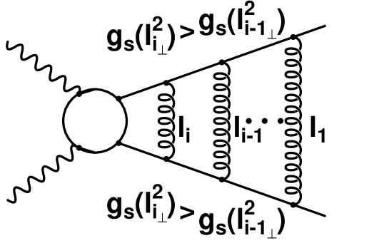
Figure 1: A schematic Feynman diagram leading to the Sudakov double logarithms in the process $\gamma\gamma(J_{z}=0)\longrightarrow q\overline{q}$ with $i$ gluon insertions. The blob denotes a hard momentum flowing through the omitted propagator in the DL-phase space. Crossed diagrams lead to a different ordering of the Sudakov variables with all resulting $C_{A}$ terms canceling the DL-contributions from three gluon insertions [18]. The scale of the coupling $\alpha_{s}=\frac{g_{s}^{2}}{4\pi}$ is indicated at the vertices and explicitly taken into account in this work.

In the derivation of the leading logarithmic corrections in Ref. [18] the familiar Sudakov technique [21] of decomposing loop momenta into components along external momenta, denoted by $\{\alpha,\beta\}$, and those perpendicular to them, denoted by $l_{\perp}$ was used. For massless fermions, the effective scale for Sudakov double logarithms for the coupling at each loop is $\alpha_{s}({\bf l^{2}_{\perp}})$, as was shown e.g. in Refs. [22, 23, 24] by direct comparison with explicit higher-order calculations. For massive fermions the effective scale is also given by ${\bf l^{2}_{\perp}}\equiv-l^{2}_{\perp}>0$ as the dominant double logarithmic phase space is given by $\frac{m^{2}}{s}\ll\frac{{\bf l^{2}_{\perp}}}{s}\ll 1$ [18] (on a formal DL level, setting $m=\lambda$ yields the massless Sudakov form factor). We use

$$\alpha_{s}({\bf l^{2}_{\perp}})=\frac{\alpha_{s}(m^{2})}{1+\beta_{0}\frac{\alpha_{s}(m^{2})}{\pi}\log\frac{{\bf l^{2}_{\perp}}}{m^{2}}+\beta_{1}\left(\frac{\alpha_{s}(m^{2})}{\pi}\right)^{2}\log\frac{{\bf l^{2}_{\perp}}}{m^{2}}}\equiv\frac{\alpha_{s}(m^{2})}{1+c\;\log\frac{{\bf l^{2}_{\perp}}}{m^{2}}}$$ (4)

where $\beta_{0}=\frac{11}{12}C_{A}-\frac{4}{12}T_{F}n_{F}$, $\beta_{1}=\frac{17}{24}C_{A}^{2}-\frac{5}{12}C_{A}T_{F}n_{F}-\frac{1}{4}C_{F}T_{F}n_{F}$ and for QCD we have $C_{A}=3$, $C_{F}=\frac{4}{3}$ and $T_{F}=\frac{1}{2}$ as usual. Up to two-loops the massless $\beta$-function is independent of the chosen renormalization scheme and is gauge invariant in minimally subtracted schemes to all orders [25]. These features also hold for the renormalization group improved form factors below.

For the massive Sudakov form factor we use the on-shell condition ${\bf l^{2}_{1_{\perp}}}=s\alpha_{1}\beta_{1}$, even though the running coupling will now depend on two integration variables. Since in this work we are only able to include the hard one-gluon matrix elements (the exact NNLO corrections are presently unknown), the higher-order terms will inevitably be energy cut ($l_{c}$) dependent. However our two-jet definition (see below) automatically restricts the higher-order hard gluon radiation phase space such that it is reasonable to neglect more than one gluon emission. The complete result for the renormalization group improved massive Sudakov form factor is then given by [20]:

$$\widetilde{{\cal F}}^{RG}_{S_{R}}+2\widetilde{{\cal F}}^{RG}_{S_{V}} = \frac{\alpha_{s}(m^{2})C_{F}}{\pi}\left\{\frac{1}{c}\int_{\frac{2l_{c}m^{2}}{(s+m^{2})\sqrt{s}}}^{\frac{2l_{c}\sqrt{s}}{s+m^{2}}}\frac{d\beta_{1}}{\beta_{1}}\log\frac{1+c\;\log\left(\left(\frac{2l_{c}}{\sqrt{s}}-\beta_{1}\right)\beta_{1}\frac{s}{m^{2}}\right)}{\left(1+c\;\log\frac{s\beta_{1}}{m^{2}}\right)}\right.$$ (5)

$$-\frac{1}{c}\log\frac{s}{m^{2}}\log\frac{\alpha_{s}(2l_{c}\sqrt{s})}{\alpha_{s}(s)}-\frac{1}{c}\log\frac{2l_{c}}{\sqrt{s}}\log\frac{\alpha_{s}(2l_{c}\sqrt{s})}{\alpha_{s}\left(\frac{2l_{c}m^{2}}{\sqrt{s}}\right)}$$

$$\left.-\frac{1}{c^{2}}\log\frac{\alpha_{s}(m^{2})\alpha_{s}(2l_{c}\sqrt{s})}{\alpha_{s}(s)\alpha_{s}\left(\frac{2l_{c}m^{2}}{\sqrt{s}}\right)}+\frac{1}{2}\log\frac{s}{m^{2}}+\log\frac{s}{4l_{c}^{2}}-1+\frac{\pi^{2}}{3}\right\}\;,$$

assuming only $\frac{m^{2}}{s}\ll 1$. Expanding in $\alpha_{s}(m^{2})$ gives the DL-Sudakov form factor in Eq. 3 together with subleading terms proportional to $\beta_{0}$ and subsubleading terms proportional to $\beta_{1}$. We emphasize that the two-loop running coupling is included in Eq. 5 to all orders and that all collinear divergences are avoided by keeping all non-homogeneous fermion mass terms. In Ref. [20] it was shown that Eq. 5 exponentiates in analogy to the soft exponential term in Eq. 3. The reason for adopting the above soft gluon energy regulator rather than the more conventional $y_{cut}$ invariant mass prescription (see Refs. [12, 15, 16] for instance) is connected with the straightforward DL-phase space of the massive Sudakov form factor. The latter is thus convenient for the inclusion of the renormalization group effects as outlined above. More details are given in Ref. [20].

Figure 2: The schematic Feynman diagrams leading to the non-Sudakov double logarithms in the process $\gamma\gamma(J_{z}=0)\longrightarrow q\overline{q}$ with $i+1$ gluon insertions. The blobs denote a hard momentum flowing through the omitted propagator in the DL phase space. Crossed diagrams lead to a different ordering of the Sudakov variables and are correctly accounted for by a factor of $(i+1)!$ at each order. The scale of the coupling $\alpha_{s}=\frac{g_{s}^{2}}{4\pi}$ is indicated at the vertices and included explicitly in the calculation. The topology on the left-hand diagram is Abelian like, and the one on the right is non-Abelian beyond one-loop.

We next turn to the virtual non-Sudakov DL corrections and investigate the RG effects for these contributions. Here we use the scale ${\bf l_{\perp}^{2}}$ directly as the graphs in Fig. 2 are on a DL level identical to the Sudakov topology up to the last integration over the (regulating) fermion line. This last integration, however, does not renormalize the coupling. For the non-Sudakov topologies depicted in Fig. 2 we find, after an order-by-order integration over the appropriate running coupling for the complete virtual renormalization group improved non-Sudakov form factor:

$$\widetilde{{\cal F}}_{h}^{RG} = \sum^{\infty}_{i=0}\int^{s}_{m^{2}}\frac{d{\bf l^{2}_{\perp}}}{{\bf l^{2}_{\perp}}}\left(\frac{C_{F}}{2\pi}\right)^{i+1}\left(\frac{\alpha_{s}(m^{2})}{c}\right)^{i}\frac{\alpha_{s}({\bf l^{2}_{\perp}})}{(i+1)!}\log^{i+1}\frac{{\bf l^{2}_{\perp}}}{s}\log^{i}\frac{\alpha_{s}(m^{2})}{\alpha_{s}({\bf l^{2}_{\perp}})}+$$ (6)

$$2\sum^{\infty}_{i=0}\int^{s}_{m^{2}}\frac{d{\bf l^{2}_{\perp}}}{{\bf l^{2}_{\perp}}}\frac{C_{F}C_{A}^{i}}{2^{2i+1}\pi^{i+1}}\left(\frac{\alpha_{s}(m^{2})}{c}\right)^{i}\frac{\alpha_{s}({\bf l^{2}_{\perp}})}{(i+1)!}\log^{i+1}\frac{{\bf l^{2}_{\perp}}}{s}\log^{i}\frac{\alpha_{s}(m^{2})}{\alpha_{s}({\bf l^{2}_{\perp}})}\;,$$

and thus for the RG-improved virtual plus soft real cross section we have

$$\frac{\sigma^{DL}_{RG}}{\sigma_{\rm Born}}=\left\{1+\widetilde{{\cal F}}_{h}^{RG}\right\}^{2}\exp\left(\widetilde{{\cal F}}^{RG}_{S_{R}}+2\widetilde{{\cal F}}^{RG}_{S_{V}}\right)$$ (7)

Figure 3: The effect of the renormalization group improved form factor (circles) of Eq. 7 in comparison to using the DL form factors of Eq. 3 with the indicated values of the strong coupling. The upper plot corresponds to $l_{c}=0.1\sqrt{s}$ and the lower one to $l_{c}=0.05\sqrt{s}$. The effect is displayed for the bottom quark with $m_{b}=4.5$ GeV.

where the RG-improved massive Sudakov form factor is given in Eq. 5. The effect of the renormalization group improved virtual plus soft real bremsstrahlung cross section is depicted in Fig. 3. The RG-improved cross section obtained using Eq. 7 lies between the theoretically allowed upper and lower limits given by the double logarithmic form factor of Eq. 3 with $\alpha_{s}$ evaluated at the bottom mass and the Higgs mass scale. For a lower value of the energy cutoff $l_{c}$ the background is more suppressed but the higher order (uncanceled) $l_{c}$-dependence is stronger. This latter technical problem can be reduced by identifying $l_{c}$ with the physical energy cutoff of the detector efficiencies. This will be discussed in section 4.

3 Radiative Corrections to $\gamma\gamma\longrightarrow H\longrightarrow q\overline{q}$

An intermediate mass Higgs boson has a very narrow total decay width. It is therefore appropriate to compare the total number of Higgs signal events with the number of (continuum) background events integrated over a narrow energy window around the Higgs mass. The size of this window depends on the level of monochromaticity that can be achieved for the polarized photon beams.

In general, the number of events for the (signal) process $S$ is given by

$$N_{S}=\int\frac{dL}{dw}\sigma_{S}(w)dw$$ (8)

where $w$ denotes the center of mass energy. For $S\equiv\gamma\gamma\longrightarrow H\longrightarrow b\overline{b}$ we have the following Breit-Wigner cross section, e.g. Refs. [26, 27]:

$$\sigma_{S}(w)=\frac{16\pi\Gamma(H\longrightarrow\gamma\gamma)\Gamma(H\longrightarrow b\overline{b})}{(w^{2}-m^{2}_{H})^{2}+\Gamma_{H}^{2}m^{2}_{H}}(\hbar c)^{2}$$ (9)

where the conversion factor $(\hbar c)^{2}=3.8937966\times 10^{11}$ fb GeV². In the narrow width approximation we then find for the expected number of events

$$N_{S}=\left.\frac{dL_{\gamma\gamma}}{dw}\right|_{m_{H}}\frac{8\pi^{2}\Gamma(H\longrightarrow\gamma\gamma)BR(H\longrightarrow b\overline{b})}{m^{2}_{H}}(\hbar c)^{2}$$ (10)

To quantify this, we take the design parameters of the proposed TESLA linear collider [28, 29], which correspond to an integrated peak $\gamma\gamma$-luminosity of 15 fb^-1 for the low energy running of the Compton collider. The polarizations of the incident electron beams and the laser photons are chosen such that the product of the helicities $\lambda_{e}\lambda_{\gamma}=-1$ . This ensures high monochromaticity and polarization of the photon beams [5, 6, 28, 29, 30]. Within this scenario a typical resolution of the Higgs mass is about 10 GeV, so that for comparison with the background process $BG\equiv\gamma\gamma\longrightarrow q\overline{q}$ one can use [26, 27]:

$$\frac{L_{\gamma\gamma}}{10\;{\rm GeV}}=\left.\frac{dL_{\gamma\gamma}}{dw}\right|_{m_{H}}$$ (11)

with $\left.\frac{dL_{\gamma\gamma}}{dw}\right|_{m_{H}}=$0.5 fb^-1/GeV. The number of background events is then given by

$$N_{BG}=L_{\gamma\gamma}\sigma_{BG}\;.$$ (12)

In other words, the number of signal events is proportional to $N_{S}\sim\left.\frac{dL_{\gamma\gamma}}{dw}\right|_{m_{H}}$ while the number of continuum heavy quark production events is proportional to $N_{BG}\sim L_{\gamma\gamma}$. In principle it is possible to use the exact Compton profile of the backscattered photons to obtain the full luminosity distributions. The number of expected events is then given as a convolution of the energy dependent luminosity and the cross sections. Our approach described above corresponds to an effective description of these convolutions, since these functions are not precisely known at present. Note that the functional forms currently used generally assume that only one scattering takes place for each photon, which may not be realistic. Once the exact luminosity functions are experimentally determined it is of course trivial to incorporate them into a Monte Carlo program containing the physics described in this paper.

Figure 4: The Standard Model process $\gamma\gamma\longrightarrow H\longrightarrow b\overline{b}$ is mediated by $W-$boson and $t$- and $b$-quark loops.

We next summarize the radiative corrections entering into the calculation of the expected number of Higgs events. For the quantity $\Gamma(H\longrightarrow\gamma\gamma)$ there are three main Standard Model contributions, depicted in Fig. 4: the $W^{\pm}$ and $t$- and $b$-quark loops. We include these at the one-loop level, since the radiative corrections are significant only for the $b$-quark [7]. The branching ratio $BR(H\longrightarrow b\overline{b})$ is treated in the following way. The first component consists of the partial $\Gamma(H\longrightarrow b\overline{b})$ width. Obviously we must use the same two-jet criterion for the signal as for the background. For our purposes a cone-type algorithm is most suitable, and so we use the Sterman-Weinberg two-jet definition [31] depicted in Fig. 5. Note that the signal cross section is corrected by the same resummed renormalization group improved form factor given in Eq. 5, since this factor does not depend on the spin of the particle coupling to the final state quark anti-quark pair.

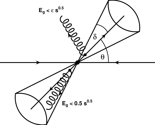
Figure 5: The parameters of the Sterman-Weinberg two-jet definition used in this work. Inside an angular cone of size $\delta$ arbitrary hard gluon bremsstrahlung is included. Radiation outside this cone is only permitted if the gluon energy is below a certain fraction ($\epsilon$) of the incident center of mass energy. The thrust angle is denoted by $\theta$.

In addition we use the exact one-loop corrections from Ref. [32]. These revealed that the largest radiative corrections are well described by using the running quark mass evaluated at the Higgs mass scale. We therefore resum the leading running mass terms to all orders. For the real bremsstrahlung corrections we use our own $H\longrightarrow q\bar{q}g$ matrix elements. An important check is obtained by integrating over all phase space and reproducing the analytical results of Ref. [32].

The second quantity entering the branching ratio is the total Higgs width $\Gamma_{H}$. Here we use the known results summarized in Ref. [7], and include the partial Higgs to $b\overline{b}$, $c\overline{c}$, $\tau^{+}\tau^{-}$, $WW^{*}$, $ZZ^{*}$ and $gg$ decay widths with all relevant radiative corrections.

4 Numerical Results

In Ref. [20] numerical predictions were given for an (infra-red safe) two-jet $b\bar{b}$ cross section in $\gamma\gamma$ collisions in the energy range $\sqrt{s}=100-160$ GeV. A modified Sterman-Weinberg cone definition, imposed on the final state partons was employed. Thus, at leading order (i.e. $\gamma\gamma\to b\overline{b}$) all events obviously satisfy the two–$b$–jet requirement. This defines our ‘leading order’ (LO) cross section. At next–to–leading order (NLO) we can have virtual or real gluon emission. For the latter, an event is defined as two–$b$–jet like if the emitted gluon

either $$\mbox{I.\quad~{}has energy less than $\epsilon\sqrt{s}$, with $\epsilon\ll 1$},$$

or $$\mbox{II.\quad is within an angle $2\delta$ of the $b$ or $\overline{b}$, again with $\delta\ll 1$}.$$

We further subdivided region I according to whether the gluon energy is greater or less than the infrared cutoff $l_{c}$ ($<\epsilon$). Adding the virtual gluon corrections to this latter (soft) contribution, to give $\sigma_{\rm SV}$, and calling the remaining hard gluon contribution $\sigma_{\rm H}$, we have

$$\sigma_{\rm 2j}=\sigma_{\rm SV}(l_{c})+\sigma_{\rm H}(l_{c},\epsilon,\delta)\;.$$ (13)

In Ref. [19] each part of this cross section was evaluated exactly to ${\cal O}(\alpha_{s})$ and in addition the resummed non-Sudakov form factor was included in $\sigma_{\rm SV}$. This was necessary to yield a positive cross section.

We use the RG-improved expressions for the resummed form factors. Thus

$$\sigma_{\rm SV}\longrightarrow\sigma^{DL}_{RG}+\tilde{\sigma}_{\rm SV}\;,$$ (14)

where $\sigma^{DL}_{RG}$ is given in Eq. 7 and $\tilde{\sigma}_{\rm SV}$ is the exact one-loop result minus the one-loop leading-logarithm pieces which are resummed in $\sigma^{DL}_{RG}$, i.e.

$$\tilde{\sigma}_{\rm SV} = \sigma_{\rm SV,NLO}-\sigma_{\rm LO}\left[-6{\cal F}+\frac{\alpha_{s}C_{F}}{\pi}\left(\log\frac{s}{m_{q}^{2}}\left(\frac{1}{2}-\log\frac{s}{4l_{c}^{2}}\right)+\log\frac{s}{4l_{c}^{2}}-1+\frac{\pi^{2}}{3}\right)\right]\;.$$

By adding the second (Sudakov) piece in the square brackets we remove (at least up to terms ${\cal O}(l_{c}^{2}/s)\ll 1$) the dependence on the gluon energy cutoff $l_{c}$. Note also that the complete expression for the two-jet cross section (with the remaining $l_{c}$ dependence displayed)

$$\sigma_{\rm 2j}=\sigma^{DL}_{RG}(l_{c})+\tilde{\sigma}_{\rm SV}+\sigma_{\rm H}(l_{c},\epsilon,\delta)\;.$$ (16)

contains a mixture of exact ${\cal O}(\alpha_{s})$ and resummed pieces. For the former, we use $m_{q}^{2}$ as the scale for $\alpha_{s}$. The resummed contributions are based on the scale choice ${\bf l^{2}_{\perp}}$ in the loops, as already discussed.

Before computing and combining the various components of the two-jet cross section in Eq. 16 we must address the issue of the dependence on the unphysical infra-red parameter $l_{c}$. If we were to expand out the resummed RG-improved form factor $\sigma^{DL}_{RG}(l_{c})$ in powers of $\alpha_{s}(m_{q}^{2})$, and retain only the ${\cal O}(\alpha_{S})$ term, we would find that the $l_{c}$ dependence exactly canceled that of $\sigma_{\rm H}(l_{c},\epsilon,\delta)$. However in the full resummed expression, there is nothing to cancel the explicit $l_{c}$ dependence at higher-orders. The canceling terms would come from the as yet unknown higher-order contributions to $\sigma_{\rm H}$. Faced with this dilemma, we have several choices. We could, as in [19], neglect the higher-order terms in the Sudakov form factor altogether, and include only the non-Sudakov form factor which is of course independent of $l_{c}$. Furthermore, as shown in [19] with the choice $\epsilon={\cal O}(0.1)$, the combined contribution of virtual gluons and real gluons with $E_{g}<\epsilon\sqrt{s}$ to $\sigma_{\rm 2j}$ was dominated by the non-Sudakov ‘$6{\cal F}$’ part. This suggests that the most reasonable procedure for the resummed cross section is to take $l_{c}\sim\epsilon\sqrt{s}$ and to vary $\epsilon$. We stress that this is an approximation, since it corresponds to making an assumption about the contribution of real multi-gluon emission with energies $<{\cal O}(\epsilon\sqrt{s})$.

As our ‘best guess’ RG-improved, resummed two-jet cross section, therefore, we have

$$\sigma_{\rm 2j}=\sigma^{DL}_{RG}(\epsilon\sqrt{s})+\tilde{\sigma}_{\rm SV}+\sigma_{\rm H}(\epsilon\sqrt{s},\epsilon,\delta)\;.$$ (17)

At this point it is appropriate to comment on detector and accelerator related issues which were adopted in our analyses [33]. Since we are not using a full detector simulation we employ effective performance parameters which should be achievable at a future linear collider. We will display results for realistic scenarios for both currently accepted and more optimistic cases. In particular the double b-tagging efficiency will be assumed to be $70\%$ throughout and the main input parameters concern the probability of counting a $c\overline{c}$-pair as $b\overline{b}$ and the ratio of the photon-pairs in a $J_{z}=0$ to $J_{z}=\pm 2$ state. We emphasize again that these dependences are in real machine environment given by functional forms which can easily be determined through test runs at a later stage. For our purposes here the effective description is sufficient.

The results discussed in the next section contain all radiative corrections summarized above. The goal is to optimize the jet-parameters of the Sterman-Weinberg two-jet definition in order to maximize the statistical significance of the intermediate mass Higgs-boson signal.

4.1 Discussion of the MC Results

We begin with a few generic remarks concerning the uncertainties in our predictions. The signal process $\gamma\gamma\longrightarrow H\longrightarrow b\overline{b}$ is well understood and NNL calculations are available. The theoretical error is thus negligible [7].

There are two contributions to the background process $\gamma\gamma\longrightarrow q\overline{q}$ which we neglect in this paper. Firstly, the so-called resolved photon contribution [34] was found to be a small effect, e.g. [15, 16], especially since we want to reconstruct the Higgs mass from the final two-jet measurements and impose angular cuts in the forward region. In addition the good charm suppression also helps to suppress the resolved photon effects as they give the largest contribution. The second contribution we do not consider here results from the final state configuration where a soft quark is propagating down the beam pipe and the gluon and remaining quark form two hard back-to back-jets [12]. We neglect this contribution here due to the expected excellent double b-tagging efficiency and the strong restrictions on the allowed acollinearity discussed below .

For the continuum heavy quark production cross section an exact NLO calculation exists [15] but large radiative corrections in the $J_{z}=0$ channel require the resummation of large non-Sudakov DL’s as expounded on above. Assuming that the largest part of the NLO and higher subleading logarithms is contained in the renormalization of the strong coupling parameter $\alpha_{s}$, the virtual corrections seem to be well under control. The largest uncertainty we thus expect to be contained in the missing hard ${\cal O}\left(\alpha_{s}^{2}\right)$ bremsstrahlung corrections for which no $\frac{m_{q}^{2}}{s}$ suppression-factor exists. Theoretically, these can be controlled by limiting the available phase-space through a narrow two-jet definition. On the other hand this means that we would also lose (signal) events which is clearly undesirable. In light of these two effects we think it prudent to find a balancing middle ground for our MC-results. More details are given below.

A second source of uncertainty is contained in the higher order $l_{c}$-dependence as mentioned above. Our strategy of identifying $\epsilon\sqrt{s}=l_{c}$ is reasonable as long as the neglected ${\cal O}\left(\epsilon^{2}\right)$ terms (which have no Born cross section suppression) are negligible and can be identified with the physical detector energy cuts. In this paper we will thus study two different values for the energy cut: $\epsilon=0.1$ and $0.05$. The value of $\epsilon$ is related to the allowed acollinearity of the two jet alignments corresponding to acollinearities of $11.5^{o}$ and $5.73^{o}$. We emphasize that the requirement of a small jet acollinearity substantially suppresses the $J_{z}=\pm 2$ background component and could play an important role in improving the photon collider energy resolution [28, 29] as well as in the suppression of the background due to the resolved processes. Below we display results assuming in each case a (realistic) ratio of $J_{0}/J_{2}=20$ in parallel with the (optimistic) ratio of $J_{0}/J_{2}=50$.

We start with Fig. 6 assuming a (quite realistic) probability of counting a $c\bar{c}$- as a $b\bar{b}$-pair of $3\%$ and the Sterman-Weinberg parameters $\epsilon=0.1$ and $\delta=20^{o}$. The figure shows signal and BG events separately for two values of the thrust angle $\theta$ cut, $|\cos\theta|<0.7$ and $|\cos\theta|<0.5$. In both scenarios it can be seen that the largest component to the BG events for $J_{0}/J_{2}=20$ originates from the $J_{z}=\pm 2$ $c$-quark contribution. The second largest corrections stem from the $b$-quark for both $J_{z}=0$ and $J_{z}=\pm 2$ while the $J_{z}=0$ $c$-quark contribution is small.

The smaller thrust-cut two-jet definition eliminates more of the background events in relative terms. However, it also reduces the total number of events. Fig. 7 demonstrates that the $|\cos\theta|<0.5$ scenario yields roughly a 50 % higher ratio of signal to BG events. The inverse statistical significance of the Higgs-boson process, defined as $\sqrt{N_{tot}}/N_{S}$, however, is somewhat higher for the $|\cos\theta|<0.7$ choice as is demonstrated in Fig. 8. The difference between the realistic $J_{0}/J_{2}=20$ and optimistic $J_{0}/J_{2}=50$ photon-polarization cases is small. For the one-year running analysis of an intermediate mass Higgs with $m_{H}<140$GeV the inverse statistical significance is below 3%, which can be viewed as the minimal statistical expectation.

It seems now possible to assume an even better detector performance. The improvement comes from assuming a better single point resolution, thinner detector modules and moving the vertex detectors closer to the beam-line [33]. Thus we can assume a (still realistic) 1% probability of counting a $c\bar{c}$- as a $b\bar{b}$-pair. Figs. 9, 10 and 11 display the same observables for otherwise identical two-jet definitions and machine-parameters. The charm-contribution is visibly reduced and the number of signal to background events roughly 30% larger. The statistical accuracy for the Higgs signal, however, is only slightly enhanced.

With these results in hand we now keep $|\cos\theta|<0.7$ fixed and furthermore assume the $c\bar{c}$ misidentification rate of 1%. We vary the cone angle $\delta$ between narrow ($10^{o}$), medium ($20^{o}$) and large ($30^{o}$) cone sizes for both $\epsilon=0.1$ and $\epsilon=0.05$. The upper row of Fig. 12 demonstrates that for the former choice of the energy cutoff parameter we achieve the highest statistical accuracy for the large $\delta=30^{o}$ scenario of around 2%. We again emphasize, however, that in this case also the missing ${\cal O}\left(\alpha_{s}^{2}\right)$ bremsstrahlung corrections could become important.

The largest effect is obtained by effectively suppressing the background radiative events with the smaller energy cutoff of $\epsilon=0.05$ outside the cone (the inside is of course independent of $\epsilon$). Here the lower row of Fig. 12 demonstrates that the statistical accuracy of the Higgs boson with $m_{H}<140$ GeV can be below the 2% level after collecting one year of data. We should mention again that for this choice of $\epsilon$ we might have slightly enhanced the higher order (uncanceled) cutoff dependence. The dependence on the photon-photon polarization degree is visible but not crucial.

In summary, it seems very reasonable to expect that at the Compton collider option we can achieve a 2% statistical accuracy of an intermediate mass Higgs boson signal after collecting data over one year of running.

5 Conclusions

In this paper we have studied the Higgs signal and continuum background contributions to the process $\gamma\gamma\longrightarrow b\overline{b}$ at a high-energy Compton collider. We have used all relevant QCD radiative corrections to both the signal and BG production available in the literature. The Monte Carlo results using a variety of jet-parameter variations revealed that the intermediate mass Higgs signal can be expected to be studied with a statistical uncertainty between $3\%$ in a very realistic and $1.6\%$ in an optimistic scenario after one year of collecting data.

Together with the expected uncertainty of 1% from the $e^{+}e^{-}$ mode determination of BR$(H\longrightarrow b\bar{b})$, and assuming four years of collecting data, we conclude that statistically a measurement of the partial width $\Gamma(H\longrightarrow\gamma\gamma)$ below the 2% precision level should be possible. This level of accuracy could significantly enhance the kinematical reach of the MSSM parameter space in the large pseudoscalar mass limit and thus open up a window for physics beyond the Standard Model.

For the total Higgs width, the main uncertainty is given by the error in the branching ratio BR$(H\longrightarrow\gamma\gamma)$, which at present is estimated at the 15 % level [35]. For Higgs masses above 110 GeV, the total Higgs width could be determined more precisely through the Higgs-strahlung process [36, 37] and its decay into $WW^{*}$ [38]. This is only possible, however, if the supersymmetric lightest Higgs boson coupling to vector bosons is universal (i.e. the same for $hWW$ and $hZZ$) and provided the optimistic luminosity assumptions can be reached.

In summary, using conservative machine and detector design parameters, we conclude that the Compton collider option at a future linear collider can considerably extend our ability to discriminate between the SM and MSSM scenarios.

Acknowledgements
We would like to thank M. Battaglia, G. Jikia, R. Orava, M. Piccolo and especially V.I. Telnov for useful discussions. This work was supported in part by the EU Fourth Framework Programme ‘Training and Mobility of Researchers’, Network ‘Quantum Chromodynamics and the Deep Structure of Elementary Particles’, contract FMRX-CT98-0194 (DG 12 - MIHT).

Figure 6: The number of both signal and background events for jet parameters $\epsilon=0.1$ and $\delta=20^{o}$ and the indicated values of the thrust angle $\theta$. The upper row assumes a ratio of $J_{0}/J_{2}=20$ and the lower row of $50$. The background is composed of bottom and charm contributions assuming 70 % double b-tagging efficiency and a 3 % probability to count a $c\overline{c}$ pair as $b\overline{b}$. The dash-dotted line corresponds to $J_{z}=\pm 2$ for $m_{c}$, the full line to $J_{z}=0$ for $m_{b}$, the dotted line to $J_{z}=\pm 2$ for $m_{b}$ and the dashed line to $J_{z}=0$ for $m_{c}$. All lines are are normalized to add up to the total background and all radiative corrections discussed in the text are included.

Figure 7: The ratio of signal to background events based on the jet parameters of Fig. 6. The smaller phase space cut $|\cos\theta|<0.5$ gives a larger ratio as expected.

Figure 8: The statistical accuracy of the measurement based on a one year running with the parameters of Fig. 6. The larger thrust angle cut gives a slightly better statistical significance.

Figure 9: The number of both signal and background events for jet parameters $\epsilon=0.1$ and $\delta=20^{o}$ and the indicated values of the thrust angle $\theta$. The upper row assumes a ratio of $J_{0}/J_{2}=20$ and the lower row of $50$. The background is composed of bottom and charm contributions assuming 70 % double b-tagging efficiency and a 1 % probability to count a $c\overline{c}$ pair as $b\overline{b}$. The dash-dotted line corresponds to $J_{z}=\pm 2$ for $m_{c}$, the full line to $J_{z}=0$ for $m_{b}$, the dotted line to $J_{z}=\pm 2$ for $m_{b}$ and the dashed line to $J_{z}=0$ for $m_{c}$. All lines are are normalized to add up to the total background and all radiative corrections discussed in the text are included.

Figure 10: The ratio of signal to background events based on the jet parameters of Fig. 9. The smaller phase space cut $|\cos\theta|<0.5$ gives a larger ratio as expected.

Figure 11: The statistical accuracy of the measurement based on a one year running with the parameters of Fig. 9. The larger thrust angle cut gives a slightly better statistical significance.

Figure 12: The cone-angle dependence of the inverse statistical significance of the intermediate mass Higgs signal for the displayed values of thrust and energy cut parameters. Overall a 70% double b-tagging efficiency and a 1% charm misidentification rate are assumed. For larger values of $\delta$ the number of events is enlarged, however, the theoretical uncertainty increases. For smaller values of $\epsilon$ higher order cutoff dependent terms might become important.

References

- [1] J.H. Field, hep-ph/9810288, UGVA-DPNC-1998-10-180 and references therein.
- [2] H. Georgi, HUTP-78/A010. Apr 1978. 14pp. Published in Hadronic J.1:155, 1978.
- [3] S. Nie, M. Sher, WM-98-118. Nov 1998. 8pp. (3881890): hep-ph/9811234.
- [4] For a review see M. Sher,Phys.Rept.179:273-418, 1989.
- [5] I.F. Ginzburg et al., Nucl.Inst.Meth. 205, 1983, 47.
- [6] I.F. Ginzburg et al., Nucl.Inst.Meth. 219, 1984, 5.
- [7] M. Spira, hep-ph/9705337, Fortsch.Phys. 46:203-284, 1998.
- [8] A. Djouadi, V. Driesen, W. Hollik, J.I. Illana, hep-ph/9612362, Eur.Phys. J.C1:149-162, 1998.
- [9] K.A. Ispiryan, I.A. Nagorskaya, A.G. Oganesyan, V.A. Khoze, Sov.J.Nucl.Phys. 11, 1970, 712.
- [10] T. Barklow, SLAC-preprint, SLAC-PUB-5364, 1990.
- [11] J.F. Gunion, H.E. Haber, Phys.Rev. D48, 5109, 1993.
- [12] D.L. Borden, V.A. Khoze, J. Ohnemus, W.J. Stirling, Phys.Rev. D 50, 1994, 4499.
- [13] T. Kinoshita, J.Math.Phys. 3, 1962, 650.
- [14] T.D. Lee, M. Nauenberg, Phys.Rev. 133B, 1964, 1549.
- [15] G. Jikia, A. Tkabladze, Phys.Rev. D 54, 1996, 2030.
- [16] G. Jikia, A. Tkabladze, Nucl.Inst.Meth. A 355, 1995, 81.
- [17] V.S. Fadin, V.A. Khoze, A.D. Martin, Phys.Rev. D 56, 1997, 484.
- [18] M. Melles, W.J. Stirling, hep-ph/9807332, Phys.Rev. D59:094009, 1999.
- [19] M. Melles, W.J. Stirling, hep-ph/9810432, Eur.Phys.J.C9:101, 1999.
- [20] M. Melles, W.J. Stirling, hep-ph/9903507, to appear in Nucl.Phys. B.
- [21] V.V. Sudakov, Sov.Phys. JETP 3, 1956, 65.
- [22] S.J. Brodsky, SLAC-PUB-2447, 1979, unpublished.
- [23] Yu.L. Dokshitzer, D.I. Dyakonov, S.I. Troyan, Phys.Lett. 78B, 1978, 290; 79B, 1978, 269; Phys.Rep. 58, 1980, 269.
- [24] A.B. Carter, C.H. Llewellyn Smith, Nucl.Phys. B163, 1980, 93.
- [25] J. Collins, Renormalisation (Cambridge University Press, Cambridge, England, 1984).
- [26] D.L. Borden, D.A. Bauer, D.O. Caldwell, SLAC-PUB-5715, 1992, and UCSB-HEP-92-01, 1992.
- [27] D.L. Borden, D.A. Bauer, D.O. Caldwell, Phys.Rev. D48, 4018, 1993.
- [28] V.I. Telnov, hep-ex/9810019, KEK-PREPRINT-98-163; hep-ex/9802003, Int.J.Mod.Phys. A13: 2399, 1998.
- [29] V.I. Telnov, private communications.
- [30] V.P. Gavrilov, I.A. Nagorskaya, V.A. Khoze, Izvestiya AN Armenian SSR, Fizika 4, 1969, 137.
- [31] G. Sterman, S. Weinberg, Phys.Rev.Lett. 39, 1977, 1436.
- [32] E. Braaten, J.P. Leveille, Phys.Rev. D22, 1980, 715.
- [33] M. Battaglia, private communications.
- [34] M. Drees, M. Kramer, J. Zunft, P.M. Zerwas, Phys.Lett. B306:371-378, 1993.
- [35] J.C. Brient, The Higgs decay in 2 photons, ECFA/DESY working group.
- [36] J. Ellis, M.K. Gaillard, D.V. Nanopoulous, Nucl.Phys. B 106, 1976, 292.
- [37] B.L. Ioffe, V.A. Khoze, Leningrad preprint LENINGRAD-76-274, 1976, Sov.J.Part.Nucl. 9, 1978, 50.
- [38] G. Borisov, F. Richard, hep-ph/9905413, contribution to the international workshop on linear colliders, Sitges, Spain, April 28 - May 5, 1999.