Abstract

In this paper, radiative decays $\rho^{0}\rightarrow\pi^{+}\pi^{-}\gamma,\pi^{0}\pi^{0}\gamma$ ,$\phi\rightarrow K^{+}K^{-}\gamma,K^{0}\bar{K^{0}}\gamma$ are studied systematically in the U(3)${}_{L}\times$U(3)_R chiral theory of mesons. The theoretical differential spectrum with respect to photon energy and branch ratio for $\rho^{0}\rightarrow\pi^{+}\pi^{-}\gamma$ agree well with the experimental data. Differential spectrums and branch ratios for $\rho^{0}\rightarrow\pi^{0}\pi^{0}\gamma,\phi\rightarrow K^{+}K^{-}\gamma,\phi\rightarrow K^{0}\bar{K^{0}}\gamma$ are predicted. The process $\phi\to K^{0}\bar{K^{0}}\gamma$ is relevant to precision measurment of CP-violation parameters in the kaon systerm at a $\phi$-factory. We give a complete estimate of the branch ratio for this decay process by including scalar resonance $f_{0},a_{0}$ poles, nonresonant smooth amplitude and an abnormal parity process with $K^{*}$ pole which hasn’t been considered before. We conclude that processes with intermediate $K^{*}$ do not pose a potential background problem for $\phi\rightarrow K^{0}\bar{K}^{0}$ CP violation experiments.

13.40.Hq,12.39.Fe,12.40.Vv,14.40.Cs

I Introduction

Radiative decays $V\rightarrow P\bar{P}\gamma$(where V denotes vector mesons, P denotes pseudoscalar mesons) have attracted much interest in past decade[2–10]. The study of this kind of rare decays is important in hadron physics, both because it is intimately related to the QCD-inspired descriptions of the dynamics of mesons and because it has been urged by experiments. For example, the reaction $\phi\rightarrow K^{0}\bar{K^{0}}\gamma$ poses a possible backgroud problem of $\phi\rightarrow K^{0}\bar{K^{0}}$ at future $\phi$ factory. The latter process has been proposed as a way to study CP violation[1].

The purpose of our present paper is to systematically study the processes $\rho^{0}\rightarrow\pi^{+}\pi^{-}\gamma,\pi^{0}\pi^{0}\gamma$, $\phi\rightarrow K^{+}K^{-}\gamma,K^{0}\bar{K^{0}}\gamma$ in the framework of U(3)${}_{L}\times$U(3)_R chiral theory of mesons[12]. In this effective chiral model, all couplings among pseudoscalars, and its lowest resonances are fixed by introducing an universal coupling constant $g$. Thus, a unified description of mesons in the low energy is provided.

In fact, this effective model is an extended chiral quark model including $0^{-},1^{\pm}$ mesons. The chiral quark model, originated by Weinberg[13], and then developed by Manohar and Georgi[14], provides a QCD-inspired description on the simple constituent quark model. In the view of Manohar-Georgi model, between the chiral symmetry breaking scale($\Lambda_{\chi SB}\sim 1-2$GeV) and the confinement scale ($\Lambda_{QCD}\sim 0.1-0.3$GeV), the dynamical field freedom are constituent quarks(quasi-particle of quarks), gluons and Goldstone bosons associated with chiral symmetry spontaneously breaking. In this quasiparticle description, the effective gluon coupling is small and interactions between quarks and Goldstone bosons is important. The external gauge fields(e.g., photon field) can be introduced by localizing the global chiral symmetry. On the other hand, it is well known that in the electromagnetic interaction of mesons, the vector mesons play an essential role through VMD(Vector Meson Dominate)[18]. Therefore, it is quite nature to extend chiral quark model to include spin-1 meson resonances via VMD and via minimal coupling principle.

The U(3)${}_{L}\times$U(3)_R chiral theory of mesons has been studied extensively[12, 15, 16]. The basic inputs for it are the pseudoscalar decay constants $f_{P}$, vector meson mass $m_{V}$ and a universal coupling constant $g$. Predictions of this model are in good agreement with data[12, 15, 16]. In particular, in Ref.[17] it has been shown that the low energy limit of this theory is equivalent to the chiral perturbation theory, and the QCD constraints in Ref.[19] are satisfied by this model. Therefore, as an effective model of QCD, the U(3)${}_{L}\times$U(3)_R chiral theory of mesons is reliable.

The content of this paper is organized as follows. In Sec.2, we present a brief review of chiral quark model and the basic notations of the U(3)${}_{L}\times$U(3)_R chiral theory of mesons. In Sec.3 and Sec.4, the branch ratio for these decays are calculated respectively, and the gauge invariance of these decay amplitudes is checked explicitly. We give a summary of the results in Sec.5

II Chiral quark model and U(3)${}_{L}\times$U(3)_R chiral theory of mesons

The simplest parametrization of chiral quark model is[14]

$${\cal L}_{\chi}=\bar{\psi}(x)(i\gamma\cdot\partial-mu(x))\psi(x)$$ (1)

where

$$\psi = (u,d,s)^{T},$$

$$u(x) = {1\over 2}(1-\gamma_{5})U(x)+{1\over 2}(1+\gamma_{5})U^{{\dagger}},$$

$$U(x) = \exp(2i\lambda_{a}\Phi_{a}/f_{0}),$$

and $\lambda_{a}$ are Gell-Mann matrices of SU(3), $\Phi_{a}$ are fields of pseudoscalar meson octet and $f_{0}\simeq f_{\pi}=186MeV$, $m$ is a parameter related to the quark condensate.

This Lagrangian is invariant under global chiral symmetry transformation. The vector(${\cal V}_{\mu}$) and axial-vector(${\cal A}_{\mu}$) external field are introduced into ${\cal L}_{\chi}$ due to the requirment of local chiral symmetry, i.e., we can replace the derivative operator in Eq.(1) by covariant derivative operator with affine connection(or gauge potential) ${\cal V}_{\mu}+{\cal A}_{\mu}\gamma_{5}$ as follows:

$$\partial_{\mu}\rightarrow\tilde{\bigtriangledown}_{\mu}=\partial_{\mu}-i({\cal V}_{\mu}+{\cal A}_{\mu}\gamma_{5}).$$ (2)

Then we obtain a theory describing strong and elecro-weak interactions of mesons.

Spin-1 meson resonances can be included via VMD, i.e., via substitution of a new affine connection $(({\cal V}+v)_{\mu}+({\cal A}+a)_{\mu}\gamma_{5})$ for the former one ${\cal V}_{\mu}+{\cal A}_{\mu}\gamma_{5}$ in Eq.(2),

$$\tilde{\bigtriangledown}_{\mu}\rightarrow\tilde{\tilde{\bigtriangledown}}_{\mu}\equiv\partial_{\mu}-i(({\cal V}+v)_{\mu}+({\cal A}+a)_{\mu}\gamma_{5}),$$ (3)

with

$$a_{\mu}=\tau_{i}a^{i}_{\mu}+\lambda_{\alpha}K^{\alpha}_{1\mu}+(\frac{2}{3}+\frac{1}{\sqrt{3}}\lambda_{8})f_{\mu}+(\frac{1}{3}-\frac{1}{\sqrt{3}}\lambda_{8})f_{s\mu},$$ (4)

$$v_{\mu}=\tau_{i}\rho^{i}_{\mu}+\lambda_{\alpha}K_{\mu}^{*\alpha}+(\frac{2}{3}+\frac{1}{\sqrt{3}}\lambda_{8})\omega_{\mu}+(\frac{1}{3}-\frac{1}{\sqrt{3}}\lambda_{8})\phi_{\mu},$$ (5)

where $i$=1, 2, 3 and $\alpha$=4, 5, 6, 7.

Now, the author of Ref.[12] came to this extention and proposed a Lagrangian,

$${\cal L} = \bar{\psi}(x)(i\gamma\cdot(\partial-i((e_{0}QA+v)+a\gamma_{5}))-mu(x))\psi(x)+{1\over 2}m_{v}^{2}(v_{\mu a}v^{\mu}_{a}+a_{\mu a}a^{\mu}_{a}),$$ (6)

where $A_{\mu}$ is photon field, $Q$ is the electric charge. The mass term of $v$ and $a$ is chiral gauge invariant because the $v$ and $a$ transform homogeneously under local $U(3)_{L}\times U(3)_{R}$ symmetry. Note that there are no kinetic terms in Eq.(5) for all meson fields, since they are treated as composited fields of quark fields instead of the fundamental fields. The kinetic terms for these fields will be generated via loop effects of quarks.

Following Ref. [12], the effective Lagrangian of mesons (indicated by ${\cal M}$) are obtained through integrating over the quark fields,

$${\rm exp}\{i\int d^{4}x{\cal L^{M}}\}=\int[d\psi][d\bar{\psi}]{\rm exp}\{i\int d^{4}x{\cal L}\}.$$ (7)

Using the dimensional regularization, and in the chiral limit, the effective Lagrangian ${\cal L}_{RE}$ (normal parity part) and ${\cal L}_{IM}$ (abnormal parity part) have been evaluated in Refs.[12]. The Lagrangian describing normal parity processes reads

$${\cal L}_{RE} = {F^{2}\over 16}TrD_{\mu}UD^{\mu}U^{\dagger}-{\frac{g^{2}}{16}}Tr(L_{\mu\nu}L^{\mu\nu}+R_{\mu\nu}R^{\mu\nu})$$ (11)

$$+i\frac{N_{C}}{2(4\pi)^{2}}Tr(D_{\mu}UD_{\nu}U^{\dagger}L_{\nu\mu}+D_{\mu}^{\dagger}UD_{\nu}UR_{\nu\mu})+\frac{N_{C}}{6(4\pi)^{2}}TrD_{\mu}D_{\nu}UD^{\mu}D^{\nu}U^{\dagger}$$

$$-\frac{N_{C}}{12(4\pi)^{2}}Tr(D_{\mu}UD^{\mu}U^{\dagger}D_{\nu}UD^{\nu}U^{\dagger}+D_{\mu}U^{\dagger}D^{\mu}UD_{\nu}U^{\dagger}D^{\nu}U-D_{\mu}UD^{\nu}U^{\dagger}D_{\mu}UD^{\nu}U^{\dagger})$$

$$+{1\over 8}m_{0}^{2}Tr(L_{\mu}L^{\mu}+R_{\mu}R^{\mu}),$$

where

$$L_{\mu} = v_{\mu}-a_{\mu}\;,\;\;\;R_{\mu}=v_{\mu}+a_{\mu}\;,$$ (12)

$$D_{\mu}U = \bigtriangledown_{\mu}U-iL_{\mu}U+iUR_{\mu},$$ (13)

$$D_{\mu}U^{\dagger} = \bigtriangledown_{\mu}U^{\dagger}-iR_{\mu}U^{\dagger}+iU^{\dagger}L_{\mu},$$ (14)

$$L_{\mu\nu} = \bigtriangledown_{\mu}L_{\nu}-\bigtriangledown_{\nu}L_{\mu}-i[L_{\mu},L_{\nu}]+e_{0}QF^{L}_{\mu\nu}\;,$$ (15)

$$R_{\mu\nu} = \bigtriangledown_{\mu}R_{\nu}-\bigtriangledown_{\nu}R_{\mu}-i[R_{\mu},R_{\nu}]+e_{0}QF^{R}_{\mu\nu}\;,$$ (16)

$$\bigtriangledown_{\mu}\Psi = \partial_{\mu}\Psi+[-ie_{0}QA_{\mu},\Psi]\;\;\;\;\;\Psi=U,U^{\dagger},L,R,\;$$ (17)

$$F^{L}_{\mu\nu} = F^{R}_{\mu\nu}=\partial_{\mu}A_{\nu}-\partial_{\nu}A_{\mu}\;.$$ (18)

Here an universal coupling constant $g$ has been introduced to absorb the logarithmic divergence due to the integral of quark loop.

In Lagrangian ( 11) the field $a_{\mu}(x)$ mixes with $\partial_{\mu}{\Phi(x)}$, which should be diagonalized conveniently via field redefinition,

$$L_{\mu}\rightarrow L_{\mu}+i\frac{c}{g}U\bigtriangledown_{\mu}U^{\dagger}\;,$$ (19)

$$R_{\mu}\rightarrow R_{\mu}+i\frac{c}{g}U^{\dagger}\bigtriangledown_{\mu}U\;.$$ (20)

Then the following equations are derived,

$$\frac{F^{2}}{f_{\pi}^{2}}(1-\frac{2c}{g})=1,\;\;\;c=\frac{f_{\pi}^{2}}{2gm_{\rho}^{2}},\;\;\;\mbox{for two-flavor}.$$ (21)

$$\frac{F^{2}}{f_{K}^{2}}(1-\frac{2c^{\prime}}{g})=1,\;\;\;c^{\prime}=\frac{f_{K}^{2}}{2gm_{K^{*}}^{2}},\;\;\;\mbox{for three-flavor}$$ (22)

It should be stressed that this field redefinition is different from the one in Ref.[12], $a_{\mu}\rightarrow a_{\mu}-\frac{c}{g}\partial_{\mu}\Phi$. Eq.( 19) keeps the chiral symmetry explicitly. It plays an important role when we check the electromagnetic gauge invariance of the decay amplitude in following sections. Eq.(7)-Eq.(11) provide the formalism employed in this paper and all the calculations are performed in the chiral limit.

III The decay $\rho^{0}\rightarrow\pi^{+}\pi^{-}\gamma,\pi^{0}\pi^{0}\gamma$

In this section, we will restrict our calculations to the two-flavor case. The needed vertices to evaluate these processes can be obtained from Sec.2. For the reaction $\rho^{0}\rightarrow\pi^{+}\pi^{-}\gamma$, the Feynman diagrams are shown in Fig.1, the involved vertices are:

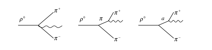
FIG. 1.: $\rho^{0}\rightarrow\pi^{+}\pi^{-}\gamma$

$${\cal L}_{\rho\pi\pi\gamma} = eA_{1}^{\rho}\rho_{\mu}A^{\mu}\pi^{i}\pi^{i}+eA_{2}^{\rho}\partial_{\mu}\rho_{\nu}F^{\mu\nu}\pi^{i}\pi^{i}{\;},$$ (23)

$${\cal L}_{\rho\pi\pi} = A_{1}^{\rho}\rho_{\mu}^{k}\pi^{i}\partial^{\mu}\pi^{j}\epsilon_{ijk}{\;},$$ (24)

$${\cal L}_{\rho{a}\pi} = \gamma\epsilon_{ijk}[B_{1}^{\rho}\partial_{\nu}\rho_{\mu}^{k}a^{\mu j}\partial^{\nu}\pi^{i}+B_{2}^{\rho}\partial_{\mu}\rho_{\nu}^{k}a^{\mu i}\partial^{\nu}\pi^{j}$$ (26)

$$+B_{3}^{\rho}\rho_{\mu}^{k}a_{\nu}^{i}\partial^{\mu\nu}\pi^{j}+B_{4}^{\rho}\partial^{2}\rho_{\mu}^{k}a^{\mu i}\pi^{j}],$$

$${\cal L}_{\gamma\pi\pi} = eA_{\mu}\pi^{i}\partial^{\mu}\pi^{j}\epsilon_{ijk}{\;},$$ (27)

$${\cal L}_{\gamma a\pi} = e\frac{\gamma f_{\pi}}{2g\pi^{2}F^{2}}F_{\mu\nu}a^{\mu i}\partial^{\nu}\pi^{j}\epsilon_{ijk}{\;},$$ (28)

where

$$A_{1}^{\rho} = \frac{2}{g}\{1+\frac{m^{2}_{\rho}}{2\pi^{2}f^{2}_{\pi}}[(1-\frac{2c}{g})^{2}-4\pi^{2}c^{2})]\},\;\;\;A_{2}^{\rho}=\frac{c-g}{g^{2}\pi^{2}F^{2}},$$ (29)

$$B_{1}^{\rho} = -\frac{f_{\pi}}{g^{2}\pi^{2}F^{2}}+\frac{8c}{gf_{\pi}\gamma^{2}},\;\;\;\;\;\;\;B_{2}^{\rho}=\frac{4c}{gf_{\pi}}+\frac{3f_{\pi}}{g^{2}\pi^{2}F^{2}},$$ (30)

$$B_{3}^{\rho} = \frac{4c}{gf_{\pi}}+\frac{2f_{\pi}}{g^{2}\pi^{2}F^{2}},\;\;\;\;\;\;\;\;\;B_{4}^{\rho}=\frac{1}{g^{2}\pi^{2}f_{\pi}},$$ (31)

$$\gamma = (1-\frac{1}{2g^{2}\pi^{2}})^{-\frac{1}{2}}.$$ (32)

The decay amplitude of this process is:

$${\cal M}_{\rho^{0}\rightarrow\pi^{+}\pi^{-}\gamma} = <\pi^{+}\pi^{-}\gamma|T\;\exp(i\int d^{4}x({\cal L}_{\rho\pi\pi\gamma}(x)+{\cal L}_{\rho\pi\pi}(x)+{\cal L}_{\rho{a}\pi}(x)+{\cal L}_{\gamma\pi\pi}(x)+{\cal L}_{\gamma a\pi}(x))|\rho>$$ (33)

$$= {\cal M}_{a}+{\cal M}_{b}+{\cal M}_{c}\;\;,$$ (34)

where

$${\cal M}_{a} = <\pi^{+}\pi^{-}\gamma|iT\;\int d^{4}x{\cal L}_{\rho\pi\pi\gamma}(x)|\rho^{0}>,$$ (35)

$${\cal M}_{b} = <\pi^{+}\pi^{-}\gamma|i^{2}T\;\int d^{4}x\int d^{4}y{\cal L}_{\rho\pi\pi}(x){\cal L}_{\gamma\pi\pi}(y)|\rho^{0}>,$$ (36)

$${\cal M}_{c} = <\pi^{+}\pi^{-}\gamma|i^{2}T\;\int d^{4}x\int d^{4}y{\cal L}_{\rho a\pi}(x){\cal L}_{\gamma a\pi}(y)|\rho^{0}>.$$ (37)

Since photon is on-shell in this process, we should check the gauge invariance of this amplitude. From Eq.(16) we see that the vertex of ${\cal L}_{\gamma a\pi}$ is already gauge invariant, therefore, we need to check only the sum of ${\cal M}_{a}$ and ${\cal M}_{b}$. One can derive from Eqs.(19–20) that

$${\cal M}_{a} = 2ie(A_{1}^{\rho}g_{\mu\nu}+A_{2}^{\rho}p\cdot qg_{\mu\nu}-A_{2}^{\rho}q_{\mu}p_{\nu})\varepsilon^{\mu}_{\vec{p}}e^{\nu}_{\vec{q}}\;,$$ (38)

$${\cal M}_{b} = 2ieA_{1}^{\rho}(\frac{k_{\mu}^{+}k_{\nu}^{-}}{q\cdot k^{-}}+\frac{k_{\mu}^{-}k_{\nu}^{+}}{q\cdot k^{+}})\varepsilon^{\mu}_{\vec{p}}e^{\nu}_{\vec{q}}\;,$$ (39)

where $p,k^{+},k^{-},q$ denote the momenta of $\rho^{0},\pi^{+},\pi^{-}$ and photon fields respectively, and $\varepsilon^{\mu}_{\vec{p}},e^{\nu}_{\vec{q}}$ are the polarization vectors for $\rho$ meson and photon field respectively. If we substitute $e^{\nu}_{\vec{q}}$ with $q^{\nu}$ in Eq.(22), we will obtain:

$$({\cal M}_{a}+{\cal M}_{b}){|}_{e^{\nu}_{\vec{q}}\rightarrow q^{\nu}}\propto(q_{\mu}+k^{+}_{\mu}+k^{-}_{\mu})\varepsilon^{\mu}_{\vec{p}}{\;}.$$ (40)

Using four-momentum conservation and the space-like condition of the wave function of vector field,

$$p=q+k^{+}+k^{-}{\;},$$ (41)

$$p\cdot\varepsilon_{\vec{p}}=0{\;}.$$ (42)

Eq.(22) vanishes, so the gauge invariance of this amplitude is kept.

Before we give the numerical results of the width and the branch ratio of this process, it is necessary to point out that there is no adjustable parameter in our calculation. The basic input $g$, as an universal coupling constant in this theory, can be fixed by a experiment, thus we can compare our theoretical results with experimental data and give predictions for processes which have not been measured in experiments. In this paper, we take $g=0.39$. Then we obtain,

$$\Gamma(\rho^{0}\rightarrow\pi^{+}\pi^{-}\gamma)=1.54\;\;\mbox{MeV}{\;},$$

$$B(\rho^{0}\rightarrow\pi^{+}\pi^{-}\gamma)=1.03\times 10^{-2}\;\;\;\;\;\;\;\mbox{for}\;\;E_{\gamma}>50\;\;\mbox{MeV}.$$

which compares favourably with the experimental data[20], $B^{exp}(\rho^{0}\rightarrow\pi^{+}\pi^{-}\gamma)=(0.99\pm 0.04\pm 0.15)10^{-2}$ for $E_{\gamma}>50$MeV, where $E_{\gamma}$ is the photon energy in the rest frame of $\rho^{0}$. The shape of differential spectrum with respect to photon energe is also given in the Fig. 6. One can see that the experimental result is in good agreement with our theoretical expectations.

The reaction $\rho^{0}\rightarrow\pi^{0}\pi^{0}\gamma$ involves only abnormal parity, the Feynman diagrams is shown in Fig.2. Following Ref.[12], by means of bosonization the quark propagator, we obtain

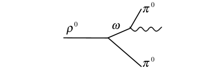
FIG. 2.: $\rho^{0}\rightarrow\pi^{0}\pi^{0}\gamma$

$${\cal L}_{\rho\omega\pi}=-\frac{3}{\pi^{2}g^{2}f_{\pi}}\varepsilon^{\mu\nu\alpha\beta}\partial_{\mu}\omega_{\nu}\rho_{\alpha}^{i}\partial_{\beta}\pi^{i}{\;},$$ (43)

$${\cal L}_{\gamma\omega\pi}=-e\frac{3}{2\pi^{2}gf_{\pi}}\varepsilon^{\mu\nu\alpha\beta}\partial_{\mu}\omega_{\nu}A_{\alpha}\partial_{\beta}\pi^{0}{\;}.$$ (44)

The vertex ${\cal L}_{\gamma\omega\pi}$ is obviously gauge invariant because of the totally antisymmetry tensor $\varepsilon^{\mu\nu\alpha\beta}$. The branch ratio is calculated to be

$$B(\rho^{0}\rightarrow\pi^{0}\pi^{0}\gamma)=1.02\times 10^{-5}{\;},$$ (45)

and the differential spectrum with respect to photon energy is shown in Fig.7 which will be tested in future experiments.

IV The decay $\phi\rightarrow K\bar{K}\gamma$

In order to calculate the $\phi$ decay, we need to extend our calculation to three-flavor case. First, we derive the vertices for the transition $\phi\rightarrow K^{+}K^{-}\gamma$, the Feynman digrams are shown in Fig.3, the vertices of this process have both normal parity part and abnormal parity part. The normal parity part is

$${\cal L}_{\phi K^{+}K^{-}\gamma} = eA_{1}^{\phi}\phi_{\mu}A^{\mu}K^{+}K^{-}{\;},$$ (46)

$${\cal L}_{\phi K^{+}K^{-}} = iA_{1}^{\phi}\phi_{\mu}K^{+}\partial^{\mu}K^{-}{\;},$$ (47)

$${\cal L}_{\gamma K^{+}K^{-}} = ieA_{\mu}K^{+}\partial^{\mu}K^{-}{\;},$$ (48)

$${\cal L}_{\phi K_{1}K} = \gamma[iB_{1}^{\phi}\partial_{\nu}\phi^{\mu}K_{1\mu}^{-}\partial^{\nu}K^{+}+iB_{2}^{\phi}\partial_{\mu}\phi^{\nu}K_{1\mu}^{-}\partial^{\nu}K^{+}+$$ (50)

$$iB_{3}^{\phi}\phi_{\mu}K_{1\nu}^{-}\partial^{\mu\nu}K^{+}+iB_{4}^{\phi}\partial^{2}\phi_{\mu}K_{1}^{\mu-}K^{+}]+h.c.{\;\;},$$

$${\cal L}_{\gamma K_{1}K} = ie\frac{\gamma f_{K}}{2g\pi^{2}F^{2}}F_{\mu\nu}K_{1}^{+\mu}\partial^{\nu}K^{-}+h.c.{\;\;},$$ (51)

where

$$A_{1}^{\phi} = -\frac{\sqrt{2}m_{\phi}^{2}}{f_{K}^{2}}[4c^{\prime}(1-{c^{\prime}\over g})+{1\over{g\pi^{2}}}(1-{2c^{\prime}\over g})^{2}],{\;\;\;\;}$$ (52)

$$B_{l}^{\phi} = \frac{\sqrt{2}}{2}{B_{l}^{\rho}(c\rightarrow c^{\prime},f_{\pi}\rightarrow f_{K})},{\;\;}l=1,2,3,4.$$ (53)

and the abnormal parity part is

$${\cal L}_{\phi K^{*}K^{\pm}} = -\frac{3\sqrt{2}}{2\pi^{2}g^{2}f_{K}}\varepsilon^{\mu\nu\alpha\beta}\partial_{\nu}\phi_{\alpha}K^{*+}_{\mu}\partial_{\beta}K^{-}+h.c.{\;\;},$$ (54)

$${\cal L}_{\gamma K^{*}K^{\pm}} = -\frac{e}{2\pi^{2}gf_{K}}\varepsilon^{\mu\nu\alpha\beta}\partial_{\nu}A_{\alpha}K^{*+}_{\mu}\partial_{\beta}K^{-}+h.c.{\;\;},$$ (55)

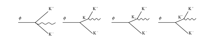
FIG. 3.: $\phi\rightarrow K^{+}K^{-}\gamma$

The gauge invariance can also be checked as in the $\rho$ decay. Using the same value of $g$, i.e., $g=0.39$, we give the differential spectrum in Fig.8 .

Now, we consider the transition $\phi\rightarrow K^{0}\bar{K^{0}}\gamma$. The photon in this reaction is very soft($E_{max}<25$Mev), so it is difficult to distinguish it from the genuine $\phi\rightarrow K^{0}\bar{K^{0}}$ events which has been proposed as a way to measure the small parameter in studying CP violation. The branch ratio of $\phi\rightarrow K^{0}\bar{K^{0}}\gamma(\stackrel{{\scriptstyle>}}{{\sim}}10^{-6})$ will limit the presion of this measurment. This quantity has been predicted by several authors[4-10]. In Refs.[4–8], the contribution of interchanging the scalar meson $S(a_{0},$or $f_{0}$) has been obtained via chain reaction $\phi\rightarrow S\gamma\rightarrow K^{0}\bar{K^{0}}\gamma$, in which the decay $\phi\rightarrow S\gamma$ is proceeds through the charged $K$ loop. The uncertainty of this approach is that the coupling constant $g_{SK\bar{K}}$ is not well know because of the lack of experiment data. In Ref.[9], the non-resonant contribution has been calculated using current algebra and low energy theorem. In Ref.[10], the authors did not introduce $a_{0},f_{0}$ explicitly, they calculated the final state intereaction of $KK$ system in a chiral unitary approach. This approach generates the $a_{0},f_{0}$ meson dynamically, the obtained amplitude after summing over an infinite series diagram also contain non-resonant contribution. All these calculations, however, did not contain the contribution of an abnormal parity process via interchanging $K^{*}$ which in principle must be added to the resonant poles and the nonresonant smooth amplitude, otherwise one may not assume scalar meson dominance a priori. In the present paper, we provide a complete calculation on the branch ratio for this decay by including the abnormal parity process with $K^{*}$ pole, scalar resonance $f_{0},a_{0}$ poles and non-resonant amplitude. The role of scalar resonance will be dealt with as in the former works[4–8,10]. The difference between their scheme and ours is that the needed vertices to calculate the loop diagram $\phi\to K^{+}K^{-}\gamma$ has been derived in Eqs.(28–30) as well as all the coupling constants has been fixed by the universal constant $g$, in other words, there is no adjustable parameter in our calculation. The complete intereaction of this process including normal and abnormal parity vertices is:

$${\cal L} = eA_{1}^{\phi}\phi_{\mu}A^{\mu}K^{+}K^{-}+iA_{1}^{\phi}\phi_{\mu}K^{+}\partial^{\mu}K^{-}+ieA_{\mu}K^{+}\partial^{\mu}K^{-}+{\cal L}_{\phi K^{*}K^{0}}+{\cal L}_{\gamma K^{*}K^{0}}$$ (56)

where

$${\cal L}_{\phi K^{*}K^{0}} = -\frac{3\sqrt{2}}{2\pi^{2}g^{2}f_{K}}\varepsilon^{\mu\nu\alpha\beta}\partial_{\nu}\phi_{\alpha}K^{*0}_{\mu}\partial_{\beta}\bar{K^{0}}+h.c.{\;\;},$$ (57)

$${\cal L}_{\gamma K^{*}K^{0}} = \frac{e}{\pi^{2}gf_{K}}\varepsilon^{\mu\nu\alpha\beta}\partial_{\nu}A_{\alpha}K^{*0}_{\mu}\partial_{\beta}\bar{K^{0}}+h.c.{\;\;},$$ (58)

described the abnormal parity process. Denoting the momenta of $K^{0},\bar{K^{0}}$ as $k_{1},k_{2}$ and defining $s_{1}=(k_{1}+q)^{2},s_{2}=(k_{2}+q)^{2}$, we derived the amplitude for this abnormal diagram(shown in Fig.4):

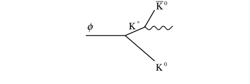
FIG. 4.: $\phi\to K^{0}\bar{K^{0}}\gamma$ through $K^{*}$.

$${\cal M}_{1} = <K^{0}\bar{K^{0}}\gamma|i^{2}T\;\int d^{4}x\int d^{4}y{\cal L}_{\phi K^{*}K^{0}}(x){\cal L}_{\gamma K^{*}\bar{K^{0}}}(y)|\phi>,$$ (59)

$$= ie\frac{3\sqrt{2}}{2\pi^{4}g^{3}f_{K}^{2}}(d_{0}g_{\mu\nu}+d_{1}k_{1\mu}k_{1\nu}+\tilde{d_{1}}k_{2\mu}k_{2\nu}+d_{2}k_{1\mu}k_{2\nu}+\tilde{d_{2}}k_{2\mu}k_{1\nu}){\;}\epsilon^{\mu}_{\vec{p}}e^{\nu}_{\vec{q}}$$ (60)

with

$$d_{0} = \frac{s_{1}}{4(s_{1}-m_{K^{*}}^{2})}(4k_{1}\cdot k_{2}+s_{1}-m_{\phi}^{2})+{\;}(k_{1}\leftrightarrow k_{2}),$$ (61)

$$d_{1} = {1\over 2}(\frac{s_{2}}{s_{2}-m_{K^{*}}^{2}}-\frac{m_{\phi}^{2}-s_{1}}{s_{1}-m_{K^{*}}^{2}}),{\;\;}\tilde{d_{1}}=d_{1}(k_{1}\leftrightarrow k_{2}),$$ (62)

$$d_{2} = \frac{s_{2}}{s_{2}-m_{K^{*}}^{2}}-\frac{k_{1}\cdot k_{2}}{s_{2}-m_{K^{*}}^{2}},{\;\;}\tilde{d_{2}}=d_{2}(k_{1}\leftrightarrow k_{2}).$$ (63)

In order to derive the contribution of scalar resonance $f_{0}$ and $a_{0}$, we need to calculate the one loop diagram though $K^{+}K^{-}$ and the final state intereactions of $K^{+}K^{-}$ to $K^{0}\bar{K^{0}}$ shown in Fig.5 .Similar to Ref.[10], we get the amplitude:

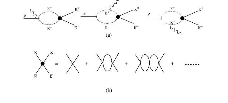
FIG. 5.: (a).$\phi\to K^{0}\bar{K^{0}}\gamma$ through charged $K$ loop. (b).$K^{+}K^{-}\to K^{0}\bar{K^{0}}$ amplitude, the intermediate loops contain $\pi\pi,K\bar{K},\pi^{0}\eta$.

$${\cal M}_{2} = \frac{eA_{1}^{\phi}}{2\pi^{2}im_{K}^{2}}I(a,b)[p\cdot qg_{\mu\nu}-p_{\nu}q_{\mu}]{\;}\epsilon^{\mu}_{\vec{p}}e^{\nu}_{\vec{q}}{\;}t_{s}$$ (64)

where $a={m_{\phi}^{2}}/{m_{K}^{2}},b={Q^{2}}/{m_{K}^{2}},Q^{2}=(k_{1}+k_{2})^{2}$,

$$I(a,b) = \frac{1}{2(a-b)}-\frac{2}{(a-b)^{2}}(f({1\over b})-f({1\over a}))+\frac{a}{(a-b)^{2}}(g({1\over b})-g({1\over a}))$$ (65)

with

$\displaystyle f(x)=\left\{\begin{array}[]{l}-\arcsin(\frac{1}{2\sqrt{x}})^{2}{\;\;\;}x>{1\over 4}\\ {1\over 4}[\ln(\frac{\eta_{+}}{\eta_{-}})-i\pi]^{2}{\;\;\;}x<{1\over 4}\end{array}\right.$

$\displaystyle g(x)=\left\{\begin{array}[]{l}(4x-1)^{1\over 2}\arcsin(\frac{1}{2\sqrt{x}})^{2}{\;\;\;}x>{1\over 4}\\ {1\over 2}(1-4x)^{1\over 2}[\ln(\frac{\eta_{+}}{\eta_{-}})-i\pi]^{2}{\;\;\;}x<{1\over 4}\end{array}\right.$

$$\eta_{\pm}={1\over{2x}}(1\pm\sqrt{1-4x})$$ (66)

the $t_{s}$(Eq.(9) in [10]) is the scattering amplitude of $K^{+}K^{-}$ to $K^{0}\bar{K^{0}}$, its diagrammatic meaning is shown in Fig.5(b), and its explicit expression can be obtained from Eq.(30) in Ref.[11] which is derived from Lippmann-Schwinger equation in the coupled channel approach. As declared in Ref.[10], this amplitude(Eq.(41)) also take into account nonresonant contribution.

The width and the branch ratio are given by:

$$\Gamma(\phi\rightarrow K^{0}\bar{K^{0}}\gamma) = \frac{\alpha}{192\pi^{2}m_{\phi}^{3}}\int ds_{1}dQ^{2}({\cal M}_{1}+{\cal M}_{2})^{2}$$ (67)

$$B(\phi\rightarrow K^{0}\bar{K^{0}}\gamma) = \Gamma(\phi\rightarrow K^{0}\bar{K^{0}}\gamma)/4.43$$ (68)

where $\alpha=e^{2}/4\pi=1/137$. In the following numerical evaluation, the constant $g$ take the same value 0.39 as in the previous. If we neglect the abnormal parity process, i.e. set ${\cal M}_{1}=0$, then we obtained $B(\phi\rightarrow K^{0}\bar{K^{0}}\gamma)_{scalar}=5.6\times 10^{-8}$, which is a little different with the value $5\times 10^{-8}$ quoted in Ref.[10]. On the other hand, if we neglect the contribution of scalar resonance, i.e. set ${\cal M}_{2}=0$, we obtained $B(\phi\rightarrow K^{0}\bar{K^{0}}\gamma)_{abnormal}=7.6\times 10^{-8}$. We see that the contribution of this abnormal parity process is the same important as the scalar resonance poles, so its contribution can not be neglected. After performing the integral of Eq.(44), we obtained:

$$B(\phi\rightarrow K^{0}\bar{K^{0}}\gamma) = 1.8\times 10^{-7}{\;}.$$ (69)

We see although the interference is constructive, it will not provide much significant background for precision test of CP-violation in $\phi\rightarrow K\bar{K}$. The differential spectrum with respect to photon energy for these three case(abnormal, scalar, interference) are given in Fig.9.

V Summary

To conclude, in this paper, we perform a systematic calculation of $\rho$ and $\phi$’s radiative decays in an extended chiral quark model, in which all coupling are fixed by the universal coupling constant $g$. The gauge invariance of these decay amplitudes has been checked. The theoretical differential spectrum with respect to photon energy and branch ratio of $\rho^{0}\rightarrow\pi^{+}\pi^{-}\gamma$ agree with the experimental data well. Predictions of differential spectrum and branch ratio for the processes $\rho^{0}\rightarrow\pi^{0}\pi^{0}\gamma,\phi\rightarrow K^{+}K^{-}\gamma,K^{0}\bar{K^{0}}\gamma$ have been derived. The branch ratio for $\phi\rightarrow K^{0}\bar{K^{0}}\gamma$ including the contribution of abnormal parity process with $K^{*}$ pole, scalar resonance $a_{0},f_{0}$ poles and nonresonant amplitude has been calculated to be about $10^{-7}$ and will not limit the precision measurment of the small CP-violation parameters at future $\phi$ factory.

ACKNOWLEDGMENTS

We would like to thank Dr. DaoNeng Gao for his helpful discussion. This work is partially supported by NSF of China through C. N. Yang and the Grant LWTZ-1298 of Chinese Academy of Science.

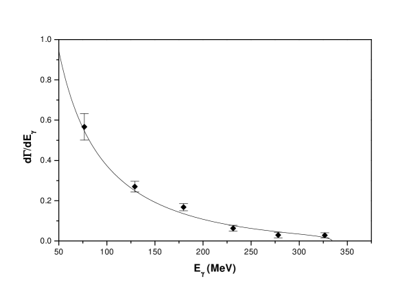
FIG. 6.: Photon spectrum,$d\Gamma/dE_{\gamma}$,for the process $\rho^{0}\to\pi^{+}\pi^{-}\gamma$. The experimental data taken from Ref.[20] are normalized to our results

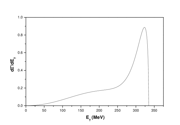
FIG. 7.: Photon spectrum, $d\Gamma/dE_{\gamma}$, for the process $\rho^{0}\rightarrow\pi^{0}\pi^{0}\gamma$.

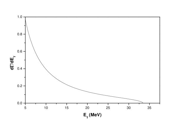
FIG. 8.: Photon spectrum, $d\Gamma/dE_{\gamma}$, for the process $\phi\rightarrow K^{+}K^{-}\gamma$. For $E_{\gamma}>5$MeV

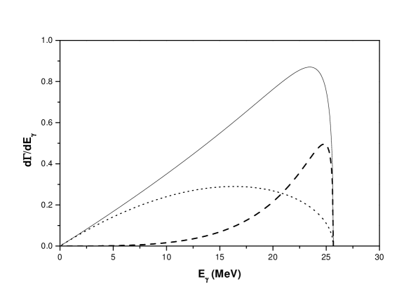
FIG. 9.: Photon spectrum, $d\Gamma/dE_{\gamma}$, for the process $\phi\rightarrow K^{0}\bar{K^{0}}\gamma$. Dot line: distribution only taking into account contribution of abnormal parity process with $K^{*}$ poles, dash line:distribution only taking into account the contribution of scalar resonance poles and nonresonant amplitude, solid line: the total distribution.