hep-ph/9907226 WUB 99-17 Phenomenology of $\eta\gamma$ and $\eta^{\prime}\gamma$ transition form factors
at large momentum transfer

Abstract

I discuss the progress in our theoretical understanding of the $\eta\gamma$ and $\eta^{\prime}\gamma$ transition form factors, including the recent data from CLEO and L3 at large momentum transfer, $Q^{2}$. The experimental data above $Q^{2}=1$ GeV² can be well described by the hard scattering approach if the distribution amplitudes for $\eta$ and $\eta^{\prime}$ mesons are taken close to the asymptotic one. Particular attention is paid to the interpretation of the data in terms of properly defined $\eta$-$\eta^{\prime}$ mixing parameters. I also comment on the use and misuse of interpolation formulas for $P\gamma$ and $P\gamma^{*}$ transition form factors. (Talk presented at conference Photon’99, Freiburg, May 1999)

1 Introduction

The hard exclusive production of pseudoscalar mesons $P=\pi^{0},\eta^{\phantom{.}},\eta^{\prime},\ldots$ in two-photon reactions provides an important process to test our understanding of QCD and to determine the properties of the pseudoscalar mesons. The calculation of the related transition form factor

$$\langle\gamma(q^{\prime},\varepsilon)|J_{\mu}^{\rm elm}|P(p)\rangle$$ (1)

$$= i\,e_{0}^{2}\,F_{P\gamma}(Q^{2})\,\epsilon_{\mu\alpha\beta\gamma}\,p^{\alpha}\,q^{\prime}{}^{\beta}\,\varepsilon^{\gamma}$$

at large virtualities of (at least) one of the two photons, $Q^{2}=(p-q^{\prime})^{2}\gg\Lambda_{\rm QCD}^{2}$, is based on the factorization of the amplitude into a short- and a long-distance part. The former can be calculated perturbatively by considering the elementary scattering of photons and quarks. In leading order this is a pure QED process, and thus uncertainties related to the value of $\alpha_{s}$ only enter on the level of QCD corrections. The long-distance part is expressed in terms of process-independent light-cone wave functions (LCWFs) of $q\bar{q}$- or eventually higher Fock states in the meson. The LCWFs parametrize the non-perturbative features related to, for instance, confinement. In the asymptotic limit, $Q^{2}\to\infty$, the behavior of the wave functions is known from the QCD evolution equation [1, 2]. For the $\pi\gamma$ transition form factor this leads to the famous prediction

$$\lim_{Q^{2}\to\infty}Q^{2}\,F_{\pi\gamma}(Q^{2}) = \sqrt{2}\,f_{\pi}\ .$$ (2)

The recent data from CLEO [3] at momentum transfer up to $15$ GeV² are still 10-15% below that limit, indicating that corrections to Eq. (2) have to be taken into account. In the standard hard-scattering approach (sHSA), see e.g. Ref. [4], one uses the collinear approximation (i.e. one neglects the transverse momenta of the partons) but includes radiative gluon corrections in fixed order perturbation theory. In the modified version of the hard-scattering approach (mHSA) also the effects connected to the transverse degrees of freedom are taken into account. In addition to the intrinsic transverse momenta a resummation of radiative gluon corrections accumulated in a Sudakov factor is included. The HSA gives a good description of the $\pi\gamma$ transition form factor at moderate values of $Q^{2}$ and indicates that the pion wave function is close to its asymptotic form already at small factorization scales, for details see e.g. Refs. [4, 5, 6] and references therein.

In this talk I will concentrate on the mHSA calculation of the $\eta\gamma$ and $\eta^{\prime}\gamma$ transition form factors [7]. Using the $\pi\gamma$ form factor as a case of reference, one obtains valuable information on the $\eta$ and $\eta^{\prime}$ properties. Especially the $\eta$-$\eta^{\prime}$ mixing parameters perfectly fit into the improved theoretical and phenomenological pattern which has been established recently in Refs. [8, 9].

2 MHSA calculation

Starting point of the calculation is a Fock-state expansion of the $\eta$ and $\eta^{\prime}$ mesons

$$|P\rangle = \sum_{a=8,0}\,{\psi_{P}^{a}(x,\vec{k}_{\perp}{})}\,{|\bar{q}\,\frac{\lambda^{a}}{\sqrt{2}}\,q\rangle}+\ldots$$ (3)

Here and in the following $a=8(0)$ indicate flavor octet(singlet) quantum numbers and $P=\eta,\eta^{\prime}$. The dots stand for higher Fock states with additional gluons or quark-antiquark pairs. Also a pure two-gluon component $|gg\rangle$ can, in principle, contribute. In Eq. (3) the non-perturbative information is encoded in the LCWFs $\psi_{P}^{a}(x,\vec{k}_{\perp}{})$. Here $x$ denotes the ratio of light-cone-plus components of quark and meson momenta. The transverse momentum of the quark is denoted by $\vec{k}_{\perp}{}_{i}$. Due to momentum conservation the anti-quark carries the momentum fraction $(1-x)$ and the transverse momentum $-\vec{k}_{\perp}$.

We remind the reader that, in principle, the parton distributions (familiar from inclusive reactions) can be obtained from an infinite sum over all $n$-particle Fock states by taking the squares of LCWFs and integrating over all transverse momenta and all but one momentum fraction $x$ of the struck parton [1]

$$q_{i}(x) = \sum_{n}\int[dx]\,[d^{2}k_{\perp}]\,|\psi_{n}|^{2}\,\delta(x_{i}-x)\ .$$ (4)

It can be shown on quite general grounds that the lowest Fock states dominate the parton distributions at large values of $x$. In practice this feature can be exploited as a cross-check for parametrizations of LCWFs, see e.g. Ref. [10]. In parallel, higher Fock states are suppressed by $1/Q^{2}$ in exclusive reactions, like in the $P\gamma$ transition form factor. In what follows we therefore only consider the $|q\bar{q}\rangle$ Fock states.

As an ansatz for the LCWFs we use the same decomposition that has been proven successful for the pion [5], i.e.

$$\Psi_{P}^{a}(x,\vec{k}) = \frac{f_{P}^{a}}{2\sqrt{6}}\,{\phi_{P}^{a}(x,\mu)}\,\frac{16\pi^{2}(a_{P}^{a})^{2}}{x\,(1-x)}\times$$ (5)

$$\,\exp\left[-{(a_{P}^{a})^{2}}\frac{k_{\perp}^{2}}{x(1-x)}\right]\ .$$

Here $\phi_{P}^{a}(x,\mu)$ is the distribution amplitude for which we assume the asymptotic form $\phi_{\rm AS}(x)=6x(1-x)$. For the transverse size parameters $a_{P}^{a}$ we employ a single value taken from the pion case. It is fixed by the chiral anomaly prediction for $\pi^{0}\to\gamma\gamma$ [11], leading to $a_{\pi}=0.86$ GeV^-1. We will see, that these assumptions are sufficient to explain the experimental results for the $P\gamma$ transition form factors. Of course, they could be relaxed if more precise data were available.

Finally, $f_{P}^{a}$ are the octet or singlet decay constants defined as ($f_{\pi}=131~{}$MeV)

$$\langle 0|J_{\mu 5}^{a}|P(p)\rangle = i\,f_{P}^{a}\,p_{\mu}\ .$$ (6)

They play a distinguished role since, like in the pion case (2), they determine the asymptotic limit of the $\eta\gamma$ and $\eta^{\prime}\gamma$ transition form factors. Due to the mixing in the $\eta$-$\eta^{\prime}$ system both, $\eta$ and $\eta^{\prime}$ mesons have octet and singlet components. The four decay constants, resulting from the definition (6), can conveniently be parametrized as [8]

$$\left(\matrix{f_{\eta}^{8}&f_{\eta}^{0}\vspace{0.2em}\cr f_{\eta^{\prime}}^{8}&f_{\eta^{\prime}}^{0}}\right) = \left(\matrix{f_{8}\,\cos\theta_{8}&-f_{0}\,\sin\theta_{0}\vspace{0.2em}\cr f_{8}\,\sin\theta_{8}&\phantom{-}f_{0}\,\cos\theta_{0}}\right)\ .$$ (7)

For the numerical calculation we follow the phenomenological analysis in Ref. [9] and take

$$f_{8}\simeq 1.26\,f_{\pi} \theta_{8}\simeq-21.2^{\circ}$$ (8)

$$f_{0}\simeq 1.17\,f_{\pi} \theta_{0}\simeq-\phantom{1}9.2^{\circ}\ .$$ (9)

It is to be stressed that the two angles $\theta_{8}$ and $\theta_{0}$ are different. In $\chi$PT this difference is induced by the same $SU(3)_{F}$ breaking parameter $L_{5}$ which is responsible for the difference of kaon and pion decay constants

$$\theta_{8}-\theta_{0}\propto{L_{5}}\propto 1-f_{K}/f_{\pi}\ .$$ (10)

For details see Ref. [8]. We remind the reader that in $\chi$PT the decay constants relate the bare octet or singlet fields with the physical ones via

$$P(x) = \sum_{a}f_{P}^{a}\,\varphi^{a}(x)\ .$$ (11)

For $\theta_{8}\neq\theta_{0}$ this is not a simple rotation, in contrast to our naive intuition,

$${\left(\matrix{\eta\cr\eta^{\prime}}\right)}\neq\left(\matrix{\cos\theta&-\sin\theta\cr\sin\theta&\phantom{-}\cos\theta}\right)\,\left(\matrix{f_{8}\,\varphi_{8}\cr f_{0}\,\varphi_{0}}\right)\ .$$ (12)

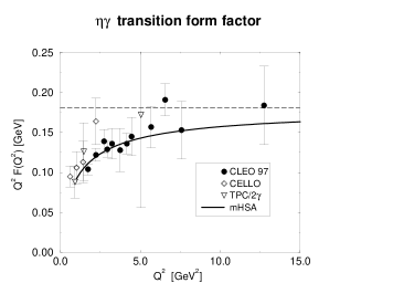
a)   b)

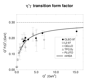
Figure 1: a) The $\eta\gamma$ transition form-factor, and b) the $\eta^{\prime}\gamma$ transition form factor, each multiplied by $Q^{2}$. The dashed lines indicate the asymptotic limit (15). The solid line is the mHSA calculation. Data are taken from Refs. [3, 12, 13, 14, 15].

             

Figure 2: Lowest order Feynman graphs contributing to the hard-scattering amplitude $T_{H}$.

The $P\gamma$ transition form factors can now be calculated from the following convolution formula

$$F_{P\gamma}(Q^{2}) = \sum_{a}\int dx\,\frac{d^{2}b}{4\pi}\,{\hat{T}_{H}^{a}(x,b,Q^{2})}\times$$ (13)

$$\ {\exp[-\mathcal{S}]}\,{\hat{\psi}_{P}^{a}(x,b)}\ .$$

A Fourier transformation to transverse configuration space, $\vec{k}_{\perp}\to\vec{b}$, has been performed which is indicated by the hat over $T_{H}^{a}$ and $\Psi_{P}^{a}$. The hard-scattering amplitude is calculated from the Feynman-graphs in Fig. 2,

$$T_{H}^{a} = \frac{4\sqrt{6}\,C_{a}}{xQ^{2}+\vec{k}_{\perp}^{2}+x(1-x)M_{P}^{2}}$$ (14)

with $C_{8}=(e_{u}^{2}+e_{d}^{2}-2e_{s}^{2})/\sqrt{6}$ and $C_{0}=(e_{u}^{2}+e_{d}^{2}+e_{s}^{2})/\sqrt{3}$ denoting charge factors. The term $\exp[-{\mathcal{S}}]$ denotes the Sudakov factor (its explicit form can be found in Ref. [16]). The transverse separation $b$ of the two quarks inside the meson provides an intrinsic definition of the (gliding) factorization scale $\mu_{F}=1/b$ which sets the interface between true non-perturbative soft gluon contributions – still contained in the hadronic wave functions – and perturbative ones accounted for by the Sudakov factor.

The integral in Eq. (13) can be calculated numerically and leads to the result shown in Fig. 1. One observes a perfect description of the experimental data for $Q^{2}\geq 1$ GeV². We also have shown the asymptotic limit of the transition form factors which follows from Eqs. (5), (13) and (14)

$$\lim_{Q^{2}\to\infty}Q^{2}\,F_{P\gamma}(Q^{2}) = \sum_{a}6\,C_{a}\,f_{P}^{a}\ .$$ (15)

Using the parameters (9), one obtains for the r.h.s. of Eq. (15) the values $181$ MeV and $299$ MeV for $\eta$ and $\eta^{\prime}$ mesons, respectively. This has to be compared with the value $185$ MeV for the $\pi^{0}$, see Eq. (2). Note that the approximate equality of the asymptotic limit for the $\pi^{0}\gamma$ and $\eta\gamma$ transition form factor is totally accidental and has nothing to do with $SU(3)_{F}$ flavor symmetry within the pseudoscalar octet (which is, of course, broken here by the electric charges).

3 Interpretation of the data

One of the conclusions drawn at the Photon’97 conference on the basis of the CLEO data for the $P\gamma$ transition form factors was that the $\eta^{\prime}$ meson behaves differently than the other light pseudoscalars [17]. Although, at first glance, this statement is not surprising since the $\eta^{\prime}$ is known to be effected by the $U(1)_{A}$ anomaly, it is in obvious contradiction to the results presented in the previous section where a good description of the data has been achieved with similar LCWFs for $\pi^{0}$, $\eta$ and $\eta^{\prime}$ mesons. The resolution of the apparent contradiction is connected with the treatment of the data at large and small values of $Q^{2}$.

First, let us plot again the large-$Q^{2}$ data from CLEO for $\pi^{0}$, $\eta$ and $\eta^{\prime}$ but now divided by their asymptotic behavior, Eqs. (2) and (15), respectively, see Fig. 3. Basically, within the errors, the data for the three different mesons fall on top of each other. For comparison, we have again included the result of the mHSA approach (13) – with meson masses neglected in the hard-scattering amplitude (14) – and also the sHSA prediction [4]

$$Q^{2}\,F_{\pi\gamma}(Q^{2}) = \sqrt{2}\,f_{\pi}\ \left(1-\frac{5}{3}\,\frac{\alpha_{V}(e^{-3/2}Q)}{\pi}\right)\ .$$

In both cases we have employed the asymptotic distribution amplitude. Note that, following Ref. [4], in Eq. (LABEL:shsa) a freezing strong coupling constant $\alpha_{V}$ is utilized at rather small renormalization scales. Both, the sHSA and the mHSA, describe the data reasonably well.

As discussed above, the $P\gamma$ transition form factor at large values of momentum transfer is dominated by the $|q\bar{q}\rangle$ Fock states. We therefore have to conclude that $\pi^{0}$, $\eta^{\prime}$ and $\eta^{\prime}$ mesons behave similarly in hard exclusive reactions due to the fact that the anomalous character of the $\eta^{\prime}$ meson does not show up in the $|q\bar{q}\rangle$ Fock states.

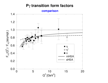
Figure 3: Comparison of $P\gamma$ transition form factors for $P=\pi^{0},\eta,\eta^{\prime}$. Data are taken from CLEO [3] and divided by the asymptotic behavior (2) and (15). The solid line is the mHSA prediction (13); the dashed line the sHSA prediction (LABEL:shsa), the dotted line the asymptotic limit. Meson masses have been neglected in this plot.

On the other hand, in experimental analyses one often performs a fit to the data which is based on a simple pole ansatz

$$F_{P\gamma}(Q^{2}) \propto \frac{1}{1+Q^{2}/\Lambda_{P}^{2}}\ .$$ (17)

The fit includes data at both, low and high values of momentum transfer. The effective pole masses found from e.g. the CLEO analysis [17] are $\Lambda_{\pi}=776\pm 22$ MeV, $\Lambda_{\eta}=774\pm 29$ MeV, and $\Lambda_{\eta^{\prime}}=859\pm 28$ MeV. Apparently, the $\eta^{\prime}$ behaves differently in that kind of analyses. But is there any deeper physical meaning in the parameters $\Lambda_{P}$? To answer this question it is necessary to consider interpolation formulas for the $P\gamma$ transition form factors which are usually taken as a justification of Eq. (17). For the pion such a simple formula has been proposed by Brodsky/Lepage [1]

$$F_{\pi\gamma}^{BL}(Q^{2}) = \frac{\sqrt{2}\,f_{\pi}}{Q^{2}+4\pi^{2}f^{2}_{\pi}}\ .$$ (18)

Obviously, it has the correct asymptotic limit (2). Furthermore for $Q^{2}\to 0$ it coincides with the chiral anomaly prediction. Eqs. (18) and (17) also happen to have a similar form as the vector dominance model (VDM). One also has the approximate equality $\Lambda_{\pi}\simeq 2\pi f_{\pi}\simeq M_{\rho,\omega}$, but there is no reason for these relations to be exact.

Things become more involved if we consider the $\eta\gamma$ and $\eta^{\prime}\gamma$ transition form factors. Here both, the asymptotic limit (15) as well as the chiral anomaly prediction for $Q^{2}=0$ [8, 7] are given by a linear combination of two terms, arising from the mixing of octet and singlet contributions. For $\theta_{8}\neq\theta_{0}$ the pre-factors in the limit $Q^{2}\to 0$ and $Q^{2}\to\infty$ are different, and one does not find a simple interpolation formula. It has been observed [9] that the decay constants which enter both the theoretical predictions, for $Q^{2}=0$ and $Q^{2}\to\infty$, have (at least approximately) a much simpler decomposition in the quark flavor basis,

$$\left(\matrix{f_{\eta}^{q}&f_{\eta}^{s}\vspace{0.2em}\cr f_{\eta^{\prime}}^{q}&f_{\eta^{\prime}}^{s}}\right) = \left(\matrix{f_{q}\,\cos\phi&-f_{s}\,\sin\phi\vspace{0.2em}\cr f_{q}\,\sin\phi&\phantom{-}f_{s}\,\cos\phi}\right)\ .$$ (19)

Here the index $q$ denotes the flavor combination $(u\bar{u}+d\bar{d})/\sqrt{2}$ and $s$ stands for $s\bar{s}$. The parameters in Eq. (9) correspond to $\phi=39.3^{\circ}$, $f_{q}=1.07\,f_{\pi}$, $f_{s}=1.36\,f_{\pi}$. In the quark flavor basis it is sufficient to consider only one single mixing angle $\phi$. This is equivalent to neglecting all true OZI-rule violating contributions while topological effects connected to the $U(1)_{A}$ anomaly and mixing are kept. In this scheme interpolation formulas can be obtained [7] as a linear combination of two individual terms which resemble the Brodsky/Lepage formula

$$F_{P\gamma}^{\rm int}(Q^{2}) = \sum_{i=q,s}\frac{6\,C_{i}\,f_{P}^{i}}{Q^{2}+4\pi^{2}\,f_{i}^{2}}\ ,\qquad(P=\eta,\eta^{\prime})$$

with $C_{q}=5/9\sqrt{2}$ and $C_{s}=1/9$. Again we have an approximate relation to VDM, since $M_{\rho,\omega}\simeq 2\pi f_{q}$ and $M_{\phi}\simeq 2\pi f_{s}$. A simple connection to the experimental fit parameters $\Lambda_{\eta}$ and $\Lambda_{\eta^{\prime}}$ can, however, not be found. We may expect that the values of $\Lambda_{\eta}$ and $\Lambda_{\eta^{\prime}}$ lie somehow between $M_{\rho}$ and $M_{\phi}$. In fact, since the charge factor in front of the strange quark contribution in Eq. (LABEL:etainterpolqs) is smaller than the one for the light quark contribution the values of $\Lambda_{P}$ should be closer to the $\rho$ mass. Furthermore, for $\phi=39.3^{\circ}$ the strange quark component of the $\eta^{\prime}$ meson is larger than the one for $\eta$; thus one should have $\Lambda_{\eta^{\prime}}>\Lambda_{\eta}$. This is in line with the experimental findings.

Coming back to our question from above, we have to consider the pole-parameters $\Lambda_{P}$ as an effective way to compare results of different experiments (as long as they are performed at similar values of $Q^{2}$). They have no deeper theoretical meaning, although they show some qualitative similarities with VDM. In particular, the values of $\Lambda_{P}$ cannot be used as a measurement of the decay constants $f_{\pi}$ and $f_{P}^{a}$.

Furthermore, interpolation formulas like Eqs. (18), (LABEL:etainterpolqs) have to be used with some care: Compared to the mHSA prediction they tend to overestimate the transition form factor at intermediate momentum transfer [7]. Nevertheless, they can be used to obtain a rough estimate, e.g. for the implementation of the transition form factors in Monte Carlo generators [18].

If both photons are taken far off-shell one should also keep in mind that the naive VDM-prediction leads to the wrong asymptotic behavior ($\propto 1/Q_{1}^{2}Q_{2}^{2}$). The correct limit is obtained from a generalization of Eq. (15)

$$\lim_{Q_{1}^{2},Q_{2}^{2}\to\infty}\,F_{P\gamma^{*}}(Q_{1}^{2},Q_{2}^{2})$$

$$= \sum_{i=q,s}6\,C_{i}\,f_{P}^{i}\,\int_{0}^{1}dx\,\frac{2x(1-x)}{xQ_{1}^{2}+(1-x)Q_{2}^{2}}\ .$$

Starting from Eq. (LABEL:gammastarlimit), again interpolation formulas for the general case $Q_{1}^{2},Q_{2}^{2}\neq 0$ can be constructed. A simple choice, which leads to results that are very close to the mHSA calculation, is to perform in Eq. (LABEL:gammastarlimit) the replacement,

$$xQ_{1}^{2}+(1-x)Q_{2}^{2}\to xQ_{1}^{2}+(1-x)Q_{2}^{2}+4\pi^{2}f_{i}^{2}/3\ .$$

The $x$-integration in Eq. (LABEL:gammastarlimit) can be performed analytically, but the result looks rather complicated. For a further discussion and alternative choices of interpolation formulas see also the work of Ong [19] which has been contributed to the Photon’97 conference. In any case, for the interpolation formulas for $P\gamma^{*}$ transition form factors the same limitations apply as for the approximations (18) and (LABEL:etainterpolqs).

4 Conclusions

The experimental data for $\eta\gamma$ and $\eta^{\prime}\gamma$ transition form factors at large momentum transfer are well described by the hard-scattering approach. Two important features of $\eta$ and $\eta^{\prime}$ mesons can be read off from the data: i) The distribution amplitudes of the quark-antiquark Fock states of $\eta$ and $\eta^{\prime}$ mesons are similar to the pion one and close to the asymptotic form already at low scales. This means that the $U(1)_{A}$ anomaly does not show up in the shape of the LCWFs of the valence Fock states. A similar conclusion has been drawn within a somewhat different framework in Ref. [20]. ii) The values of the decay constants in the $\eta$-$\eta^{\prime}$ system, which have been determined from a detailed phenomenological analysis elsewhere [9], are confirmed. This underlines the necessity of using the general mixing scheme presented in Ref. [8] whereas a description in terms of a single octet-singlet mixing angle is disfavored.

The interpretation of the experimental data by means of effective pole masses based on simplified interpolation formulas can be very misleading and has to be considered with great care. At most, such a procedure can be used to compare different experiments, provided that the data is taken within similar ranges of momentum transfer. The pole masses do not at all provide a process-independent definition of ‘decay constants’.

The results can easily be generalized to the case where both photons are off-shell. Experimental data for $P\gamma^{*}$ transition form factors is, however, not available yet.

References

-
[1]
G. P. Lepage and S. J. Brodsky,
Phys. Rev. D22, 2157 (1980),
S.J. Brodsky and G.P. Lepage, Phys. Rev. D24 1808 (1981). - [2] A. V. Efremov and A. V. Radyushkin, Phys. Lett. 94B, 245 (1980).
- [3] CLEO collab., J. Gronberg et al., Phys. Rev. D57, 33 (1998).
- [4] S. J. Brodsky, hep-ph/9708345, Proceedings of Photon ’97, Egmond aan Zee 1997, Eds.: A. Buijs and F.C. Erné.
-
[5]
R. Jakob, P. Kroll and M. Raulfs,
J. Phys. G22, 45 (1996);
P. Kroll and M. Raulfs, Phys. Lett. B387, 848 (1996). - [6] I. V. Musatov and A. V. Radyushkin, Phys. Rev. D56, 2713 (1997).
- [7] T. Feldmann and P. Kroll, Eur. Phys. J. C5, 327 (1998), Phys. Rev. D58:057501 (1998).
-
[8]
H. Leutwyler,
Nucl. Phys. Proc. Suppl. 64, 223 (1998),
R. Kaiser and H. Leutwyler, hep-ph/9806336,
R. Kaiser, diploma work, Bern University 1997. - [9] T. Feldmann, P. Kroll, and B. Stech, Phys. Rev. D58, 114006 (1998), Phys. Lett. B449, 339 (1999).
- [10] M. Diehl, T. Feldmann, R. Jakob, and P. Kroll, Eur. Phys. J. C8, 409 (1999),
- [11] S. J. Brodsky, T. Huang, and G. P. Lepage, Particles and Fields 2, eds. Z.Capri and A.N. Kamal (Banff Summer Institute, 1983) 143.
- [12] L3 collab., M. Acciarri et al., Phys. Lett. B418, 399 (1998).
- [13] CELLO collab., H. J. Behrend et al., Z. Phys. C49, 401 (1991).
- [14] TPC/2 collab., H. Aihara et al., Phys. Rev. Lett. 64, 172 (1990).
- [15] PLUTO collab., C. Berger et al., Phys. Lett. 142B, 125 (1984).
- [16] M. Dahm, R. Jakob, and P. Kroll, Z. Phys. C68, 595 (1995).
- [17] CLEO collab., V. Savinov, hep-ex/9707028, Proceedings of Photon ’97, Egmond aan Zee 1997, Eds.: A. Buijs and F.C. Erné.
- [18] R. van Gulik, Talk presented at this conference.
- [19] S. Ong, Phys. Rev. D52, 3111 (1995), and in Proceedings of Photon ’97, Egmond aan Zee 1997, Eds.: A. Buijs and F.C. Erné.
- [20] V. V. Anisovich, D. I. Melikhov, and V. A. Nikonov, Phys. Rev. D55, 2918 (1997).