Neutrino Mass: theory, data and interpretation

Abstract:

In these two lectures I describe first the theory of neutrino mass and then discuss the implications of recent data (including 708–day data Super–Kamiokande data) which strongly indicate the need for neutrino conversions to account for the solar and atmospheric neutrino observations. I also mention the LSND data, which provides an intriguing hint. The simplest ways to reconcile all these data in terms of neutrino oscillations invoke a light sterile neutrino in addition to the three active ones. Out of the four neutrinos, two are maximally-mixed and lie at the LSND scale, while the others are at the solar mass scale. These schemes can be distinguished at neutral-current-sensitive solar & atmospheric neutrino experiments. I discuss the simplest theoretical scenarios, where the lightness of the sterile neutrino, the nearly maximal atmospheric neutrino mixing, and the generation of $\Delta{m^{2}}_{\odot}$ & $\Delta{m^{2}}_{atm}$ all follow naturally from the assumed lepton-number symmetry and its breaking. Although the most likely interpretation of the present data is in terms of neutrino-mass-induced oscillations, one still has room for alternative explanations, such as flavour changing neutrino interactions, with no need for neutrino mass or mixing. Such flavour violating transitions arise in theories with strictly massless neutrinos, and may lead to other sizeable flavour non-conservation effects, such as $\mu\to e+\gamma$, $\mu-e$ conversion in nuclei, unaccompanied by neutrino-less double beta decay.

1 Introduction

Since the early geochemical experiments of Davis and collaborators, underground experiments have by now provided solid evidence for the solar and the atmospheric neutrino problems, the two milestones in the search for physics beyond the Standard Model (SM)  [1, 2, 3, 4, 5, 6, 7]. Of particular importance has been the recent confirmation by the Super-Kamiokande collaboration [3] of the atmospheric neutrino zenith angle dependent deficit, which has marked a turning point in our understanding of neutrinos, providing a strong evidence for $\nu_{\mu}$ conversions. In addition to the neutrino data from underground experiments there is also some indication for neutrino oscillations from the LSND experiment [8, 9].

Neutrino conversions are naturally expected to take place if neutrinos are massive, as expected in most extensions of the Standard Model [10]. The preferred theoretical origin of neutrino mass is lepton number violation, which typically leads also to lepton flavour violating transitions such as neutrino-less double beta decay, so far unobserved. However, lepton flavour violating transitions may arise without neutrino masses  [11, 12] in models with extra heavy leptons [13, 14] and in supergravity  [15]. Indeed the atmospheric neutrino anomaly can be explained in terms of flavour changing neutrino interactions, with no need for neutrino mass or mixing [16]. Whether or not this mechanism will resist the test of time it will still remain as one of the ingredients of the final solution, at the moment not required by the data. A possible signature of theories leading to FC interactions would be the existence of sizeable flavour non-conservation effects, such as $\mu\to e+\gamma$, $\mu-e$ conversion in nuclei, unaccompanied by neutrino-less double beta decay. In contrast to the intimate relationship between the latter and the non-zero Majorana mass of neutrinos due to the Black-Box theorem [17] there is no fundamental link between lepton flavour violation and neutrino mass. Barring such exotic mechanisms reconciling the LSND (and possibly Hot Dark Matter, see below) together with the data on solar and atmospheric neutrinos requires three mass scales. The simplest way is to invoke the existence of a light sterile neutrino [18, 19, 20]. Out of the four neutrinos, two of them lie at the solar neutrino scale and the other two maximally-mixed neutrinos are at the HDM/LSND scale. The prototype models proposed in [18, 19] enlarge the $SU(2)\otimes U(1)$ Higgs sector in such a way that neutrinos acquire mass radiatively, without unification nor seesaw. The LSND scale arises at one-loop, while the solar and atmospheric scales come in at the two-loop level, thus accounting for the hierarchy. The lightness of the sterile neutrino, the nearly maximal atmospheric neutrino mixing, and the generation of the solar and atmospheric neutrino scales all result naturally from the assumed lepton-number symmetry and its breaking. Either $\nu_{e}$ - $\nu_{\tau}$ conversions explain the solar data with $\nu_{\mu}$ - $\nu_{s}$ oscillations accounting for the atmospheric deficit [18], or else the rôles of $\nu_{\tau}$ and $\nu_{s}$ are reversed  [19]. These two basic schemes have distinct implications at future solar & atmospheric neutrino experiments with good sensitivity to neutral current neutrino interactions. Cosmology can also place restrictions on these four-neutrino schemes.

2 Mechanisms for Neutrino Mass

Why are neutrino masses so small compared to those of the charged fermions? Because of the fact that neutrinos, being the only electrically neutral elementary fermions should most likely be Majorana, the most fundamental fermion. In this case the suppression of their mass could be associated to the breaking of lepton number symmetry at a very large energy scale within a unification approach, which can be implemented in many extensions of the SM. Alternatively, neutrino masses could arise from garden-variety weak-scale physics specified by a scale $\left\langle\sigma\right\rangle=\hbox{$\cal O$ }(m_{Z})$ where $\left\langle\sigma\right\rangle$ denotes a $SU(2)\otimes U(1)$ singlet vacuum expectation value which owes its smallness to the symmetry enhancement which would result if $\left\langle\sigma\right\rangle$ and $m_{\nu}\to 0$.

One should realize however that, the physics of neutrinos can be rather different in various gauge theories of neutrino mass, and that there is hardly any predictive power on masses and mixings, which should not come as a surprise, since the problem of mass in general is probably one of the deepest mysteries in present-day physics.

2.1 Unification or Seesaw Neutrino Masses

The observed violation of parity in the weak interaction may be a reflection of the spontaneous breaking of B-L symmetry in the context of left-right symmetric extensions such as the $SU(2)_{L}\otimes SU(2)_{R}\otimes U(1)$[21], $SU(4)\otimes SU(2)\otimes SU(2)$ [22] or $SO(10)$ gauge groups [23]. In this case the masses of the light neutrinos are obtained by diagonalizing the following mass matrix in the basis $\nu,\nu^{c}$

$$\left[\matrix{M_{L}&D\cr D^{T}&M_{R}}\right]$$ (1)

where $D$ is the standard $SU(2)\otimes U(1)$ breaking Dirac mass term and $M_{R}=M_{R}^{T}$ is the isosinglet Majorana mass that may arise from a 126 vacuum expectation value in $SO(10)$. The magnitude of the $M_{L}\nu\nu$ term [24] is also suppressed by the left-right breaking scale, $M_{L}\propto 1/M_{R}$ [21]. In the seesaw approximation, one finds

$$M_{\nu\>eff}=M_{L}-DM_{R}^{-1}D^{T}\>.$$ (2)

As a result one is able to explain naturally the relative smallness of neutrino masses since $m_{\nu}\propto 1/M_{R}$. Although $M_{R}$ is expected to be large, its magnitude heavily depends on the model and it may have different possible structures in flavour space (so-called textures) [25]. In general one can not predict the corresponding light neutrino masses and mixings. In fact this freedom has been exploited in model building in order to account for an almost degenerate seesaw-induced neutrino mass spectrum [26].

One virtue of the unification approach is that it may allow one to gain a deeper insight into the flavour problem. There have been interesting attempts at formulating supersymmetric unified schemes with flavour symmetries and texture zeros in the Yukawa couplings. In this context a challenge is to obtain the large lepton mixing now indicated by the atmospheric neutrino data.

2.2 Weak-Scale Neutrino Masses

Neutrinos may acquire mass from extra particles with masses $\hbox{$\cal O$ }(m_{Z})$ an therefore accessible to present experiments. There is a variety of such mechanisms, in which neutrinos acquire mass either at the tree level or radiatively. Let us look at some examples, starting with the tree level case.

2.2.1 Tree-level Neutrino Masses

Consider the following extension of the lepton sector of the $SU(2)\otimes U(1)$ theory: let us add a set of $two$ 2-component isosinglet neutral fermions, denoted ${\nu^{c}}_{i}$ and $S_{i}$, $i=e,~{}\mu$ or $\tau$ in each generation. In this case one can consider the mass matrix (in the basis $\nu,\nu^{c},S$) [27]

$$\left[\matrix{0&D&0\cr D^{T}&0&M\cr 0&M^{T}&\mu}\right]$$ (3)

The Majorana masses for the neutrinos are determined from

$$M_{L}=DM^{-1}\mu{M^{T}}^{-1}D^{T}$$ (4)

In the limit $\mu\to 0$ the exact lepton number symmetry is recovered and will keep neutrinos strictly massless to all orders in perturbation theory, as in the SM. The corresponding texture of the mass matrix has been suggested in various theoretical models [13], such as superstring inspired models [14]. In the latter the zeros arise due to the lack of Higgs fields to provide the usual Majorana mass terms. The smallness of neutrino mass then follows from the smallness of $\mu$. The scale characterizing $M$, unlike $M_{R}$ in the seesaw scheme, can be low. As a result, in contrast to the heavy neutral leptons of the seesaw scheme, those of the present model can be light enough as to be produced at high energy colliders such as LEP [28] or at a future Linear Collider. The smallness of $\mu$ is in turn natural, in t’Hooft’s sense, as the symmetry increases when $\mu\to 0$, i.e. total lepton number is restored. This scheme is a good alternative to the smallness of neutrino mass, as it bypasses the need for a large mass scale, present in the seesaw unification approach. One can show that, since the matrices $D$ and $M$ are not simultaneously diagonal, the leptonic charged current exhibits a non-trivial structure that cannot be rotated away, even if we set $\mu\equiv 0$. The phenomenological implication of this, otherwise innocuous twist on the SM, is that there is neutrino mixing despite the fact that light neutrinos are strictly massless. It follows that flavour and CP are violated in the leptonic currents, despite the masslessness of neutrinos. The loop-induced lepton flavour and CP non-conservation effects, such as $\mu\to e+\gamma$ [11, 12], or CP asymmetries in lepton-flavour-violating processes such as $Z\to e\bar{\tau}$ or $Z\to\tau\bar{e}$ [29] are precisely calculable. The resulting rates may be of experimental interest [30, 31, 32], since they are not constrained by the bounds on neutrino mass, only by those on universality, which are relatively poor. In short, this is a conceptually simple and phenomenologically rich scheme.

Another remarkable implication of this model is a new type of resonant neutrino conversion mechanism [33], which was the first resonant mechanism to be proposed after the MSW effect [34], in an unsuccessful attempt to bypass the need for neutrino mass in the resolution of the solar neutrino problem. According to the mechanism, massless neutrinos and anti-neutrinos may undergo resonant flavour conversion, under certain conditions. Though these do not occur in the Sun, they can be realized in the chemical environment of supernovae [35]. Recently it has been pointed out how they may provide an elegant approach for explaining the observed velocity of pulsars [36].

2.2.2 Radiative Neutrino Masses

The prototype one-loop scheme is the one proposed by Zee [37]. Supersymmetry with explicitly broken R-parity also provides alternative one-loop mechanisms to generate neutrino mass arising from scalar quark or scalar lepton exchanges, as shown in Fig. (1).

Figure 1: Mechanism for One-loop-induced Neutrino Mass.

An interesting two-loop scheme to induce neutrino masses was suggested by Babu [38], based on the diagram shown in Fig. (2).

Figure 2: Mechanism for Two-loop-induced Neutrino Mass

Note that I have used here a slight variant of the original model which incorporates the idea of spontaneous [39], rather than explicit lepton number violation.

Finally, note also that one can combine these mechanisms as building blocks in order to provide schemes for massive neutrinos. In particular those in which there are not only the three active neutrinos but also one or more light sterile neutrinos, such as those in ref. [18, 19]. In fact this brings in novel Feynman graph topologies.

2.3 Supersymmetry: R-parity Violation as the Origin of Neutrino Mass

This is an interesting mechanism of neutrino mass generation which combines seesaw and radiative mechanisms [40]. It invokes supersymmetry with broken R-parity, as the origin of neutrino mass and mixings. The simplest way to illustrate the idea is to use the bilinear breaking of R–parity [40, 41] in a unified minimal supergravity scheme with universal soft breaking parameters (MSUGRA). Contrary to a popular misconception, the bilinear violation of R–parity implied by the $\epsilon_{3}$ term in the superpotential is physical, and can not be rotated away [42]. It leads also by a minimization condition, to a non-zero sneutrino vev, $v_{3}$. It is well-known that in such models of broken R–parity the tau neutrino $\nu_{\tau}$ acquires a mass, due to the mixing between neutrinos and neutralinos [43]. It comes from the matrix

$$\left[\matrix{M_{1}&0&-{1\over 2}g^{\prime}v_{d}&{1\over 2}g^{\prime}v_{u}&-{1\over 2}g^{\prime}v_{3}\cr 0&M_{2}&{1\over 2}gv_{d}&-{1\over 2}gv_{u}&{1\over 2}gv_{3}\cr-{1\over 2}g^{\prime}v_{d}&{1\over 2}gv_{d}&0&-\mu&0\cr{1\over 2}g^{\prime}v_{u}&-{1\over 2}gv_{u}&-\mu&0&\epsilon_{3}\cr-{1\over 2}g^{\prime}v_{3}&{1\over 2}gv_{3}&0&\epsilon_{3}&0}\right]$$ (5)

where the first two rows are gauginos, the next two Higgsinos, and the last one denotes the tau neutrino. The $v_{u}$ and $v_{d}$ are the standard vevs, $g^{\prime}s$ are gauge couplings and $M_{1,2}$ are the gaugino mass parameters. Since the $\epsilon_{3}$ and the $v_{3}$ are related, the simplest (one-generation) version of this model contains only one extra free parameter in addition to those of the MSUGRA model. The universal soft supersymmetry-breaking parameters at the unification scale $m_{X}$ are evolved via renormalization group equations down to the weak scale $\hbox{$\cal O$ }(m_{Z})$. This induces an effective non-universality of the soft terms at the weak scale which in turn implies a non-zero sneutrino vev $v^{\prime}_{3}$ given as

$$v^{\prime}_{3}\approx\frac{\epsilon_{3}\mu}{{m_{Z}}^{4}}\left(v^{\prime}_{d}\Delta M^{2}+\mu^{\prime}v_{u}\Delta B\right)$$ (6)

where the primed quantities refer to a basis in which we eliminate the $\epsilon_{3}$ term from the superpotential (but reintroduce it, of course, in other sectors of the theory).

The scalar soft masses and bilinear mass parameters obey $\Delta M^{2}=0$ and $\Delta B=0$ at $m_{X}$. However at the weak scale they are calculable from radiative corrections as

$$\Delta M^{2} \approx {{3h_{b}^{2}}\over{8\pi^{2}}}m_{Z}^{2}\ln{{M_{GUT}}\over{m_{Z}}}$$ (7)

Note that eq. (6) implies that the R–parity-violating effects induced by $v^{\prime}_{3}$ are calculable in terms of the primordial R–parity-violating parameter $\epsilon_{3}$. It is clear that the universality of the soft terms plays a crucial rôle in the calculability of the $v^{\prime}_{3}$ and hence of the resulting neutrino mass [40]. Thus eq. (5) represents a new kind of see-saw scheme in which the $M_{R}$ of eq. (1) is the neutralino mass, while the rôle of the Dirac entry $D$ is played by the $v^{\prime}_{3}$, which is induced radiatively as the parameters evolve from $m_{X}$ to the weak scale. Thus we have a hybrid see-saw mechanism, with naturally suppressed Majorana $\nu_{\tau}$ mass induced by the mixing between the weak eigenstate tau neutrino and the zino.

In order to estimate the expected $\nu_{\tau}$ mass let me first determine the tau neutrino mass in the most general supersymmetric model with bilinear breaking of R-parity, without imposing universality of the soft SUSY breaking terms. The $\nu_{\tau}$ mass depends quadratically on an effective parameter $\xi$ defined as $\xi\equiv(\epsilon_{3}v_{d}+\mu v_{3})^{2}\propto{v^{\prime}_{3}}^{2}$ characterizing the violation of R–parity. The expected $m_{\nu_{\tau}}$ values are illustrated in Fig. (3). The band shown in the figure is obtained through a scan over the parameter space requiring that the supersymmetric particles are not too light.

Figure 3: Tau neutrino mass from Broken R–parity vs $\xi\equiv(\epsilon_{3}v_{d}+\mu v_{3})^{2}$ from ref. [40].

This should be compared with the cosmologically allowed values of the tau neutrino mass $\sum m_{\nu}\raise 1.29167pt\hbox{$\;<$\kern-7.5pt\raise-4.73611pt\hbox{$\sim\;$}}92\Omega h^{2}$ eV (see below). Note that this only holds if neutrinos are stable. In the present model the $\nu_{\tau}$ is expected to decay into 3 neutrinos, via the neutral current [24, 44], or by slepton exchanges. This decay will reduce the relic $\nu_{\tau}$ abundance to the required level, as long as $\nu_{\tau}$ is heavier than about 200 KeV or so. Since on the other hand primordial Big-Bang nucleosynthesis implies that $\nu_{\tau}$ is lighter than about an MeV or so [45] there is a forbidden gap in this model if the majoron is not introduced. In the full version of the model the presence of the majoron allows all neutrino masses to be viable cosmologically.

Back to the simplest model with explicit bilinear breaking of R–parity, let me note that in this model the $\nu_{\tau}$ mass can be very large. A way to obtain a model with a small and calculable $\nu_{\tau}$ mass, as indicated by the simplest interpretation of the atmospheric neutrino anomaly in terms of $\nu_{\mu}$ to $\nu_{\tau}$ oscillations is to assume a SUGRA scheme with universality of the soft supersymmetry breaking terms at $m_{X}$. In this case the $\nu_{\tau}$ mass is theoretically predicted in terms of $h_{b}$ and can be small in this case due to a natural cancellation between the two terms in the parameter $\xi$, which follows from the assumed universality of the soft terms at $m_{X}$. One can verify that $m_{\nu_{\tau}}$ may easily lie in the ten electron-volt range. Lower masses require about two orders of magnitude in addition to that which is dictated by the RGE evolution, which is certainly not unreasonable. Moreover the solution of the atmospheric neutrino anomaly may involve some exotic mechanism, such as the FC interactions [16].

As a last remark I note that $\nu_{e}$ and $\nu_{\mu}$ remain massless in this approximation. They get masses either from scalar loop contributions in Fig. (1) or by mixing with singlets in models with spontaneous breaking of R-parity [46]. A detailed study is now underway of the loop contributions to $\nu_{\mu}$ and $\nu_{e}$ is underway in Valencia. It is important to notice that even when $m_{\nu_{\tau}}$ is small, many of the corresponding R-parity violating effects can be sizeable. An obvious example is the fact that the lightest neutralino decay will typically decay inside the detector, unlike standard R-parity-conserving supersymmetry. This leads to a vastly unexplored plethora of phenomenological possibilities in supersymmetric physics [47].

In conclusion one can see that, of the various attractive schemes for giving neutrinos a mass, only the seesaw scheme requires a large mass scale. It gives a grand connection between the very light (the neutrinos) and the very heavy (some unknown particles). At this stage is is premature to bet on any mechanism and from this point of view neutrinos open the door to a potentially rich phenomenology, since the extra particles required have masses at scales that could be accessible to present experiments. In the simplest versions of these models the neutrino mass arises from the explicit violation of lepton number. Their phenomenological potential gets even richer if one generalizes the models so as to implement a spontaneous violation scheme. This brings me to the next section.

2.4 Majorons at the Weak-scale

The generation of neutrino masses will be accompanied by the existence of a physical Goldstone boson that we generically call majoron in any model where lepton number (or B-L) is an ungauged symmetry which is arranged to break spontaneously. Except for the left-right symmetric unification approach, in which B-L is a gauge symmetry, in all of the above schemes one can implement the spontaneous violation of lepton number. One can also introduce it in a seesaw framework, both with $SU(2)\otimes U(1)$ [48] as well as left-right symmetry [49]. While in the $SU(2)\otimes U(1)$ case it is rather simple, in the case of left-right-symmetric models, one needs to implement a spontaneously broken global U(1) symmetry similar to lepton number. One interesting aspect that emerges in the latter case is that it allows also the left-right scale to be relatively low [49]. Here I do not consider the seesaw-type majorons, for a discussion see ref. [10]. I will mainly concentrate on weak-scale physics. In all models I consider the lepton-number breaks at a scale given by a vacuum expectation value $\left\langle\sigma\right\rangle\sim m_{weak}$. In all of these models, the weak scale arises as the most natural one and, as already mentioned, the neutrino masses when $\left\langle\sigma\right\rangle\to 0$ i.e. when the lepton-breaking scale vanish [50].

In any phenomenologically acceptable model one must arrange for the majoron to be mainly an $SU(2)\otimes U(1)$ singlet, ensuring that it does not affect the invisible Z decay width, well-measured at LEP. In models where the majoron has L=2 the neutrino mass is proportional to an insertion of $\left\langle\sigma\right\rangle$, as indicated in Fig. (2). In the supersymmetric model with broken R-parity the majoron is mainly a singlet sneutrino, which has lepton number L=1, so that $m_{\nu}\propto\left\langle\sigma\right\rangle^{2}$, where $\left\langle\sigma\right\rangle\equiv\left\langle\widetilde{\nu^{c}}\right\rangle$, with $\widetilde{\nu^{c}}$ denoting the singlet sneutrino. The presence of the square, just as in the parameter $\xi$  in Fig. (3), reflects the fact that the neutrino gets a Majorana mass which has lepton number L=2. The sneutrino gets a vev at the effective supersymmetry breaking scale $m_{susy}=m_{weak}$.

The weak-scale majorons may have other phenomenological implications. One is the possibility of invisibly decaying Higgs bosons [50] which I have no time to discuss here (see, for instance [47]).

Finally note that if the majoron acquires a KeV mass (natural in weak-scale models) from gravitational effects at the Planck scale [51] it may play obey the main requirements to play a rôle in cosmology as dark matter [52]. In what follows I will just focus on two examples of how the underlying physics of weak-scale majoron models can affect neutrino cosmology in an important way.

2.4.1 Heavy Neutrinos and the Universe Mass

Neutrinos of mass less than $\cal O$ (100 KeV) or so, are cosmologically stable if they have only SM interactions. Their contribution to the present density of the universe implies [53]

$$\sum m_{\nu_{i}}\raise 1.29167pt\hbox{$\;<$\kern-7.5pt\raise-4.73611pt\hbox{$\sim\;$}}92\>\Omega_{\nu}h^{2}\>eV\>,$$ (8)

where the sum is over all isodoublet neutrino species with mass less than $\cal O$ (1 MeV). The parameter $\Omega_{\nu}h^{2}\leq 1$, where $h^{2}$ measures the uncertainty in the present value of the Hubble parameter, $0.4\raise 1.29167pt\hbox{$\;<$\kern-7.5pt\raise-4.73611pt\hbox{$\sim\;$}}h\raise 1.29167pt\hbox{$\;<$\kern-7.5pt\raise-4.73611pt\hbox{$\sim\;$}}1$, while $\Omega_{\nu}=\rho_{\nu}/\rho_{c}$, measures the fraction of the critical density $\rho_{c}$ in neutrinos. For the $\nu_{\mu}$ and $\nu_{\tau}$ this bound is much more stringent than the laboratory limits.

In weak-scale majoron models the generation of neutrino mass is accompanied by the existence of a physical majoron, which leads to potentially fast majoron-emitting decay channels such as [10, 54]

$$\nu^{\prime}\to\nu+J\>\>.$$ (9)

as well as new annihilations to majorons,

$$\nu^{\prime}+\nu^{\prime}\to J+J\>\>.$$ (10)

These could eliminate relic neutrinos and therefore allow neutrinos of higher mass, as long as the rates are large enough to allow for an adequate red-shift of the heavy neutrino decay and/or annihilation products. While the annihilation involves a diagonal majoron-neutrino coupling $g$, the decays proceed only via the non-diagonal part of the coupling, in the physical mass basis. A careful diagonalization of both mass matrix and coupling matrix is essential in order to avoid wild over-estimates of the heavy neutrino decay rates, such as that in ref. [48]. The point is that, once the neutrino mass matrix is diagonalized, there is a danger of simultaneously diagonalizing the majoron couplings to neutrinos. That would be analogous to the GIM mechanism present in the SM for the couplings of the Higgs to fermions. Models that avoid this GIM mechanism in the majoron-neutrino couplings have been proposed, e.g. in ref. [54]. Many of them are weak-scale majoron models [27, 46, 50]. A general method to determine the majoron couplings to neutrinos and hence the neutrino decay rates in any majoron model was first given in ref. [44]. For an estimate in the model with spontaneously broken R-parity [55] see ref. [46].

One can summarize that since neutrinos can be short-lived their masses can only be really constrained by laboratory experiments based on direct search. The cosmological and other bounds are important but require additional theoretical elements in their interpretation.

2.4.2 Heavy Neutrinos and Cosmological Nucleosynthesis

The number of light neutrino species is restricted by cosmological Big Bang Nucleosynthesis (BBN). Due to its large mass, an MeV stable (lifetime longer than $\sim 100$ sec) tau neutrino would be equivalent to several SM massless neutrino species and would therefore substantially increase the abundance of primordially produced elements, e.g. ${}^{4}He$ and deuterium [56, 57, 58, 59]. This can be converted into restrictions on the $\nu_{\tau}$ mass. If the bound on the effective number of massless neutrino species is taken as $N_{\nu}<3.4-3.6$, one can rule out $\nu_{\tau}$ masses above 0.5 MeV [45]. If we take $N_{\nu}<4.5$ [58] the $m_{\nu_{\tau}}$ limit loosens accordingly, as seen from Fig. (4), and allows a $\nu_{\tau}$ of about an MeV or so.

In the presence of $\nu_{\tau}$ annihilations the BBN $m_{\nu_{\tau}}$ bound is substantially weakened or eliminated [60]. In Fig. (4) we also give the expected $N_{\nu}$ value for different values of the coupling $g$ between $\nu_{\tau}$’s and $J$’s, expressed in units of $10^{-5}$.

Figure 4: Effective number of massless SM neutrinos equivalent to the heavy $\nu_{\tau}$ , as given in ref. [60]. Non-zero $g$ values (in units of $10^{-5}$) can lower $N_{\nu}$ with respect to the SM case $g=0$ (dashed line) due to the effect of annihilations.

Comparing with the SM $g=0$ case one sees that for a fixed $N_{\nu}^{max}$, a wide range of tau neutrino masses is allowed for large enough values of $g$. No $\nu_{\tau}$ masses below the LEP limit can be ruled out, as long as $g$ exceeds a few times $10^{-4}$. One can also see from the figure that $N_{\nu}$ can also be lowered below the canonical SM value $N_{\nu}=3$ due to the effect of the heavy $\nu_{\tau}$ annihilations to majorons. These results may be re-expressed in the $m_{\nu_{\tau}}-g$ plane, as shown in figure 5.

Figure 5: The BBN-allowed regions for each $N_{\nu}^{max}$ lie above the respective curve [60]

We note that the required values of $g(m_{\nu_{\tau}})$ fit well with the theoretical expectations of many weak-scale majoron models.

As we have seen $\nu_{\tau}$ annihilations to majorons may weaken or even eliminate the BBN constraint on the tau neutrino mass. Similarly, in some weak-scale majoron models decays in eq. (9) may lead to short enough $\nu_{\tau}$ lifetimes that they may also play an important rôle in BBN, again with the possibility of substantially weakening or eliminating the BBN constraint on the tau neutrino mass [61].

3 Indications for New Physics

The most solid hints in favour of new physics in the neutrino sector come from underground experiments on solar and atmospheric neutrinos. The published data [62, 63, 64] data correspond to a 504–day solar neutrino data sample [5] and 535–day atmospheric neutrino data sample [3], respectively. These were the data first presented at the past Neutrino 98 conference in Japan. Here we include also some results from the more recent 708–day data sample, see ref. [6] and [7].

3.1 Solar Neutrinos

The data collected by the Kamiokande, and the radiochemical Homestake, Gallex and Sage experiments have no Standard Model explanation. The event rates are summarized as: $2.56\pm 0.23$ SNU (chlorine), $72.2\pm 5.6$ SNU (Gallex and Sage gallium experiments sensitive to the $pp$ neutrinos), and $(2.44\pm 0.10)\times 10^{6}{\rm cm^{-2}s^{-1}}$ (⁸B flux from Super-Kamiokande) [1].

Figure 6: SSM predictions, from ref. [66]

In Fig. (6) one can see the predictions of various standard solar models in the plane defined by the ⁷Be and ⁸B neutrino fluxes, normalized to the predictions of the BP98 solar model [65]. Abbreviations such as BP95, identify different solar models, as given in ref. [67]. The rectangular error box gives the $3\sigma$ error range of the BP98 fluxes. The values of these fluxes indicated by present data on neutrino event rates are also shown by the contours in the figure. The best-fit ⁷Be neutrino flux is negative! Possible non-standard astrophysical solutions are strongly constrained by helioseismology studies [66, 68]. Within the standard solar model approach, the theoretical predictions clearly lie well away from the $3\sigma$ contour, strongly suggesting the need for new particle physics in order to account for the data [69].

The most likely possibility is to assume the existence of neutrino conversions, such as could be induced by very small neutrino masses. Possibilities include the MSW effect [34], vacuum neutrino oscillations [70, 71, 72], the Resonant [73, 74] Spin-Flavour Precession mechanism [75] and, possibly, flavour changing neutrino interactions [76].

The recent 708–day data sample [6] presents no major surprises, except that the recoil energy spectrum produced by solar neutrino interactions shows more events in the highest bins. Barring the possibly of poorly understood energy resolution effects, Bahcall and Krastev [77] have noted that if the flux for neutrinos coming from the ${\rm{}^{3}He}~{}+~{}p\to{\rm{}^{4}He}~{}+~{}e^{+}~{}+~{}\nu_{e}$, the so-called $hep$ reaction, is well above the (uncertain) SSM predictions, then this could significantly influence the electron energy spectrum produced by solar neutrino interactions in the high recoil region, with hardly any effect at lower energies.

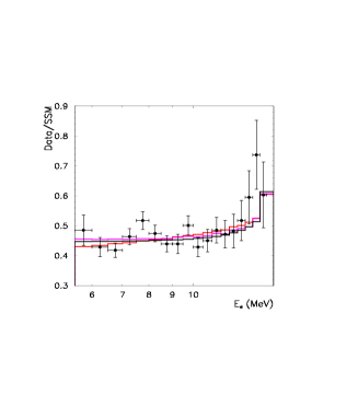
Figure 7: Expected normalized recoil electron energy spectra versus 708–day SK data, from [78].

Fig. 7 shows the expected normalized recoil electron energy spectrum compared with the most recent experimental data [6]. The solid line represents the prediction for the best–fit SMA solution with free ${}^{8}B$ and $hep$ normalizations (0.69 and 12 respectively), while the dotted line gives the corresponding prediction for the best–fit LMA solution (1.15 and 34 respectively). Finally, the dashed line represents the prediction for the best no-oscillation scheme with free ${}^{8}B$ and $hep$ normalizations (0.44 and 14, respectively). Clearly the spectra with enhanced $hep$ neutrinos provide better fits to the data. However Fiorentini et al [79] have argued that the required $hep$ amount is too large to accept on theoretical grounds. We look forward to the improvement of the situation in the next round of data. The increasing rôle played rate-independent observables such as the spectrum, as well as seasonal and day-night asymmetries, marks a turning point in solar neutrino research, which will eventually select the mechanism responsible for the explanation of the solar neutrino problem.

The required solar neutrino parameters are determined through a $\chi^{2}$ fit of the experimental data. In Fig. (8) we show the allowed regions in $\Delta m^{2}$ and $\sin^{2}\theta$ from the measurements of the total event rates at the Chlorine, Gallium and Super–Kamiokande (708-day data sample) combined with the zenith angle distribution observed in Super–Kamiokande, the recoil energy spectrum and the seasonal dependence of the event rates, for active-active oscillations (a) and active-sterile oscillations (b) . The darker (lighter) areas indicate 90% (99 %)CL regions. The best–fit points in each region are indicated by a star. The analysis uses free ${}^{8}B$ and $hep$ normalizations [78]

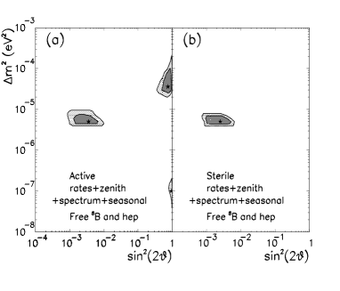
Figure 8: Solar neutrino parameters for 2-flavour MSW neutrino conversions with 708–day SK data sample and enhanced $hep$ flux  [78]

One notices from the analysis that rate-independent observables, such as the electron recoil energy spectrum and the day-night asymmetry (zenith angle distribution), are playing an increasing rôle in ruling out large regions of parameters [78]. Another example of an observable which has been neglected in most analyses of the MSW effect and which could be sizeable for the large mixing angle (LMA) region is the seasonal dependence in the solar neutrino flux which would result from the regeneration effect at the Earth and which has been discussed in ref. [80]. This should play a more significant rôle in future investigations.

A theoretical issue which has raised some interest recently is the study of the possible effect of random fluctuations in the solar matter density [81, 82, 83]. The possible existence of noise fluctuations at a few percent level is not excluded by present helioseismology studies.

Figure 9: Solar neutrino survival probability in a noisy Sun, from ref. [82]

In Fig. (9) we show averaged solar neutrino survival probability as a function of $E/\Delta m^{2}$, for $\sin^{2}2\theta=0.01$. This figure was obtained via a numerical integration of the MSW evolution equation in the presence of noise, using the density profile in the Sun from BP95 in ref. [67], and assuming that the correlation length $L_{0}$ (which corresponds to the scale of the fluctuation) is $L_{0}=0.1\lambda_{m}$, where $\lambda_{m}$ is the neutrino oscillation length in matter. An important assumption in the analysis is that $l_{free}\ll L_{0}\ll\lambda_{m}$, where $l_{free}\sim 10$ cm is the mean free path of the electrons in the solar medium. The fluctuations may strongly affect the ⁷Be neutrino component of the solar neutrino spectrum so that the Borexino experiment should provide an ideal test, if sufficiently small errors can be achieved. The potential of Borexino in probing the level of solar matter density fluctuations provides an additional motivation for the experiment [84].

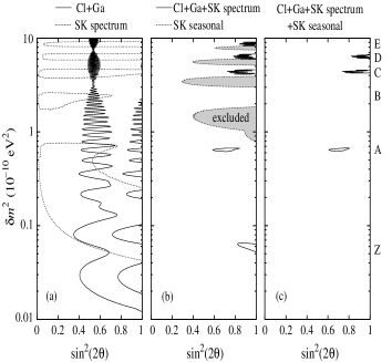
Figure 10: Vacuum oscillation parameters, from ref. [85]

The most popular alternative solution to the solar neutrino problem is the vacuum oscillation solution [70] which clearly requires large neutrino mixing and to adjust the oscillation length so as to coincide roughly with the Earth-Sun distance. This solution fits well with some theoretical models [72]. Fig. 10 shows the regions of just-so oscillation parameters at the 95 % CL obtained in a recent fit of the data, including both the rates, the recoil energy spectrum and seasonal effects, which are expected in this scenario  [86] and could potentially help in discriminating it from the MSW scenario.

3.2 Atmospheric Neutrinos

There has been a long-standing discrepancy between the predicted and measured $\nu_{\mu}$ /$\nu_{e}$ ratio [2] of the fluxes of atmospheric neutrinos [87]. The anomaly was found both in water Cerenkov experiments, Kamiokande, Super-Kamiokande and IMB [4], as well as in the iron calorimeter Soudan2 experiment. Negative experiments, such as Frejus and Nusex have much larger errors.

Although individual $\nu_{\mu}$ or $\nu_{e}$ fluxes are only known to within $30\%$ accuracy, the $\nu_{\mu}$ $/\nu_{e}$ ratio is known to $5\%$. The most important feature of the atmospheric neutrino 535-day  data sample [3] is that it exhibits a zenith-angle-dependent deficit of muon neutrinos which is inconsistent with theoretical expectations. For recent analyses see ref. [88, 89]. Experimental biases and uncertainties in the prediction of neutrino fluxes and cross sections are unable to explain the data.

Fig. 11 shows the measured zenith angle distribution of electron-like and muon-like sub-GeV and multi-GeV events, as well as the one predicted in the absence of oscillation. It also gives the expected distribution in various neutrino oscillation schemes.

Figure 11: Expected zenith angle distributions for SK electron and muon-like sub-GeV and multi-GeV events in the SM (no-oscillation) and for the best-fit points of the various oscillation channels, from ref. [88].

The thick-solid histogram is the theoretically expected distribution in the absence of oscillation, while the predictions for the best-fit points of the various oscillation channels is indicated as follows: for $\nu_{\mu}\to\nu_{s}$ (solid line), $\nu_{\mu}\to\nu_{e}$ (dashed line) and $\nu_{\mu}\to\nu_{\tau}$ (dotted line). The error displayed in the experimental points is only statistical. The analysis used the latest improved calculations of the atmospheric neutrino fluxes as a function of zenith angle, including the muon polarization effect and took into account a variable neutrino production point [90].

Clearly the data are not reproduced by the no-oscillation hypothesis. The most popular way to account for this anomaly is in terms of neutrino oscillations. In Fig. (12) I show the allowed parameters obtained in a global fit of the sub-GeV and multi-GeV (vertex-contained) atmospheric neutrino data [88] including the 535 day SK data, as well as all other experiments combined at 90 (thick solid line) and 99 % CL (thin solid line) for each oscillation channel considered.

Figure 12: Allowed atmospheric oscillation parameters for all experiments including the 535-day SK data, combined at 90 (thick solid line) and 99 % CL (thin solid line) for all possible oscillation channels, from ref. [88]. In each case the best-fit point is denoted by a star and always corresponds to maximal mixing, a feature which is well-reproduced by the theoretical predictions of the models proposed in ref. [18, 19]. The sensitivity of the present accelerator and reactor experiments as well as the expectations of upcoming long-baseline experiments is also displayed.

The two lower panels Fig. (12) differ in the sign of the $\Delta m^{2}$ which was assumed in the analysis of the matter effects in the Earth for the $\nu_{\mu}\to\nu_{s}$ oscillations. Though $\nu_{\mu}\to\nu_{\tau}$ oscillations give a slightly better fit than $\nu_{\mu}\to\nu_{s}$ oscillations, at present the atmospheric neutrino data cannot distinguish between these channels. It is well-known that the neutral-to-charged current ratios are important observables in neutrino oscillation phenomenology, which are especially sensitive to the existence of singlet neutrinos, light or heavy [24]. The atmospheric neutrinos produce isolated neutral pions ($\pi^{0}$-events) mainly in neutral current interactions. One may therefore study the ratios of $\pi^{0}$-events and the events induced mainly by the charged currents, as recently advocated in ref. [91]. This minimizes uncertainties related to the original atmospheric neutrino fluxes. In fact the Super-Kamiokande collaboration has estimated the double ratio of $\pi^{0}$ over e-like events in their sample [3] and found $R=0.93\pm 0.07\pm 0.19$. This is consistent both with $\nu_{\mu}$ to $\nu_{\tau}$ or $\nu_{\mu}$ to $\nu_{s}$ channels, with a slight preference for the former. The situation should improve in the future. We also display in Fig. (12) the sensitivity of present accelerator and reactor experiments, as well as that expected at future long-baseline (LBL) experiments. The first point to note is that the Chooz reactor [92] data excludes the region indicated for the $\nu_{\mu}\to\nu_{e}$ channel when all experiments are combined at 90% CL.

From the upper-left panel in Fig. (12) one sees that the regions of $\nu_{\mu}\to\nu_{\tau}$ oscillation parameters obtained from the atmospheric neutrino data analysis cannot be fully tested by the LBL experiments, as presently designed. One might expect that, due to the upward shift of the $\Delta m^{2}$ indicated by the fit for the sterile case (due to the effects of matter in the Earth) it would be possible to completely cover the corresponding region of oscillation parameters. Although this is the case for the MINOS disappearance test, in general most of the LBL experiments can not completely probe the region of oscillation parameters indicated by the $\nu_{\mu}\to\nu_{s}$ atmospheric neutrino analysis, irrespective of the sign of $\Delta m^{2}$ assumed. For a discussion of the various potential tests that can be performed at the future LBL experiments in order to unravel the presence of oscillations into sterile channels see ref. [93].

However appealing it may be, the neutrino oscillation interpretation of the atmospheric neutrino anomaly is at the moment by no means unique. Indeed, the anomaly can be well accounted for in terms of flavour changing neutrino interactions, with no need for neutrino mass or mixing [16]. Investigations involving upward through going muons by Superkamiokande [94] as well as other experiments will play an important rôle in discriminating between oscillations and alternative mechanisms to explain the sub and multi-GeV atmospheric neutrino data [95].

3.3 Other Hints

3.3.1 LSND

The Los Alamos Meson Physics Facility looked for $\bar{\nu}_{\mu}\to\bar{\nu}_{e}$ oscillations using $\bar{\nu}_{\mu}$ from $\mu^{+}$ decay at rest [8]. The $\bar{\nu}_{e}$’s are detected via the reaction $\bar{\nu}_{e}\,p\to e^{+}\,n$, correlated with a $\gamma$ from $np\to d\gamma$ ($2.2\,{\rm MeV}$). The results indicate $\bar{\nu}_{\mu}\to\bar{\nu}_{e}$ oscillations, with an oscillation probability of ($0.31^{+0.11}_{-0.10}\pm 0.05$)%, leading to the oscillation parameters shown in Fig. (13). The shaded regions are the favoured likelihood regions given in ref. [8]. The curves show the 90 % and 99 % likelihood allowed ranges from LSND, and the limits from BNL776, KARMEN1, Bugey, CCFR, and NOMAD.

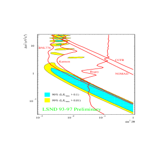
Figure 13: Allowed LSND oscillation parameters versus competing experiments [96]

A search for $\nu_{\mu}$ $\to$ $\nu_{e}$ oscillations has also been conducted by the LSND collaboration. Using $\nu_{\mu}$ from $\pi^{+}$ decay in flight, the $\nu_{e}$ appearance is detected via the charged-current reaction $C(\hbox{$\nu_{e}$ },e^{-})X$. Two independent analyses are consistent with the above signature, after taking into account the events expected from the $\nu_{e}$ contamination in the beam and the beam-off background. If interpreted as an oscillation signal, the observed oscillation probability of $2.6\pm 1.0\pm 0.5\times 10^{-3}$, consistent with the evidence for oscillation in the $\bar{\nu}_{\mu}$ $\to$ $\bar{\nu}_{e}$ channel described above. Fig. 14 compares the LSND region with the expected sensitivity from MiniBooNE, which was recently approved to run at Fermilab [96, 9].

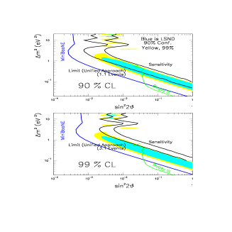
Figure 14: Expected sensitivity of the proposed MiniBooNE experiment [96]

A possible confirmation of the LSND anomaly would be a discovery of far-reaching implications.

3.3.2 Dark Matter

Galaxies as well as the large scale structure in the Universe should arise from the gravitational collapse of fluctuations in the expanding universe. They are sensitive to the nature of the cosmological dark matter. The data on cosmic background temperature anisotropies on large scales performed by the COBE satellite [97] combined with cluster-cluster correlation data e.g. from IRAS [98] can not be reconciled with the simplest COBE-normalized $\Omega_{m}=1$ cold dark matter (CDM) model, since it leads to too much power on small scales. Adding to CDM neutrinos with mass of few eV (a scale similar to the one indicated by the LSND experiment [8]) corresponding to $\Omega_{\nu}\approx 0.2$, results in an improved fit to data on the nearby galaxy and cluster distribution [99]. The resulting Cold + Hot Dark Matter (CHDM) cosmological model is the most successful $\Omega_{m}=1$ model for structure formation, preferred by inflation. However, other recent data have begun to indicate a lower value for $\Omega_{m}$, thus weakening the cosmological evidence favouring neutrino mass of a few eV in flat models with cosmological constant $\Omega_{\Lambda}=1-\Omega_{m}$ [99]. Future sky maps of the cosmic microwave background radiation (CMBR) with high precision at the MAP and PLANCK missions should bring more light into the nature of the dark matter and the possible rôle of neutrinos [100]. Another possibility is to consider unstable dark matter scenarios [101]. For example, an MeV range tau neutrino may provide a viable unstable dark matter scenario [102] if the $\nu_{\tau}$ decays before the matter dominance epoch. Its decay products would add energy to the radiation, thereby delaying the time at which the matter and radiation contributions to the energy density of the universe become equal. Such delay would allow one to reduce the density fluctuations on the smaller scales purely within the standard cold dark matter scenario. Upcoming MAP and PLANCK missions may place limits on neutrino stability [103] and rule out such schemes.

3.3.3 Pulsar Velocities

One of the most challenging problems in modern astrophysics is to find a consistent explanation for the high velocity of pulsars. Observations [104] show that these velocities range from zero up to 900 km/s with a mean value of $450\pm 50$ km/s. An attractive possibility is that pulsar motion arises from an asymmetric neutrino emission during the supernova explosion. In fact, neutrinos carry more than $99\%$ of the new-born proto-neutron star’s gravitational binding energy so that even a $1\%$ asymmetry in the neutrino emission could generate the observed pulsar velocities. This could in principle arise from the interplay between the parity violation present in weak interactions with the strong magnetic fields which are expected during a SN explosion [105, 106]. However, it has recently been noted [107] that no asymmetry in neutrino emission can be generated in thermal equilibrium, even in the presence of parity violation. This suggests that an alternative mechanism is at work. Several neutrino conversion mechanisms in matter have been invoked as a possible engine for powering pulsar motion. They all rely on the polarization [108] of the SN medium induced by the strong magnetic fields $10^{15}$ Gauss present during a SN explosion. This would affect neutrino propagation properties giving rise to an angular dependence of the matter-induced neutrino potentials. This would lead in turn to a deformation of the ”neutrino-sphere” for, say, tau neutrinos and thus to an anisotropic neutrino emission. As a consequence, in the presence of non-vanishing $\nu_{\tau}$ mass and mixing the resonance sphere for the $\nu_{e}-\nu_{\tau}$ conversions is distorted. If the resonance surface lies between the $\nu_{\tau}$ and $\nu_{e}$ neutrino spheres, such a distortion would induce a temperature anisotropy in the flux of the escaping tau-neutrinos produced by the conversions, hence a recoil kick of the proto-neutron star. This mechanism was realized in ref. [109] invoking MSW conversions [34] with $m_{\nu_{\tau}}$ $\;>$$\sim\;$ 100 eV or so, assuming a negligible $\nu_{e}$ mass. This is necessary in order for the resonance surface to be located between the two neutrino-spheres. It should be noted, however, that such requirement is at odds with cosmological bounds on neutrinos masses unless the $\tau$-neutrino is unstable. On the other hand in ref. [110] a realization was proposed in the resonant spin-flavour precession scheme (RSFP) [73]. The magnetic field would not only affect the medium properties, but would also induce the spin-flavour precession through its coupling to the neutrino transition magnetic moment [75].

Perhaps the simplest suggestion was proposed in ref. [36] where the required pulsar velocities would arise from anisotropic neutrino emission induced by resonant conversions of massless neutrinos (hence no magnetic moment).

Raffelt and Janka [111] have argued, however, that the asymmetric neutrino emission effect was overestimated, since the temperature variation over the deformed neutrino-sphere is not an adequate measure for the anisotropy of the neutrino emission. This would invalidate all neutrino conversion mechanisms, leaving the pulsar velocity problem without any known viable solution. One potential way out would invoke conversions into sterile neutrinos, since the conversions would take place deeper in the star. However, it is too early to tell whether or not it works [112].

4 Fitting the Puzzles Together

Physics beyond the Standard Model is required in order to explain solar and atmospheric neutrino data. While neutrino oscillations provide an excellent fit, alternative mechanisms are still viable. Thus it is still too early to tell for sure whether neutrino masses and angles are really being determined experimentally. Here we assume the standard neutrino oscillation interpretation of the data. While it can easily be accommodated in theories of neutrino mass, in general the angles involved are not predicted, in particular the maximal mixing indicated by the atmospheric data. It is suggestive to consider a theory with bi-maximal mixing of neutrinos [71] if the solar neutrino data are explained in terms of the just-so solution. This is not easy to reconcile in a predictive quark-lepton unification scheme that relates lepton and quark mixing angles, since the latter are known to be small. For recent attempts to reconcile solar and atmospheric data in unified models with specific texture anzatze, see ref. [25, 113]. The story gets more complicated if one wishes to account also for the LSND anomaly and for the hot dark matter [18, 19, 20]. As we have seen the atmospheric neutrino data requires $\Delta m^{2}_{atm}$ which is much larger than the scale $\Delta{m^{2}}_{\odot}$ which is indicated by the solar neutrino data. This implies that with just the three known neutrinos there is no room, unless some of the experimental data are discarded.

4.1 Almost Degenerate Neutrinos

The only possibility to fit solar, atmospheric and HDM scales in a world with just the three known neutrinos is if all of them have nearly the same mass [20], of about $\sim$ 1.5 eV or so in order to provide the right amount of HDM [99] (all three active neutrinos contribute to HDM). This can be arranged in the unification approach discussed in sec. 2 using the $M_{L}$ term present in general in seesaw models. With this in mind one can construct, e.g. unified $SO(10)$ seesaw models where all neutrinos lie at the above HDM mass scale ($\sim$ 1.5 eV), due to a suitable horizontal symmetry, while the parameters $\Delta{m^{2}}_{\odot}$ & $\Delta{m^{2}}_{atm}$ appear as symmetry breaking effects. An interesting fact is that the ratio $\Delta{m^{2}}_{\odot}\>/\>\Delta{m^{2}}_{atm}$ appears as ${m_{c}}^{2}/{m_{t}}^{2}$ [26]. There is no room in this case to accommodate the LSND anomaly. To what extent this solution is theoretically natural has been discussed recently in ref. [114].

4.2 Four-Neutrino Models

The simplest way to incorporate the LSND scale is to invoke a fourth neutrino. It must be $SU(2)\otimes U(1)$ singlet ensuring that it does not affect the invisible Z decay width, well-measured at LEP. The sterile neutrino $\nu_{s}$ must also be light enough in order to participate in the oscillations together with the three active neutrinos. The theoretical challenges we have are:

• to understand what keeps the sterile neutrino light, since the $SU(2)\otimes U(1)$ gauge symmetry would allow it to have a large bare mass

• to account for the maximal neutrino mixing indicated by the atmospheric data, and possibly by the solar

• to account from first principles for the scales $\Delta m^{2}_{atm}$, $\Delta{m^{2}}_{\odot}$ and $\Delta m^{2}_{LSND/HDM}$

With this in mind we have formulated the simplest maximally symmetric schemes, denoted as $(e\tau)(\mu~{}s)$ [18] and $(es)(\mu\tau)$  [19], respectively. One should realize that a given scheme (mainly the structure of the leptonic charged current) may be realized in more than one theoretical model. For example, an alternative to the model in  [19] was suggested in ref. [20]. There have been many attempts to derive the above phenomenological scenarios from different theoretical assumptions, as has been discussed here [115, 116].

Although many of the phenomenological features arise also in other models, here I concentrate the discussion mainly on the theories developed in ref. [18, 19]. These are characterized by a very symmetric mass spectrum in which there are two ultra-light neutrinos at the solar neutrino scale and two maximally mixed almost degenerate eV-mass neutrinos (LSND/HDM scale), split by the atmospheric neutrino scale [18, 19]. The HDM problem requires the heaviest neutrinos at about 2 eV mass [117]. These scales are generated radiatively due to the additional Higgs bosons which are postulated, as follows: $\Delta m^{2}_{LSND/HDM}$ arises at one-loop, while $\Delta m^{2}_{atm}$ and $\Delta{m^{2}}_{\odot}$ are two-loop effects. Since these models pre-dated the LSND results, they naturally focussed on accounting for the HDM problem, rather than LSND. However, in the meantime the evidence for hot dark matter has weakened, whereas LSND came into play. In contrast to the HDM problem, the LSND anomaly, if confirmed, would be a more convincing indication for the existence of a fourth light neutrino species, considering that the HDM may be accounted for in a three neutrino degenerate scenario.

The models in  [18, 19] are based only on weak-scale physics. They explain the lightness of the sterile neutrino, the large lepton mixing required by the atmospheric neutrino data, as well as the generation of the mass splittings responsible for solar and atmospheric neutrino conversions as natural consequences of the underlying lepton-number-like symmetry and its breaking. They are minimal in the sense that they add a single $SU(2)\otimes U(1)$ singlet lepton to the SM. Before breaking the symmetry the heaviest neutrinos are exactly degenerate, while the other two are still massless [118]. After the global U(1) lepton symmetry breaks the heavier neutrinos split and the lighter ones get mass. The models differ according to whether the $\nu_{s}$ lies at the dark matter scale or at the solar neutrino scale. In the $(e\tau)(\mu~{}s)$ scheme the $\nu_{s}$ lies at the LSND/HDM scale, as illustrated in Fig. (15)

Figure 15: $(e\tau)(\mu~{}s)$ scheme: $\nu_{e}$ - $\nu_{\tau}$ conversions explain the solar neutrino data and $\nu_{\mu}$ - $\nu_{s}$ oscillations account for the atmospheric deficit, ref. [18].

while in the alternative $(es)(\mu\tau)$ model, $\nu_{s}$ is at the solar neutrino scale as shown in Fig. (16) [19].

Figure 16: $(es)(\mu\tau)$ scheme: $\nu_{e}$ - $\nu_{s}$ conversions explain the solar neutrino data and $\nu_{\mu}$ - $\nu_{\tau}$ oscillations account for the atmospheric deficit, ref. [19].

In the $(e\tau)(\mu~{}s)$ case the atmospheric neutrino puzzle is explained by $\nu_{\mu}$ to $\nu_{s}$ oscillations, while in $(es)(\mu\tau)$ it is due to $\nu_{\mu}$ to $\nu_{\tau}$ oscillations. Correspondingly, the deficit of solar neutrinos is explained in the first case by $\nu_{e}$ to $\nu_{\tau}$ conversions, while in the second the relevant channel is $\nu_{e}$ to $\nu_{s}$.

The presence of additional weakly interacting light particles, such as our light sterile neutrino, is constrained by BBN since the $\nu_{s}$ would enter into equilibrium with the active neutrinos in the early Universe (and therefore would contribute to $N_{\nu}^{max}$) via neutrino oscillations [119], unless $\Delta m^{2}sin^{4}2\theta\raise 1.29167pt\hbox{$\;<$\kern-7.5pt\raise-4.73611pt\hbox{$\sim\;$}}3\times 10^{-6}~{}~{}eV^{2}$ Here $\Delta m^{2}$ denotes the mass-square difference of the active and sterile species and $\theta$ is the vacuum mixing angle. However, systematic uncertainties in the BBN bounds still caution us not to take them too literally. For example, it has been argued that present observations of primordial Helium and deuterium abundances may allow up to $N_{\nu}=4.5$ neutrino species if the baryon to photon ratio is small [58]. Adopting this as a limit, clearly both models described above are consistent. Should the BBN constraints get tighter [59] e.g. $N_{\nu}^{max}<3.5$ they could rule out the $(e\tau)(\mu~{}s)$ model, and leave out only the competing scheme as a viable alternative. However the possible rôle of a primordial lepton asymmetry might invalidate this conclusion, for recent work on this see ref. [120].

The two models would be distinguishable both at future solar as well as atmospheric neutrino data. For example they may be tested in the SNO experiment [121] once they measure the solar neutrino flux ($\Phi^{NC}_{\nu}$) in their neutral current data and compare it with the corresponding CC value ($\Phi^{CC}_{\nu}$). If the solar neutrinos convert to active neutrinos, as in the $(e\tau)(\mu~{}s)$ model, then one expects $\Phi^{CC}_{\nu}/\Phi^{NC}_{\nu}$ around 0.5, whereas in the $(es)(\mu\tau)$ scheme ($\nu_{e}$ conversion to $\nu_{s}$ ), the above ratio would be nearly $\simeq 1$. Looking at pion production via the neutral current reaction $\nu_{\tau}+N\to\nu_{\tau}+\pi^{0}+N$ in atmospheric data might also help in distinguishing between these two possibilities [91], since this reaction is absent in the case of sterile neutrinos, but would exist in the $(es)(\mu\tau)$ scheme.

If light sterile neutrinos indeed exist one can show that they might contribute to a cosmic hot dark matter component and to an increased radiation content at the epoch of matter-radiation equality. These effects leave their imprint in sky maps of the cosmic microwave background radiation (CMBR) and may thus be detectable with the very high precision measurements expected at the upcoming MAP and PLANCK missions as noted recently in ref. [100].

4.3 MeV Tau Neutrino

In ref. [122] a model was presented where an unstable MeV Majorana tau neutrino naturally reconciles the cosmological observations of large and small-scale density fluctuations with the cold dark matter picture. The model assumes the spontaneous violation of a global lepton number symmetry at the weak scale. The breaking of this symmetry generates the cosmologically required decay of the $\nu_{\tau}$ with lifetime $\tau_{\nu_{\tau}}\sim 10^{2}-10^{4}$ sec, as well as the masses and oscillations of the three light neutrinos $\nu_{e}$ , $\nu_{\mu}$ and $\nu_{s}$ which may account for the present solar and atmospheric data, though this will have to be checked. One can also verify that the BBN constraints can be satisfied.

5 In conclusion

The confirmation of an angle-dependent atmospheric neutrino deficit provides, together with the solar neutrino data, a strong evidence for physics beyond the Standard Model. Small neutrino masses provide the simplest, but not unique, explanation of the data. If the LSND result stands the test of time, this would be a puzzling indication for the existence of a light sterile neutrino. The two most attractive schemes to reconcile underground observations with LSND invoke either $\nu_{e}$ - $\nu_{\tau}$ conversions to explain the solar data, with $\nu_{\mu}$ - $\nu_{s}$ oscillations accounting for the atmospheric deficit, or the opposite. These two basic schemes have distinct implications at future solar & atmospheric neutrino experiments. SNO and Super-Kamiokande have the potential to distinguish them due to their neutral current sensitivity.

Allowing for alternative explanations of the data from underground experiments one can still live with massless non-standard neutrinos or even very heavy neutrinos, which may naturally arise in many models. Although cosmological bounds are a fundamental tool to restrict neutrino masses, in many theories heavy neutrinos will either decay or annihilate very fast, thereby loosening the cosmological bounds. From this point of view, neutrinos can have any mass presently allowed by laboratory experiments, and it is therefore important to search for manifestations of heavy neutrinos at the laboratory in an unbiased way.

Last but not least, though most of the recent excitement comes from underground experiments, one should note that models of neutrino mass may lead to a plethora of new signatures which may be accessible also at accelerators, thus illustrating the complementarity between the two approaches in unravelling the properties of neutrinos and probing for signals beyond the Standard Model [47].

I am grateful to the Organizers for the kind hospitality at Corfu. This work was supported by DGICYT grant PB95-1077 and by the EEC under the TMR contract ERBFMRX-CT96-0090.

References

- [1] Invited talks by Lande, Gavrin, Kirsten, and Suzuki at Neutrino 98, Takayama, Japan
- [2] NUSEX Collaboration, M. Aglietta et al., Europhys. Lett. 8, 611 (1989); Fréjus Collaboration, Ch. Berger et al., Phys. Lett. B227, 489 (1989); IMB Collaboration, D. Casper et al., Phys. Rev. Lett. 66, 2561 (1991); R. Becker-Szendy et al., Phys. Rev. D46, 3720 (1992); Kamiokande Collaboration, H. S. Hirata et al., Phys. Lett. B205, 416 (1988) and Phys. Lett. B280, 146 (1992); Kamiokande Collaboration, Y. Fukuda et al., Phys. Lett. B335, 237 (1994); Soudan Collaboration, W. W. M Allison et al., Phys. Lett. B391, 491 (1997).
- [3] T. Kajita, Invited talk at Neutrino 98, Takayama, Japan
- [4] C. Yanagisawa, talk at the International Workshop on Physics Beyond The Standard Model: from Theory to Experiment, Valencia, (World Scientific, 1998, ISBN 981-02-3638-7), http://flamenco.uv.es//val97.html
- [5] Y. Suzuki, Invited talk at Neutrino 98, Takayama, Japan
- [6] M.B. Smy, “Solar neutrinos with SuperKamiokande,” hep-ex/9903034.
- [7] K. Inoue, talk at Neutrino Telescopes Workshop, Venice, Feb. 1999.
- [8] C. Athanassopoulos, [LSND Collaboration], Phys. Rev. Lett. 75 (1995) 2650; Phys. Rev. Lett. 77 (1996) 3082 ; C. Athanassopoulos et al, Phys. Rev. Lett. 81, 1774 (1998)
- [9] W.C. Louis [LSND Collaboration], Prog. Part. Nucl. Phys. 40, 151 (1998).
- [10] For reviews see J. W. F. Valle, Gauge Theories and the Physics of Neutrino Mass, Prog. Part. Nucl. Phys. 26 (1991) 91-171
- [11] J. Bernabeu, A. Santamaria, J. Vidal, A. Mendez, J. W. F. Valle, Phys. Lett. B187 (1987) 303; J. G. Korner, A. Pilaftsis, K. Schilcher, Phys. Lett. B300 (1993) 381
- [12] M. C. Gonzalez-Garcia, J. W. F. Valle, Mod. Phys. Lett. A7 (1992) 477; erratum Mod. Phys. Lett. A9 (1994) 2569; A. Ilakovac, A. Pilaftsis, Nucl. Phys. B437 (1995) 491; A. Pilaftsis, Mod. Phys. Lett. A9 (1994) 3595
- [13] D. Wyler, L. Wolfenstein, Nucl. Phys. B218 (1983) 205
- [14] R. Mohapatra, J. W. F. Valle, Phys. Rev. D34 (1986) 1642; J. W. F. Valle, Nucl. Phys. B (Proc. Suppl.) B11 (1989) 118-177
- [15] L.J. Hall, V.A. Kostelecky and S. Raby, Nucl. Phys. B267, 415 (1986).
- [16] M.C. Gonzalez-Garcia et al., Phys. Rev. Lett. 82 (1999) 3202 hep-ph/9809531.
- [17] J. Schechter and J.W. Valle, Phys. Rev. D25, 2951 (1982); for reviews see A. Morales, “Review on double beta decay experiments and comparison with theory,” hep-ph/9809540; B. Kayser, “Neutrino mass physics,” 28th Rencontres de Moriond: Electroweak Interactions and Unified Theories, Les Arcs, France, Mar 1993.
- [18] J. T. Peltoniemi, D. Tommasini, and J W F Valle, Phys. Lett. B298 (1993) 383
- [19] J. T. Peltoniemi, and J W F Valle, Nucl. Phys. B406 (1993) 409
- [20] D.O. Caldwell and R.N. Mohapatra, Phys. Rev. D48 (1993) 3259
- [21] See, e.g. R. N. Mohapatra and G. Senjanovic, Phys. Rev. D23 (1981) 165.
- [22] J.C. Pati, A. Salam. Phys. Rev. D8 (1973) 1240
- [23] M Gell-Mann, P Ramond, R. Slansky, in Supergravity, ed. P.van Niewenhuizen and D. Freedman (North Holland, 1979); T. Yanagida, in KEK lectures, ed. O. Sawada and A. Sugamoto (KEK, 1979); R. N. Mohapatra and G. Senjanovic, Phys. Rev. Lett. 44 912 (1980).
- [24] J. Schechter and J. W. F. Valle, Phys. Rev. D22 (1980) 2227
- [25] S. Lola and J.D. Vergados, Prog. Part. Nucl. Phys. 40, 71 (1998); G. Altarelli and F. Feruglio, Phys. Lett. B439, 112 (1998) hep-ph/9807353.
- [26] A. Ioannissyan, J. W. F. Valle, Phys. Lett. B332 (1994) 93-99; B. Bamert, C.P. Burgess, Phys. Lett. B329 (1994) 289; D. Caldwell and R. N. Mohapatra, Phys. Rev. D50 (1994) 3477; D. G. Lee and R. N. Mohapatra, Phys. Lett. B329 (1994) 463; A. S. Joshipura, Zeit. fur Physik C64 (1994) 31
- [27] M. C. Gonzalez-Garcia, J. W. F. Valle, Phys. Lett. B216 (1989) 360.
- [28] M. Dittmar, M. C. Gonzalez-Garcia, A. Santamaria, J. W. F. Valle, Nucl. Phys. B332 (1990) 1; M. C. Gonzalez-Garcia, A. Santamaria, J. W. F. Valle, ibid. B342 (1990) 108; J . Gluza, J. Maalampi, M. Raidal, M. Zralek, Phys. Lett. B407 (1997) 45; J. Gluza, M. Zralek; Phys. Rev. D55 (1997) 7030
- [29] G. C. Branco, M. N. Rebelo, J. W. F. Valle, Phys. Lett. B225 (1989) 385; N. Rius, J. W. F. Valle, Phys. Lett. B246 (1990) 249
- [30] M. Dittmar, J. W. F. Valle, contribution to the High Luminosity at LEP working group, yellow report CERN-91/02, p. 98-103
- [31] R. Alemany et. al. hep-ph/9307252, published in ECFA/93-151, ed. R. Aleksan, A. Ali, p. 191-211
- [32] Opal collaboration, Phys. Lett. B254 (1991) 293 and Zeit. fur Physik C67 (1995) 365; L3 collaboration, Phys. Rep. 236 (1993) 1-146; Phys. Lett. B316 (1993) 427, Delphi collaboration, Phys. Lett. B359 (1995) 411.
- [33] J. W. F. Valle, Phys. Lett. B199 (1987) 432
- [34] A.Y. Smirnov and S.P. Mikheev, “Neutrino Oscillations In Matter With Varying Density,” In *Tignes 1986, Proceedings, ’86 massive neutrinos* 355-372; L. Wolfenstein, Phys. Rev. D20 (1979) 2634.
- [35] H. Nunokawa, Y.Z. Qian, A. Rossi, J. W. F. Valle, Phys. Rev. D54 (1996) 4356-4363, hep-ph/9605301
- [36] D. Grasso, H. Nunokawa and J. W. F. Valle, Phys. Rev. Lett. 81, 2412 (1998), astro-ph/9803002.
- [37] A. Zee, Phys. Lett. B93 (1980) 389
- [38] K. S. Babu, Phys. Lett. B203 (1988) 132
- [39] J. T. Peltoniemi, and J. W. F. Valle, Phys. Lett. B304 (1993) 147
-
[40]
M.A. Díaz, J.C. Romão, and J. W. F. Valle,
Nucl. Phys. B524 23-40 (1998),
hep-ph/9706315. - [41] F. Vissani and A. Yu. Smirnov, Nucl. Phys. B460, 37-56 (1996); R. Hempfling, Nucl. Phys. B478, 3 (1996), and hep-ph/9702412; H.P. Nilles and N. Polonsky, Nucl. Phys. B484, 33 (1997); B. de Carlos, P.L. White, Phys.Rev. D55 4222-4239 (1997); E. Nardi, Phys. Rev. D55 (1997) 5772; S. Roy and B. Mukhopadhyaya, Phys. Rev. D55, 7020 (1997); A.S. Joshipura and M. Nowakowski, Phys. Rev. D 51, 2421 (1995); T. Banks, Y. Grossman, E. Nardi, and Y. Nir, Phys. Rev. D 52, 5319 (1995); F.M. Borzumati, Y. Grossman, E. Nardi, Y. Nir, Phys. Lett. B 384, 123 (1996); A. Faessler, S. Kovalenko and F. Simkovic, Phys. Rev. D58, 055004 (1998), hep-ph/9712535; M. Carena, S. Pokorski and C.E. Wagner, Phys. Lett. B430, 281 (1998) hep-ph/9801251; M.E. Gómez and K. Tamvakis, hep-ph/9801348.
- [42] M.A. Díaz, hep-ph/9711435, hep-ph/9712213; J.C. Romão, hep-ph/9712362 and J. W. F. Valle, hep-ph/9808292.
- [43] G.G. Ross, J. W. F. Valle. Phys. Lett. 151B 375 (1985); John Ellis, G. Gelmini, C. Jarlskog, G.G. Ross, J. W. F. Valle, Phys. Lett. 150B 142 (1985); A. Santamaria, J. W. F. Valle, Phys. Lett. 195B 423 (1987).
- [44] J. Schechter, J. W. F. Valle, Phys. Rev. D25 (1982) 774
- [45] See, e.g. A.D. Dolgov, S. Pastor, and J. W. F. Valle, Phys. Lett. B383 (1996) 193-198, hep-ph/9602233; S. Hannestad, J. Madsen, Phys. Rev. Lett. 76 (1996) 2848-2851, Erratum-ibid. 77 (1996) 5148; J.B. Rehm, G. G. Raffelt, A. Weiss Astron. & Astrophys. 327 (1997) 443-452, A. D. Dolgov, S. H. Hansen, D. V. Semikoz, Nucl. Phys. B524 (1998) 621-638
- [46] J. C. Romão, J. W. F. Valle, Nucl. Phys. B381 (1992) 87-108
- [47] For reviews see J. W. F. Valle, hep-ph/9712277 and hep-ph/9603307; see also M. A. Diaz, M. A. Garcia-Jareno, D. A. Restrepo, J. W. F. Valle, Nucl. Phys. B527 (1998) 44-60 and F. de Campos, O. J. P. Eboli, J. Rosiek, J. W. F. Valle, Phys. Rev.D55 (1997) 1316-1325, hep-ph 9601269.
- [48] Y. Chikashige, R. Mohapatra, R. Peccei, Phys. Rev. Lett. 45 (1980) 1926
- [49] E.K. Akhmedov, A.S. Joshipura, S. Ranfone and J. W. F. Valle, Nucl. Phys. B441 (1995) 61, hep-ph/9501248.
- [50] A. Joshipura and J. W. F. Valle, Nucl. Phys. B397 (1993) 105; J. C. Romao, F. de Campos, and J. W. F. Valle, Phys. Lett. B292 (1992) 329
- [51] R. Barbieri, J. Ellis & M. K. Gaillard, Phys. Lett. 90 B, 249 (1980); E. Akhmedov, Z. Berezhiani & G. Senjanović, Phys. Rev. Lett. 69, 3013 (1992).
- [52] V. Berezinskii, J. W. F. Valle Phys.Lett B318 360-366,1993, [hep-ph/9309214]
- [53] E. Kolb, M. Turner, The Early Universe, Addison-Wesley, 1990, and references therein
- [54] J. W. F. Valle, Phys. Lett. B131 (1983) 87; G. Gelmini, J. W. F. Valle, Phys. Lett. B142 (1984) 181; J. W. F. Valle, Phys. Lett. B159 (1985) 49; A. Joshipura, S. Rindani, Phys. Rev. D46 (1992) 3000
- [55] A. Masiero, J. W. F. Valle, Phys. Lett. B251 (1990) 273; J. C. Romao, C. A. Santos, and J. W. F. Valle, Phys. Lett. B288 (1992) 311; J.C. Romao, A. Ioannisian and J. W. F. Valle, Phys. Rev. D55, 427 (1997) hep-ph/9607401.
- [56] R.F. Carswell, MNRAS 268 (1994) L1; A. Songalia, L.L. Cowie, C. Hogan and M. Rugers, Nature 368 (1994) 599; D. Tytler and X.M. Fan, Bull. Am. Astr. Soc. 26 (1994) 1424; D. Tytler, talk at the Texas Symposium, December 1996.
- [57] N. Hata et al., Phys. Rev. Lett. 75 (1995) 3977; C.J. Copi, D.N. Schramm and M.S. Turner, Science 267 (1995) 192 and Phys. Rev. Lett. 75 (1995) 3981; K. A. Olive and G. Steigman, Phys. Lett. B354 (1995) 357-362;
- [58] S. Sarkar, Rep. Prog. Phys. 59, 1493 (1996); P. J. Kernan and S. Sarkar, Phys. Rev. D 54 (1996) R3681
- [59] G. Fiorentini, E. Lisi, S. Sarkar and F.L. Villante, “Quantifying uncertainties in primordial nucleosynthesis without Monte Carlo simulations,” Phys. Rev. D58, 063506 (1998); E. Lisi, S. Sarkar and F.L. Villante, Phys. Rev. D59, 123520 (1999)
- [60] A.D. Dolgov, S. Pastor, J.C. Romão and J. W. F. Valle, Nucl. Phys. B496 (1997) 24-40, hep-ph/9610507.
- [61] S. Hannestad, Phys. Rev. D57 (1998) 2213-2218; M. Kawasaki, K. Kohri, K. Sato, Phys. Lett. B430 (1998) 132-139; for a review see G. Steigman; in Cosmological Dark Matter, p. 55, World Scientific, 1994, ISBN 981-02-1879-6; A.D. Dolgov, S.H. Hansen, S. Pastor and D.V. Semikoz, Nucl. Phys. B548 (1999) 385-407
- [62] Y. Fukuda et al. [Super-Kamiokande Collaboration], “Measurement of the solar neutrino energy spectrum using neutrino electron scattering,” Phys. Rev. Lett. 82, 2430 (1999) hep-ex/9812011.
- [63] Y. Fukuda et al. [Super-Kamiokande Collaboration], “Constraints on neutrino oscillation parameters from the measurement of day night solar neutrino fluxes at SuperKamiokande,” Phys. Rev. Lett. 82, 1810 (1999) hep-ex/9812009.
- [64] Y. Fukuda et al. [Super-Kamiokande Collaboration], “Evidence for oscillation of atmospheric neutrinos,” Phys. Rev. Lett. 81, 1562 (1998) hep-ex/9807003; see also hep-ex/9803006 and hep-ex/9805006
- [65] J. N. Bahcall, S. Basu and M. H. Pinsonneault, Phys. Lett. B 433 (1998) 1.
- [66] J. N. Bahcall, astro-ph/9808162
- [67] (GONG) J. Christensen-Dalsgaard et al., GONG Collaboration, Science 272 (1996) 1286; (BP95) J. N. Bahcall and M. H. Pinsonneault, Rev. Mod. Phys. 67 (1995) 781; (KS94) A. Kovetz and G. Shaviv, Astrophys. J. 426 (1994) 787; (CDF94) V. Castellani, S. Degl’Innocenti, G. Fiorentini, L.M. Lissia and B. Ricci, Phys. Lett. B 324 (1994) 425; (JCD94) J. Christensen-Dalsgaard, Europhys. News 25 (1994) 71; (SSD94) X. Shi, D.N. Schramm and D.S.P. Dearborn, Phys. Rev. D 50 (1994) 2414; (DS96) A. Dar and G. Shaviv, Astrophys. J. 468 (1996) 933; (CDF93) V. Castellani, S. Degl’Innocenti and G. Fiorentini, Astron. Astrophys. 271 (1993) 601; (TCL93) S. Turck-Chièze and I. Lopes, Astrophys. J. 408 (1993) 347; (BPML93) G. Berthomieu, J. Provost, P. Morel and Y. Lebreton, Astron. Astrophys. 268 (1993) 775; (BP92) J.N. Bahcall and M.H. Pinsonneault, Rev. Mod. Phys. 64 (1992) 885; (SBF90) I.-J. Sackman, A.I. Boothroyd and W.A. Fowler, Astrophys. J. 360 (1990) 727; (BU88) J.N. Bahcall and R.K. Ulrich, Rev. Mod. Phys. 60 (1988) 297; (RVCD96) O. Richard, S. Vauclair, C. Charbonnel and W.A. Dziembowski, Astron. Astrophys. 312 (1996) 1000; (CDR97) F. Ciacio, S. Degl’Innocenti and B. Ricci, Astron. Astrophys. Suppl. Ser. 123 (1997) 449.
- [68] J.N. Bahcall, M.H. Pinsonneault, S. Basu and J. Christensen-Dalsgaard, Phys. Rev. Lett. 78 (1997) 171.
- [69] J. N. Bahcall, Phys. Lett. B338 (1994) 276; V. Castellani, et al Phys. Lett. B324 (1994) 245; N. Hata, S. Bludman, and P. Langacker, Phys. Rev. D49 (1994) 3622; V. Berezinsky, Comm. on Nucl. and Part. Phys. 21 (1994) 249
- [70] V. Barger, K. Whisnant and R.J. Phillips, Phys. Rev. D24, 538 (1981); S.L. Glashow and L.M. Krauss, Phys. Lett. 190B, 199 (1987); S.L. Glashow, P.J. Kernan and L.M. Krauss, Phys. Lett. B445, 412 (1999)
- [71] V. Barger, S. Pakvasa, T.J. Weiler and K. Whisnant, Phys. Lett. B437, 107 (1998), hep-ph/9806387; S. Davidson and S.F. King, Phys. Lett. B445, 191 (1998).
- [72] R.N. Mohapatra and J. W. F. Valle, Phys. Lett. 177B, 47 (1986).
- [73] E.Kh. Akhmedov, Phys. Lett. B213 (1988) 64-68; C. S. Lim and W. Marciano, Phys. Rev. D37 (1988) 1368
- [74] E.Kh. Akhmedov, The neutrino magnetic moment and time variations of the solar neutrino flux, hep-ph/9705451
- [75] J. Schechter, J. W. F. Valle, Phys. Rev. D24 1883, (1981), Err. ibid.D25 283, (1982).
- [76] P.I. Krastev and J.N. Bahcall, “FCNC solutions to the solar neutrino problem,” hep-ph/9703267.
- [77] J.N. Bahcall and P.I. Krastev, Phys. Lett. B436, 243 (1998); R. Escribano, J.M. Frere, A. Gevaert and D. Monderen, Phys. Lett. B444, 397 (1998).
- [78] M.C. Gonzalez-Garcia, P.C. de Holanda, C. Pena-Garay, and J. W. F. Valle, Status of the MSW Solutions of the Solar Neutrino Problem, hep-ph/9906469.
- [79] G. Fiorentini, V. Berezinsky, S. Degl’Innocenti and B. Ricci, “Bounds on hep neutrinos,” Phys. Lett. B444, 387 (1998) astro-ph/9810083.
- [80] P.C. de Holanda, C. Pena-Garay, M.C. Gonzalez-Garcia and J. W. F. Valle, “Seasonal dependence in the solar neutrino flux,” hep-ph/9903473; see also J.N. Bahcall, P.I. Krastev and A.Y. Smirnov, hep-ph/9905220.
- [81] A.B. Balantekin, J.M. Fetter and F.N. Loreti, Phys. Rev. D54 (1996) 3941-3951; F. N. Loreti and A. B. Balantekin, Phys. Rev. D50 (1994) 4762; F. N. Loreti et al., Phys. Rev. D52 (1996) 6664.
- [82] H. Nunokawa, A. Rossi, V. Semikoz, J. W. F. Valle, Nucl. Phys. B472 (1996) 495-517 [see also talk at Neutrino 96, hep-ph/9610526]
- [83] P. Bamert, C.P. Burgess and D. Michaud, Nucl. Phys. B513, 319 (1998); C.P. Burgess, hep-ph/9711425; C.P. Burgess and D. Michaud, Annals Phys. 256, 1 (1997) and hep-ph/9611368.
- [84] C. Arpesella at al., Proposal of the Borexino experiment (1991).
- [85] V. Barger, K. Whisnant, hep-ph/9903262
- [86] S.P. Mikheyev, A.Yu. Smirnov Phys.Lett. B429 (1998) 343-348; B. Faid, G. L. Fogli, E. Lisi, D. Montanino, hep-ph/9805293
- [87] T. K. Gaisser, F. Halzen and T. Stanev, Phys. Rep. 258, 174 (1995)
- [88] M. C. Gonzalez-Garcia, H. Nunokawa, O. L. G. Peres, T. Stanev, J. W. F. Valle, Phys. Rev. D58 (1998) 033004 [hep-ph 9801368]; for the 535 days data sample update, and the comparison of active and sterile channels see M.C. Gonzalez-Garcia, H. Nunokawa, O.L. Peres and J. W. F. Valle, Nucl. Phys. B543, 3 (1998), hep-ph/9807305.
- [89] R. Foot, R. R. Volkas, O. Yasuda, TMUP-HEL-9801; O. Yasuda, Phys. Rev. D58, 091301 (1998); G. L. Fogli, E. Lisi, A. Marrone, G. Scioscia, Phys. Rev. D59, 033001 (1999) ep-ph/9808205; E.Kh. Akhmedov, A.Dighe, P. Lipari and A.Yu. Smirnov, hep-ph/9808270.
- [90] V. Agrawal et al., Phys. Rev. D53, 1314 (1996); L. V. Volkova, Sov. J. Nucl. Phys. 31, 784 (1980); T. K. Gaisser and T. Stanev, Phys. Rev. D57 1977 (1998).
- [91] A. Smirnov and F. Vissani, Phys.Lett. B432 (1998) 376; J. G. Learned, S. Pakvasa and J. Stone, hep-ph/9805343; H. Murayama and L. Hall, hep-ph/9806218
- [92] M. Appollonio et al. Phys. Lett. B420 397(1998), hep-ex/9711002
- [93] M. C. Gonzalez-Garcia, talk at International Workshop on Particles in Astrophysics and Cosmology: From Theory to Observation, Valencia, Spain, May 3-8, 1999, To be published in Nucl. Phys. B (Proc. Suppl.), Ed. V. Berezinsky, G. Raffelt and J. W. F. Valle.
- [94] Y. Fukuda et al., Measurement of the Flux and Zenith Angle Distribution of Upward Through Going Muons by Superkamiokande. Phys. Rev. Lett. 82, 2644 (1998), hep-ex/9812014.
- [95] N. Fornengo, M. C. Gonzalez-Garcia, J. W. F. Valle, in preparation
- [96] W. Louis, private communication
- [97] G. F. Smoot et al., Astrophys. J. 396 (1992) L1-L5; E.L. Wright et al., Astrophys. J. 396 (1992) L13
- [98] R. Rowan-Robinson, in Cosmological Dark Matter, (World Scientific, 1994), ed. A. Perez, and J. W. F. Valle, p. 7-18, ISBN 981-02-1879-6
- [99] J.R. Primack and M.A. Gross, astro-ph/9810204; E. Gawiser and J. Silk, astro-ph/9806197; Science, 280, 1405 (1998), and references therein.
- [100] S. Hannestad and G. Raffelt, Phys. Rev. D59, 043001 (1999) astro-ph/9805223.
- [101] G. Gelmini, D.N. Schramm and J. W. F. Valle, Phys. Lett. 146B, 311 (1984).
- [102] J. Bond and G. Efstathiou, Phys. Lett. B265 (1991) 245; M. Davis et al., Nature 356 (1992) 489; S. Dodelson, G. Gyuk and M. Turner, Phys. Rev. Lett. 72 (1994) 3754; H. Kikuchi and E. Ma, Phys. Rev. D51 (1995) 296; H. B. Kim and J. E. Kim, Nucl. Phys. B433 (1995) 421; M. White, G. Gelmini and J. Silk, Phys. Rev. D51 (1995) 2669; A. Masiero, D. Montanino and M. Peloso, hep-ph/9902380.
- [103] S. Hannestad, “Probing neutrino decays with the cosmic microwave background,” Phys. Rev. D59, 125020 (1999) astro-ph/9903475.
- [104] A.G. Lyne and D.R. Lorimer, Nature 369 (1994) 127.
- [105] N.N. Chugai, Pis’ma Astron. Zh.10, 87 (1984).
- [106] A. Vilenkin, Astrophys. J. 451 (1995) 700; Dong Lai, Y.-Z. Qian, astro-ph/9712043
- [107] A. Kusenko, G. Segre and A. Vilenkin, “Neutrino transport: No asymmetry in equilibrium,” Phys. Lett. B437, 359 (1998) astro-ph/9806205.
- [108] H. Nunokawa, V.B. Semikoz, A.Yu. Smirnov and J. W. F. Valle, Nucl. Phys. B501 (1997) 17
- [109] A. Kusenko, G. Segrè, Phys. Rev. Lett. 77 (1996) 4872 & Phys. Rev. Lett. 79 (1997) 2751; Y.Z. Qian, Phys. Rev. Lett. 79 (1997) 2750
- [110] E.Kh. Akhmedov, A. Lanza and D.W. Sciama, Phys. Rev. D56 (1997) 6117
- [111] H.T. Janka and G.G. Raffelt, Phys. Rev. D59, 023005 (1999) astro-ph/9808099.
- [112] D. Grasso, H. Nunokawa, A . Rossi, A. Yu. Smirnov, J. W. F. Valle, in preparation
- [113] G. Altarelli and F. Feruglio, Phys. Lett. B451 (1999) 388 hep-ph/9812475; S. Lola and G.G. Ross, hep-ph/9902283; R. Barbieri, L.J. Hall and A. Strumia, Phys. Lett. B445, 407 (1999), hep-ph/9808333; M.E. Gomez, G.K. Leontaris, S. Lola and J.D. Vergados, Phys. Rev. D59, 116009 (1999), hep-ph/9810291; G.K. Leontaris, S. Lola, C. Scheich and J.D. Vergados, Phys. Rev. D53, 6381 (1996)
- [114] J.A. Casas, J.R. Espinosa, A. Ibarra and I. Navarro, hep-ph/9905381; J. Ellis and S. Lola, hep-ph/9904279.
- [115] Q. Y. Liu, A. Yu. Smirnov, Nucl. Phys. B524 (1998) 505-523; V. Barger, K. Whisnant and T. Weiler, Phys.Lett. B427 (1998) 97-104; S. Gibbons, R. N. Mohapatra, S. Nandi and A. Raichoudhuri, Phys. Lett. B430 (1998) 296-302; Nucl.Phys. B524 (1998) 505-523; S. Bilenky, C. Giunti and W. Grimus, Eur. Phys. J. C 1, 247 (1998); S. Goswami, Phys. Rev. D 55, 2931 (1997); N. Okada and O. Yasuda, Int. J. Mod. Phys. A12 (1997) 3669-3694
- [116] E. J. Chun, A. Joshipura and A. Smirnov, in Elementary Particle Physics: Present and Future (World Scientific, 1996), ISBN 981-02-2554-7; P. Langacker, Phys. Rev. D58, 093017 (1998); M. Bando and K. Yoshioka, Prog. Theor. Phys. 100, 1239 (1998)
- [117] J. R. Primack, et al. Phys. Rev. Lett. 74 (1995) 2160
- [118] J. Schechter and J. W. F. Valle, Phys. Rev. D21 (1980) 309
- [119] R. Barbieri and A. Dolgov, Phys. Lett. B 237, 440 (1990); K. Enquist, K. Kainulainen and J. Maalampi, Phys. Lett. B 249, 531 (1992); D. P. Kirilova and M. Chizov, hep-ph/9707282.
- [120] R. Foot, R.R. Volkas, Phys. Rev. D55 (1997) 5147-5176
- [121] SNO collaboration, E. Norman et al. Proc. of The Fermilab Conference: DPF 92 ed. C. Albright, P. H. Kasper, R. Raja and J. Yoh (World Scientific), p. 1450.
- [122] A. Joshipura, J. W. F. Valle, Nucl. Phys. B440 (1995) 647.