UNCERTAINTY OF THE SOLAR NEUTRINO ENERGY SPECTRUM

The solar neutrino spectrum measured by the Super-Kamiokande shows an excess in high energy bins, which may be explained by vacuum oscillation solution or $hep$ neutrino effect. Here we reconsider an uncertainty of the data caused by the tail of the energy resolution function. Events observed at energy higher than $13.5$ MeV are induced by the tail of the resolution. At Super-Kamiokande precision level this uncertainty is no more than few percent within a Gaussian tail. But a power-law decay tail at 3 $\sigma$ results considerable excesses in these bins, which may be another possible explanation of the anomaly in 708d(825d) data.

A measurement of energy spectrum of recoil electrons from solar neutrino scattering in the Super-Kamiokande detector shows excessive events in high energy bins than what the usual oscillation solution expects $\!{}^{{\bf?}}$. The data was divided into 16 bins in energy scale, every 0.5 MeV from 6.5 to 14.0 MeV and one bin combining events with energies from 14.0 to 20.0 MeV (fig. 2left). The 708 days data has lower threshold down to 5.5 MeV (fig. 2right). This excess may be due to a hep neutrino flux uncertainty, which requests a much bigger cross section factor $S_{13}$ $\!{}^{{\bf?}}$; or it implies a vacuum oscillation solution to the solar neutrino problem $\!{}^{{\bf?}}$; it is also possible that a fluctuation of the data or an absolute energy scale shifting induce this excess $\!{}^{{\bf?}}$.

Here we attempt to explain this anomaly by the uncertainty in the tail of energy resolution function of the detector $\!{}^{{\bf?}}$. The number of recoil electrons at a given real energy $E_{e}$ equals:

$$\begin{array}[]{c}T(E_{e})~{}=~{}\int_{E_{e}-{m_{e}\over 2}}dE_{\nu}\cdot\Phi(E_{\nu})\cdot{}{}{}{}{}{}{}{}{}{}{}{}\\ ~{}~{}~{}~{}~{}~{}~{}~{}~{}~{}~{}~{}~{}~{}~{}~{}~{}~{}{\displaystyle\left[P(E_{\nu}){d\sigma_{\nu_{e}}\over{dE_{e}}}(E_{e},~{}E_{\nu})~{}+(1-P(E_{\nu})){d\sigma_{\nu_{\mu}}\over{dE_{e}}}(E_{e},~{}E_{\nu})\right]}\end{array}$$ (1)

where $E_{e}$ is the total energy of recoil electron, $\Phi(E_{\nu})$ is the original boron neutrino flux. We can always use the oscillation survival probability $P(E_{\nu})$ in (1) since $P(E_{\nu})=1$ stands for no neutrino conversion case. If a recoil electron has energy $E_{e}$, the water Cherenkov detector can not directly show us this real energy but another energy $E_{vis}$ (visible energy) at a probability $f(E_{vis},~{}E_{e})$. This is the energy resolution effect of a detector and $f(E_{vis},~{}E_{e})$ is energy resolution function. The expected solar neutrino inducing electron spectrum is

$${\displaystyle S(E_{vis})~{}=~{}\int dE_{e}\cdot f(E_{vis},~{}E_{e})T(E_{e})}$$ (2)

The usual energy resolution function is parameterized as a Gaussian function (fig. 1) in the usual treatment:

$${\displaystyle f(E_{vis},E_{e})~{}=~{}{1\over{\sqrt{2\pi}E_{e}\sigma(E_{e})}}\cdot exp\left[-\left({E_{vis}-E_{e}\over{\sqrt{2}E_{e}\sigma(E_{e})}}\right)^{2}\right]},$$ (3)

where $\sigma\propto{1\over\sqrt{E_{e}}}$.

Figure 1: The recoil electron spectrum (solid line) in real energy $E_{e}$ scale and a standard energy resolution (dashed line) for $E_{e}=10$ MeV in $E_{vis}$ scale.

This energy resolution function smears the spectrum in energy scale. As fig. (1) shows, $T(E_{e})$ is quite steep such that the events above 13.5 MeV is negligible. In $S(E_{vis})$ those considerable events at this energy scale are totally caused by a tail of the energy resolution function with lower $E_{e}$ electrons. We then expect that the tail of the energy resolution function in Super-Kamiokande experiment is relevant for the excess events in above 13 MeV energy bins $\!{}^{{\bf?}}$. To integrate the integrand in (2) over $E_{vis}$ in one bin gives

$$I(E_{e})~{}=~{}\int_{E_{vis}}^{E_{vis}+\Delta E_{bin}}dE_{vis}\cdot f(E_{vis},~{}E_{e})T(E_{e}).$$ (4)

An important quantity $N_{s}(E_{e})$ which stands how many $\sigma$ is the visible energy $E_{vis}$ far away from electron energy $E_{e}$, is introduced as

$$N_{s}(E_{e})~{}=~{}\frac{|E_{vis}~{}-~{}E_{e}|}{E_{e}\cdot\sigma(E_{e})}$$ (5)

Figure 2: Ratio of observed electron energy spectrum and expectation from the SSM. Left is for 504day, taken from reference [1]; right is for 708day, histogram is MSW expectation, taken from reference [6].

Figure 3: Contribution spectra to certain bins with respect to the real electron energy $E_{e}$, see text.

Fig. 3up shows at a certain visible energy bin (13 - 13.5 MeV) the contribution spectrum $I(E_{e})$ which is in solid line and unnormalized. In the same plot the dotted(dashed) line is $N_{s}(E_{e})$ for $E_{vis}=13(13.5)$ MeV, the unit of Y axis is one standard deviation. $I(E_{e})$ reaches its maximum at $11$ MeV, corresponding $N_{s}$ at 1.1 - 1.4 ($\sigma$). The interval of $I(E_{e})$ above the half of the maximum is $9.5$ - $12.4$ MeV, which corresponds to a $N_{s}$ range of 0.3 - 2.3 ($\sigma$). Fig. 3down is for 13.5 - 14 MeV bin. In this bin the maximum shifts to $E_{e}=11.25$ MeV while the above-half-height corresponds $N_{s}$ from 0.5 to 2.5 ($\sigma$).

The Super-Kamiokande had calibrated their Monte Carlo energy resolution function down to a tail of 3$\sigma$ by the LINAC $\!{}^{{\bf?}}$. The number of calibration events out of 4$\sigma$ tail is just a few $\!{}^{{\bf?}}$. Thus an expected uncertainty comes from a tail which is 3 $\sigma$ away from the center. In fig. 3 the dashed area show how big is the uncertainty part if we assume a standard Gaussian energy resolution. It is no more than few percent. One need a much bigger resolution tail to explain the 504d anomaly $\!{}^{{\bf?},{\bf?}}$.

However, the 708d data has simultaneously decreased two points in that three bins by approximate one $\sigma$ than what in the 504d data (fig. 2), This may re-open a possibility to explain the anomaly by experimental uncertainties. Knowing that the detector’s real energy resolution is not exact what shown in (3). It can vary with respect to different points and different trajectories. What we do is a kind of averaging. If the detector has a energy resolution tail which is bigger than the tail of standard Gaussian, then it may cause this excess in the high energy bins.

For example, a resolution function with a changed tail

$${\displaystyle f^{\prime}(E_{vis},E_{e})~{}=~{}\left\{\begin{array}[]{cc}{1\over{\sqrt{2\pi}E_{e}\sigma(E_{e})}}\cdot exp\left[-\left({E_{vis}-E_{e}\over{\sqrt{2}E_{e}\sigma(E_{e})}}\right)^{2}\right],&|E_{vis}-E_{e}|\leq 3E_{e}\sigma(E_{e})\\ &\\ {1\over{\sqrt{2\pi}E_{e}\sigma(E_{e})}}\cdot e^{-4.5}\cdot|\frac{3E_{e}\sigma(E_{e})}{E_{vis}-E_{e}}|^{n},&|E_{vis}-E_{e}|\geq 3E_{e}\sigma(E_{e})\end{array}\right.}$$ (6)

with a cut-off at 4.2 $\sigma$ results in the curves in fig. 4. Where $n$ is taken $1$ and $1.5$. In this plot we normalize in a way such that a standard Gaussian tail will give a horizontal line at Ratio=0.47. This distortion keeps almost steady when the solar neutrino undergo large mixing MSW conversion $\!{}^{{\bf?}}$.

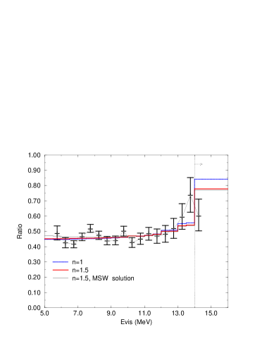
Figure 4: Expected spectra for UN-Gaussian tail out of 3 $\sigma$ with $|1/(E_{vis}-E_{e})|^{n}$ suppression, where the MSW parameters are taken as $\sin^{2}2\theta=0.79$ and $\Delta m^{2}=4\cdot 10^{-5}~{}eV^{2}$ .

Notice that a spectrum by tight cut analysis shows that bins 13-13.5 MeV and 14-20 MeV have no more excess, only bin 13.5-14 MeV still has a “bump” $\!{}^{{\bf?}}$ which can be fully due to a statistic fluctuation. This spectrum is also globally more flat than the regular cut spectrum. It may be another supporting point that the anomaly is from experimental uncertainty.

In conclusion, we have calculated the uncertainty part in high energy bins of the solar neutrino energy spectrum. For a Gaussian energy resolution it is no more than few percent. It seems this is not enough to explain the excess of the 504d data in high energy bins. But it is still a possibility that the excess comes from experimental uncertainty for the 708d data, as well as 825 days data.

References

References

- [1] Y. Suzuki, talk given at 18th International Conference on Neutrino Physics and Astrophysics (NEUTRINO 98), Takayama, Japan, 4-9 Jun 1998; The Super-Kamiokande collaboration, Phys.Rev.Lett. 82 (1999) 2430, hep-ex/9812011.
- [2] J. Bahcall and P. Krastev, Phys.Lett. B436 (1998) 243, hep-ph/9807525.
- [3] V. Berezinsky, G. Fiorentini and M. Lissia, hep-ph/9811352, hep-ph/9904225; A.Yu. Smirnov, Nucl.Phys.Proc.Suppl.70 (1999) 324; V. Barger and K. Whisnant, Phys.Rev.D59 (1999) 093007, hep-ph/9812273; Z. Chacko, R.N. Mohapatra, hep-ph/9905388.
- [4] Q.Y. Liu, talk and transparencies given at the conference: New Era in Neutrino Physics, Tokyo, Japan, 11-12 June 1998.
- [5] M.B. Smy, talk given at the “Division of Particles and Fields Conference”, Los Angeles, 5-9 Jan 1999; Y. Suzuki, talk given at ”17th International Workshop on Weak Interactions and Neutrinos”, Cape Town, South Africa, 24-30 Jan 1999.
- [6] V. Berezinsky, hep-ph/9904259.
- [7] S.P. Mikheyev and A.Yu. Smirnov, Yad. Fiz., 42, 1441 (1985), Nuovo Cim 9C, 17 (1986); L. Wolfenstein, Phys. Rev. D17, 2369 (1978).