Local equilibrium in heavy ion collisions.
Microscopic model versus statistical model analysis.
Abstract
The assumption of local equilibrium in relativistic heavy ion collisions at energies from 10.7A GeV (AGS) up to 160A GeV (SPS) is checked in the microscopic transport model. Dynamical calculations performed for a central cell in the reaction are compared to the predictions of the thermal statistical model. We find that kinetic, thermal, and chemical equilibration of the expanding hadronic matter are nearly approached late in central collisions at AGS energy for fm/ in a central cell. At these times the equation of state may be approximated by a simple dependence . Increasing deviations of the yields and the energy spectra of hadrons from statistical model values are observed for increasing energy, 40A GeV and 160A GeV. These violations of local equilibrium indicate that a fully equilibrated state is not reached, not even in the central cell of heavy ion collisions at energies above 10A GeV. The origin of these findings is traced to the multiparticle decays of strings and many-body decays of resonances.
pacs:
PACS numbers: 25.75.-q, 24.10.Lx, 24.10.Pa, 64.30+tI Introduction
Since the beginning of the 1930s, when cosmic ray cascades of various particles were detected, physicists are trying to describe the process of multiple production of particles in ultrarelativistic collisions of hadrons and nuclei. The idea of Fermi, namely that all secondary particles produced in a Lorentz-contracted volume are in statistical equilibrium [2], was further modified by Pomeranchuk [3]. It was finally developed by Landau into the hydrodynamic theory [4, 5] of multiparticle processes. The most important quantitative predictions of the hydrodynamic theory, such as the dependence of the average particle multiplicity on total energy of the system , the rapidity distributions , violation of Feynman scaling, the mean value of the transverse momentum and its dependence on and the mass of the secondaries, have been verified experimentally. On the other hand, the basic assumptions of the theory, such as the formation of the initial state, the relaxation rate of the system to local equilibrium (LE), the sharpness of the freeze-out (FO) and, finally, the equation of state (EOS) of hot and dense hadronic matter, are based on rough estimates, which have not been rigorously proven yet.
To answer these questions, one can analyze the dynamics provided by microscopic Monte Carlo simulations, i.e., microscopic string, cascade, transport, etc. models. These models describe experimental data on hadronic and nuclear collisions in a wide energy range reasonably well, but do not postulate local equilibrium. Consequently, the EOS and macroscopic variables like temperature, entropy or chemical potential are not implied, but can be calculated, if the system does actually reach LE. For instance, the hypothesis of sharp freeze-out of secondaries in heavy ion collisions was checked by means of three microscopic Monte Carlo models: QGSM [6], RQMD [7] and UrQMD [8]. It was found that these models do neither exhibit a thin or a thick freeze-out layer, which resemble the hyperbolic surface predicted by Bjorken scaling model [9].
The present paper employs the recently developed ultrarelativistic quantum molecular dynamics (UrQMD) model [8, 10] to examine the approach to local equilibrium of hot and dense nuclear matter, produced in central heavy ion collisions at energies from AGS to SPS. Local (and sometimes, in fireball models, even global) equilibrium is the basic ad hoc assumption of the macroscopic hydrodynamic models. It is usually assumed that the nonequilibrium initial stage of nuclear collisions, during which shock waves, partonic jets, etc., heat the system, is considerably shorter than the characteristic hadronization times. Evidently, there must be dissipative and irreversible processes leading to equilibration. One may adopt the scheme of binary collisions, in which the correlation of the many-particle distribution functions, describing highly nonequilibrium states, rapidly sets in [11]. The typical time scale for these processes are collision times, . Then a kinetic stage is approached, where the -body distribution functions are reduced to many one-particle distribution functions, one for each particle species. For time scales sufficiently larger than , the evolution of the system can be described in terms of local average particle number, their velocities and energies. These local average values are the moments of the one-particle distribution functions, and the hydrodynamic stage arises. Other processes, which can cause even faster equilibration, are collective instabilities, convective turbulent transport or chaotic relaxation [12, 13]. They can yield a crude estimate of the relaxation times in the system. On the other hand, multiparticle processes can lead to a delay in reaching equilibrium, because the produced particles are not thermalized. The time scale of the equilibration may appear too long as compared to the typical hadronization times.
As emphasized in [14], according to an UrQMD analysis, it is unlikely that global thermal equilibrium sets in for central Au+Au collisions at the AGS energy. This statement remains true at higher energies also. Figure 1 depicts the time evolution of the baryon density in a single central Pb+Pb collision at 160A GeV. Two disks of baryon rich matter, remnants of the colliding nuclei, consisting mostly of resonances and diquarks, are seen in the fragmentation regions. The volume between the disks becomes more and more baryon dilute, but never purely homogeneous. Apparently, global equilibrium is not reached even in central Pb+Pb collisions at SPS energies. However, the occurrence of LE in the central zone of the heavy ion reaction is still not ruled out.
To verify how close the hot hadronic matter in the cell is to equilibrated matter, one can do a comparison with the statistical model (SM) of a hadron gas [14, 15]. Three parameters, namely, the energy density , the baryon density , and the strangeness density , extracted from the analysis of the cell, are inserted into the equations for an equilibrated ideal gas of hadrons. Then all characteristics of the system in equilibrium, including the yields of different hadronic species, their temperature , and chemical potentials, and , may be calculated unambiguously. If the yields and the energy spectra of the hadrons in the cell are sufficiently close to those of the SM, one can take this as indication for the creation of equilibrated hadronic matter in the central reaction zone.
This method is applied to extract the equation of state (EOS), which connects the pressure and the energy density of the system (generally, either or ). Note that, without the EOS, the system of relativistic hydrodynamic equations, which describe the evolution of hadronic matter, is incomplete. Therefore, the EOS, as extracted from the microscopic model, has a direct impact on the parametrizations used in the macroscopic (hydrodynamic) models.
This paper is organized as follows: a brief description of the UrQMD model is given in Sec. II. Here the necessary and sufficient criteria of local equilibrium are formulated also. It is shown that the hadron distributions in the UrQMD central cell become isotropic at fm/, irrespective of the initial energy of the reaction. This means that kinetic equilibrium is reached. Section III presents the basic equations of the statistical model of the ideal hadronic gas, which is applied for the analysis of the hadron distributions in the central cell. The relaxation of the hadronic matter in the central zone of central heavy ion collisions to thermal and chemical equilibrium is studied in Sec. IV. The UrQMD cell and the SM results are compared for center-of-mass energies of 10.7A GeV (Au+Au, AGS), 40A GeV (Pb+Pb, SPS) and 160A GeV (Pb+Pb, SPS). Finally, the conclusions are drawn in Sec. V.
II Criteria of local equilibrium and conditions in the UrQMD cell
A The UrQMD model
The UrQMD is a microscopic transport model designed for the description of hadron-hadron (), hadron-nucleus () and nucleus-nucleus () collisions for energies spanning a few hundred MeV up to hundreds of GeV per nucleon in the center-of-mass system (c.m. system). The model is presented in detail in [8, 10]. As discrete, quantized degrees of freedom, the model contains 55 baryon and 32 meson states, together with their antiparticles and explicit isospin-projected states, with masses up to 2.25 GeV/. The tables of the experimentally available hadron cross sections, resonance widths and decay modes are implemented as well.
At moderate energies the dynamics of or collisions is described in UrQMD in terms of interactions between the hadrons and their excited states (resonances). At higher values of the four-momentum transfer, interactions cannot be reduced to the hadron-resonance picture anymore, and new excited objects, color strings, come into play. The excitation of the strings make it energetically favorable to break the string into pieces by producing multiple -pairs from the vacuum. Due to the fact that the color string is assumed to be uniformly stretched, the hadrons produced as a result of the string fragmentation will be uniformly distributed in rapidity between the endpoints of the string. The propagation of the hadrons is governed by Hamilton equations of motion, with a binary collision term of the form of relativistic Boltzmann-Uehling-Uhlenbeck (BUU) transport model. The Pauli principle is taken into account via the blocking of the final state, if the outgoing phase space is occupied. No Bose enhancement effects are implemented in the model yet.
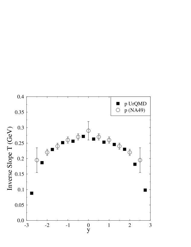
In its present version [16] UrQMD describes the main properties of both hadronic and nuclear interactions [8, 10] reasonably well. Very important for the further analysis is the fact that the UrQMD model reproduces the experimental transverse mass spectra of hadrons in different rapidity intervals, as shown in Fig. 2. The inverse slope parameter, extracted from the Boltzmann fit to the spectra, is directly linked to the temperature in the statistical model. Thus, if the equilibrium conditions (see below) are satisfied, one may estimate the temperature of the cell.
B Preequilibrium stage
Let us first define our system. The sizes of the central zone of perfectly central (impact parameter fm) heavy ion collisions should be neither too small nor too large. The effects caused by the collective flow of particles also can wash out the equilibration picture. In order to diminish number of distorting factors we choose a central cubic cell of volume fm3 centered around the origin of the c.m. system of colliding nuclei. Due to the absence of the preferable direction of the collective motion, the collective velocity of the cell is essentially zero.
Then, to decide whether or not the local equilibrium in the cell is reached, one has to introduce criteria of the equilibrium. In statistical physics the equilibrium state is defined as a state with maximum entropy [17]. However, the direct calculation of the entropy evolution in the cell is notoriously difficult. The cell is not an isolated system. Particles leave it freely, and neither internal energy nor particle number is conserved. Therefore we should apply other, more suitable for this problem, criteria of equilibrium bearing in mind that they are consequences of the general principle of maximum entropy.
We start from the necessary conditions which characterize the preequilibrium stage in the central cell. The flow velocities there should have minimum gradient tending to zero. It means that the local equilibrium in the cell cannot be reached earlier then certain time during which the Lorentz contracted nuclei would have pass through each other. Here is the radius of the nuclei, and the times , typical for each reaction, are 5.46 fm/ (10.7A GeV), 2.9 fm/ (40A GeV), and 1.44 fm/ (160A GeV). After the collective flow of freely streaming hadrons rapidly vanishes.
It looks likely that for the cell of small longitudinal size the pre-equilibrium stage sets in very quickly. For instance, for the central fm3 cell in Pb+Pb collisions at SPS one may expect the equilibration already at fm/. But the detailed analysis shows [15] that the hadronic matter in the different central cells equilibrates at the same rate which does not depend on the longitudinal size of the cell.
Figure 3 presents the average transverse and longitudinal flow of hadrons in 1/8-th of the central cell with the coordinates as a function of time . The longitudinal flow reaches its maximum value at times from fm/ (SPS) to fm/ (AGS). Then it drops and converges to the transverse flow. At fm/ the longitudinal component of the collective flow in the central cell is about 0.1–0.15 only. This corresponds to the temperature distortion MeV. Disappearance of the flow implies (i) isotropy of the velocity distributions, which leads to (ii) isotropy of the diagonal elements of the pressure tensor, calculated from the virial theorem [18],
| (1) |
containing the volume of the cell and the mass and the momentum of the th hadron, and , correspondingly.
The method of moments of the distribution function is a useful tool to investigate irregularities in the particle spectra in high energy physics. Indeed, it is possible to make a conclusion about isotropy of the velocity distributions in terms of the function
| (2) |
where is the th moment of the , , or distribution. The function is a measure of anisotropy of the particle average velocities in longitudinal and transverse directions. The results of the calculations of particle velocity anisotropy of nucleons and pions produced in the central cell at 10.7A GeV, 40A GeV and 160A GeV are given in Fig. 4 for the function . It seems that the velocity distributions becomes isotropic already at fm/. But in equilibrium at energies and temperatures in question hadrons should have Maxwellian, or normal, velocity distribution, which is the only one satisfying the principle of maximum entropy. The distributions of nucleons and pions for all three energies are shown in Fig. 5. One can see that despite the isotropy of collective velocities, the shapes of the distributions become close to the normal one at fm/, not earlier. Therefore, the second moments of the velocity distribution functions are insufficient to study the system anisotropy, and one should apply the moments of higher order.
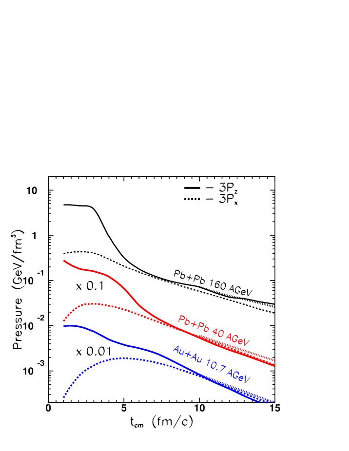
The requirement of isotropy of the velocity distributions is closely related to the requirement of the pressure isotropy. Here the momentum distributions of particles are integrated over the whole number of hadron species, as given by Eq. (1). Figure 6 depicts the time evolution of the pressure in longitudinal and transverse directions calculated for all three energies in question. These components become very close (within the 5%-limit of accuracy) to each other also at fm/. The result does not depend practically on the initial energy of colliding nuclei.
It is worth noting that the appearance of the preequilibrium stage does not imply inevitably that the matter in the cell would be in equilibrium forever. The preequilibrium stage in the cell holds for a period of about fm/ (Fig. 6). Then the system develops again the anisotropy in the pressure and velocity sectors due to significant reduction of number of collisions between particles.
C Criteria of thermal and chemical equilibrium
Suppose conditions (i) and (ii) are fulfilled. Does it mean that the hadronic matter in the cell is in a state close to the equilibrium? No, because both criteria concern the kinetic preequilibrium stage rather than the thermal equilibrium one. Kinetic equilibrium implies isotropy of the velocity distributions of particles (and, therefore, isotropy of pressure) together with the requirement that their velocity distributions must be Maxwellian. Thermal equilibrium indicates that the macroscopic characteristics of the system are nearly equal to their average values. In thermal equilibrium the system is characterized by a unique temperature . Then, the principle of maximum entropy compels the particles of mass to obey the equilibrium distribution function
| (3) |
Here is the momentum of particle, is its chemical potential, sign stands for fermions and for bosons. In the case , where , the Maxwell velocity distribution follows automatically from Eq. (3). Therefore, if the number of particles is conserved, then both definitions of kinetic and thermal equilibrium are equivalent [17, 19]. But in strong interactions at high energies (as well as in chemical reactions) the number of interacting particles and their origin is changed. Thus, the condition of thermal equilibrium should be completed by the requirement of chemical equilibrium. Both criteria read (iii) the distribution functions of hadrons are close to the equilibrium distribution functions, given by Eq. (3) (thermal equilibration), and (iv) the yields of hadrons become saturated (chemical equilibrium) after a certain period. The latter condition assumes that any inverse reaction proceeds with the same rate as the direct reaction. This means, particularly, that the chemical potentials of nonconserved charges vanish, and the chemical potential , assigned to a given particle , is simply
| (4) |
where and denote the baryon charge and strangeness of the particle, and is the baryo- and strangeness chemical potential, respectively.
After the preequilibrium conditions are satisfied, one may address the question on thermal and chemical equilibrium in the cell. But how can we apply the thermostatic criteria to the dynamic picture in the cell, where the internal parameters are instantly changing? The standard procedure [14, 15] is to compare the snapshot of particle yields and spectra in the cell at given time with those predicted by the statistical thermal model of hadron gas [21, 22, 23]. If these spectra are close to each other the hadronic matter in the cell is assumed to reach thermal and chemical equilibrium. The simplicity of the SM has led to a very abundant literature (see, e.g. [24, 25, 26, 27] and references therein). Therefore, we shall recall briefly some of its principle features.
III Statistical model of ideal hadron gas
For the further analysis the thermodynamical parameters of the system, , and , at each step of the time evolution of the colliding system were extracted from the predictions of the statistical model of an ideal hadron gas with the same 55 baryon and 32 meson species and their antistates considered in UrQMD model. As an input the SM uses the total energy density , baryon density and strangeness density , determined within the UrQMD model during the dynamical evolution of the central zone with volume of the A+A system:
| (5) | |||||
| (6) | |||||
| (7) |
Here , are the baryon charge and strangeness of the hadron species , whose particle yields, , and total energy, , are calculated within the SM as:
| (8) | |||||
| (9) |
where , and are the momentum, mass and the degeneracy factor of the hadron species . The distribution function is given by Eq. (3) with the chemical potential . Then, instead of Fermi-Dirac or Bose-Einstein distributions we use for all hadronic species the classical Boltzmann distribution function
| (10) |
At temperatures above 100 MeV the only visible difference (about 10%) between quantum and classical descriptions is in the yields of pions [15].
The hadron pressure given by the statistical model reads
| (11) |
Finally, the entropy density can be calculated for the ideal gas model either by the Gibbs thermodynamical identity
| (12) |
or as a sum over all particles of the product integrated over all possible momentum states
| (13) |
According to the principle of maximum entropy the value of calculated from Eq. (12) or from Eq. (13) represents the maximum value of the entropy density in the system for a given particle composition and given set of microscopic parameters, i.e., energy density, , baryon density, , and strangeness density, .
IV UrQMD versus statistical model. Results and discussion
A Baryon density and strangeness in the cell
As shown in Sec. II, the kinetic equilibrium is attained in the central cell at fm/ for all three reactions. The fraction of non-formed particles at this time is less than 20% and rapidly vanishes. Therefore, fm/ is chosen as a starting point of the direct comparison between UrQMD and SM. Substitution of the values , calculated in the cell for all three reactions in question at fm/, into Eqs. (5)–(7) gives us the key parameters and needed to reproduce particle spectra in the statistical model. The input and output parameters are listed in Tables I–III. Apparently, the conditions in the cell are different for all reactions even at this late stage of the expansion. Because of the different expansion rates the higher temperatures and lower values of the baryonic chemical potential are assigned to the system of heavy ions colliding at SPS energy, which is the highest one in our case. The final time of the calculations may be estimated from the imposed usual hydrodynamic freeze-out conditions, e.g. or GeV/fm3, i.e. 18–20 fm/ for all three reactions. At these times the fraction of already frozen particles in the central cell is about 40–47 %, irrespective on the initial energy of colliding nuclei.
The baryon density in the central zone of the collision at the late stage is not larger than 0.15 fm-3 for all three reactions. Note also that at AGS energies we deal with baryon rich matter, where about 70% of the total energy is carried by baryons, while at SPS most of the energy is deposited in the mesonic sector (more then 70%). At 40A GeV the mesonic and baryonic parts of energy are equal.
At all energies from 10.7A GeV to 160A GeV the total strangeness density of all particles in the central cell is small and negative. This result is independent on the size of the cell [15]. The origin of this effect is quite simple. Strange particles are produced in pairs, for instance, kaons are produced mainly together with lambdas. The total strangeness of the reaction is essentially zero but, owing to small interaction cross section with hadrons, ’s are leaving the central cell much earlier than ’s or ’s. The strangeness density has a minimum somewhere at the maximum overlap of the nuclei and then it relaxes to zero. This evolution behavior of the strangeness density , where and are the strangeness and density of the hadron species , can not be explained by simple combination of e.g. ’s, ’s and ’s, but is defined by contributions of all species, carrying the strange charge. For the ratio (Fig. 7) the behavior is opposite. This ratio rises continuously with time because the baryon density decreases much faster than the strangeness density.
At the early stages of the reaction the strange charge is carried mostly by resonances. At AGS energy the positive strangeness of mesons, mostly ’s, is compensated by the contribution of both baryons (like ’s) and mesons (like ’s), carrying the negative strange charge. It makes the net strangeness density negative, even though small. At SPS energy the contribution of strange baryons to the total strangeness is relatively small, so the difference in strangeness is defined mostly by meson contributions.
To decide whether the strangeness density in the cell is small or not we have also performed calculations for SM with zero strangeness density. As shown in Table IV, although the hadronic yields themselves are only slightly affected by the “symmetrization” of strangeness, their ratios are changed more distinctly. For instance, ratio in the central cell drops from 6.48 to 5.74 at AGS energy, from 2.96 to 2.60 at 40A GeV, and from 1.82 to 1.58 at SPS energy. The total effect is about 15% for all three reactions.
B Isentropic expansion and EOS
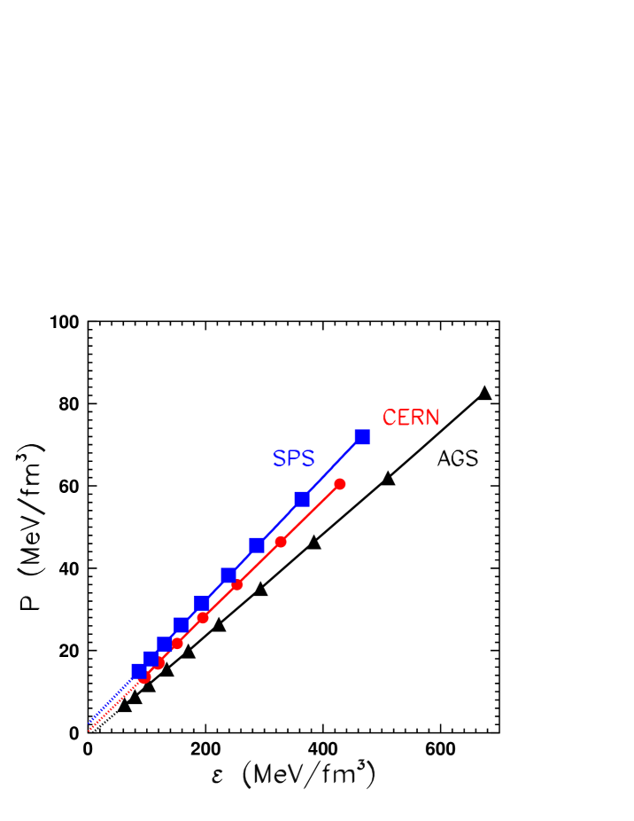
Two other important facts may be gained from the Tables I–III. The entropy per baryon ratio in the cell is almost constant and varies from at AGS to at SPS energy. This result supports the Landau idea of isentropic expansion of a relativistic fluid. The isentropic-like expansion is demonstrated in Fig. 8 which presents the evolution of the central cell in the plane. Also, the fact that the microscopic pressure calculated according to Eq. (1) is nicely reproduced by the Eq. (11) for the pressure of ideal hadron gas [14] favors the applicability of the hydrodynamic description of relativistic heavy ion collisions. The ratio , shown in Fig. 9, is constant for the whole time interval for all three energies. Thus the equation of state, which connects pressure with energy density, has a rather simple form (AGS), 0.13 (40A GeV) and 0.15 (SPS), where corresponds to the speed of sound in the medium. For the ideal ultra-relativistic gas , while the presence of resonances diminishes the sonic velocity to [28], which is in quantitative agreement with our calculations. It is important to stress that the EOS, extracted from the UrQMD analysis of the evolution of hot hadronic matter in the central cell of heavy ion collisions at energies from AGS to SPS, does not contain any kind of softening, which may be associated with the phase transition [29] between the quark-gluon plasma (QGP) and hadronic phase.
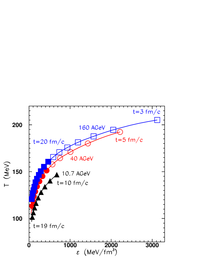
The evolution of the central cell in - plane is shown in Fig. 10. Here, in spite of the absence of indication on the QGP-hadrons phase transition in - plane, we see that the maximal temperature is growing with the initial collision energy and reaches at the beginning of the kinetic equilibrium stage the zone of the phase transition predicted by the MIT bag model for ideal QGP phase with . At earlier times the determination of temperature in the cell by means of the SM fit is doubtful, since the necessary conditions of local equilibrium are not satisfied.
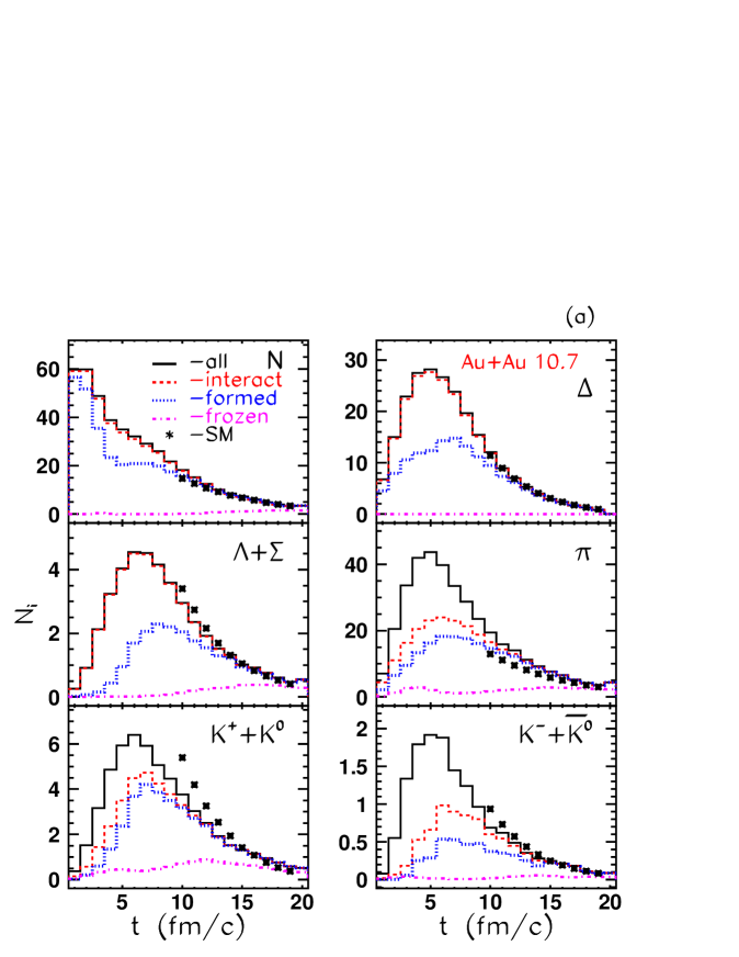
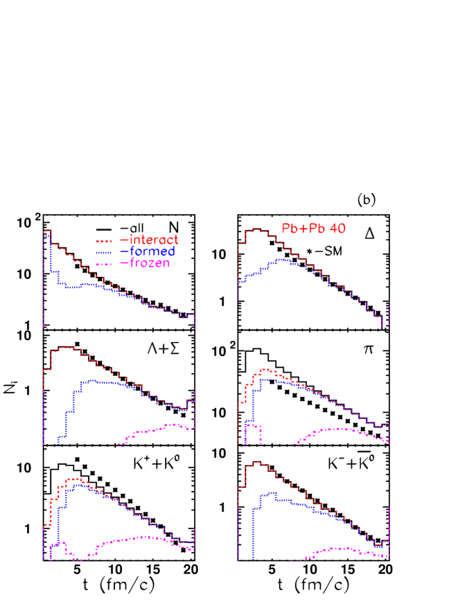
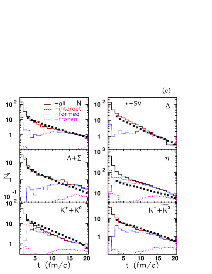
C Hadron yields and energy spectra
To complete the analysis of local equilibrium in the central cell we should make a comparison between hadron yields and spectra obtained in the both models. If the number of particles in the cell and their energy spectra are very close to those predicted by the SM, one may conclude that the thermal and chemical equilibrium is reached. The yields of different hadrons in the central fm3 cell are shown in Figs. 11(a)–(c) (see also Table IV) for central (impact parameter ) heavy ion collisions at 10.7A GeV, 40A GeV and 160A GeV, respectively. We see that for baryons at fm/ the agreement between the SM and UrQMD results is reasonably good. For pions and kaons the yields differ drastically, especially at 160A GeV. Compared to UrQMD, the statistical model significantly underestimates the number of pions and overestimates the kaon yield. This difference in the pion yield cannot be explained only by the many-body () decays of resonances, whose number is lower in the UrQMD calculations as seen in Fig. 12. In fact, the main discrepancy is observed for pions and many-body decaying resonances, like , etc. Statistical model overestimates the production of such resonances and underestimates the yield of pions. The enhancement of the resonances, however, can describe only 20% of difference in pion yields, the other 80% are coming via the multiparticle processes, i.e., fragmentations of strings. The condition (iv) is not satisfied and, therefore, the hadronic matter in the UrQMD central cell is not chemically equilibrated.
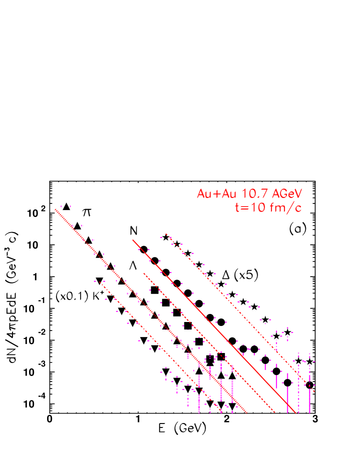
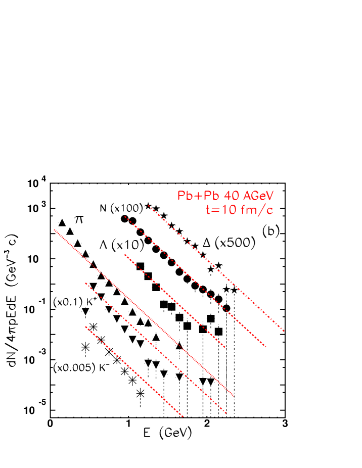
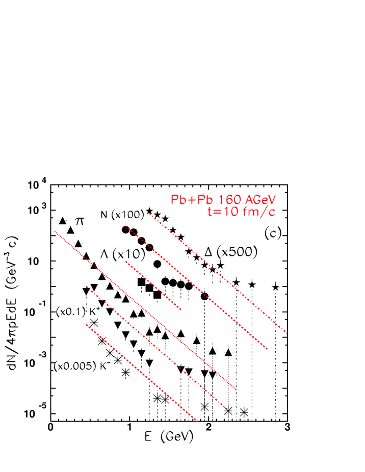
To verify how good the SM reproduces the temperature of the system we display in Figs. 13(a)-13(c) the energy spectra of different hadronic species, obtained from the microscopic calculations. The predictions of the statistical model are plotted onto the particle spectra, too. Again, at AGS energy the difference between the UrQMD and SM results for baryons lies within the 10%- range of accuracy. With the rise of initial energy from AGS to SPS the agreement between the models in the baryonic sector becomes worse. Pion energy spectra demonstrate the same tendency. Moreover, even at 10.7A GeV the deviations of pion spectra in UrQMD from those of the SM are significant. The Boltzmann fit to pion and nucleon energy spectra from the central cell has been performed at 160A GeV, where the deviations from the SM predictions are especially noticeable. Results of the fit are listed in Table V. We see that the nucleon “temperature” is always 30–40 MeV below the temperature obtained in the statistical model. For pions the difference is more dramatic: 50–60 MeV, although the UrQMD energy spectra themselves agree well with the exponential form of Boltzmann distribution.
But maybe all these nonequilibrium effects are caused solely by pions which, due to their simultaneous production in inelastic collisions and decays of resonances, are the only hadrons not thermally and chemically equilibrated? Indeed, from Fig. 14, which depicts the evolution of the average number of collisions per particle in the cell at SPS energy, it follows that pions have undergone about 1.6–1.7 elastic collisions while baryons have suffered more than 20 strong interactions. Thus, it would be expected that without pions the SM will predict much lower temperature which will agree with that of the UrQMD. To check this hypothesis we subtract the energy in the cell carried by pions from the total energy of hadrons. Then we substitute the new value of the energy density together with the unchanged values of baryon and strangeness densities into the SM fit to the UrQMD data, and impose the requirement of absence of pions. Results of the fit are listed in Table VI for Pb+Pb at 160A GeV at fm/. Although the number of pions in the cell is almost two times larger than that of SM, it appears that, due to lower temperature of pions in UrQMD, the total excess of pion energy density in the cell is 24 MeV/fm3, or about of the total pion energy density given by the statistical model. The contamination of pion fraction does not decrease the temperature in the SM. Instead, it leads to the increase of chemical potential of strange particles.
Therefore, despite the occurrence of a state in which hadrons are in kinetic equilibrium and collective flows are very small, the hadronic matter is neither in thermal nor in chemical equilibrium. This state of hot hadronic matter is very peculiar [30] and the results of the investigations will be published elsewhere [31]. Similar results have been obtained in [32], where the central region of ultra-relativistic Au+Au collisions at RHIC energy was studied using the parton cascade model [20]. It was found that, despite approaching kinetic equilibrium in the system, the chemical composition of quarks and gluons was not in chemical equilibrium. Our analysis shows also that the extraction of temperature by performing the SM fit to hadron yields and energy spectra is a very delicate procedure. If the whole system is out of the equilibrium state, than the “apparent” temperatures obtained from the fit may occur high enough to hit the zone of quark-hadron phase transition or even pure QGP phase (Fig. 10, open symbols).
V Conclusions
The results of the present study may be summarized as follows. We used the microscopic transport UrQMD model to verify the appearance of the local equilibrium in the central zone of heavy ion collisions at relativistic energies, spanning from AGS to SPS. To analyze the results of the dynamical calculations the traditional methodic has been applied. First, the conditions of preequilibrium kinetic stage have been checked by means of the isotropy of the pressure and velocity distributions. It is shown that the kinetic equilibrium is reached by hadronic matter in the central fm3 cell at about fm/ for a not very long period, fm/. Secondly, the values of the energy density, baryonic density and strangeness density, calculated microscopically, were used as an input to calculate temperature as well as baryonic and strangeness chemical potentials within the statistical model of ideal hadron gas.
The total strangeness of all hadronic species carrying strangeness charge in the central cell is shown to be negative though small. This is because of the fact that ’s escape from the interaction zone much easier than ’s or ’s due to their small interaction cross section with hadrons. The small negative strangeness of the central cell, however, cannot be neglected because it affects the ratios of strange particles, like .
It is worth to note that due to rather complicated dynamics of heavy ion collisions thermal models cannot fully describe the bulk of experimental data [33]. In contrast, in the symmetric central zone of the heavy ion collisions almost all dynamical factors are reduced. This gives us a chance to study the relaxation of the hot hadronic matter to the thermal and chemical equilibrium, provided it would set in within the hadronization time of the system.
We found that the entropy per baryon in the central cell remains constant at the late stage of the expansion for energies varying from 10.7A GeV to 160A GeV. This circumstance formally supports the application of the relativistic hydrodynamical model. But the further comparison between the predictions of the microscopic and macroscopic models reveals significant discrepancies in the yields and energy spectra of hadrons. Compared to UrQMD, the statistical model underestimates, for instance, the number of pions. This “meson problem” is not a feature attributed solely to the particular microscopic model like UrQMD. Experimental data on pion yields at SPS energies [34] show unambiguously the enhancement of pions compared to the SM calculations. Several possible solutions have been suggested recently. Admitting that the hot hadronic matter appears not in the state of chemical equilibrium, one may implement the effective chemical potential for pions (and other species, too) [35, 36]. In that case the state of maximum entropy is not reached [36] yet.
Also, the temperatures of different hadronic species are not the same. The differences between the UrQMD and SM results increase with the rise of initial energy of colliding nuclei. Pions seem to have the lowest temperature and nucleons the highest one among all hadron species. Both, the pion and nucleon temperatures in the cell in Pb+Pb collisions at SPS energy are always far below the temperature predicted by the statistical thermal model.
The information at hand permits us to summarize that, in contrast to low energies, local thermal and chemical equilibrium (in the sense of the thermal model) is not obtained even in the central zone of heavy ion collisions at energies above 10.7A GeV in the UrQMD simulations. The hadronic matter in the UrQMD model seems not to evolve towards the state of maximum entropy, and this fact deserves to be investigated in detail.
Acknowledgments
We would like to thank L. Csernai, U. Heinz, J. Rafelski, L. Satarov, E. Shuryak, J. Stachel, and N. Xu for the helpful discussions and comments. L.B. and E.Z. are grateful to the Institute for Theoretical Physics, University of Frankfurt for the warm and kind hospitality. This work was supported by the Graduiertenkolleg für Theoretische und Experimentelle Schwerionenphysik, Frankfurt–Giessen, the Bundesministerium für Bildung und Forschung, the Gesellschaft für Schwerionenforschung, Darmstadt, Deutsche Forschungsgemeinschaft, and the Alexander von Humboldt–Stiftung, Bonn.
REFERENCES
- [1]
- [2] E. Fermi, Prog. Theor. Phys. 5, 570 (1950); Phys. Rev. 81, 683 (1951).
- [3] I.Ja. Pomeranchuk, Dokl. Akad. Nauk (USSR) 78, 889 (1951).
- [4] L.D. Landau, Izv. Akad. Nauk SSSR, Ser. Fiz. 17, 51 (1953).
- [5] S.Z. Belenkij and L.D. Landau, Nuovo Cimento Suppl. 3, 15 (1956).
- [6] L.V. Bravina, I.N. Mishustin, A.N. Amelin, J. Bondorf, and L.P. Csernai, Phys. Lett. B 354, 196 (1995); Heavy Ion Phys. 5, 455 (1997).
- [7] H. Sorge, Phys. Lett. B 373, 16 (1996).
- [8] S.A. Bass, M. Belkacem, M. Bleicher, M. Brandstetter, L. Bravina, C. Ernst, L. Gerland, M. Hofmann, S. Hofmann, J. Konopka, G. Mao, L. Neise, S. Soff, C. Spieles, H. Weber, L.A. Winckelmann, H. Stöcker, W. Greiner, Ch. Hartnack, J. Aichelin, and N. Amelin, Prog. Part. Nucl. Phys. 41, 225 (1998).
- [9] J.D. Bjorken, Phys. Rev. D 27, 140 (1983).
- [10] M. Bleicher, E. Zabrodin, C. Spieles, S.A. Bass, C. Ernst, S. Soff, L. Bravina, H. Weber, H. Stöcker, and W. Greiner, J. Phys. G 25 (1999) (in press).
- [11] N.N. Bogolyubov, J. Phys. (USSR) 10, 256 (1946); in Studies in Statistical Mechanics, Vol. 1, edited by D. de Boer and G. E. Uhlenbeck (North-Holland, Amsterdam, 1962), p. 1.
- [12] H. Stöcker and W. Greiner, Phys. Rep. 137, 277 (1986).
- [13] P. Carruthers, in Local Equilibrium in Strong Interaction Physics, edited by D.K. Scott and R.M. Weiner (World Scientific, Singapore, 1985), p. 390.
- [14] L.V. Bravina, M.I. Gorenstein, M. Belkacem, S.A. Bass, M. Bleicher, M. Brandstetter, M. Hofmann, S. Soff, C. Spieles, H. Weber, H. Stöcker, and W. Greiner, Phys. Lett. B 434, 379 (1998).
- [15] L.V. Bravina, M. Brandstetter, M.I. Gorenstein, E.E. Zabrodin, M. Belkacem, M. Bleicher, S.A. Bass, C. Ernst, M. Hofmann, S. Soff, H. Stöcker, and W. Greiner, J. Phys. G 25, 351 (1999).
- [16] UrQMD1.1, http://www.th.physik.uni-frankfurt.de/ urqmd/urqmd.html
- [17] L.D. Landau, E.M. Lifshitz, and L.P. Pitaevskii, Statistical Physics (Pergamon, New York, 1980), Part 1.
- [18] M. Berenguer, C. Hartnack, G. Peilert, H. Stöcker, W. Greiner, J. Aichelin, and A. Rosenhauer, J. Phys. G 18, 655 (1992).
- [19] S. de Groot, W.A. van Leuwen, and C.G. van Weert, Relativistic Kinetic Theory (North-Holland, Amsterdam, 1980).
- [20] K. Geiger, Phys. Rep. 258, 237 (1995).
- [21] H. Stöcker, A.A. Ogloblin, and W. Greiner, Z. Phys. A 303, 259 (1981).
- [22] M.I. Gorenstein, H.G. Miller, R.M. Quick, and S.N. Yang, Phys. Rev. C 50, 2232 (1994).
- [23] J. Cleymans, D. Elliot, H. Satz, and R.L. Thews, Z. Phys. C 74, 319 (1997).
- [24] R. Hagedorn, Nuovo Cimento Suppl. 3, 147 (1965); R. Hagedorn and J. Rafelski, Phys. Lett. B 97, 136 (1980).
- [25] P. Braun-Munzinger, J. Stachel, J.P. Wessels, and N. Xu, Phys. Lett. B 365, 1 (1996).
- [26] F. Becattini, Z. Phys. C 69, 485 (1996).
- [27] M. Belkacem, M. Brandstetter, S.A. Bass, M. Bleicher, L. Bravina, M.I. Gorenstein, J. Konopka, L. Neise, C. Spieles, S. Soff, H. Weber, H. Stöcker, and W. Greiner, Phys. Rev. C 58, 1727 (1998).
- [28] E. Shuryak, Yad. Fiz. 16, 707 (1972) [Sov. J. Nucl. Phys. 16, 395 (1973)].
- [29] C.M. Hung and E. Shuryak, Phys. Rev. Lett. 75, 4003 (1995); Phys. Rev. C 56, 453 (1997).
- [30] E.E. Zabrodin, L.V. Bravina, H. Stöcker, and W. Greiner, hep-ph/9901356.
- [31] L.V. Bravina et al. (unpublished).
- [32] K. Geiger and J.I. Kapusta, Phys. Rev. D 47, 4905 (1993).
- [33] U. Heinz, J. Phys. G 25, 263 (1999).
- [34] S.V. Afanasjev et al., NA49 Collaboration, Nucl. Phys. A610, 188c (1996); C. Borman et al., NA49 Collaboration, J. Phys. G 23, 1817 (1997).
- [35] G.D. Yen and M.I. Gorenstein, Phys. Rev. C 59, 2788 (1999).
- [36] J. Letessier and J. Rafelski, Phys. Rev. C 59, 947 (1999).


(b) The same as (a) but for Pb+Pb collisions at 40A GeV at 6 fm/ (upper frame) and at 8 fm/ (lower frame).
(c) The same as (a) but for Pb+Pb collisions at 160A GeV at 5 fm/ (upper frame) and at 8 fm/ (lower frame).


(b) The same as (a) but for Pb+Pb collisions at 40A GeV.
(c) The same as (a) but for Pb+Pb collisions at 160A GeV.

(b) The same as (a) but for Pb+Pb collisions at 40A GeV. Parameters of the Boltzmann fit are =151 MeV, =345 MeV, and =74 MeV.
(c) The same as (a) but for Pb+Pb collisions at 160A GeV. Parameters of the Boltzmann fit are =161 MeV, =197 MeV, and =36.8 MeV.

| Time | |||||||||
|---|---|---|---|---|---|---|---|---|---|
| fm/ | MeV/fm3 | fm-3 | fm-3 | MeV | MeV | MeV | MeV/fm3 | fm-3 | |
| 10 | 674.8 | 0.332 | -0.0078 | 128.46 | 146.74 | 510.03 | 82.67 | 4.01 | 12.07 |
| 11 | 510.7 | 0.261 | -0.0070 | 122.06 | 140.15 | 519.16 | 61.99 | 3.12 | 11.95 |
| 12 | 384.4 | 0.204 | -0.0055 | 116.37 | 133.87 | 526.73 | 46.41 | 2.42 | 11.90 |
| 13 | 293.4 | 0.160 | -0.0037 | 112.38 | 127.94 | 534.51 | 35.06 | 1.90 | 11.86 |
| 14 | 222.5 | 0.125 | -0.0028 | 107.37 | 122.12 | 542.13 | 26.35 | 1.48 | 11.82 |
| 15 | 170.5 | 0.100 | -0.0029 | 100.73 | 116.22 | 553.56 | 19.88 | 1.16 | 11.62 |
| 16 | 134.0 | 0.081 | -0.0024 | 95.94 | 111.42 | 560.33 | 15.47 | 0.94 | 11.59 |
| 17 | 102.5 | 0.063 | -0.0026 | 86.85 | 106.28 | 566.99 | 11.69 | 0.74 | 11.56 |
| 18 | 79.56 | 0.051 | -0.0024 | 78.90 | 101.46 | 574.17 | 8.83 | 0.58 | 11.55 |
| Time | |||||||||
|---|---|---|---|---|---|---|---|---|---|
| fm/ | MeV/fm3 | fm-3 | fm-3 | MeV | MeV | MeV | MeV/fm3 | fm-3 | |
| 10 | 428.6 | 0.146 | -0.0063 | 151.11 | 344.97 | 74.03 | 60.47 | 2.90 | 19.76 |
| 11 | 327.9 | 0.116 | -0.0056 | 145.15 | 355.60 | 69.72 | 46.44 | 2.29 | 19.78 |
| 12 | 253.3 | 0.093 | -0.0038 | 139.65 | 367.50 | 68.41 | 36.00 | 1.83 | 19.77 |
| 13 | 195.3 | 0.073 | -0.0047 | 134.13 | 375.42 | 60.13 | 27.93 | 1.46 | 19.97 |
| 14 | 151.6 | 0.059 | -0.0036 | 128.77 | 388.19 | 57.76 | 21.74 | 1.17 | 19.95 |
| 15 | 118.9 | 0.048 | -0.0030 | 123.45 | 404.47 | 55.82 | 17.01 | 0.94 | 19.65 |
| 16 | 95.4 | 0.040 | -0.0022 | 118.52 | 422.08 | 56.00 | 13.55 | 0.78 | 19.21 |
| 17 | 74.0 | 0.033 | -0.0024 | 113.26 | 437.23 | 49.81 | 10.46 | 0.62 | 18.94 |
| 18 | 59.88 | 0.027 | -0.0028 | 109.06 | 447.99 | 41.27 | 8.43 | 0.51 | 18.82 |
| Time | |||||||||
|---|---|---|---|---|---|---|---|---|---|
| fm/ | MeV/fm3 | fm-3 | fm-3 | MeV | MeV | MeV | MeV/fm3 | fm-3 | |
| 10 | 467.0 | 0.092 | -0.0099 | 160.564 | 196.64 | 36.78 | 71.91 | 3.24 | 35.13 |
| 11 | 364.0 | 0.073 | -0.0077 | 155.208 | 202.76 | 34.73 | 56.76 | 2.61 | 35.83 |
| 12 | 287.0 | 0.056 | -0.0057 | 150.467 | 202.90 | 32.04 | 45.55 | 2.13 | 37.85 |
| 13 | 239.0 | 0.049 | -0.0067 | 146.453 | 215.20 | 28.71 | 38.29 | 1.82 | 36.86 |
| 14 | 193.0 | 0.039 | -0.0067 | 142.419 | 212.18 | 22.27 | 31.46 | 1.51 | 39.41 |
| 15 | 158.0 | 0.031 | -0.0044 | 138.531 | 216.93 | 23.23 | 26.19 | 1.28 | 41.04 |
| 16 | 130.0 | 0.029 | -0.0037 | 133.837 | 245.73 | 25.20 | 21.51 | 1.08 | 37.56 |
| 17 | 106.9 | 0.023 | -0.0037 | 130.165 | 249.13 | 20.46 | 17.96 | 0.91 | 39.14 |
| 18 | 86.9 | 0.018 | -0.0029 | 126.450 | 251.17 | 18.34 | 14.89 | 0.77 | 41.68 |
| Hadrons | 10.7A GeV | 40A GeV | 160A GeV | ||||||
|---|---|---|---|---|---|---|---|---|---|
| SM | UrQMD | SM | UrQMD | SM | UrQMD | ||||
| =0 | =0 | =0 | |||||||
| 12.90 | 12.99 | 19.40 | 14.35 | 14.41 | 26.65 | 17.43 | 17.47 | 33.02 | |
| 14.93 | 14.70 | 18.19 | 5.81 | 5.69 | 5.72 | 3.28 | 3.20 | 2.53 | |
| 11.53 | 11.40 | 12.08 | 4.73 | 4.64 | 5.86 | 2.97 | 2.89 | 4.17 | |
| 3.24 | 3.40 | 2.95 | 1.94 | 2.03 | 2.11 | 1.51 | 1.58 | 1.17 | |
| 3.06 | 3.22 | 2.72 | 1.98 | 2.08 | 1.94 | 1.79 | 1.88 | 1.90 | |
| 0.54 | 0.60 | 0.21 | 0.51 | 0.57 | 0.31 | 0.57 | 0.64 | 0.37 | |
| 5.68 | 5.40 | 3.77 | 4.54 | 4.28 | 3.24 | 4.84 | 4.50 | 2.98 | |
| 2.98 | 2.85 | 2.31 | 2.65 | 2.50 | 2.65 | 3.39 | 3.18 | 3.40 | |
| 0.88 | 0.94 | 0.69 | 1.53 | 1.65 | 1.43 | 2.64 | 2.84 | 2.17 | |
| 0.48 | 0.52 | 0.30 | 0.91 | 0.98 | 0.76 | 1.88 | 2.03 | 1.95 | |
| 0.19 | 0.19 | 0.00 | 0.059 | 0.058 | 0.013 | 0.223 | 0.216 | 0.13 | |
| 0.18 | 0.18 | 0.00 | 0.060 | 0.059 | 0.025 | 0.264 | 0.256 | 0.10 | |
| Time | |||
|---|---|---|---|
| fm/ | MeV | MeV | MeV |
| 10 | 160.56 | ||
| 11 | 155.21 | ||
| 12 | 150.47 | ||
| 13 | 146.45 | ||
| 14 | 142.42 | ||
| 15 | 138.53 |
| MeV/fm3 | fm-3 | fm-3 | MeV | MeV | MeV | |
|---|---|---|---|---|---|---|
| With pions | 467.0 | 0.0924 | -0.00986 | 160.56 | 196.64 | 36.78 |
| Without pions | 369.0 | 0.0924 | -0.00986 | 160.50 | 195.50 | 48.61 |