FZJ-IKP(Th)-1999-16

We develop a formalism for evaluation of the transverse momentum dependence of cross sections of the radiation processes in medium. The analysis is based on the light-cone path integral approach to the induced radiation. The results are applicable in both QED and QCD.

It is well known that at high energies the multiple scattering can considerably modify cross sections of the radiation processes in medium [1, 2]. Recently this effect (called the Landau-Pomeranchuk-Migdal (LPM) effect) in QED and QCD has attracted much attention [3, 4, 5, 6, 7, 8, 9, 10] (see also [11] and references therein). In [6] we have developed a new rigorous light-cone path integral approach to the LPM effect. There we have discussed the $p_{T}$-integrated spectra. For many problems it is highly desirable to have also a formalism for the $p_{T}$-dependence of the radiation rate. In the present paper we derive the corresponding formulas. Similarly to [6] our results are applicable in both QED and QCD.

For simplicity we describe the formalism for an induced $a\rightarrow bc$ transition in QED for scalar particles with an interaction Lagrangian $L_{int}=\lambda[\hat{\psi}_{b}^{+}\hat{\psi}_{c}^{+}\hat{\psi}_{a}+\hat{\psi}_{a}^{+}\hat{\psi}_{c}\hat{\psi}_{b}]$ (it is assumed that $m_{a}<m_{b}+m_{c}$, and the decay $a\rightarrow bc$ in vacuum is absent). The $S$-matrix element for the $a\rightarrow bc$ transition in an external potential reads

$$\langle bc|\hat{S}|a\rangle=i\int\!dtd\mbox{{\bf r}}\lambda\psi_{b}^{*}(t,\mbox{{\bf r}})\psi_{c}^{*}(t,\mbox{{\bf r}})\psi_{a}(t,\mbox{{\bf r}})\,,$$ (1)

where $\psi_{i}$ are the wavefunctions (incoming for $i=a$ and outgoing for $i=b,c$). We write $\psi_{i}$ as

$$\psi_{i}(t,\mbox{{\bf r}})=\frac{1}{\sqrt{2E_{i}}}\exp[-i(t-z)p_{i,z}]\phi_{i}(t,\mbox{{\bf r}})\,.$$ (2)

We consider the case when the particle $a$ approaches the target from infinity, and normalize the flux to unity (it corresponds to $|\phi_{i}|=1$) at $z=-\infty$ for $i=a$ and at $z=\infty$ for $i=b,c$. The case when the particle $a$ is produced in a hard reaction in a medium (or at finite distance from a medium) will be discussed later. At high energy, $E_{i}\gg m_{i}$, the dependence of $\phi_{i}$ on the variable $\tau=(t+z)/2$ at $t-z=$const is governed by the two-dimensional Schrödinger equation

$$i\frac{\partial{\phi_{i}}}{\partial{\tau}}=H_{i}\phi_{i}\,,$$ (3)

$$H_{i}=-\frac{1}{2\mu_{i}}\left(\frac{\partial}{\partial\mbox{{\boldmath$\rho$}}}\right)^{2}+e_{i}U+\frac{m_{i}^{2}}{2\mu_{i}}\,,$$ (4)

where $\mu_{i}=p_{i,z}$, $\rho$ is the transverse coordinate, $e_{i}$ is the electric charge, and $U$ is the potential of the target.

In the high energy limit from (1), (2) one can obtain for the inclusive cross section

$$\frac{d^{5}\sigma}{dxd\mbox{{\bf q}}_{b}d\mbox{{\bf q}}_{c}}=\frac{2}{(2\pi)^{4}}\mbox{Re}\!\int\!d\mbox{{\boldmath$\rho$}}_{1}d\mbox{{\boldmath$\rho$}}_{2}\!\!\int\limits_{z_{1}<z_{2}}\!\!dz_{1}dz_{2}\,g\langle F(z_{1},\mbox{{\boldmath$\rho$}}_{1})F^{*}(z_{2},\mbox{{\boldmath$\rho$}}_{2})\rangle\,,$$ (5)

where $\left.F(z,\mbox{{\boldmath$\rho$}})=\phi_{b}^{*}(t,\mbox{{\bf r}})\phi_{c}^{*}(t,\mbox{{\bf r}})\phi_{a}(t,\mbox{{\bf r}})\right|_{t=z}\,,$ $\mbox{{\bf q}}_{b,c}$ are the transverse momenta, $x=p_{b,z}/p_{a,z}$ (note that for the particle $c$ $p_{c,z}=(1-x)p_{a,z}$), $g=\lambda^{2}/[16\pi x(1-x)E_{a}^{2}]$, $\langle...\rangle$ means averaging over the states of the target. Since the wavefunctions enter (5) only at $t=z$, $\phi_{i}$ can be regarded as functions of $z$, and $\rho$. In the Schrödinger equation (3) $z$ will play the role of time. We represent the $z$-dependence of $\phi_{i}$ in terms of the Green’s function, $K_{i}$, of the Hamiltonian (4). Then, diagrammatically, (5) is described by the graph of Fig. 1a. We depict $K_{i}$ ($K_{i}^{*}$) by $\rightarrow$ ($\leftarrow$). The dotted line shows the transverse density matrices at large longitudinal distances in front of ($z=z_{i}$) and behind ($z=z_{f}$) the target.

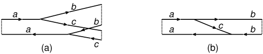
Figure 1: The diagram representation of the inclusive spectrum (5) (a), and (7) (b).

We will consider first the $\mbox{{\bf q}}_{c}$-integrated spectrum. For the sake of generality we assume that all the particles are charged in this case. Later we will give the formula for the totally inclusive spectrum when at least one of the final particles has a zero charge. For the $\mbox{{\bf q}}_{c}$-integrated case the transverse density matrix for the final particle $c$ is given by a $\delta$-function, and taking advantage of the relation

$$\int\!d\mbox{{\boldmath$\rho$}}_{2}K(\mbox{{\boldmath$\rho$}}_{2},z_{2}|\mbox{{\boldmath$\rho$}}_{1},z_{1})K^{*}(\mbox{{\boldmath$\rho$}}_{2},z_{2}|\mbox{{\boldmath$\rho$}}_{1}^{{}^{\prime}},z_{1})=\delta(\mbox{{\boldmath$\rho$}}_{1}-\mbox{{\boldmath$\rho$}}_{1}^{{}^{\prime}})$$ (6)

one can transform the graph of Fig. 1a into that of Fig. 1b. The corresponding analytical expression reads

$$\frac{d^{3}\sigma}{dxd\mbox{{\bf q}}_{b}}=\frac{2}{(2\pi)^{2}}\mbox{Re}\!\!\int\!\!d\mbox{{\boldmath$\rho$}}_{b,f}d\mbox{{\boldmath$\rho$}}_{b,f}^{{}^{\prime}}d\mbox{{\boldmath$\rho$}}_{b}d\mbox{{\boldmath$\rho$}}_{b}^{{}^{\prime}}d\mbox{{\boldmath$\rho$}}_{a}d\mbox{{\boldmath$\rho$}}_{a}^{{}^{\prime}}d\mbox{{\boldmath$\rho$}}_{a,i}d\mbox{{\boldmath$\rho$}}_{a,i}^{{}^{\prime}}\exp[-i\mbox{{\bf q}}_{b}(\mbox{{\boldmath$\rho$}}_{b,f}-\mbox{{\boldmath$\rho$}}_{b,f}^{{}^{\prime}})]\!\int\limits_{z_{i}}^{z_{f}}\!\!dz_{1}\!\!\int\limits_{z_{1}}^{z_{f}}\!\!dz_{2}$$

$$\times\,gS_{b}(\mbox{{\boldmath$\rho$}}_{b,f},\mbox{{\boldmath$\rho$}}_{b,f}^{{}^{\prime}},z_{f}|\mbox{{\boldmath$\rho$}}_{b},\mbox{{\boldmath$\rho$}}_{b}^{{}^{\prime}},z_{2})M(\mbox{{\boldmath$\rho$}}_{b},\mbox{{\boldmath$\rho$}}_{b}^{{}^{\prime}},z_{2}|\mbox{{\boldmath$\rho$}}_{a},\mbox{{\boldmath$\rho$}}_{a}^{{}^{\prime}},z_{1})S_{a}(\mbox{{\boldmath$\rho$}}_{a},\mbox{{\boldmath$\rho$}}_{a}^{{}^{\prime}},z_{2}|\mbox{{\boldmath$\rho$}}_{a,i},\mbox{{\boldmath$\rho$}}_{a,i}^{{}^{\prime}},z_{i})\,,\,\,\,\,\,\,\,\,\,\,\,\,\,\,\,\,$$ (7)

where

$$S_{i}(\mbox{{\boldmath$\rho$}}_{2},\mbox{{\boldmath$\rho$}}_{2}^{{}^{\prime}},z_{2}|\mbox{{\boldmath$\rho$}}_{1},\mbox{{\boldmath$\rho$}}_{1}^{{}^{\prime}},z_{1})=\langle K_{i}(\mbox{{\boldmath$\rho$}}_{2},z_{2}|\mbox{{\boldmath$\rho$}}_{1},z_{1})K_{i}^{*}(\mbox{{\boldmath$\rho$}}_{2}^{{}^{\prime}},z_{2}|\mbox{{\boldmath$\rho$}}_{1}^{{}^{\prime}},z_{1})\rangle$$ (8)

is the evolution operator for the transverse density matrix, and the factor $M$ is given by

$$M(\mbox{{\boldmath$\rho$}}_{2},\mbox{{\boldmath$\rho$}}_{2}^{{}^{\prime}},z_{2}|\mbox{{\boldmath$\rho$}}_{1},\mbox{{\boldmath$\rho$}}_{1}^{{}^{\prime}},z_{1})=\langle K_{b}(\mbox{{\boldmath$\rho$}}_{2},z_{2}|\mbox{{\boldmath$\rho$}}_{1},z_{1})K_{c}(\mbox{{\boldmath$\rho$}}_{2}^{{}^{\prime}},z_{2}|\mbox{{\boldmath$\rho$}}_{1},z_{1})K_{a}^{*}(\mbox{{\boldmath$\rho$}}_{2}^{{}^{\prime}},z_{2}|\mbox{{\boldmath$\rho$}}_{1}^{{}^{\prime}},z_{1})\rangle\,.$$ (9)

We assume that the target density does not depend on $\rho$. Then a considerable part of calculations can be done analytically. In (8), (9) we represent the Green’s functions in the path integral form. In the corresponding path integral formulas for $S_{i}$ and $M$ the interaction of the particles with the target potential after averaging over the target states turns out to be transformed into the interaction between trajectories described by the Glauber absorption factors. For $S_{i}$ the corresponding absorption cross section is given by the dipole cross section $\sigma_{i\bar{i}}$ of interaction with the medium constituent of $i\bar{i}$ pair. The absorption factor for $M$ involves the three-body cross section $\sigma_{\bar{a}bc}$ depending on the relative transverse vectors $\mbox{{\boldmath$\tau$}}_{bc}=\mbox{{\boldmath$\rho$}}_{b}-\mbox{{\boldmath$\rho$}}_{c}$ and $\mbox{{\boldmath$\tau$}}_{ab}=\mbox{{\boldmath$\rho$}}_{a}-\mbox{{\boldmath$\rho$}}_{b}$. The factor $S_{i}$ can be evaluated analytically. The corresponding formulas are given in [12, 6]. The factor $M$ after the analytical path integration over the center-of-mass coordinates can be expressed through the Green’s function $K_{bc}$ describing the relative motion of the particles $b$ and $c$ in a fictitious $\bar{a}bc$ system. The formula for $M$ can be obtained from that given in [6] by replacing the final transverse coordinate $\mbox{{\boldmath$\rho$}}_{2}$ by $\mbox{{\boldmath$\rho$}}_{2}^{{}^{\prime}}$ for the particle $c$. The expression for the probability of the $a\rightarrow bc$ transition at a given impact parameter which we obtain integrating analytically over all the transverse coordinates (except for $\mbox{{\boldmath$\tau$}}_{b}=\mbox{{\boldmath$\rho$}}_{b,f}-\mbox{{\boldmath$\rho$}}_{b,f}^{{}^{\prime}}$) in (7) has the form

$$\frac{d^{3}P}{dxd\mbox{{\bf q}}_{b}}=\frac{2}{(2\pi)^{2}}\mbox{Re}\!\!\int\!\!d\mbox{{\boldmath$\tau$}}_{b}\,\exp(-i\mbox{{\bf q}}_{b}\mbox{{\boldmath$\tau$}}_{b})\!\!\int\limits_{z_{i}}^{z_{f}}\!\!dz_{1}\!\!\int\limits_{z_{1}}^{z_{f}}\!\!dz_{2}\,g\Phi_{b}(\mbox{{\boldmath$\tau$}}_{b},z_{2})K_{bc}(\mbox{{\boldmath$\tau$}}_{b},z_{2}|0,z_{1})\Phi_{a}(\mbox{{\boldmath$\tau$}}_{a},z_{1})\,,$$ (10)

where

$$\Phi_{a}(\mbox{{\boldmath$\tau$}}_{a},z_{1})=\exp\left[-\frac{\sigma_{a\bar{a}}(\mbox{{\boldmath$\tau$}}_{a})}{2}\int\limits_{z_{i}}^{z_{1}}\!dzn(z)\right]\,,\,\,\,\,\,\,\,\,\Phi_{b}(\mbox{{\boldmath$\tau$}}_{b},z_{2})=\exp\left[-\frac{\sigma_{b\bar{b}}(\mbox{{\boldmath$\tau$}}_{b})}{2}\int\limits_{z_{2}}^{z_{f}}\!dzn(z)\right]$$ (11)

are the eikonal initial- and final-state absorption factors, $\mbox{{\boldmath$\tau$}}_{a}=x\mbox{{\boldmath$\tau$}}_{b}$. The Hamiltonian for the Green’s function $K_{bc}$ reads

$$H_{bc}=-\frac{1}{2\mu_{bc}}\left(\frac{\partial}{\partial\mbox{{\boldmath$\tau$}}_{bc}}\right)^{2}-\frac{in(z)\sigma_{\bar{a}bc}(\mbox{{\boldmath$\tau$}}_{bc},\mbox{{\boldmath$\tau$}}_{ab})}{2}-\frac{i}{L_{f}}\,,$$ (12)

where $\mu_{bc}=E_{a}x(1-x)$, $\mbox{{\boldmath$\tau$}}_{ab}=-[\mbox{{\boldmath$\tau$}}_{a}+(1-x)\mbox{{\boldmath$\tau$}}_{bc}]$, $L_{f}=2E_{a}x(1-x)/[m_{b}^{2}(1-x)+m_{c}^{2}x-m_{a}^{2}x(1-x)]$ is the so-called formation length. In (11), (12) $n(z)$ is the number density of the target. If the target occupies the region $0<z<L$ one can drop in (10) the contribution from the configurations with $z_{1,2}<0$ and $z_{1,2}>L$. This follows from the relation for the Green’s function $K_{bc}^{0}$ for the Hamiltonian (12) in vacuum

$$\mbox{Re}\int\limits_{0}^{\infty}\!dzK_{bc}^{0}(\mbox{{\boldmath$\tau$}},z|0,0)=\mbox{Re}\int\limits_{0}^{\infty}\!dz\left(\frac{\mu_{bc}}{2\pi iz}\right)\exp\left\{i\left[\frac{\mu_{bc}\mbox{{\boldmath$\tau$}}^{2}}{2z}-\frac{z}{L_{f}}\right]\right\}=0\,.$$ (13)

This allows one to rewrite (10) in another form

$$\frac{d^{3}P}{dxd\mbox{{\bf q}}_{b}}=\frac{2}{(2\pi)^{2}}\mbox{Re}\int\!d\mbox{{\boldmath$\tau$}}_{b}\,\exp(-i\mbox{{\bf q}}_{b}\mbox{{\boldmath$\tau$}}_{b})\,\,\,\,\,\,\,\,\,\,\,\,\,\,\,\,\,\,\,\,\,\,\,\,\,\,$$

$$\times\int\limits_{z_{i}}^{z_{f}}\!dz_{1}\int\limits_{z_{1}}^{z_{f}}\!dz_{2}\,g\left\{\Phi_{b}(\mbox{{\boldmath$\tau$}}_{b},z_{2})\left[K_{bc}(\mbox{{\boldmath$\tau$}}_{b},z_{2}|0,z_{1})-K_{bc}^{0}(\mbox{{\boldmath$\tau$}}_{b},z_{2}|0,z_{1})\right]\Phi_{a}(\mbox{{\boldmath$\tau$}}_{a},z_{1})\right.$$

$$+\left.\left[\Phi_{b}(\mbox{{\boldmath$\tau$}}_{b},z_{2})-1\right]K_{bc}^{0}(\mbox{{\boldmath$\tau$}}_{b},z_{2}|0,z_{1})\left[\Phi_{a}(\mbox{{\boldmath$\tau$}}_{a},z_{1})-1\right]\right\}$$ (14)

which demonstrates explicitly that the configurations with $z_{1,2}<0$ and $z_{1,2}>L$ do not contribute to the radiation rate. Equations (10), (14) establish the theoretical basis for evaluation of the transverse momentum dependence of the LPM effect.

The integration over $\mbox{{\bf q}}_{b}$ in (14) gives the $x$-spectrum

$$\frac{dP}{dx}=2\mbox{Re}\int\limits_{z_{i}}^{z_{f}}\!dz_{1}\int\limits_{z_{1}}^{z_{f}}\!dz_{2}\,g\left[K_{bc}(0,z_{2}|0,z_{1})-K_{bc}^{0}(0,z_{2}|0,z_{1})\right]$$ (15)

which we obtained earlier in [6]. There it has been derived using the unitarity connection between the probability of the $a\rightarrow bc$ transition and the radiative correction to the $a\rightarrow a$ transition. The latter is described by the diagram of Fig. 2a which in turn using (6) can be transformed into the graph of Fig. 2b. It can also be obtained directly from the graph of Fig. 1b after integrating over $\mbox{{\bf q}}_{b}$.

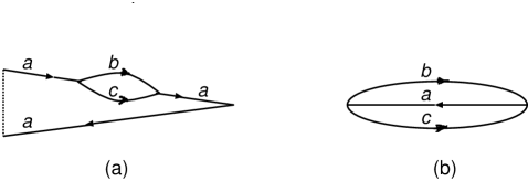
Figure 2: The diagram representation of the radiative correction to the probability of $a\rightarrow a$ transition.

In the low density limit (14) can be written through the light-cone wavefunction $\Psi_{a}^{bc}$

$$\frac{d^{3}P}{dxd\mbox{{\bf q}}_{b}}=\frac{1}{(2\pi)^{2}}\int\!d\mbox{{\boldmath$\tau$}}d\mbox{{\boldmath$\tau$}}^{{}^{\prime}}\exp(-i\mbox{{\bf q}}_{b}\mbox{{\boldmath$\tau$}}^{{}^{\prime}})\Psi_{a}^{bc*}(x,\mbox{{\boldmath$\tau$}}-\mbox{{\boldmath$\tau$}}^{{}^{\prime}})T\sigma_{\bar{a}bc}(\mbox{{\boldmath$\tau$}}_{bc},\mbox{{\boldmath$\tau$}}_{ab})\Psi_{a}^{bc}(x,\mbox{{\boldmath$\tau$}})\,,$$ (16)

where $\mbox{{\boldmath$\tau$}}_{bc}=\mbox{{\boldmath$\tau$}}$, $\mbox{{\boldmath$\tau$}}_{ab}=-[(1-x)\mbox{{\boldmath$\tau$}}+x\mbox{{\boldmath$\tau$}}^{{}^{\prime}}]$, $T=\int dzn(z)$. This formula can be obtained from (14) taking advantage of the representation for $\Psi_{a}^{bc}$ through $K_{bc}^{0}$

$$\Psi_{a}^{bc}(x,\mbox{{\boldmath$\tau$}})=\frac{i\lambda}{4E_{a}\sqrt{\pi x(1-x)}}\int\limits_{-\infty}^{0}dzK_{bc}^{0}(\mbox{{\boldmath$\tau$}},0|0,z)$$

established in [7]. Being divided by $T$ (16) gives a convenient formula for the Bethe-Heitler cross section in terms of the light-cone wavefunction. It worth noting that (16) (and (10), (14) as well) is valid if one can neglect the transverse motion effects on the scale of the medium constituent size. This assumes that the typical value of $|z_{2}-z_{1}|$ in (10), (14), which can be regarded as the formation length associated with the $a\rightarrow bc$ transition at a given $\mbox{{\bf q}}_{b}$, $L_{f}(q_{b})$, is much larger than the size of the medium constituent. If the LPM effect is not very strong the $L_{f}(q_{b})$ can be estimated replacing $m_{b,c}^{2}$ by $m_{b,c}^{2}+\mbox{{\bf q}}_{b}^{2}$ in the above formula for $L_{f}$. Note that for $L_{f}(q_{b})\gg L$ the radiation rate can be written through $\Psi_{a}^{bc}$ for arbitrary target density. In this case the target acts as a single scattering center and (14) can be written in a form like (16) but with the product $T\sigma_{\bar{a}bc}$ being replaced by $2\left\{1-\exp\left[-\frac{1}{2}T\sigma_{\bar{a}bc}\right]\right\}\,.$ This representation generalizes the formula for the $p_{T}$-integrated spectrum derived in [13].

In general case one can estimate the radiation rate using the parametrizations $\sigma_{i\bar{i}}=C_{ii}\mbox{{\boldmath$\tau$}}_{i}^{2}$, $\sigma_{\bar{a}bc}=C_{ab}\mbox{{\boldmath$\tau$}}_{ab}^{2}+C_{bc}\mbox{{\boldmath$\tau$}}_{bc}^{2}+C_{ca}\mbox{{\boldmath$\tau$}}_{ca}^{2}$ (here $\mbox{{\boldmath$\tau$}}_{ca}=-(\mbox{{\boldmath$\tau$}}_{ab}+\mbox{{\boldmath$\tau$}}_{bc})$). Then the Hamiltonian (12) takes the oscillator form with the frequency $\Omega(z)=\frac{(1-i)}{\sqrt{2}}\left[\frac{n(z)C(x)}{E_{a}x(1-x)}\right]^{1/2}\,,$ where $C(x)=C_{ab}(1-x)^{2}+C_{bc}+C_{ca}x^{2}$. The Green’s function for the oscillator Hamiltonian with the $z$-dependent frequency can be written in the form

$$K_{osc}(\mbox{{\boldmath$\tau$}}_{2},z_{2}|\mbox{{\boldmath$\tau$}}_{1},z_{1})=\frac{\gamma(z_{1},z_{2})}{2\pi i}\exp\left\{i\left[\alpha(z_{1},z_{2})\mbox{{\boldmath$\tau$}}_{2}^{2}+\beta(z_{1},z_{2})\mbox{{\boldmath$\tau$}}_{1}^{2}-\gamma(z_{1},z_{2})\mbox{{\boldmath$\tau$}}_{1}\mbox{{\boldmath$\tau$}}_{2}\right]\right\}\,.$$ (17)

The functions $\alpha$, $\beta$ and $\gamma$ in (17) can be evaluated in the approach of Ref. [14]. Then we can integrate analytically over $\mbox{{\boldmath$\tau$}}_{b}$ in (10), and represent the radiation rate as

$$\frac{d^{3}P}{dxd\mbox{{\bf q}}_{b}}=\frac{1}{(2\pi)^{2}}\mbox{Re}\int\limits_{z_{1}<z_{2}}\!dz_{1}dz_{2}\,g\,\frac{\gamma(z_{1},z_{2})}{Q(z_{1},z_{2})}\exp\left[-\frac{i\mbox{{\bf q}}^{2}_{b}}{4Q(z_{1},z_{2})}+\frac{i(z_{1}-z_{2})}{L_{f}}\right]\,,$$ (18)

where the factor $Q(z_{1},z_{2})$ can be expressed through the parameters $C_{ij}$, functions $\alpha$, $\beta$, $\gamma$, and $n$. The formula for this factor is cumbersome to be presented here.

Consider now the case when the particle $a$ is produced in a medium or at finite distance from a target. Equation (10) holds in this case as well but now $z_{i}$ equals the coordinate of the production point. Given the representation (10) taking advantage of (13) one can obtain a formula similar to (14) but with $[\Phi_{a}-1]$ being replaced by $\Phi_{a}$ in the second term. Note, however, that, due to infinite time required for the formation of $\Psi_{a}^{bc}$, equation (16) (and its analogue for arbitrary density at $L_{f}(q_{b})\gg L$) does not hold in this case.

Let us discuss briefly the totally inclusive radiation rate. It can be evaluated almost in the same way as the $\mbox{{\bf q}}_{c}$-integrated spectrum if one of the final particles has a zero charge, as this occurs for the $e\rightarrow\gamma e$ transition in QED. Consider the case when $e_{c}=0$. Since the particle $c$ does not interact with the medium the graph of Fig. 1a can be transformed into a graph like that of Fig. 1b but with the propagator $K_{c}$ being connected to the lower $abc$ vertex through the density matrix of the particle $c$. The corresponding formula (which is the analogue of (10)) reads

$$\frac{d^{5}P}{dxd\mbox{{\bf q}}_{b}d\mbox{{\bf q}}_{c}}=\frac{2}{(2\pi)^{2}}\mbox{Re}\int\!d\mbox{{\boldmath$\tau$}}_{b}d\mbox{{\boldmath$\tau$}}_{c}\,\exp\left[-i(\mbox{{\bf q}}_{b}\mbox{{\boldmath$\tau$}}_{b}+\mbox{{\bf q}}_{c}\mbox{{\boldmath$\tau$}}_{c})\right]$$

$$\times\int\limits_{z_{i}}^{z_{f}}\!dz_{1}\int\limits_{z_{1}}^{z_{f}}\!dz_{2}\,g\Phi_{b}(\mbox{{\boldmath$\tau$}}_{b},z_{2})K_{bc}(\mbox{{\boldmath$\tau$}}_{b}-\mbox{{\boldmath$\tau$}}_{c},z_{2}|0,z_{1})\Phi_{a}(\mbox{{\boldmath$\tau$}}_{a},z_{1})\,,$$ (19)

where $\mbox{{\boldmath$\tau$}}_{a}=x\mbox{{\boldmath$\tau$}}_{b}+(1-x)\mbox{{\boldmath$\tau$}}_{c}$. The $z$-integration in (19) can also be written as in (14). In the low density limit and at $L_{f}(q_{b})\gg L$ the initial- and final-state interaction vanish. For this reason the analogue of (16) and a similar equation for arbitrary density at $L_{f}(q_{b})\gg L$ which can be obtained from (19) are valid even when all the particles are charged.

The generalization of the above results to the realistic QED and QCD Lagrangians reduces to trivial replacements of the two- and three-body cross sections, and vertex factor $g$. The latter, due to spin effects in the vertex $a\rightarrow bc$, becomes an operator. The corresponding formulas are given in [6, 15].

The formalism developed can be applied to many problems. In particular, in QCD this approach can be used for evaluation of high-$p_{T}$ hadron spectra, the $p_{T}$-dependence of Drell-Yan pairs and heavy quarks production in $hA$-collisions, angular dependence of the parton energy loss in hot QCD matter produced in $AA$-collisions. It is also of interest for study the initial condition for quark-gluon plasma in $AA$-collisions. Some of these problems will be discussed in further publications.

I would like to thank N.N. Nikolaev and D. Schiff for discussions. I am grateful to J. Speth for the hospitality at FZJ, Jülich, where this work was completed. This work was partially supported by the grants INTAS 96-0597 and DFG 436RUS17/11/99.

References

• [1] L.D. Landau and I.Ya. Pomeranchuk, Dokl. Akad. Nauk SSSR 92, 535, 735 (1953).
• [2] A.B. Migdal, Phys. Rev. 103, 1811 (1956).
• [3] R. Baier, Yu.L. Dokshitzer, S. Peigne and D. Schiff, Phys. Lett. B345, 277 (1995).
• [4] J. Knoll and D.N. Voskresenskii, Phys. Lett. B351, 43 (1995).
• [5] R. Blankenbecler and S.D. Drell, Phys. Rev. D53, 6265 (1996); R. Blankenbecler, Phys. Rev. D55, 190 (1997).
• [6] B.G. Zakharov, JETP Lett. 63, 952 (1996).
• [7] B.G. Zakharov, JETP Lett. 64, 781 (1996).
• [8] R. Baier, Yu.L. Dokshitzer, A.H. Mueller, S. Peigne and D. Schiff, Nucl. Phys. B483, 291 (1997); B484, 265 (1997).
• [9] B.G. Zakharov, JETP Lett. 65, 615 (1997); hep-ph/9807396 (1998); hep-ph/9805271 (1998).
• [10] R. Baier, Yu.L. Dokshitzer, A.H. Mueller, and D. Schiff, Nucl. Phys. B531, 403 (1998); Phys. Rev. C58, 1706 (1998).
• [11] S.R. Klein, hep-ph/9802442 (1998).
• [12] B.G. Zakharov, Sov. J.Nucl. Phys. 46, 92 (1987).
• [13] N.N. Nikolaev, G. Piller, and B.G. Zakharov, JETP 81, 851 (1995).
• [14] B.Z. Kopeliovich and B.G. Zakharov, Phys. Rev. D44, 3466 (1991).
• [15] B.G. Zakharov, Phys. Atom. Nucl. 61, 838 (1998).