Yukawa Unification on the Bilinear R-Parity model

Abstract:

We discuss gauge and Yukawa unification in the context of a supersymmetric model with bilinear R–parity violation. We show that this model allows $b-\tau$ Yukawa unification for any value of $\tan\beta$ while satisfying perturbativity of the couplings. We also find the $t-b-\tau$ Yukawa unification easier to achieve than in the MSSM, occurring in a wider high $\tan\beta$ region. Finaly, we also discuss the compatibility between the predicted and the measured values for $\alpha_{s}(M_{Z})$.

1 Introduction

The Standard Model (SM) of particle physics is very successful in describing the interactions of the elementary particles, except possibly neutrinos. Although it is regarded as a good low-energy effective theory, the SM has many theoretical problems. Its gauge symmetry group is the direct product of three groups $SU(3)\times SU(2)\times U(1)$ and the corresponding gauge couplings are unrelated. It does not explain the three family structure of quarks and leptons, and their masses are fixed by arbitrary Yukawa couplings, with neutrinos being prevented from having mass. The Higgs sector, responsible for the symmetry breaking and for the fermion masses, has not been tested experimentally and the mass of the Higgs boson is unstable under radiative corrections.

In supersymmetry (SUSY) [1] the Higgs boson mass is stabilized under radiative corrections because the loops containing standard particles are partially canceled by the contributions from loops containing SUSY particles. If to the Minimal Supersymmetric Standard Model (MSSM) [2] we add the notion of Grand Unified Theory (GUT), then we find that the three gauge couplings approximately unify at a certain scale $M_{GUT}$ [3]. Indeed, measurements of the gauge couplings at the CERN $e^{+}e^{-}$ collider LEP and neutral current data [4] are in much better agreement with the MSSM–GUT with the SUSY scale $M_{SUSY}\raise 1.29167pt\hbox{$\;<$\kern-7.5pt\raise-4.73611pt\hbox{$\sim\;$}}1$ TeV [5], as compared with the SM.

Besides achieving gauge coupling unification [6], GUT theories also reduce the number of free parameters in the Yukawa sector. For example, in $SU(5)$ models, the bottom quark and the tau lepton Yukawa couplings are equal at the unification scale, and the predicted ratio $m_{b}/m_{\tau}$ at the weak scale agrees with experiments. Furthermore, a relation between the top quark mass and $\tan\beta=v_{u}/v_{d}$, the ratio between the vacuum expectation values of the two Higgs doublets is predicted. Two solutions are possible, characterized by low and high values of $\tan\beta$ [7]. In models with larger groups, such as $SO(10)$ and $E_{6}$, both the top and bottom Yukawa couplings are unified with the tau Yukawa at the unification scale [8]. In this case, only the large $\tan\beta$ solution survives.

In this talk we describe some recent results [9], that show that the minimal extension of the MSSM–GUT [10] in which R–Parity Violation (RPV) is introduced via a bilinear term in the MSSM superpotential [11, 12], allows $b$-$\tau$ Yukawa unification for any value of $\tan\beta$. We also analyze the $t$-$b$-$\tau$ Yukawa unification and find that it is easier to achieve than in the MSSM, occurring in a slightly wider high $\tan\beta$ region. We also address the question of the compatibility between the predicted and measured value for $\alpha_{s}(M_{Z})$ in the MSSM and in the bilinear RPV model.

2 Description of the Model

The superpotential $W$ is given by [11, 12]

$$W \hskip-2.84526pt=\hskip-2.84526pt \varepsilon_{ab}\!\left[h_{U}^{ij}\widehat{Q}_{i}^{a}\widehat{U}_{j}\widehat{H}_{u}^{b}\!+\!h_{D}^{ij}\widehat{Q}_{i}^{b}\widehat{D}_{j}\widehat{H}_{d}^{a}\!+\!h_{E}^{ij}\widehat{L}_{i}^{b}\widehat{R}_{j}\widehat{H}_{d}^{a}\right.$$ (2)

$$\left.\hskip 28.45274pt-\mu\widehat{H}_{d}^{a}\widehat{H}_{u}^{b}+\epsilon_{i}\widehat{L}_{i}^{a}\widehat{H}_{u}^{b}\right]$$

where $i,j=1,2,3$ are generation indices, $a,b=1,2$ are $SU(2)$ indices. This superpotential is motivated by models of spontaneous breaking of R–Parity [13]. Here R–Parity and lepton number are explicitly violated by the last term in Eq. (2).

The set of soft SUSY breaking terms are

$$V_{soft} \hskip-2.84526pt=\hskip-2.84526pt M_{Q}^{ij2}\widetilde{Q}^{a*}_{i}\widetilde{Q}^{a}_{j}+M_{U}^{ij2}\widetilde{U}^{*}_{i}\widetilde{U}_{j}+M_{D}^{ij2}\widetilde{D}^{*}_{i}\widetilde{D}_{j}$$ (7)

$$\hskip-14.22636pt+M_{L}^{ij2}\widetilde{L}^{a*}_{i}\widetilde{L}^{a}_{j}+M_{R}^{ij2}\widetilde{R}^{*}_{i}\widetilde{R}_{j}+m_{H_{d}}^{2}H^{a*}_{d}H^{a}_{d}$$

$$\hskip-14.22636pt+m_{H_{u}}^{2}H^{a*}_{u}H^{a}_{u}-\left[{\textstyle{1\over 2}}\sum M_{i}\lambda_{i}\lambda_{i}+h.c.\right]$$

$$\hskip-14.22636pt+\varepsilon_{ab}\left[A_{U}^{ij}\widetilde{Q}^{a}_{i}\widetilde{U}_{j}H_{u}^{b}+A_{D}^{ij}\widetilde{Q}^{b}_{i}\widetilde{D}_{j}H_{d}^{a}\right.$$

$$\hskip-14.22636pt\left.+A_{E}^{ij}\widetilde{L}^{b}_{i}\widetilde{R}_{j}H_{d}^{a}\!-\!B\mu H_{d}^{a}H_{u}^{b}\!+\!B_{i}\epsilon_{i}\widetilde{L}^{a}_{i}H_{u}^{b}\right]\,.$$

The bilinear R-parity violating term cannot be eliminated by superfield redefinition. The reason [14] is that the bottom Yukawa coupling, usually neglected, plays a crucial role in splitting the soft-breaking parameters $B$ and $B_{i}$ as well as the scalar masses $m_{H_{d}}^{2}$ and $M_{L}^{2}$, assumed to be equal at the unification scale.

The electroweak symmetry is broken when the VEVS of the two Higgs doublets $H_{d}$ and $H_{u}$, and the sneutrinos.

$$H_{d} = {{{1\over{\sqrt{2}}}[\chi^{0}_{d}+v_{d}+i\varphi^{0}_{d}]}\choose{H^{-}_{d}}}$$ (8)

$$H_{u} = {{H^{+}_{u}}\choose{{1\over{\sqrt{2}}}[\chi^{0}_{u}+v_{u}+i\varphi^{0}_{u}]}}$$ (9)

$$L_{i} = {{{1\over{\sqrt{2}}}[\tilde{\nu}^{R}_{i}+v_{i}+i\tilde{\nu}^{I}_{i}]}\choose{\tilde{\ell}^{i}}}$$ (10)

The gauge bosons $W$ and $Z$ acquire masses

$$m_{W}^{2}={\textstyle{1\over 4}}g^{2}v^{2}\quad;\quad m_{Z}^{2}={\textstyle{1\over 4}}(g^{2}+g^{\prime 2})v^{2}$$ (11)

where

$$v^{2}\equiv v_{d}^{2}+v_{u}^{2}+v_{1}^{2}+v_{2}^{2}+v_{3}^{2}=(246\;{\rm GeV})^{2}$$ (12)

We introduce the following notation in spherical coordinates:

$$v_{d} = v\sin\theta_{1}\sin\theta_{2}\sin\theta_{3}\cos\beta$$ (13)

$$v_{u} = v\sin\theta_{1}\sin\theta_{2}\sin\theta_{3}\sin\beta$$ (14)

$$v_{1} = v\sin\theta_{1}\sin\theta_{2}\cos\theta_{3}$$ (15)

$$v_{2} = v\sin\theta_{1}\cos\theta_{2}$$ (16)

$$v_{3} = v\cos\theta_{1}$$

which preserves the MSSM definition $\tan\beta=v_{u}/v_{d}$. The angles $\theta_{i}$ are equal to $\pi/2$ in the MSSM limit.

The full scalar potential may be written as

$$V_{total}=\sum_{i}\left|{\partial W\over\partial z_{i}}\right|^{2}+V_{D}+V_{soft}+V_{RC}$$ (17)

where $z_{i}$ denotes any one of the scalar fields in the theory, $V_{D}$ are the usual $D$-terms, $V_{soft}$ the SUSY soft breaking terms, and $V_{RC}$ are the one-loop radiative corrections.

In writing $V_{RC}$ we use the diagrammatic method and find the minimization conditions by correcting to one–loop the tadpole equations. This method has advantages with respect to the effective potential when we calculate the one–loop corrected scalar masses. The scalar potential contains linear terms,

$$V_{linear}=t_{d}\sigma^{0}_{d}+t_{u}\sigma^{0}_{u}+t_{i}\tilde{\nu}^{R}_{i}\equiv t_{\alpha}\sigma^{0}_{\alpha}\,,$$ (18)

where we have introduced the notation

$$\sigma^{0}_{\alpha}=(\sigma^{0}_{d},\sigma^{0}_{u},\nu^{R}_{1},\nu^{R}_{2},\nu^{R}_{3})$$ (19)

and $\alpha=d,u,1,2,3$. The one loop tadpoles are

$$t_{\alpha} = t^{0}_{\alpha}-\delta t^{\overline{MS}}_{\alpha}+T_{\alpha}(Q)$$ (20)

$$= t^{0}_{\alpha}+T^{\overline{MS}}_{\alpha}(Q)$$ (21)

where $T^{\overline{MS}}_{\alpha}(Q)\equiv-\delta t^{\overline{MS}}_{\alpha}+T_{\alpha}(Q)$ are the finite one–loop tadpoles.

In the following we will consider the one generation version of this model, where only $\epsilon_{3}\not=0$. Then $v_{1}=v_{2}=0$ if $\epsilon_{1}=\epsilon_{2}=0$.

3 Main Features

The $\epsilon$–model is a one(three) parameter(s) generalization of the MSSM. It can be thought as an effective model showing the more important features of the SBRP–model [13] at the weak scale. The mass matrices, charged and neutral currents, are similar to the SBRP–model if we identify

$$\epsilon\equiv v_{R}h_{\nu}$$ (22)

The R–Parity violating parameters $\epsilon_{3}$ and $v_{3}$ violate tau–lepton number, inducing a non-zero $\nu_{\tau}$ mass $m_{\nu_{\tau}}\propto(\mu v_{3}+\epsilon_{3}v_{d})^{2}$, which arises due to mixing between the weak eigenstate $\nu_{\tau}$ and the neutralinos. The $\nu_{e}$ and $\nu_{\mu}$ remain massless in first approximation. They acquire masses from supersymmetric loops [15, 16] that are typically smaller than the tree level mass.

The model has the MSSM as a limit. This can be illustrated in Figure 1 where we show the ratio of the lightest CP-even Higgs boson mass $m_{h}$ in the $\epsilon$–model and in the MSSM as a function of $v_{3}$. Many other results concerning this model and the implications for physics at the accelerators can be found in ref. [11, 12].

Figure 1: Ratio of the lightest CP-even Higgs boson mass $m_{h}$ in the $\epsilon$–model and in the MSSM as a function of $v_{3}$.

4 Radiative Breaking

4.1 Radiative Breaking in the $\epsilon\!$ model: The minimal case

At $Q=M_{GUT}$ we assume the standard minimal supergravity unifications assumptions,

$$A_{t}=A_{b}=A_{\tau}\equiv A\>,$$ (23)

$$\vbox to24.0pt{}B=B_{2}=A-1\>,$$ (24)

$$\vbox to24.0pt{}m_{H_{1}}^{2}=m_{H_{2}}^{2}=M_{L}^{2}=M_{R}^{2}=m_{0}^{2}\>,$$ (25)

$$\vbox to24.0pt{}M_{Q}^{2}=M_{U}^{2}=M_{D}^{2}=m_{0}^{2}\>,$$ (26)

$$\vbox to24.0pt{}M_{3}=M_{2}=M_{1}=M_{1/2}$$ (27)

In order to determine the values of the Yukawa couplings and of the soft breaking scalar masses at low energies we first run the RGE’s from the unification scale $M_{GUT}\sim 10^{16}$ GeV down to the weak scale. We randomly give values at the unification scale for the parameters of the theory.

$$\begin{array}[]{ccccc}10^{-2}&\leq&{h^{2}_{t}}_{GUT}/4\pi&\leq&1\cr 10^{-5}&\leq&{h^{2}_{b}}_{GUT}/4\pi&\leq&1\cr-3&\leq&A/m_{0}&\leq&3\cr 0&\leq&\mu^{2}_{GUT}/m_{0}^{2}&\leq&10\cr 0&\leq&M_{1/2}/m_{0}&\leq&5\cr 10^{-2}&\leq&{\epsilon^{2}_{3}}_{GUT}/m_{0}^{2}&\leq&10\cr\end{array}$$ (28)

The value of ${h^{2}_{\tau}}_{GUT}/4\pi$ is defined in such a way that we get the $\tau$ lepton mass correctly. As the charginos mix with the tau lepton, through a mass matrix is given by

$${\bf M_{C}}=\left[\matrix{M&{\textstyle{1\over{\sqrt{2}}}}gv_{u}&0\cr{\textstyle{1\over{\sqrt{2}}}}gv_{d}&\mu&-{\textstyle{1\over{\sqrt{2}}}}h_{\tau}v_{3}\cr{\textstyle{1\over{\sqrt{2}}}}gv_{3}&-\epsilon_{3}&{\textstyle{1\over{\sqrt{2}}}}h_{\tau}v_{d}}\right]$$

Imposing that one of the eigenvalues reproduces the observed tau mass $m_{\tau}$, $h_{\tau}$ can be solved exactly as [12]

$$h_{\tau}^{2}={{2m_{\tau}^{2}}\over{v_{d}}}\left[{{1+\delta_{1}}\over{1+\delta_{2}}}\right]$$

where the $\delta_{i}\,$, $i=1,2$, depend on $m_{\tau}$, on the SUSY parameters $M,\mu,\tan\beta$ and on the R-Parity violating parameters $\epsilon_{3}$ and $v_{3}$. It can be shown [12] that

$$\lim_{\epsilon_{3}\rightarrow 0}\delta_{i}=0$$ (29)

After running the RGE we have a complete set of parameters, Yukawa couplings and soft-breaking masses $m^{2}_{i}(RGE)$ to study the minimization. To do this we use the following method [10]:

1. We start with random values for $h_{t}$ and $h_{b}$ at $M_{GUT}$. The value of $h_{\tau}$ at $M_{GUT}$ is fixed in order to get the correct $\tau$ mass.

2. The value of $v_{d}$ is determined from $m_{b}=h_{b}v_{d}/\sqrt{2}$ for $m_{b}=2.8$ GeV (running $b$ mass at $m_{Z}$).

3. The value of $v_{u}$ is determined from $m_{t}=h_{t}v_{u}/\sqrt{2}$ for $m_{t}=176\pm 5$ GeV. If

   $$\hskip-1.42262ptv_{d}^{2}+v_{u}^{2}\!>\!v^{2}=\frac{4}{g^{2}}\,m^{2}_{W}=(246\hbox{ GeV})^{2}$$ (30)

   then we go back and choose another starting point. The value of $v_{3}$ is then obtained from

   $$v_{3}=\pm\,\sqrt{\frac{4}{g^{2}}\,m^{2}_{W}-v_{1}^{2}-v_{2}^{2}}$$ (31)

We see that the freedom in $h_{t}$ and $h_{b}$ at $M_{GUT}$ can be translated into the freedom in the mixing angles $\beta$ and $\theta$. Comparing, at this point, with the MSSM we have one extra parameter $\theta$. We will discuss this in more detail below. In the MSSM we would have $\theta=\pi/2$. After doing this, for each point in parameter space, we solve the extremum equations, for the soft breaking masses, which we now call $m^{2}_{i}$ ($i=H_{1},H_{2},L$). Then we calculate numerically the eigenvalues for the real and imaginary part of the neutral scalar mass-squared matrix. If they are all positive, except for the Goldstone boson, the point is a good one. If not, we go back to the next random value. As before, we end up with a set of solutions for which the $m^{2}_{i}$ obtained from the minimization of the potential differ from those obtained from the RGE, which we call $m^{2}_{i}(RGE)$. Our goal is to find solutions that obey

$$m^{2}_{i}=m^{2}_{i}(RGE)\quad\forall i$$ (32)

To do that we define a function

$$\eta=max\left(\frac{m^{2}_{i}}{m^{2}_{i}(RGE)},\frac{m^{2}_{i}(RGE)}{m^{2}_{i}}\right)\quad\forall i$$ (33)

We see that we have always

$$\eta\geq 1$$ (34)

and use MINUIT to minimize $\eta$. We have shown [10] that it is easy to get solutions for this problem.

Before we finish this section let us discuss the counting of free parameters. In the minimal N=1 supergravity unified version of the MSSM this is shown in Table 1. The counting for the $\epsilon$–model is presented in Table 2. Finally, we note that in either case, the sign of the mixing parameter $\mu$ is physical and has to be taken into account.

Parameters	Conditions	Free Parameters
$h_{t}$, $h_{b}$, $h_{\tau}$	$m_{W}$, $m_{t}$	$\tan\beta$
$v_{d}$, $v_{u}$,$M_{1/2}$	$m_{b}$, $m_{\tau}$	2 Extra
$m_{0}$, $A$, $\mu$	$t_{i}=0$, $i=1,2$	(e.g. $m_{h}$, $m_{A}$)
Total = 9	Total = 6	Total = 3

Table 1: Counting of free parameters in N=1 supergravity MSSM.

Parameters	Conditions	Free Parameters
$h_{t}$, $h_{b}$, $h_{\tau}$	$m_{W}$, $m_{t}$	$\tan\beta$, $\epsilon_{i}$
$v_{d}$, $v_{u}$, $M_{1/2}$	$m_{b}$, $m_{\tau}$
$m_{0}$,$A$, $\mu$	$t_{i}=0$	2 Extra
$v_{i}$, $\epsilon_{i}$	($i=1,\ldots,5$)	(e.g. $m_{h}$, $m_{A}$)
Total = 15	Total = 9	Total = 6

Table 2: Counting of free parameters in our model.

4.2 Yukawa Unification in the $\epsilon$ model: I Motivation

There is a strong motivation to consider GUT theories where both gauge and Yukawa unification can achieved. This is because besides achieving gauge coupling unification, GUT theories can also reduce the number of free parameters in the Yukawa sector and this is normally a desirable feature. The situation with respect to GUT theories that embed the MSSM can be summarized as follows [7, 8]:

• In $SU(5)$ models, $h_{b}=h_{\tau}$ at $M_{GUT}$. The predicted ratio $m_{b}/m_{\tau}$ at $M_{WEAK}$ agrees with experiments.

• A relation between $m_{top}$ and $\tan\beta$ is predicted. Two solutions are possible: low and high $\tan\beta$ .

• In $SO(10)$ and $E_{6}$ models $h_{t}=h_{b}=h_{\tau}$ at $M_{GUT}$. In this case, only the large $\tan\beta$ solution survives.

• Recent global fits of low energy data (the lightest Higgs mass and $B(b\rightarrow s\gamma)$) to MSSM show that it is hard to reconcile these constraints with the large $\tan\beta$ solution. Also the low $\tan\beta$ solution with $\mu<0$ is also disfavored.

In the following sections we will show [9] that the $\epsilon$–model allows $b-\tau$ Yukawa unification for any value of $\tan\beta$ and satisfying perturbativity of the couplings. We also find the $t-b-\tau$ Yukawa unification easier to achieve than in the MSSM, occurring in a wider high $\tan\beta$ region.

4.3 Yukawa Unification in the $\epsilon$ model: II The Method

As before $h_{\tau}$ can be solved exactly

$$h_{\tau}^{2}={{2m_{\tau}^{2}}\over{v_{d}}}\left[{{1+\delta_{1}}\over{1+\delta_{2}}}\right]$$ (35)

where the $\delta_{i}\,$, $i=1,2$, depend on $m_{\tau}$, on the SUSY parameters $M,\mu,\tan\!\beta$ and on the R-parity violating parameters $\epsilon_{3}$ and $v_{3}$. Also $h_{t}$ and $h_{b}$ are related to $m_{t}$ and $m_{b}$

$$m_{t}=h_{t}\frac{v}{\sqrt{2}}\sin\beta\sin\theta\,,\>\>\>\>\>m_{b}=h_{b}\frac{v}{\sqrt{2}}\cos\beta\sin\theta$$ (36)

where

$$v=2m_{W}/g\ ;\ \tan\beta=v_{u}/v_{d}\ ;\ \cos\theta=v_{3}/v$$ (37)

In our approach we divide the evolution in three ranges:

1. $m_{Z}\rightarrow m_{t}$
   We use running fermion masses and gauge couplings.

2. $m_{t}\rightarrow M_{SUSY}$
   We use the two-loop SM RGE’s including the quartic Higgs coupling $\lambda$.

3. $M_{SUSY}\rightarrow M_{GUT}$
   We use the two-loop RGE’s.

Using a top $\rightarrow$ bottom approach we randomly vary the unification scale $M_{GUT}$ and the unified coupling $\alpha_{GUT}$ looking for solutions compatible with the low energy data [17]

$$\alpha^{-1}_{em}(m_{Z})=128.896\pm 0.090$$ (38)

$$\vbox to18.0pt{}\sin^{2}\theta_{w}(m_{Z})=0.2322\pm 0.0010$$ (39)

$$\vbox to18.0pt{}\alpha_{s}(m_{Z})=0.118\pm 0.003$$ (40)

We get a region centered around

$$M_{GUT}\approx 2.3\times 10^{16}GeV\ ;\ {\alpha_{GUT}}^{-1}\approx 24.5$$ (41)

Next we use a bottom $\rightarrow$ top approach to study the unification of Yukawa couplings using two-loop RGEs. We take [17]

$$m_{W}=80.41\pm 0.09\ GeV$$ (42)

$$\vbox to18.0pt{}m_{\tau}=1777.0\pm 0.3\ MeV$$ (43)

$$\vbox to18.0pt{}m_{b}(m_{b})=4.1\ \hbox{to}\ 4.5\ GeV$$ (44)

We calculate the running masses

$$m_{\tau}(m_{t}) = \eta_{\tau}^{-1}m_{\tau}(m_{\tau})$$ (45)

$$\vbox to18.0pt{}m_{b}(m_{t}) = \eta_{b}^{-1}m_{b}(m_{b})$$ (46)

where $\eta_{\tau}$ and $\eta_{b}$ include three–loop order QCD and one–loop order QED [18]. At the scale $Q=m_{t}$ we keep as a free parameter the running top quark mass $m_{t}(m_{t})$ and vary randomly the SM quartic Higgs coupling $\lambda$. In solving the RG equations we take the following boundary conditions:

1. At scale $Q=m_{t}$

   $$\lambda_{i}^{2}(m_{t})=2m_{i}^{2}(m_{t})/v^{2}\ ;\ i=t,b,\tau$$ (47)

2. At scale $Q=M_{SUSY}$

   $$\lambda_{t}(M_{SUSY}^{-}) = h_{t}(M_{SUSY}^{+})\sin\beta\sin\theta$$ (48)

   $$\vbox to18.0pt{}\lambda_{b}(M_{SUSY}^{-}) = h_{b}(M_{SUSY}^{+})\cos\beta\sin\theta$$ (49)

   $$\vbox to18.0pt{}\lambda_{\tau}(M_{SUSY}^{-}) = h_{\tau}(M_{SUSY}^{+})\cos\beta\sin\theta$$ (51)

   $$\vbox to20.0pt{}\times\sqrt{{1+\delta_{2}}\over{1+\delta_{1}}}$$

   where $h_{i}$ denote the Yukawa couplings of our model and $\lambda_{i}$ those of the SM. The boundary condition for the quartic Higgs coupling is

   $$\lambda(M_{SUSY}^{-}) \hskip-5.69054pt=\hskip-5.69054pt {\textstyle{1\over 4}}\!\Big{[}(g^{2}(M_{SUSY}^{+})\!+\!g^{\prime 2}(M_{SUSY}^{+})\Big{]}$$ (53)

   $$\vbox to18.0pt{}(\cos 2\beta\sin^{2}\theta+\cos^{2}\theta)^{2}$$

   The MSSM limit is obtained setting $\theta\to\pi/2$ i.e. $v_{3}=0$.

Before we close this section we give some details of the calculation. At the scale $Q=M_{SUSY}$ we vary randomly the SUSY parameters $M$, $\mu$ and $\tan\beta$, as well as the R–Parity violating parameter $\epsilon_{3}$. The parameter $v_{3}=v\cos\theta$ is calculated from the boundary conditions. Since $\lambda$ (or equivalently the SM Higgs mass $m_{H}^{2}=2\lambda v^{2}$) is varied randomly, in practice we also scan over $\theta$. This way, we consider all possible initial conditions for the RGEs at $Q=M_{SUSY}$, and evolve them up to the unification scale $Q=M_{GUT}$. The solutions that satisfy $b-\tau$ unification are kept.

4.4 Yukawa Unification in the $\epsilon$ model: III Results and Discussion

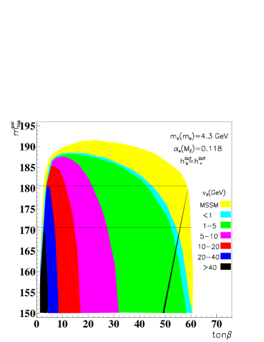
Figure 2: Top quark mass as a function of $\tan\beta$ for different values of the R–Parity violating parameter $v_{3}$. Bottom quark and tau lepton Yukawa couplings are unified at $M_{GUT}$. The horizontal lines correspond to the $1\sigma$ experimental $m_{t}$ determination. Points with $t-b-\tau$ unification lie in the diagonal band at high $\tan\beta$ values. We have taken $M_{SUSY}=m_{t}$.

The results are summarized in Figure 2 where we present the top quark mass as a function of $\tan\beta$ for different values of the R–Parity violating parameter $v_{3}$. Bottom quark and tau lepton Yukawa couplings are unified at $M_{GUT}$. The horizontal lines correspond to the $1\sigma$ experimental $m_{t}$ determination. Points with $t-b-\tau$ unification lie in the diagonal band at high $\tan\beta$ values. We have taken $M_{SUSY}=m_{t}$. The dependence of our results on $\alpha_{s}$ and $m_{b}$ is totally analogous to what happens in the MSSM. The upper bound on $\tan\beta$, which is $\tan\beta\raise 1.29167pt\hbox{$\;<$\kern-7.5pt\raise-4.73611pt\hbox{$\sim\;$}}61$ for $\alpha_{s}=0.118$, increases with $\alpha_{s}$ and becomes $\tan\beta\raise 1.29167pt\hbox{$\;<$\kern-7.5pt\raise-4.73611pt\hbox{$\sim\;$}}63$ (59) for $\alpha_{s}=0.122$ (0.114). The top mass value for which unification is achieved for any $\tan\beta$ value within the perturbative region increases with $\alpha_{s}$, as in the MSSM. As for the dependence on $m_{b}$, if we consider $m_{b}(m_{b})=4.1$ (4.5) GeV then the upper bound of this parameter is given by $\tan\beta\raise 1.29167pt\hbox{$\;<$\kern-7.5pt\raise-4.73611pt\hbox{$\sim\;$}}64$ (58). In addition, the MSSM region is narrower (wider) at high $\tan\beta$ compared with the $m_{b}(m_{b})=4.3$ GeV case. The line at high $\tan\beta$ values corresponds to points where $t-b-\tau$ unification is achieved. Since the region with $|v_{3}|<5$ GeV overlaps with the MSSM region, it follows that $t-b-\tau$ unification is possible in this model for values of $|v_{3}|$ up to about 5 GeV, instead of 50 GeV or so, which holds in the case of bottom-tau unification.

5 On $\alpha_{3}(M_{Z})$ versus $\sin^{2}\theta_{W}(M_{Z})$

Recent studies [19] of gauge coupling unification in the context of minimal R–Parity conserving supergravity (SUGRA) agree that using the experimental values for the electromagnetic coupling and the weak mixing angle, the prediction obtained for $\alpha_{s}(M_{Z})\sim 0.129\pm 0.010$ is about 2$\sigma$ larger than indicated by the most recent world average value $\alpha_{s}(M_{Z})^{W.A}=0.1189\pm 0.0015$ [20].

We have re-considered the $\alpha_{s}$ prediction in the context of the model with bilinear breaking of R–Parity. We have shown [21], that in this simplest SUGRA R–Parity breaking model, with the same particle content as the MSSM, there appears an additional negative contribution to $\alpha_{s}$, which can bring the theoretical prediction closer to the experimental world average. This additional contribution comes from two–loop b–quark Yukawa effects on the renormalization group equations for $\alpha_{s}$. Moreover we have shown that this contribution is typically correlated to the tau–neutrino mass which is induced by R–Parity breaking and which controls the R-Parity violating effects. We found that it is possible to get a 5% effect on $\alpha_{s}(M_{Z})$ even for light $\nu_{\tau}$ masses. The results are summarized in Figure 3 where we present the situation for the MSSM and in Figure 4 where the results for the bilinear R–Parity breaking model are shown.

Figure 3: $\alpha_{s}(M_{Z})$ versus $\hat{s}_{Z}$ for the MSSM.

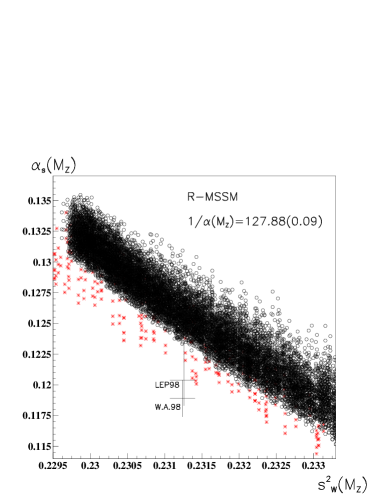
Figure 4: $\alpha_{s}(M_{Z})$ versus $\hat{s}_{Z}$ for the bilinear $\not{\!\!\!\!R}_{p}$ model.

6 Conclusions

The bilinear R–Parity model is a minimal extension of the MSSM with many new features, among which the possibility of having masses for the neutrinos. We have shown that it is possible to incorporate these models in a N=1 SUGRA scenario, where the number of free parameters is reduced. In these so–called radiative breaking scenarios we showed that this model allows $b-\tau$ Yukawa unification for any value of $\tan\beta$ while satisfying perturbativity of the couplings. We also find the $t-b-\tau$ Yukawa unification easier to achieve than in the MSSM, occurring in a wider high $\tan\beta$ region. By performing a full two–loop calculation [21] we also have shown that in this model there appears an additional negative contribution to $\alpha_{s}$, which can bring the theoretical prediction closer to the experimental world average. Although we presented here only the one generation example, we have achieved also the above results in the full three generation case. In this situation we can get at one–loop non zero values for the masses of the two lightest neutrinos which very interesting in the context of solving the solar and atmospheric neutrino problems [16].

References

- [1] Yu.A. Gol’fand and E.P. Likhtman, Sov. Phys. JETP Lett. 13 (1971) 323; D.V. Volkov and V.P. Akulov, Sov. Phys. JETP Lett. 16 (1972) 438; J. Wess and B. Zumino, Nucl. Phys. B 70 (1974) 39.
- [2] H.P. Nilles, Phys. Rept. 110 (1984) 1; H.E. Haber and G.L. Kane, Phys. Rept. 117 (1985) 75; R. Barbieri, Riv. Nuovo Cimento 11 (1988) 1.
- [3] S. Dimopoulos, S. Raby, and F. Wilczek, Phys. Rev. D 24 (1981) 1681; S. Dimopoulos and H. Georgi, Nucl. Phys. B 193 (1981) 150; L. Ibañez and G.G. Ross, Phys. Lett. B 105 (1981) 439; M.B. Einhorn and D.R.T. Jones, Nucl. Phys. B 196 (1982) 475; W.J. Marciano and G. Senjanovic, Phys. Rev. D 25 (1982) 3092.
- [4] Review of Particle Properties, Phys. Rev. D 54 (1996) 1.
- [5] U. Amaldi, W. de Boer, and H. Furstenau, Phys. Lett. B 260 (1991) 447; J. Ellis, S. Kelley, and D.V. Nanopoulos, Phys. Lett. B 260 (1991) 131; P. Langacker and M. Luo, Phys. Rev. D 44 (1991) 817; C. Giunti, C.W. Kim and U.W. Lee, Mod. Phys. Lett. A 6 (1991) 1745.
- [6] For recent studies see P. Langacker and N. Polonsky, Phys. Rev. D 47 (1993) 4028; P.H. Chankowski, Z. Pluciennik, and S. Pokorski, Nucl. Phys. B 439 (1995) 23; P.H. Chankowski, Z. Pluciennik, S. Pokorski, and C.E. Vayonakis, Phys. Lett. B 358 (1995) 264.
- [7] V. Barger, M.S. Berger, and P. Ohmann, Phys. Rev. D 47 (1993) 1093; M. Carena, S. Pokorski, and C.E.M. Wagner, Nucl. Phys. B 406 (1993) 59; R. Hempfling, Phys. Rev. D 49 (1994) 6168.
- [8] L.J. Hall, R. Rattazzi, and U. Sarid, Phys. Rev. D 50 (1994) 7048; M. Carena, M. Olechowski, S. Pokorski, and C.E.M. Wagner, Nucl. Phys. B 426 (1994) 269.
- [9] M.A. Díaz, J. Ferrandis, J.C. Romão, and J.W.F. Valle, Phys. Lett. B 453 (1999) 263.
- [10] M.A. Díaz, J.C. Romão, and J.W.F. Valle, Nucl. Phys. B 524 (1998) 23; M.A. Díaz, talk given at International Europhysics Conference on High-Energy Physics, Jerusalem, Israel, 19-26 Aug 1997, hep-ph/9712213; J.C. Romão, talk given at International Workshop on Physics Beyond the Standard Model: From Theory to Experiment (Valencia 97), Valencia, Spain, 13-17 Oct 1997, hep-ph/9712362; J.W.F. Valle, review talk given at the Workshop on Physics Beyond the Standard Model: Beyond the Desert: Accelerator and Nonaccelerator Approaches, Tegernsee, Germany, 8-14 Jun 1997, hep-ph/9712277.
- [11] F. de Campos, M.A. García-Jareño, A.S. Joshipura, J. Rosiek, and J. W. F. Valle, Nucl. Phys. B 451 (1995) 3;T. Banks, Y. Grossman, E. Nardi, and Y. Nir, Phys. Rev. D 52 (1995) 5319; A. S. Joshipura and M.Nowakowski, Phys. Rev. D 51 (1995) 2421; R. Hempfling, Nucl. Phys. B 478 (1996) 3; F. Vissani and A.Yu. Smirnov, Nucl. Phys. B 460 (1996) 37; H. P. Nilles and N. Polonsky, Nucl. Phys. B 484 (1997) 33; B. de Carlos, P. L. White, Phys. Rev. D 55 (1997) 4222; S. Roy and B. Mukhopadhyaya, Phys. Rev. D 55 (1997) 7020.
- [12] A. Akeroyd, M.A. Díaz, J. Ferrandis, M.A. Garcia–Jareño, and J.W.F. Valle, Nucl. Phys. B 529 (1998) 3.
- [13] A. Masiero and J.W.F. Valle, Phys. Lett. B 251 (1990) 273; M.C. Gonzalez-Garcia, J.W.F. Valle, Nucl. Phys. B 355 (1991) 330; J.C. Romão, C.A. Santos, J.W.F. Valle, Phys. Lett. B 288 (1992) 311; J.C. Romão, A. Ioannissyan and J.W.F. Valle, Phys. Rev. D 55 (1997) 427.
- [14] M.A. Díaz, talk given at International Workshop on Physics Beyond the Standard Model: From Theory to Experiment (Valencia 97), Valencia, Spain, 13-17 Oct 1997, hep-ph/9802407.
- [15] R. Hempfling, Nucl. Phys. B 478 (1996) 3.
- [16] M.A. Díaz, M. Hirsch, W. Porod, J.C. Romão and J.W.F. Valle in preparation. See also J.C. Romão talk at the International Workshop on Particles in Astrophysics and Cosmology: From Theory to Observation, València, Spain, 3-8 May 1999.
- [17] “A Combination of Preliminary Electroweak Measurements and Constraints on the Standard Model”, CERN internal note, LEPEWWG/97-02, Aug. 1997.
- [18] O. V. Tarasov, A. A. Vladimirov, and A. Y. Zharkov, Phys. Lett. B 93 (1980) 429; S.G. Gorishny, A.L. Kateav, and S.A. Larin, Yad. Fiz. 40 (1984) 517 [Sov. J. Nucl. Phys. 40 (1984) 329]; S.G. Gorishny et. al., Mod. Phys. Lett. A 5 (1990) 2703.
- [19] P. Langacker and N. Polonsky, Phys. Rev. D 47 (1993) 4028; P. Langacker and N. Polonsky, Phys. Rev. D 52 (1995) 3081; M. Carena, S. Pokorski and C.E.M. Wagner, Nucl. Phys. B 406 (1993) 59.
- [20] C. Caso et. al. Eur. Phys. J. C 3 (1998) 1.
- [21] M.A.Díaz, J. Ferrandis, J.C. Romão and J.W.F. Valle, hep-ph/9906343.