hep-ph/9906517

Supersymmetric radiative corrections to top quark and Higgs boson physics

Jaume Guasch Inglada

Universitat Autònoma de Barcelona

Grup de Física Teòrica

Institut de Física d’Altes Energies

Memòria presentada com a Tesi Doctoral per a optar al títol de Doctor en Física per la Universitat Autònoma de Barcelona.

Aquesta memòria és la tesi doctoral

“Supersymmetric radiative corrections to top quark and Higgs boson physics”

Fou realitzada per en

Jaume Guasch Inglada

sota la direcció del

Dr. Joan Solà i Peracaula

professor titular de Física Teòrica de la Facultat de Ciències de la Universitat Autònoma de Barcelona.

Va ser llegida el dia 18 de gener de 1999 a la sala de seminaris de l’IFAE de la Universitat Autònoma de Barcelona.

Tesi publicada per la Universitat Autònoma de Barcelona amb ISBN 84-490-1544-8

Podriem dir que aquesta tesi és bàsicament filla meva, però les criatures també ténen un avi, sense el qual mai haurien pogut arribar a nèixer, en aquest cas l’avi és en Joan Solà. Des d’un primer moment (i fins a l’ultim minut!) hem treballat dur. Quan sorgeix algun problema imprevist, sempre hi sol haver alguna carpeta d’apunts que ens simplifica la vida. A partir de la teva tesi hem pogut anar desgranant els camins cap a nous mons. He tingut la oportunitat de treballar, ben encarrilat, però amb força llibertat. Gràcies per haver tingut la oportunitat de treballar amb tu.

Les criatures mai van soles, si no estan acompanyades de canalla de la mateixa edat (any més, any menys) els falta alguna cosa, i als pares també! aquesta tesi ha anat creixent al costat d’altres, amb col$\cdot$laboracions, cafès, subrutines FORTRAN agafades, deixades, robades …, codi Mathematica i LaTeX  amunt i avall, discussions (de física i, sobretot, d’altres coses), acudits, …, més d’un ensurt (on c… defineixes la massa del bottom!!!, H… no ho sé!!), que, afortunadament, gairebé sempre s’acaben en res (ufff! és al common Other_Standard_Model_Masses_new_2), tot això gràcies al companys meravellosos del SUSY Team de l’IFAE, en David, en Ricard i en Toni, si els hagués d’agrair tot el que m’han ajudat (començant pels inicis difícils amb els ordinadors, i acabant per nombrosos suggeriments i correccions) no cabrien en aquesta plana.

A la física no tot es SUSY, hi ha també reticles, bombolletes a l’univers, etc., i gràcies a aquestes coses hi ha companys de doctorat que entre cafès, sopars, i costellades, ens ajuden a pujar la moral.

Gracies també als membres del Grup de Física Teòrica de l’U.A.B. per haver-me ofert la possibilitat de realitzar-hi el doctorat. Voldria agrair ademés la col$\cdot$laboració del Prof. Wolfgang Hollik en alguns dels treballs presentats en aquesta tesi.

A la vida no tot es feina, tot que de vegades es barregin les coses. Gràcies Siannah per tot el que has fet, pel teu suport, i també per les nombroses correccions i suggeriments a aquest manuscrit. Perdona’m el que durant la seva preparació no t’hagi tractat com et mereixes.

Retornant al tema familiar, voldria agrair el suport que sempre he rebut per part dels meus pares, Rosa i Ramon M., els quals sempre m’han ajudat i animat en tot allò que he volgut fer.

Aquest treball ha estat possible gràcies a la beca de la Generalitat de Catalunya 1995FI-02125PG.

This Thesis has been written using Free Software.

The LaTeX$2_{\varepsilon}$  Typesetting system.

Feynman graphs using feynMF –T. Ohl, Comput. Phys. Commun. 90 (1995) 340, hep-ph/9505351.

Plots using Xmgr plotting tool (http://plasma-gate.weizmann.ac.il/Xmgr/).

GNU Emacs.

Running in a GNU Linux system – the Free Software Foundation (http://www.gnu.org).

fmftesi style_def mass_boson expr p= cdraw (wiggly p); shrink (1); cfill (arrow p); endshrink; enddef;

style_def gluino expr p= cdraw (curly p); shrink (2); draw_plain p; cfill (arrow p); endshrink; enddef;

Chapter 0 Abstract

In this Thesis we have investigated some effects appearing in top quark observables, in the framework of the Minimal Supersymmetric Standard Model (MSSM).

The Standard Model (SM) of Strong (QCD) and Electroweak (EW) interactions has had a great success in describing the nature at the Electroweak scale, and its validity has been tested up the the quantum level in past and present accelerators, such as the LEP at CERN or the Tevatron at Fermilab. The last great success of the SM was the discovery in 1994 of its last matter building block, namely the top quark, with a mass of $m_{t}=173.8\pm 3.2\pm 3.9\mbox{ GeV}/c^{2}$. However the mechanism by which all the SM particles get their mass is still unconfirmed, since no Higgs scalar has been found yet. The fermions couple to Higgs particles with a coupling proportional to its mass, so one expects that the large interactions between top and Higgs particles give rise to large quantum effects.

We have focused our work in the MSSM. This is an extension of the SM that incorporates Supersymmetry (SUSY). Supersymmetry is an additional transformation that can be added in the action of Quantum Field Theory, leaving this action unchanged. The main phenomenological consequence of it is that to any SM particle ($p$) there should exist a partner of it, which we call sparticle ($\tilde{p}$). This extension of the SM provides elegant solutions to some theoretical problems of the SM, such as the hierarchy problem.

We have computed the radiative corrections to some top quark observables, using the on-shell renormalization scheme, and with a physically motivated definition of the $\tan\beta$ parameter. $\tan\beta$ is the main parameter of the MSSM, and it governs the strength of the couplings between the Higgs bosons and the fermion fields (and its superpartners).

We have computed the SUSY-EW corrections to the non-standard top decay partial width into a charged Higgs particle and a bottom quark $\Gamma(t\to H^{+}b)$. We have found that these corrections are large in the moderate and specially in the high regime of $\tan\beta$, where they can easily reach values of $\delta_{EW}(t\rightarrow H^{+}\,b)\simeq+30\%$ for negative $\mu$ and a “light” sparticle spectrum, and $\delta_{EW}(t\rightarrow H^{+}\,b)\simeq+20\%$ for positive $\mu$ and heavy sparticle spectrum. In both cases we have singled out the domain $\mu A_{t}<0$ of the parameter space, which is the one preferred by the experimental data on radiative B-meson decays ($b\rightarrow s\gamma$). We have singled out the leading contribution to this corrections, which is the supersymmetric contribution to the bottom quark mass renormalization constant $\delta m_{b}/m_{b}$. It is proportional to $-\mu\,A_{t}$ and shows a possible non-decoupling effect. The contributions from Higgs particles is tiny, and can be neglected. We have added this corrections to the known Strong corrections ($\delta_{QCD}\simeq-60\%$, $\delta_{SUSY-QCD}\simeq+80\%$ and $\delta_{SUSY-QCD}\simeq-40\%$) and we have look at its impact on the interpretation of the Tevatron data. The standard analysis (using only $\delta_{QCD}$) implies that for a charged Higgs mass of $M_{H^{\pm}}=110\mbox{ GeV}$ the values of $\tan\beta\geq 50$ are excluded. If this charged Higgs boson belongs to the MSSM the excluded values are $\tan\beta\geq 35$ or $\tan\beta\geq 75$ for the two scenarios presented above. So no model independent bound on the charged Higgs mass can be put from present experimental data.

We have looked at the possibility that the top quark could decay via Flavour Changing Neutral Current (FCNC) into a neutral Higgs particle and a charm quark. We have computed the EW contributions and the QCD contributions, using a mass model motivated by Grand Unification Theories (GUT), but not restricted to any specific GUT. We have included the full interaction lagrangian between all the particles. The upper theoretical bounds are found to be $BR^{\rm SUSY-EW}(t\rightarrow c\,h)\mbox{ \raisebox{-4.0pt}{${\stackrel{{\scriptstyle\textstyle<}}{{\sim}}}$} }\mbox{ several }\times 10^{-6}$ and $BR^{\rm SUSY-QCD}(t\rightarrow c\,h)\mbox{ \raisebox{-4.0pt}{${\stackrel{{\scriptstyle\textstyle<}}{{\sim}}}$} }\mbox{ several }\times 10^{-4}$ and the typical values for this ratio are $10^{-8}$ and $10^{-5}-10^{-4}$ for the SUSY-EW and SUSY-QCD  induced FCNC  decays respectively. The Higgs and the purely SUSY contributions to the EW  induced process are of the same size, and can be of the same or opposite sign. We have found that the SUSY-QCD  induced FCNC decay widths are at least two orders of magnitude larger than the SUSY-EW  ones in most of the parameter space, thus making unnecessary the computation of the interference terms. The value of this branching ratio is too small to be measured either at the Tevatron or at the Next Linear Collider (LC), but there is chance that it could be measured at the Large Hadron Collider (LHC).

If bottom-like squarks (the superpartners of bottom quarks) are heavy enough they could decay into a top quark and a chargino (the superpartners of gauge bosons and Higgs bosons): $\tilde{b}\to t\chi^{-}$. This could serve as an unexpected source of top quarks at the Tevatron, at the LHC, or at the LC. We have computed the QCD radiative corrections and the leading EW corrections to this partial decay width. The QCD corrections are dominant, they are negative in most of the parameter space, and are of the order of $\delta_{QCD}(\tilde{b}_{1}\rightarrow t\,\chi^{-}_{1})\simeq-60\%$, $\delta_{QCD}(\tilde{b}_{2}\rightarrow t\,\chi^{-}_{1})\simeq-20\%$ for a wide range of the parameter space. EW  corrections can be of both signs. These corrections have been computed in the higgsino approximation, which gives the leading behaviour of the EW corrections. Our renormalization prescription forces the physical region to a narrow range. Within this restricted region the typical corrections vary in the range $\delta_{EW}(\tilde{b}_{1}\rightarrow t\,\chi^{-}_{1})\simeq+25\%\mbox{ to }-15\%$ $\delta_{EW}(\tilde{b}_{2}\rightarrow t\,\chi^{-}_{1})\simeq+5\%\mbox{ to }-5\%$. However we must recall that these limits are qualitative. In the edge of such regions we find the largest EW contributions. We stress that in this case it is not possible to narrow down the bulk of the corrections to just the renormalization of the bottom quark Yukawa coupling.

Our general conclusion is that the supersymmetric strong and electroweak radiative corrections can be very important in the top/bottom-Higgs super-sector of the MSSM. Therefore, it is necessary to account for these corrections in the theoretical computation of the high energy physics observables, otherwise highly significant information on the potentially underlying SUSY  dynamics could be missed. This is true, not only for the future experiments at the LHC and the LC, but also for the present Run I data (and the Run II data around the corner) at the Fermilab Tevatron collider.

Chapter 1 Introduction

Recently, the Standard Model (SM) of the strong (QCD) and electroweak (EW) interactions [1, 2, 3] has been crowned with the discovery of the penultimate building block of its theoretical structure: the top quark, $t$ [4, 5]. At present the best determination of the top–quark mass at the Tevatron reads as follows [6]:

$$m_{t}=173.8\pm 3.2\mbox{ (stat.) }\pm 3.9\mbox{ (sist.)}\mbox{ GeV}\,.$$ (1.1)

While the SM  has been a most successful framework to describe the phenomenology of the strong and electroweak interactions for the last thirty years, the top quark itself stood, at a purely theoretical level –namely, on the grounds of requiring internal consistency, such as gauge invariance and renormalizability– as a firm prediction of the SM since the very confirmation of the existence of the bottom quark and the measurement of its weak isospin quantum numbers [7]. With the finding of the top quark, the matter content of the SM  has been fully accounted for by experiment. Still, the last building block of the SM, viz. the fundamental Higgs scalar, has not been found yet, which means that in spite of the great significance of the top quark discovery the theoretical mechanism by which all particles acquire their masses in the SM  remains experimentally unconfirmed. Thus, it is not clear at present whether the SM  will remain as the last word in the phenomenology of the strong and electroweak interactions around the Fermi’s scale or whether it will be eventually subsumed within a larger and more fundamental theory. The search for physics beyond the SM, therefore, far from been accomplished, must continue with redoubled efforts. Fortunately, the peculiar nature of the top quark (in particular its large mass–in fact, perhaps the heaviest particle in the SM!– and its characteristic interactions with the scalar particles) may help decisively to unearth any vestige of physics beyond the SM.

We envisage at least four wide avenues of interesting new physics potentially conveyed by top quark dynamics and which could offer us the clue to solving the nature of the spontaneous symmetry breaking (SSB) mechanism, to wit:

1. The “Top Mode” realization(s) of the SSB mechanism, i.e. SSB without fundamental Higgs scalars, but rather through the existence of $t\bar{t}$ condensates [8];

2. The extended Technicolour Models; also without Higgs particles, and giving rise to residual non-oblique interactions of the top quark with the weak gauge bosons [9];

3. The non-linear (chiral Lagrangian) realization of the $SU(2)_{L}\times U(1)_{Y}$ gauge symmetry [10, 11, 12], which may either accommodate or dispense with the Higgs scalars. It can also generate additional (i.e. non-standard) non-oblique interactions of the top quark with the weak gauge bosons [13, 14]; and

4. The supersymmetric (SUSY) realization of the SM, such as the Minimal Supersymmetric Standard Model (MSSM) [15, 16, 17, 18] (see also[19] for a comprehensive review), where also a lot of potential new phenomenology spurred by top and Higgs physics might be creeping in here and there. Hints of this new phenomenology may show up either in the form of direct or virtual effects from supersymmetric Higgs particles or from the “sparticles” themselves (i.e. the $R$-odd [15, 16, 17, 18] partners of the SM  particles).

In this Thesis, we shall focus our attention on the fourth large avenue of hypothetical physics beyond the SM, namely on the (minimal) SUSY  extension of the SM, the MSSM, which is at present the most predictive framework for physics beyond the SM  and, in contradistinction to all other approaches, it has the virtue of being a fully-fledged Quantum Field Theory. Most important, on the experimental side the global fit analyses to all indirect precision data within the MSSM  are comparable to those in the SM; in particular, the MSSM  analysis implies that $m_{t}=172\pm 5\mbox{ GeV}$ [20, 21], a result which is compatible with the above mentioned experimental determinations of $m_{t}$.

Moreover the SUSY  theories are a step forward in the search for an unified theory. On the “light energy” point of view a simple supersymmetrized version of the SM  yields to a unification of the three gauge couplings of the SM, at a scale of $\Lambda\simeq 10^{16}\mbox{ GeV}$ [22] . On the “high energy” point of view these theories can be embedded in a more general framework, Superstring Theories, these theories provide a unification of “Classical” Quantum Field Theory with Einstein’s Gravitational Theory. Some SUSY  models of unification have been constructed, that provide unification at large scales, the most hard constrain that they must fulfill is to reproduce the SM  at the EW  scale within the present experimental constrains. Maybe the most popular of such model is the so called “Minimal Supergravity” (mSUGRA)[15, 16, 17, 18].

If $R$-parity is conserved SUSY  (i.e. $R$-odd) particles cannot decay into SM  ones (see section 2.1), thus the Lightest Supersymmetric Particle (LSP) is stable. The LSP is a good candidate for cold dark matter, which is a necessity of the present cosmological models. Cold dark matter is necessary to explain the flatness of the present universe, and the structure formation mechanism.

SUSY  theories also provide answers to some SM  questions, they provide a natural solution to the “hierarchy problem” [23], that is, the impossibility, in the SM, of having two scales (the EW  scale, and the unification scale) with a large gap between them. This is due to the presence of quadratic divergences in the one-loop correction of the boson masses. These divergences appear because of bosonic loops in the mass correction. In SUSY theories each bosonic (fermionic) particle has associated a fermionic (bosonic) partner, with the same quantum numbers and couplings, thus the fermionic loops cancel the quadratic divergence of the bosonic loops, and the two scales remain stable.

Aside from these facts SUSY  theories can be useful also in other subjects, for example they give us hints about quark confinement[24]. The excitement is so great that a sole event at the Tevatron, not expected in the SM, has produced a full analysis of its expectation as a SUSY  event[25].

All these in a hand, it seems that SUSY  could be the solution of all our theoretical problems (or our theoretical prejudices) in particle physics, however no supersymmetric particles have been found in the high energy physics experiments yet, or, to put it in other words, only “half” of the MSSM  spectrum has been found (aside from the Higgs sector). Thus SUSY  can not be an exact symmetry of nature at the EW scale, and we would seem forced to abandon this nice framework. However there exist a mechanism of breaking SUSY  without losing its most important properties, it is called “Soft-SUSY-Breaking” [26]. At scales lower than the Soft-SUSY-Breaking scale the model can be described by a set of parameters which determine the spectrum of the SUSY  partners of known particles. One thinks that when the masses of the superpartners are large enough the supersymmetric particles eventually decouple[27], though it has not been demonstrated yet.

Soft-SUSY-Breaking can be realized by means of different mechanisms. Each of these mechanisms provides us with a different set of Soft-SUSY-Breaking parameters at the EW scale, determined by a small set of parameters at high energies.

In this Thesis we will take the point of view that the MSSM  is the effective theory at the EW  scale of a more fundamental theory, which we do not know about, thus we will treat the Soft-SUSY-Breaking parameters as being arbitrary, within the allowed experimental range.

Radiative corrections[28, 29] have shown to be a powerful tool in particle physics for the last half century. Recall the first theoretical and experimental determination of the electron anomalous coupling ($g-2$)[30] as one of its earliers applications, and the measurement of the radiative corrections to precision EW observables (such as the relation $M_{Z}/M_{W}$) at present high energy colliders as the most recent one (see e.g. [31]). Radiative corrections are useful also to determine (indirectly) the existence, and the parameters, of particles yet to be discovered. As a matter of fact the mass of the top quark was estimated, before its direct observation at the Tevatron[4, 5], with the help of its radiative corrections to the $M_{W}-\sin^{2}\theta_{W}$ correlation[32]. One could think of estimating also the Higgs mass by this method, unfortunately the one-loop Higgs radiative corrections enter this observable as the logarithm of its mass [33], whereas the effect of the top quark grows quadratically with its mass.

It is a wonderful idea, spread all over the theoretical particle physicist community, the use of radiative corrections to determine if there is any physics beyond the SM. One can look at the precision observables, taken out of present high energy colliders, and search for deviations of the SM. We must note that present precision data does not present significant deviations from the SM expectations, but this has not been always the case. Some time ago there was a a large discrepancy between the SM  prediction and the experimental measurement of the hadronic fraction of $Z$ decays into $b\bar{b}$ pairs. This discrepancy could be cured by introducing in the theoretical estimate the SUSY  radiative corrections [34, 35] (see also a complete study of the $Z$ boson in the MSSM  in [36, 37]). Nowadays this mismatch has been brought down to non-significant deviation (less than 1 standard deviation), however we learned that using these precision measurements a precise prediction on the MSSM  spectrum could be found trough global fits to electroweak precision data [20, 21, 38].

In this Thesis we will address the important issue of the EW  SUSY  effects on top quark and Higgs boson physics. The top quark presents a privileged laboratory for EW  physics, due to its large mass (1.1), as the Higgs particle couples to fermions proportionally to its mass. In the case of SUSY theories this privilege is enhanced for several reasons. First of all the Higgs sector is extended into a so called “Type II Two-Higgs-Doublet Model” (2HDM) [39], and the Yukawa couplings of the top–bottom weak doublet become (normalized with respect to the $SU(2)$ gauge coupling)

$$\lambda_{t}\equiv{h_{t}\over g}={m_{t}\over\sqrt{2}\,M_{W}\,\sin{\beta}}\;\;\;\;\;,\;\;\;\;\;\lambda_{b}\equiv{h_{b}\over g}={m_{b}\over\sqrt{2}\,M_{W}\,\cos{\beta}}\,.$$ (1.2)

where $\tan\beta$ is the ratio between the vacuum expectation values of the two neutral scalar Higgs bosons (see chapter 2). Notice that in this extension of th SM  it is not only the top quark that can have large Yukawa interactions with Higgs bosons. From (1.2) we see that at large $\tan\beta$ ($\mbox{ \raisebox{-4.0pt}{${\stackrel{{\scriptstyle\textstyle>}}{{\sim}}}$} }30$) the bottom quark Yukawa coupling also becomes important. Second, the presence of the superpartners of the top and bottom quarks (“stop” and “sbottom”) and those of the Higgs bosons (“higgsinos”) raise up a very interesting top-stop-Higgs-higgsino phenomenology.

The SUSY  radiative corrections to the top quark standard decay mode into a charged gauge boson and a bottom quark have been known since some time ago [40, 41] (see also [42] for an exhaustive analysis). Also the conventional strong (QCD) corrections regarding the phenomenology of top and the charged Higgs are well known[43, 44, 45, 46, 47], and its strong SUSY radiative corrections have been studied too [42, 48, 49]. Thus the following step is to determine the importance of the Yukawa couplings to the top–Higgs sector phenomenology[50].

The aim of this Thesis is to study the effects of the radiative corrections to the top–Higgs sector in the MSSM, by looking at unconventional decay and production modes. We will show that EW  radiative corrections are important, and this has an effect both in the interpretation of the present experimental data (Tevatron Run I)[51] and on the prospects of measurements in future colliders (Tevatron Run II, Large Hadron Collider -LHC-, and next Super Linear Collider -LC-)[52].

Moreover one expects that, if SUSY  particle exists, they could be an unexpected source of top quarks at high energy colliders. The observed top quark production cross section at the Tevatron is equal to the Drell-Yan production cross-section convoluted over the parton distribution times the squared branching ratio. Schematically

$$\sigma_{\rm obs.}(p\bar{p}\rightarrow t\bar{t})=\int dq\,d\bar{q}\,\,\sigma(q\,\bar{q}\rightarrow t\,\bar{t})\,\times|BR(t\rightarrow W^{+}\,b)|^{2}\,.$$ (1.3)

However, in the framework of the MSSM, we rather expect a generalization of this formula in the following way:

$$\sigma_{\rm obs.} = \int dq\,d\bar{q}\,\,\sigma(q\,\bar{q}\rightarrow t\,\bar{t})\,\times|BR(t\rightarrow W^{+}\,b)|^{2}$$ (1.4)

$$+ \int dq\,d\bar{q}\,\,\sigma(q\,\bar{q}\rightarrow\tilde{g}\,\bar{\tilde{g}})\,\times|BR(\tilde{g}\rightarrow t\,\bar{\tilde{t}}_{1})|^{2}\times|BR(t\rightarrow W^{+}\,b)|^{2}$$

$$+ \int dq\,d\bar{q}\,\,\sigma(q\,\bar{q}\rightarrow\tilde{b}_{a}\,\bar{\tilde{b}}_{a})\,\times|BR(\tilde{b}_{a}\rightarrow t\,\chi^{-}_{1})|^{2}\times|BR(t\rightarrow W^{+}\,b)|^{2}+\ldots\,,$$

where $\tilde{g}$ stand for the gluinos, $\tilde{t}_{1}$ for the lightest stop and $\tilde{b}_{a}(a=1,2)$ for the sbottom quarks. One should also include electroweak and QCD  radiative corrections to all these production cross-sections within the MSSM. For some of these processes calculations already exist in the literature showing that one-loop effects can be important on sparticle production [53, 54, 55, 56] as well as on sparticle decays, both the QCD [57, 58] and the EW [59] MSSM  corrections.

Thought we have been mainly interested in a scenario where the charged Higgs particle is lighter than the top quark, an obvious question is what would happen if this charged Higgs is heavier than the top. We have considered this issue in Ref.[60] (see also an exhaustive analysis in [61]). The radiative corrections in the top-Higgs sector in the MSSM  should be compared with those from the generic 2HDM’s. We have been interested in these extensions of the SM  in Ref. [62] and more work is currently in progress. The main result is that if a charged Higgs boson is found, one could discriminate to what kind of model it belongs by using radiative corrections. These calculations of radiative corrections are in the line of completing (within the same order of perturbation theory) our previous studies of the full set of three-body decays of the top quark in the MSSM [63].

The structure of this Thesis is as follows: in chapter 2 we give the basic notation of the MSSM  used throughout this Thesis; in chapter 3 we explore the renormalization of the MSSM, extending the well known formalism used in the SM[28, 29], and using a physically motivated renormalization prescription; chapters 4 to 6 deal with explicit effects of the one-loop corrections on some physical processes of top quark production and decay; and finally in chapter 7 we present the general conclusions. At the end we include an appendix with some technical details and notation.

Chapter 2 The Minimal Supersymmetric Standard Model  (MSSM)

2.1 Introduction

It goes beyond the scope of this Thesis to study the formal theory of Supersymmetry [64, 65], however we would like, at least, to give a feeling on what is it.

Supersymmetry (SUSY) can be introduced in many manners, maybe the most straightforward one is adding to the space-time coordinates $(t,\vec{x})$ another set of coordinates $\theta_{\alpha}$ ($\alpha=1,\ldots,n$ the space-time dimension) that are Grassmann variables, i.e.  they anti-commute. Now the general “rotations” in this space are a superset of the Poincaré transformations of space-time. It is clear that being $\theta_{\alpha}$ Grassmann variables the generators of the rotations that involve these coordinates will behave in a special way, and indeed they do. These generators (usually called $Q_{\alpha}$) anti-commute with themselves, so they do not form an Algebra, but a Super-Algebra, and the SUSY  transformations do not form a Lie Group. However it turns out that it is the only external transformation that can be added to the Poincaré Group, and leave the Scattering (${\cal S}$) matrix untransformed. One can add as many “supersymmetries” (i.e.  sets of $\theta$ variables) as the dimension of the space-time, thus if we introduce a single set of $\theta$ it is said that we have a $N=1$ supersymmetry, and so on. The structure of the full set of coordinates $(t,\vec{x},\theta_{\alpha})$ is called Superspace.

The functions defined in the Superspace are polinomic functions of the $\theta$ variables (since $\theta_{\alpha}^{2}=0$). Thus we can decompose the functions (superfields) of this Superspace in components of $\theta^{0}$, $\theta_{\alpha}$, $\theta_{\alpha}\theta_{\beta}$, …each of these components will be a function of the space-time coordinates. Analogously to the space-time, we can define in the Superspace scalar superfields, vector superfields, …For example in a 4-dimensional space time with $N=1$ supersymmetry a scalar superfield has 10 components.

There can be defined fields with specific properties with respect to the $\theta$ variables. We are interested in the chiral fields. A scalar chiral field in a $4D$ $N=1$ Superspace has 4 components, two of them (the components of $\theta_{\alpha}$) can be associated to be the components a Weyl spinor, the component of $\theta^{0}$ is a scalar field, and the $\theta_{\alpha}\theta_{\beta}$ component is the so called “auxiliary” field. This auxiliary field is not a dynamical field since its equations of motion do not involve time derivatives. To this end we are left with a superfield, whose components represent an ordinary scalar field and an ordinary chiral spinor. So if nature is described by the dynamics of this field we would find a chiral fermion and a scalar with identical quantum numbers. That is Supersymmetry relates particles which differ by spin 1/2. Had we started with a $N=2$ SUSY  we would end with a set of particles of spin $0$, $1/2$ and $1$ as a part of the same scalar superfield, this is called a Supermultiplet. When a SUSY  transformation ($Q$) acts on a superfield it transform spin $s$ particles into spin $s\pm 1/2$ particles.

Thus, for a $N=1$ SUSY, we find that to any chiral fermion there should be a scalar particle with exactly the same properties. This fact is on the basis of the absence of quadratic divergences in boson mass renormalization, since for any loop diagram involving a scalar particle there should be a fermionic loop diagram, which will cancel quadratic divergences between each other, though logarithmic divergences remain.

Supersymmetric interactions can be introduced by means of generalized gauge transformations, and by means of a generalized potential function, the Superpotential, which give rise to masses, Yukawa-type interactions, and a scalar potential.

As no scalar particles have been found at the electroweak scale we may infer that, if SUSY  exists, it is broken. We can allow SUSY  to be broken maintaining the property that no quadratic divergences are allowed: this is the so called Soft-SUSY-Breaking mechanism [26]. We can achieve this by only introducing a small set of SUSY-Breaking terms in the Lagrangian, to wit: masses for the components of lowest spin of a supermultiplet; and triple scalar interactions. However, other terms like explicit fermion masses for the matter fields would violate the Soft-SUSY-Breaking condition.

The MSSM  is the minimal Supersymmetric extension of the Standard Model. It is introduced by means of a $N=1$ SUSY, with the minimum number of new particles. Thus for each fermion $f$ of the SM  there are two scalars related to its chiral components called “sfermions” ($\tilde{f}_{L,R}$), for each gauge vector $V$ there is also a chiral fermion: “gaugino” ($\tilde{v}$), and for each Higgs scalar $H$ another chiral fermion: “higgsino” ($\tilde{h}$). In the MSSM  it turns out that, in order to be able of giving masses to up-type and down-type fermions, we must introduce two Higgs doublets with opposite hypercharge, and so the MSSM  Higgs sector is of the so called Type II (see section 2.4.1 and Ref. [39]).

We can define the following quantum number

$$R=(-1)^{2S+L+3B}\,\,,S\equiv{\rm spin}\,\,,L\equiv\mbox{lepton number}\,\,,B\equiv\mbox{barion number}\,\,,$$

called $R$-parity, which is $1$ for the SM  fields and $-1$ for its supersymmetric partners. In the way the MSSM  is implemented $R$-parity is conserved, this means that $R$-odd particles (the superpartners of SM  particles) can only be created in couples, also that in the final product decay of an $R$-odd particle at least one SUSY  particle exists, and that the Lightest Supersymmetric Particle (LSP) is stable.

In this chapter we review the MSSM  at the tree-level: its field content (in sec. 2.2); its Lagrangian in the Electroweak basis (sec. 2.3); its mass spectrum (sec. 2.4); in section 2.5 the interactions in the mass eigenstate basis; and finally we make a short revision of the experimental constraints on the parameters in section 2.6.

2.2 Field content

The field content of the MSSM  consist of the fields of the SM  plus all their supersymmetric partners, and an additional Higgs doublet, so the superfield content of the model will be:

• the matter fields:

  $$\begin{array}[]{ccccc}L=\left(\begin{array}[]{c}\nu\\ l^{-}\end{array}\right)&R=l^{+}_{L}&Q=\left(\begin{array}[]{c}u\\ d\end{array}\right)_{L}&D=d_{L}^{c}&U=u_{L}^{c}\,\,,\\ \tilde{L}=\left(\begin{array}[]{c}\tilde{\nu}\\ \tilde{l}^{-}\end{array}\right)_{L}&\tilde{R}=\tilde{l}^{+}_{R}&\tilde{Q}=\left(\begin{array}[]{c}\tilde{u}\\ \tilde{d}\end{array}\right)_{L}&\tilde{D}=\tilde{d}_{R}^{*}&\tilde{U}=\tilde{u}_{R}^{*}\,\,,\\ Y=-1&Y=2&Y=\frac{1}{3}&Y=\frac{2}{3}&Y=-\frac{4}{3}\,\,,\end{array}$$ (2.1)

  for each generation of fermions

• the gauge superfields, which in the Wess-Zumino gauge consist of:

  $$\begin{array}[]{cc}W_{1}^{\mu}W_{2}^{\mu}W_{3}^{\mu}&\tilde{w}_{1}\tilde{w}_{2}\tilde{w}_{3}\,\,,\\ B^{0}_{\mu}&\tilde{B}^{0}\,\,,\\ g_{\mu}&\tilde{g}\,\,,\end{array}$$ (2.2)

• and the two Higgs/higgsino doublets:

  $$\begin{array}[]{cc}H_{1}=\left(\begin{array}[]{c}H_{1}^{0}\\ H_{1}^{-}\end{array}\right)&H_{2}=\left(\begin{array}[]{c}H_{2}^{+}\\ H_{2}^{0}\end{array}\right)\,\,,\\ \tilde{H}_{1}=\left(\begin{array}[]{c}\tilde{H}_{1}^{0}\\ \tilde{H}_{1}^{-}\end{array}\right)&\tilde{H}_{2}=\left(\begin{array}[]{c}\tilde{H}_{2}^{+}\\ \tilde{H}_{2}^{0}\end{array}\right)\,\,,\\ Y=-1&Y=1\,\,.\end{array}$$ (2.3)

All these fields suffer some mixing, so the physical (mass eigenstates) fields look much different from these ones. The gauge fields mix up to give the well known gauge bosons of the SM, $W^{\pm}_{\mu}$, $Z^{0}_{\mu}$, $A_{\mu}$, the gauginos and higgsinos mix up to give the chargino and neutralino fields, and finally the Left- and Right-chiral sfermions mix among themselves in sfermions of indefinite chirality. Let aside the intergenerational mixing between fermions and sfermions that give rise to the well known Cabibbo-Kobayashi-Maskawa (CKM) matrix. For the sake of simplicity in most of our work we will take no intergenerational mixing, except in chapter 5, where we make an analysis of some FCNC  effects.

2.3 Lagrangian

The MSSM  interactions come from three different kinds of sources:

• Superpotential:

  $$W=\epsilon_{ij}\left[f\hat{H}_{1}^{i}\hat{L}^{j}\hat{R}+h_{d}\hat{H}_{1}^{i}\hat{Q}^{j}\hat{D}+h_{u}\hat{H}_{2}^{j}\hat{Q}^{i}\hat{U}-\mu\hat{H}_{1}^{i}\hat{H}_{2}^{j}\right]\,\,.\\$$ (2.4)

  The superpotential contributes to the interaction Lagrangian (2.11) with two different kind of interactions. The first one is the Yukawa interaction, which is obtained from (2.4) just replacing two of the superfields by its fermionic field content, whereas the third superfield is replaced by its scalar field content:

  $$\begin{array}[]{lcl}V_{Y}&=&\epsilon_{ij}\left[fH_{1}^{i}L^{j}R+h_{d}H_{1}^{i}Q^{j}D+h_{u}H_{2}^{j}Q^{i}U-\mu\tilde{H}_{1}^{i}\tilde{H}_{2}^{j}\right]\\ {}&{}\hfil&+\epsilon_{ij}\left[f\tilde{H}_{1}^{i}L^{j}\tilde{R}+h_{d}\tilde{H}_{1}^{i}Q^{j}\tilde{D}+h_{u}\tilde{H}_{2}^{j}Q^{i}\tilde{U}\right]\\ &{}\hfil&+\epsilon_{ij}\left[f\tilde{H}_{1}^{i}\tilde{L}^{j}R+h_{d}\tilde{H}_{1}^{i}\tilde{Q}^{j}D+h_{u}\tilde{H}_{2}^{j}\tilde{Q}^{i}U\right]\\ {}&{}\hfil&+\mbox{ h.c.}\,\,.\end{array}$$ (2.5)

  The second kind of interactions are obtained by means of taking the derivative of the superpotential:

  $$V_{W}=\sum_{i}\left|\frac{\partial W\left(\varphi\right)}{\partial\varphi_{i}}\right|^{2}\,\,,$$ (2.6)

  $\varphi_{i}$ being the scalar components of superfields.

• Interactions related to the gauge symmetry, which contain:

  • the usual gauge interactions

  • the gaugino interactions:

    $$V_{\tilde{G}\psi\tilde{\psi}}=i\sqrt{2}g_{a}\varphi_{k}\bar{\lambda}^{a}\left(T^{a}\right)_{kl}\bar{\psi}_{l}+\mbox{ h.c.}$$ (2.7)

    where $(\varphi,\psi)$ are the spin $0$ and spin $1/2$ components of a chiral superfield respectively, $T^{a}$ is a generator of the gauge symmetry, $\lambda_{a}$ is the gaugino field and $g^{a}$ its coupling constant.

  • and the $D$-terms, related to the gauge structure of the theory, but that do not contain neither gauge bosons nor gauginos:

    $$V_{D}=\frac{1}{2}\sum D^{a}D^{a}\,\,,$$ (2.8)

    with

    $$D^{a}=g^{a}\varphi_{i}^{*}\left(T^{a}\right)_{ij}\varphi_{j}\,\,,$$ (2.9)

    $\varphi_{i}$ being the scalar components of the superfields.

• Soft-SUSY-Breaking interaction terms:

  $$V_{\rm soft}^{\rm I}=\frac{g}{\sqrt{2}M_{W}\cos{\beta}}\epsilon_{ij}\left[m_{l}A_{l}H_{1}^{i}\tilde{L}^{j}\tilde{R}+m_{d}A_{d}H_{1}^{i}\tilde{Q}^{j}\tilde{D}-m_{u}A_{u}H_{2}^{i}\tilde{Q}\tilde{U}\right]+\mbox{ h.c. }\,\,.$$ (2.10)

  The trilinear Soft-SUSY-Breaking couplings $A_{f}$ can play an important role, specially for the third generation interactions and masses, and they are in the source of the large value of the bottom quark mass renormalization effects (see section 4.4).

The full MSSM  Lagrangian is then:

$${\cal L}_{\rm MSSM} = {\cal L}_{\rm Kinetic}+{\cal L}_{\rm Gauge}-V_{\tilde{G}\psi\tilde{\psi}}-V_{D}-V_{Y}-\sum_{i}\left|\frac{\partial W\left(\varphi\right)}{\partial\varphi_{i}}\right|^{2}$$

$$-V_{\rm soft}^{\rm I}-m_{1}^{2}\,H_{1}^{\dagger}H_{1}-m_{2}^{2}\,H_{2}^{\dagger}H_{2}-m_{12}^{2}\,\left(H_{1}H_{2}+H_{1}^{\dagger}H_{2}^{\dagger}\right)$$

$$-\frac{1}{2}m_{\tilde{g}}\,\psi^{a}_{\tilde{g}}\psi^{a}_{\tilde{g}}-\frac{1}{2}M\,\tilde{w}_{i}\tilde{w}_{i}-\frac{1}{2}M^{\prime}\,\tilde{B}^{0}\tilde{B}^{0}$$

$$-m_{\tilde{L}}^{2}\,\tilde{L}^{*}\tilde{L}-m_{\tilde{R}}^{2}\,\tilde{R}^{*}\tilde{R}-m_{\tilde{Q}}^{2}\,\tilde{Q}^{*}\tilde{Q}-m_{\tilde{U}}^{2}\,\tilde{U}^{*}\tilde{U}-m_{\tilde{D}}^{2}\,\tilde{D}^{*}\tilde{D}\,\,,$$ (2.11)

where we have also included the Soft-SUSY-breaking masses.

From the Lagrangian (2.11) we can obtain the full MSSM  spectrum, as well as the interactions, which contain the usual SM  gauge interactions, the fermion-Higgs interactions that correspond to a Type II Two-Higgs-Doublet Model [39], and the pure SUSY  interactions. A very detailed treatment of this Lagrangian, and the process of derivation of the forthcoming results can be found in [66].

2.4 MSSM  spectrum

2.4.1 Higgs sector

When a Higgs doublet is added to the SM  there exist two possibilities for incorporating it, avoiding Flavour Changing Neutral Currents (FCNC) at tree level [39]. The first possibility is not to allow a coupling between the second doublet and the fermion fields, this is the so called Type I 2HDM. The second possibility is to allow both Higgs doublets to couple with fermions, the first doublet only coupling to the Right-handed down-type fermions, and the second one to Right-handed up-type fermions, this is the so called Type II 2HDM.

The Higgs sector of the MSSM  is that of a Type II 2HDM [39], with some SUSY  restrictions. After expanding (2.11) the Higgs potential reads

$$V = m_{1}^{2}\,|H_{1}|^{2}+m_{2}^{2}\,|H_{2}|^{2}-m_{12}^{2}\,\left(\epsilon_{ij}\,H_{1}^{i}\,H_{2}^{j}+{\rm h.c.}\right)$$ (2.12)

$$+ {1\over 8}(g^{2}+g^{\prime 2})\,\left(|H_{1}|^{2}-|H_{2}|^{2}\right)^{2}+{1\over 2}\,g^{2}\,|H_{1}^{\dagger}\,H_{2}|^{2}\,.$$

The neutral Higgs bosons fields acquire a vacuum expectation value (VEV),

$$\langle H_{1}\rangle_{0}=\pmatrix{v_{1}\cr 0}~{}~{}\langle H_{2}\rangle_{0}=\pmatrix{0\cr v_{2}}\,\,.$$ (2.13)

We need two physical parameters in order to know their value, which are usually taken to be

$$M_{W}^{2}=\frac{1}{2}g^{2}(v_{1}^{2}+v_{2}^{2})\equiv g^{2}\frac{v^{2}}{2}~{}~{},~{}~{}\tan\beta=\frac{v_{2}}{v_{1}}\,\,.$$ (2.14)

These VEV’s make the Higgs fields to mix up. There are five physical Higgs fields: a couple of charged Higgs bosons ($H^{\pm}$); a pseudoscalar Higgs ($CP=-1$) $A^{0}$; and two scalar Higgs bosons ($CP=1$) $H^{0}$ (the heaviest) and $h^{0}$ (the lightest). There are also the Goldstone bosons $G^{0}$ and $G^{\pm}$. The relation between the physical Higgs fields and that fields of (2.3) is

$$\begin{array}[]{lcl}H_{1}^{-}&=&-(\cos\beta\,G^{-}-\sin\beta\,H^{-})\,\,,\\ H_{2}^{+}&=&\sin\beta\,G^{+}+\cos\beta\,H^{+}\,\,,\\ H_{1}^{0}&=&v_{1}+\frac{1}{\sqrt{2}}\left(\cos\alpha\,H^{0}-\sin\alpha\,h^{0}-i(\cos\beta\,G^{0}-\sin\beta\,A^{0})\right)\,\,,\\ H_{2}^{0}&=&v_{2}+\frac{1}{\sqrt{2}}\left(\sin\alpha\,H^{0}+\cos\alpha\,h^{0}+i(\sin\beta\,G^{0}+\cos\beta\,A^{0})\right)\,\,,\end{array}$$ (2.15)

where $\alpha$ is given in (2.17)[39].

All the masses of the Higgs sector of the MSSM  can be obtained with only two parameters, the first one is $\tan\beta$ (2.14), and the second one is a mass; usually this second parameter is taken to be either the pseudoscalar Higgs mass $M_{A^{0}}$ or the charged Higgs mass $M_{H^{\pm}}$. We will take the last option, as the charged Higgs plays an important role in most of our studies. From (2.12) one can obtain the tree-level mass relations between the different Higgs particles,

$$M^{2}_{A^{0}} = M^{2}_{H^{\pm}}-M^{2}_{W}\,\,,$$

$$M_{H^{0},h^{0}}^{2} = \frac{1}{2}\left(M^{2}_{A^{0}}+M^{2}_{Z}\pm\sqrt{\left(M^{2}_{A^{0}}+M^{2}_{Z}\right)^{2}-4\,M^{2}_{A^{0}}\,M^{2}_{Z}\cos^{2}2\beta}\right)\,\,,$$ (2.16)

and the mixing angle between the two scalar Higgs is obtained by means of:

$$\cos 2\alpha=-\cos 2\beta\left(\frac{M^{2}_{A^{0}}-M^{2}_{Z}}{M^{2}_{H^{0}}-M^{2}_{h^{0}}}\right)\,\,,\,\,\sin 2\alpha=-\sin 2\beta\left(\frac{M^{2}_{H^{0}}+M^{2}_{h^{0}}}{M^{2}_{H^{0}}-M^{2}_{h^{0}}}\right)\,\,.$$ (2.17)

2.4.2 The SM  sector

In this section we give some expressions to obtain some MSSM  parameters as a function of the SM  parametrization.

As stated above (sec. 2.4.1) the VEV’s can be obtained by means of (2.14), and the $Z$ mass can be obtained at tree-level by the relation:

$$\sin^{2}\theta_{W}=1-\frac{M_{W}^{2}}{M_{Z}^{2}}\,\,.$$

Fermion masses are obtained from the Yukawa potential (2.5) letting the neutral Higgs fields acquire their VEV (2.13). The up-type fermions get their masses from the $H_{2}^{0}$ whereas $H_{1}^{0}$ gives masses to down-type fermions, so

$$m_{u}=h_{u}v_{2}=\frac{h_{u}\sqrt{2}M_{W}\sin\beta}{g}\,\,,\,\,m_{d}=h_{d}v_{1}=\frac{h_{d}\sqrt{2}M_{W}\cos\beta}{g}\,\,,$$

and the Yukawa coupling can be obtained as

$$\lambda_{u}=\displaystyle\frac{h_{u}}{g}=\frac{m_{u}}{\sqrt{2}M_{W}\sin\beta}\,\,,\,\,\lambda_{d}=\displaystyle\frac{h_{d}}{g}=\frac{m_{d}}{\sqrt{2}M_{W}\cos\beta}\,\,.$$ (2.18)

2.4.3 Sfermion sector

The sfermion mass term is obtained from the derivative of the superpotential (2.6), the $D$-terms (2.8) and the Soft-SUSY-Breaking terms (2.11) letting the neutral Higgs fields get their VEV (2.13), and one obtain the following mass matrices:

$${\cal M}_{\tilde{q}}^{2}=\pmatrix{M_{\tilde{q}_{L}}^{2}+m_{q}^{2}+\cos{2\beta}(T_{3}^{q_{L}}-Q_{q}s_{W}^{2})M_{Z}^{2}&m_{q}M_{LR}^{q}\cr m_{q}M_{LR}^{q}&M_{\tilde{q}_{R}}^{2}+m_{q}^{2}+\cos{2\beta}\,Q_{q}\,s_{W}^{2}\,M_{Z}^{2}}\,,$$ (2.19)

being $Q$ the corresponding fermion electric charge, $T_{3}^{q_{L}}$ the third component of weak isospin, $M_{{\tilde{q}}_{L,R}}$ the Soft-SUSY-Breaking squark masses [15, 16, 17, 18] (by $SU(2)_{L}$-gauge invariance, we must have $M_{\tilde{t}_{L}}=M_{\tilde{b}_{L}}$, whereas $M_{{\tilde{t}}_{R}}$, $M_{{\tilde{b}}_{R}}$ are in general independent parameters), $s_{\theta}=\sin\theta_{W}$, and

$$M_{LR}^{u}=A_{u}-\mu\cot{\beta}\,\,,\,\,\\ M_{LR}^{d}=A_{d}-\mu\tan{\beta}\,\,.$$

We define the sfermion mixing matrix as ($\tilde{q^{\prime}}_{a}=\{\tilde{q^{\prime}}_{1}\equiv\tilde{q}_{L},\,\,\tilde{q^{\prime}}_{2}\equiv\tilde{q}_{R}\}$ are the weak-eigenstate squarks, and $\tilde{q}_{a}=\{\tilde{q}_{1},\tilde{q}_{2}\}$ are the mass-eigenstate squark fields)

$$\tilde{q^{\prime}}_{a} = \sum_{b}R_{ab}^{(q)}\tilde{q}_{b},$$

$$R^{(q)} = \pmatrix{\cos{\theta_{q}}&-\sin{\theta_{q}}\cr\sin{\theta_{q}}&\cos{\theta_{q}}}\,.$$ (2.20)

$$R^{(q)\dagger}{\cal M}_{\tilde{q}}^{2}R^{(q)}={\rm diag}\{m_{\tilde{q}_{2}}^{2},m_{\tilde{q}_{1}}^{2}\}\ \ \ \ \ (m_{\tilde{q}_{2}}\geq m_{\tilde{q}_{1}})\,,$$ (2.21)

$$\tan 2{\theta_{q}}={2\,m_{q}\,M_{LR}^{q}\over M_{\tilde{q}_{L}}^{2}-M_{\tilde{q}_{R}}^{2}+\cos{2\beta}(T_{3}^{q_{L}}-2Q_{q}s_{W}^{2})M_{Z}^{2}}\,.$$ (2.22)

From eq. (2.19) we can see that the sfermion mass is dominated by the Soft-SUSY-Breaking parameters ($M_{\tilde{f}}\gg m_{f}\mbox{ for }f\not=\mbox{top}$), and that the non-diagonal terms could be neglected, except in the case of the top squark (and bottom squark at large $\tan\beta$), however we will maintain those terms, the reason is that, although the $A$ parameters do not play any role when computing the sfermion masses, they do play a role in the Higgs-sfermion-sfermion coupling -see eq. (2.37)-, and thus it has an effect on the Higgs self-energies. Moreover these $A$ parameters are constrained by the approximate (necessary) condition of absence of colour-breaking minima,

$$A_{q}^{2}<3\,(m_{\tilde{t}}^{2}+m_{\tilde{b}}^{2}+M_{H}^{2}+\mu^{2})\,,$$ (2.23)

where $m_{\tilde{q}}$ is of the order of the average squark masses for $\tilde{q}=\tilde{t},\tilde{b}$ [67, 68, 69, 70].

All the Soft-SUSY-Breaking parameters are free in the strict MSSM, however some simplifications must be done to be able of making a comprehensive numerical analysis. As the main subject of study are the third generation squarks we make a separation between that and the rest of sfermions. This separation is justified by the evolution of the squark masses from the (supposed) unification scale down to the electroweak scale [19] (see also section 2.6.1 for a more detailed discussion).

So we will use the following approximations:

• equality of the diagonal elements of eq. (2.19)

  $${\cal M}_{\tilde{q}}^{2}{}_{D}\equiv{\cal M}_{\tilde{q}}^{2}{}_{11}={\cal M}_{\tilde{q}}^{2}{}_{22}\,\,,$$ (2.24)

  for each charged slepton and each squark of the the first and second generation.

• the up and charm type sfermions share the same value of the parameter (2.24).

• the first and second generation squarks share the same value of the $A$ parameter (2.4.3).

• sleptons also share the same value for (2.24) and $A$ parameters.

2.4.4 Charginos and neutralinos

Gauginos and higgsinos develop mixing due to the breaking of the gauge symmetry. To find the mass eigenstates we construct the following sets of two-component Weyl spinors

$$\begin{array}[]{lcl}\Gamma^{+}&\equiv&(-i\tilde{W}^{+},\tilde{H}_{2}^{+})\,\,,\\ \Gamma^{-}&\equiv&(-i\tilde{W}^{-},\tilde{H}_{1}^{-})\,\,,\\ \Gamma^{0}&\equiv&(-i\tilde{B}^{0},-i\tilde{W}_{3}^{0},\tilde{H}_{2}^{0},\tilde{H}_{1}^{0})\,\,.\end{array}$$ (2.25)

Then from (2.5) (higgsino mass parameter $\mu$), the Soft-SUSY-Breaking masses (2.11) (gaugino mass terms $M$, $M^{\prime}$), and replacing the Higgs fields by its VEV’s in (2.7), we obtain the following chargino and neutralino mass Lagrangian

$${\cal L}_{M}=-\frac{1}{2}\pmatrix{\Gamma^{+},\Gamma^{-}}\pmatrix{0&{\cal M}\cr{\cal M}^{T}&0}\pmatrix{\Gamma^{+}\cr\Gamma^{-}}-\frac{1}{2}\pmatrix{\Gamma_{1},\Gamma_{2},\Gamma_{3},\Gamma_{4}}{\cal M}^{0}\pmatrix{\Gamma_{1}\cr\Gamma_{2}\cr\Gamma_{3}\cr\Gamma_{4}}+\mbox{ h.c.}\,\,,$$ (2.26)

where we have defined

$${\cal M}=\pmatrix{M&\sqrt{2}M_{W}\cos{\beta}\cr\sqrt{2}M_{W}\sin{\beta}&\mu}\,\,,$$ (2.27)

$${\cal M}^{0}=\pmatrix{M^{\prime}&0&M_{Z}\sin{\beta}s_{\theta}&-M_{z}\cos{\beta}s_{\theta}\cr 0&M&-M_{Z}\sin{\beta}c_{\theta}&M_{Z}\cos{\beta}c_{\theta}\cr M_{Z}\sin{\beta}s_{\theta}&-M_{Z}\sin{\beta}c_{\theta}&0&-\mu\cr-M_{Z}\cos{\beta}s_{\theta}&M_{Z}\cos{\beta}c_{\theta}&-\mu&0}\,\,\,.$$ (2.28)

We shall assume a grand unification relationship between the gaugino parameters

$$\frac{M^{\prime}}{M}=\frac{5}{3}\tan^{2}\theta_{W}\,\,\,.$$ (2.29)

The mass matrices (2.27) and (2.28) are diagonalized by

$$\begin{array}[]{lcccl}U^{*}{\cal M}V^{\dagger}&=&{\cal M}_{D}&=&{\rm diag}\left(M_{1},M_{2}\right)\,\,,\\ N^{*}{\cal M}^{0}N^{\dagger}&=&{\cal M}^{0}_{D}&=&{\rm diag}\left(M_{1}^{0},M_{2}^{0},M_{3}^{0},M_{4}^{0}\right)\,\,,\end{array}$$ (2.30)

where $U$, $V$ and $N$ are in general complex matrices that define the mass eigenstates

$$\Psi_{i}^{+}=\pmatrix{U_{ij}\Gamma_{j}^{+}\cr V_{ij}^{*}\bar{\Gamma}_{j}^{-}}\;\;\;\;\;,\;\;\;\;\;\Psi_{i}^{-}=C\bar{\Psi_{i}}^{-T}=\pmatrix{V_{ij}\Gamma^{-}_{j}\cr U_{ij}^{*}\bar{\Gamma}_{j}^{+}}\ ,$$

and

$$\Psi_{\alpha}^{0}=\pmatrix{N_{\alpha\beta}\Gamma_{\beta}^{0}\cr N_{\alpha\beta}^{*}\bar{\Gamma}_{\beta}^{0}}=C\bar{\Psi}_{\alpha}^{0T}\ .$$

In practice, we have performed the calculation with real matrices $U$, $V$ and $N$, so we have been using unphysical mass-eigenstates (associated to non-positively definite chargino-neutralino masses). The transition from our unphysical mass-eigenstate basis $\{\Psi\}\equiv\{\Psi_{i}^{\pm},\Psi_{\alpha}^{0}\}$ into the physical mass-eigenstate basis $\{\chi\}\equiv\{\chi_{i}^{\pm},\chi_{\alpha}^{0}\}$ can be done by introducing a set of $\epsilon$ parameters as follows: for every chargino-neutralino $\Psi$ whose mass matrix eigenvalue are $M_{i},M_{\alpha}$, the proper physical state, $\chi$, is given by

$$\chi=\left\{\begin{array}[]{ll}\Psi&\,\ {\rm if}\ \ \epsilon=1\\ \pm\gamma_{5}\,\Psi&\,\ {\rm if}\ \ \epsilon=-1\,,\end{array}\right.$$ (2.31)

and the physical masses for charginos and neutralinos are $m_{\chi^{\pm}_{i}}=\epsilon\,M_{i}$ and $m_{\chi_{\alpha}^{0}}=\epsilon\,M_{\alpha}^{0}$, respectively. Needless to say, in this real formalism one is supposed to propagate the $\epsilon$ parameters accordingly in all the relevant couplings, as shown in detail in Ref. [63, 71]. This procedure is entirely equivalent [72] to use complex diagonalization matrices insuring that physical states are characterized by a set of positive-definite mass eigenvalues; and for this reason we have maintained the complex notation in all our formulae. Whereas for computations with real sparticles the distinction matters [63, 71], for virtual sparticles the $\epsilon$ parameters cancel out, and so one could use either basis $\{\Psi\}$ or $\{\chi\}$ without the inclusion of the $\epsilon$ coefficients. We have stressed here the differences between the two bases just to make clear what are the physical chargino-neutralino states, when they are referred to in the text.

2.5 Interactions in the mass-eigenstate basis

We need to convert the interaction Lagrangian presented in section 2.3 to a Lagrangian in the mass-eigenstate basis, which is the one used in the computation of the physical quantities. As the expression for the full interaction Lagrangian in the MSSM  is rather lengthy we quote only the interactions that we will need in our studies. Explicit Feynman rules derived from these Lagrangians can be found in [71].

• fermion–sfermion–(chargino or neutralino): this interaction is obtained from the potential (2.7) -gauginos-, and form the Yukawa coupling term (2.5) -higgsinos-, in the mass-eigenstate basis:

  $${\cal L}_{\Psi q\tilde{q}} = g\,\sum_{a=1,2}\sum_{i=1,2}\left[-\tilde{t}_{a}^{*}\bar{\Psi}_{i}^{-}\left(A_{+ai}^{(t)}\epsilon_{i}P_{L}+A_{-ai}^{(t)}P_{R}\right)\,b\right.$$ (2.32)

  $$\left.-\tilde{b}_{a}^{*}\bar{\Psi}_{i}^{+}\left(A_{+ai}^{(b)}P_{L}+A_{-ai}^{(b)}\epsilon_{i}P_{R}\right)\,t\right]$$

  $$+ \displaystyle{\frac{g}{\sqrt{2}}}\sum_{a=1,2}\sum_{\alpha=1,\ldots,4}\left[-\tilde{t}_{a}^{*}\bar{\Psi}_{\alpha}^{0}\left(A_{+a\alpha}^{(t)}P_{L}+A_{-a\alpha}^{(t)}\epsilon_{\alpha}P_{R}\right)\,t\right.$$

  $$\left.+\tilde{b}_{a}^{*}\bar{\Psi}_{\alpha}^{0}\left(A_{+a\alpha}^{(b)}P_{L}+A_{-a\alpha}^{(b)}\epsilon_{\alpha}P_{R}\right)\,b\right]$$

  $$+ \mbox{\rm h.c.}\ ,$$

  where we have introduced the usual chirality projection operators $P_{L,R}=\frac{1}{2}\left(1\mp\gamma^{5}\right)$ and the matrices

  $$A_{+ai}^{(t)} = R_{1a}^{(t)*}U_{i1}^{*}-\lambda_{t}R_{2a}^{(t)*}U_{i2}^{*}\,,$$

  $$A_{-ai}^{(t)} = -\lambda_{b}R_{1a}^{(t)*}V_{i2}\,,$$

  $$A_{+a\alpha}^{(t)} = R_{1a}^{(t)*}\left(N_{\alpha 2}^{*}+Y_{L}\tan\theta_{W}N_{\alpha 1}^{*}\right)+\sqrt{2}\lambda_{t}R_{2a}^{(t)*}N_{\alpha 3}^{*}\,,$$

  $$A_{-a\alpha}^{(t)} = \sqrt{2}\lambda_{t}R_{1a}^{(t)*}N_{\alpha 3}-Y_{R}^{t}\tan\theta_{W}R_{2a}^{(t)*}N_{\alpha 1}\,,$$

  $$A_{+ai}^{(b)} = R_{1a}^{(b)*}V_{i1}^{*}-\lambda_{b}R_{2a}^{(b)*}V_{i2}^{*}\,,$$

  $$A_{-ai}^{(b)} = -\lambda_{t}R_{1a}^{(b)*}U_{i2}\,,$$

  $$A_{+a\alpha}^{(b)} = R_{1a}^{(b)*}\left(N_{\alpha 2}^{*}-Y_{L}\tan\theta_{W}N_{\alpha 1}^{*}\right)-\sqrt{2}\lambda_{b}R_{2a}^{(b)*}N_{\alpha 4}^{*}\,,$$

  $$A_{-a\alpha}^{(b)} = -\sqrt{2}\lambda_{b}R_{1a}^{(b)*}N_{\alpha 4}+Y_{R}^{b}\tan\theta_{W}R_{2a}^{(b)*}N_{\alpha 1}\,.$$ (2.33)

  with $Y_{L}$ and $Y_{R}^{t,b}$ the weak hypercharges of the left-handed $SU(2)_{L}$ doublet and right-handed singlet fermion, and $\lambda_{t}$ and $\lambda_{b}$ are – Cf. eq.(2.18) – the potentially significant Yukawa couplings normalized to the $SU(2)_{L}$ gauge coupling constant $g$.

• quark–squark–gluino: the supersymmetric version of the strong interaction is obtained from (2.7):

  $${\cal L}_{\tilde{g}q\tilde{q}}=-\frac{g_{s}}{\sqrt{2}}\tilde{q}_{a,i}^{*}\,\bar{\psi}^{\tilde{g}}_{c}\left(\lambda^{c}\right)_{ij}\left(R_{1a}^{(q)*}P_{L}-R_{2a}^{(q)*}P_{R}\right)q_{j}+\mbox{ h.c.}\,\,,$$ (2.34)

  where $\lambda^{c}$ are the Gell-Mann matrices.

• quark–quark–Higgs: this is the usual Yukawa interaction from Type II 2HDM, in the MSSM  it follows after replacing in (2.5) the mass-eigenstate Higgs fields (2.15):

  $${\cal L}_{H^{+}ud} = \frac{g}{\sqrt{2}M_{W}}\left[\bar{u}\left(m_{u}\cot\beta\,P_{L}+m_{d}\tan\beta\,P_{R}\right)d\,H^{+}+\mbox{ h.c.}\right]$$

  $$-\frac{gm_{d}}{2M_{W}\cos\beta}\left[\left(\cos\alpha\,H^{0}-\sin\alpha\,h^{0}\right)\bar{d}d-i\sin\beta\,\bar{d}\gamma_{5}d\,A^{0}\right]$$

  $$-\frac{gm_{u}}{2M_{W}\sin\beta}\left[\left(\sin\alpha\,H^{0}+\cos\alpha\,h^{0}\right)\bar{u}u-i\cos\beta\,\bar{u}\gamma_{5}u\,A^{0}\right]\,\,,$$ (2.35)

  here we have replaced the Yukawa couplings $h_{i}$ in favour of masses and $\tan\beta$.

• squark–squark–Higgs: the origin of this interaction is twofold, on one side the superpotential derivative (2.6), and on the other the Soft-SUSY-Breaking trilinear interactions,

  $${\cal L}_{H^{\pm}\tilde{q}\tilde{q}} = -\frac{g}{\sqrt{2}M_{W}}\,\tilde{u}_{a}^{*}\,\tilde{d}_{b}\,G_{ba}H^{+}+\mbox{ h.c.}$$ (2.36)

  $$\equiv -\frac{g}{\sqrt{2}M_{W}}\,\tilde{u}_{a}^{*}\,\tilde{d}_{b}\,R_{ia}^{(u)*}\,R_{jb}^{(d)}\,g_{ij}H^{+}+\mbox{ h.c.}\,\,,$$

  where we have introduced the matrix

  $$g_{ij}=\left(\begin{array}[]{cc}M_{W}^{2}\sin{2\beta}-\left(m_{d}^{2}\tan\beta+m_{u}^{2}\cot\beta\right)&-m_{d}\left(\mu+A_{d}\tan\beta\right)\\ -m_{u}\left(\mu+A_{u}\cot\beta\right)&-m_{u}m_{d}\left(\tan\beta+\cot\beta\right)\end{array}\right)\,\,.$$ (2.37)

• chargino–neutralino–charged Higgs: this interaction is obtained from (2.7), we note that in the electroweak basis the only interaction present is the Higgs–higgsino–gaugino one

  $${\cal L}_{H^{\pm}\Psi^{\mp}\Psi^{0}}=-gH^{+}\,\bar{\psi}^{+}_{i}\left(\sin\beta\,Q_{\alpha i}^{\prime R*}\epsilon_{\alpha}P_{L}+\cos\beta\,Q_{\alpha i}^{\prime L*}\epsilon_{i}P_{R}\right)\psi^{0}_{\alpha}\,\,,$$ (2.38)

  $$\left\{\begin{array}[]{lcl}Q_{\alpha i}^{\prime L}&=&U_{i1}^{*}N_{\alpha 3}^{*}+\frac{1}{\sqrt{2}}\left(N_{\alpha 2}^{*}+\tan\theta_{W}N_{\alpha 1}^{*}\right)U_{i2}^{*}\\ Q_{\alpha i}^{\prime R}&=&V_{i1}N_{\alpha 4}-\frac{1}{\sqrt{2}}\left(N_{\alpha 2}+\tan\theta_{W}N_{\alpha 1}\right)V_{i2}\,\,.\end{array}\right.$$

• gauge interactions: in this Thesis we only need a small subset of the gauge interactions present in the MSSM, so we will only quote the interactions of the $W^{\pm}$ boson, and those of QCD. The photon interactions are simply those of QED (and scalar QED). For a complete set of the $Z$ boson interactions see for example[37]

  • quark–$W^{\pm}$:

    $${\cal L}_{W^{+}ud}=\frac{g}{\sqrt{2}}\,\bar{u}\gamma^{\mu}P_{L}d\,W_{\mu}^{+}+\mbox{ h.c.}\,\,,$$ (2.39)

  • squark-$W^{\pm}$:

    $${\cal L}_{W^{+}\tilde{u}\tilde{d}}=i\frac{g}{\sqrt{2}}R_{1a}^{(u)*}R_{1b}^{(d)}W^{+}_{\mu}\tilde{u}_{a}^{*}\stackrel{{\scriptstyle\leftrightarrow}}{{\partial^{\mu}}}\tilde{d}_{b}+\mbox{ h.c.}\,\,,$$ (2.40)

  • chargino–neutralino–$W^{\pm}$:

    $${\cal L}_{W^{+}\chi^{+}\chi^{0}}=g\,\bar{\psi}_{\alpha}^{0}\gamma^{\mu}\left(C_{\alpha i}^{L}\epsilon_{\alpha}\epsilon_{i}P_{L}+C_{\alpha i}^{R}P_{R}\right)\psi_{i}^{+}\,W^{-}_{\mu}+\mbox{ h.c.}\,\,,$$ (2.41)

    $$\left\{\begin{array}[]{lcl}C_{\alpha i}^{L}&=&\frac{1}{\sqrt{2}}N_{\alpha 3}U_{i2}^{*}-N_{\alpha 2}U_{i1}^{*}\\ C_{\alpha i}^{R}&=&-\frac{1}{\sqrt{2}}N_{\alpha 4}^{*}V_{i2}-N_{\alpha 3}^{*}V_{i1}\,\,.\end{array}\right.$$

  • Higgs–$W^{\pm}$: after SSB there exist three different kind of gauge interactions for the Higgs (and Goldstone) bosons [39], namely triple interactions of a gauge boson and two scalars, triple interaction of two gauge bosons and a scalar, interaction between two gauge bosons and two scalars. We only need the first one of these interactions to perform the analysis presented here, that is

    $${\cal L}_{W^{+}H^{-}H} = \frac{g}{2}W_{\mu}^{+}\left(-\sin\left(\beta-\alpha\right)H^{-}i\stackrel{{\scriptstyle\leftrightarrow}}{{\partial_{\mu}}}H^{0}+\cos\left(\beta-\alpha\right)H^{-}i\stackrel{{\scriptstyle\leftrightarrow}}{{\partial_{\mu}}}h^{0}\right.$$

    $$\left.-H^{-}\stackrel{{\scriptstyle\leftrightarrow}}{{\partial_{\mu}}}A^{0}\right)+\mbox{ h.c.}\,\,.$$ (2.42)

  • quark strong interactions: this is the usual QCD  Lagrangian

    $${\cal L}_{QCD}=\frac{g_{s}}{2}\,G_{\mu}^{c}\,\lambda^{c}_{ij}\,\bar{q}_{i}\,\gamma^{\mu}\,q_{j}\,\,.$$ (2.43)

  • squark strong interactions: aside from the well known scalar QCD Lagrangian, the scalar potential (2.8) introduces quartic scalar interactions between squarks of order $\alpha_{s}$, thus we have

    $${\cal L}_{G\tilde{q}\tilde{q}} = -i\frac{g_{s}}{2}\,G_{\mu}^{c}\,\lambda_{ij}^{c}\,\tilde{q}^{*}_{a,i}\,\stackrel{{\scriptstyle\leftrightarrow}}{{\partial^{\mu}}}\,\tilde{q}_{a,j}\,\,,$$

    $${\cal L}_{GG\tilde{q}\tilde{q}} = \frac{g_{s}^{2}}{4}\,G_{\mu}^{c}\,G^{\mu\,d}\,\tilde{q}_{a,i}^{*}\,\tilde{q}_{a,j}^{*}(\lambda^{c}_{ik}\lambda^{d}_{kj}+\lambda^{d}_{ik}\lambda^{d}_{kj})\,\,.$$

    $${\cal L}_{\tilde{q}\tilde{q}\tilde{q}\tilde{q}} = \frac{g_{s}^{2}}{8}\sum_{\tilde{q},\tilde{q}^{\prime}}(R_{1a}\,R_{1b}-R_{2a}\,R_{2b})\,(R_{1c}\,R_{1d}-R_{2c}\,R_{2d})\times$$ (2.44)

    $$\,\tilde{q}^{*}_{a,i}\,\lambda^{r}_{ij}\,\tilde{q}_{b,j}\,\,\tilde{q}^{\prime\,*}_{c,k}\,\lambda^{r}_{kl}\,\tilde{q}^{\prime}_{d,l}\,\,.$$

2.6 MSSM  parametrization

2.6.1 MSSM  parameters

If SUSY  were an exact symmetry then only one parameter should be added to the SM  ones ($\tan\beta$), but we have to deal with a plethora of Soft-SUSY-Breaking parameters, namely

• masses for Left- and Right-chiral sfermions,

• a mass for the Higgs sector,

• gaugino masses,

• triple scalar couplings for squarks and Higgs.

This set of parameters is often simplified to allow a comprehensive study. Most of these simplifications are based on some universality assumption at the unification scale. In minimal supergravity (mSUGRA) all the parameters of the MSSM  are computed from a restricted set of parameters at the Unification scale, to wit: $\tan\beta$; a common scalar mass $m_{0}$; a common fermion mass for gauginos $m_{1/2}$; a common trilinear coupling for all sfermions $A_{0}$; and the higgsino mass parameter $\mu$. Then one computes the running of each one of these parameters down to the EW  scale, using the Renormalization Group Equations (RGE), and the full spectrum of the MSSM  is found.

We will not restrict ourselves to a such simplified model. As stated in the introduction we treat the MSSM  as an effective Lagrangian, to be embedded in a more general framework that we don’t know about. This means that essentially all the parameters quoted above are free. However for the kind of studies we have performed there is an implicit asymmetry of the different particle generations. We are mostly interested in the phenomenology of the third generation, thus we will treat top and bottom supermultiplet as distinguished from the rest. This approach is well justified by the great difference of the Yukawa couplings of top and bottom with respect to the rest of fermions. We are mainly interested on effects on the Higgs sector, so the smallness of the Yukawa couplings of the first two generations will result on small effects in our final result. We include them, though, in the numerical analysis and the numerical dependence is tested. On the other hand, if we suppose that there is unification at some large scale, at which all sfermions have the same mass, and then evolve these masses to the EW  scale, then the RGE have great differences[19]. Slepton RGE are dominated by EW  gauge interactions, 1st and 2nd generation squarks RGE are dominated by QCD, and for the 3rd generation squarks there is an interplay between QCD and Yukawa couplings. Also, as a general rule, the gauge contribution to the RGE equations of left- and right-handed squark masses are similar, so when Yukawa couplings are not important they should be similar at the EW  scale.

With the statement above in mind we can simplify the MSSM  spectrum by taking an unified parametrization for 1st and 2nd generation squarks (same for sleptons). We will use: a common mass for $\tilde{u}_{L}$ and $\tilde{q}_{R}$ ($m_{\tilde{u}}$); an unified trilinear coupling $A_{u}$ for 1st and 2nd generation; a common mass for all $\tilde{\nu}_{L}$ and $\tilde{l}_{R}$ ($m_{\tilde{\tau}}$); and a common trilinear coupling $A_{\tau}$.

For the third generation we will use different trilinear couplings $A_{t}$ and $A_{b}$, as these can play an important role in the kind of processes we are studying (see chapter 4). Stop masses can present a large gap (due to its Yukawa couplings), being the right-handed stop the lightest one. We will use a common mass for both chiral sbottoms, which we parametrize with the lightest sbottom mass ($m_{\tilde{b}_{1}}$), and the lightest stop quark mass ($m_{\tilde{t}_{1}}$), as the rest of mass inputs in this sector. This parametrization is useful in processes where squarks only appear as internal particles in the loops (such as the ones studied in chapters 4 and 5), as one-loop corrections to these parameters would appear as two-loop effects in the process subject of study. However in chapter 6 we deal with squarks as the main subject of the process and in this case a more physical set of inputs must be used. We have chosen to use the physical sbottom masses ($m_{\tilde{b}_{1}}$, $m_{\tilde{b}_{2}}$) and the sbottom and stop mixing angles ($\theta_{\tilde{b}}$, $\theta_{\tilde{t}}$) to be our main inputs. Again one-loop effects on other parameters (such as $A_{b}$) would show up as two-loop corrections to the observables we are interested in.

For the same reasons EW  gaugino sector is also supposed to have small effects in our studies. Thus the grand unification relation introduced in expression (2.29). Gluino mass ($m_{\tilde{g}}$), on the other hand, is let free.

For the Higgs sector two choices are available, we can use the pseudoscalar mass $M_{A^{0}}$, or the charged Higgs mass $M_{H^{\pm}}$. Both choices are on equal footing. As the charged Higgs particle is a main element for most of our studies we shall use its mass as input parameter in most of our work. However in chapter 5 it is more useful to use $M_{A^{0}}$.

Standard model parameters are well known, we will use present determinations of EW  observables[73, 74, 75]

$$M_{Z} = 91.1867\pm 0.0021\mbox{ GeV}$$

$$M_{W} = 80.352\pm 0.054\mbox{ GeV}$$

$$G_{F} = (1.16637\pm 0.00001)\times 10^{-5}\mbox{ GeV}^{-2}$$

$$m_{\tau} = 1777.05\pm 0.29\mbox{ MeV}$$

$$\alpha(M_{Z})^{-1} = 128.896\pm 0.090\,\,.$$ (2.45)

QCD  related observables are not so precise. On the other hand as the main results are not affected by specific value of these observables we will use the following ones

$$m_{t} = 175\mbox{ GeV}$$

$$m_{b} = 5\mbox{ GeV}$$

$$\alpha_{s}(m_{t}) = 0.11\,\,$$ (2.46)

(the last figure corresponds to $\alpha_{s}(M_{Z})=0.12$).

2.6.2 Constraints

The MSSM  reproduces the behaviour of the SM  up to energy scales probed so far [38]. Obviously this is not for every point of the full parameter space!

There exists direct limits on sparticle masses based on direct searches at the high energy colliders (LEP II, SLC, Tevatron). Although hadron colliders can achieve larger center of mass energies than $e^{+}e^{-}$ ones, its samples contain large backgrounds that make the analysis more difficult. This drawback can be avoided if the ratio signal-to-background is improved, in fact they can be used for precision measurements of “known” observables (see e.g. [76]). $e^{+}e^{-}$ colliders samples are more clean, and they allow to put absolute limits on particle masses in a model independent way.

The most stringent bound to the MSSM  parameter space is the LEP II bound to the mass of charged particles beyond the SM. At present [77, 78, 79] this limit is roughly

$$M_{\rm charged}\mbox{ \raisebox{-4.0pt}{${\stackrel{{\scriptstyle\textstyle>}}{{\sim}}}$} }90\mbox{ GeV}\,\,.$$ (2.47)

Specific searches for Supersymmetric particles are being performed at LEP II, negative neutralino searches rise up a limit on neutralino masses of[78]

$$M_{\chi^{0}_{1}}\mbox{ \raisebox{-4.0pt}{${\stackrel{{\scriptstyle\textstyle>}}{{\sim}}}$} }30\mbox{ GeV}\,\,,$$ (2.48)

it turns out that after translating this limit to the $\mu-M$ parameters it is less restrictive than the one obtained for the charginos from (2.47).

Actual Higgs searches at LEP II imply that, for the MSSM  neutral Higgs sector[80]

$$M_{h^{0}}>72.2\mbox{ GeV}\,\,,\,\,M_{A^{0}}>76.1\mbox{ GeV}\,\,.$$ (2.49)

Notice that without the MSSM  relations there is no model independent bound on $M_{A^{0}}$ from LEP [81]. Actual fits to the MSSM parameter space project a preferred value for the charged Higgs mass of $M_{H^{\pm}}\simeq 120\mbox{ GeV}$ [82].

Hadron colliders bounds are not so restrictive as those from $e^{+}e^{-}$ machines. Most bounds on squark and gluino masses are obtained by supposing squark mass unification in simple models, such as mSUGRA. At present the limits on squarks (1st and 2nd generation) and gluino masses are [74]

$$m_{\tilde{q}}>176\mbox{ GeV}\,\,,\,\,m_{\tilde{g}}>173\mbox{ GeV}\,\,.$$ (2.50)

From the top quark events at the Tevatron a limit on the branching ratio $BR(t\rightarrow H^{+}\,b)$ can be extracted, and thus a limit on the $\tan\beta-M_{H^{\pm}}$ relation. We will treat this limit in detail in chapter 4.

Finally indirect limits on sparticle masses are obtained from the EW precision data. We apply these limits through all our computations by computing the contribution of sparticles to these observables and requiring that they satisfy the bounds from EW  measurements. We require new contributions to the $\rho$ parameter to be smaller than present experimental error on it, namely

$$\delta\rho_{\rm new}<0.003\,\,.$$ (2.51)

We notice that as $\delta\rho_{\rm new}$ is also the main contribution from sparticle contributions to $\Delta r$ [37], new contributions to this parameter are also below experimental constrains. Also the corrections in the $\alpha$- and $G_{F}$-on-shell renormalization schemes will not differ significantly (see section 3.1).

There exist also theoretical constrains to the parameters of the MSSM. As a matter of fact the MSSM  has a definite prediction: there should exist a light neutral scalar Higgs boson $h^{0}$. Tree-level analysis put this bound to the $Z$ mass, however the existence of large radiative corrections to the Higgs bosons mass relations grow this limit up to $\sim 130\mbox{ GeV}$. Recently the two-loop radiative corrections to Higgs mass relations in the MSSM  have been performed[83, 84, 85], and the present upper limit on $M_{h^{0}}$ is

$$M_{h^{0}}\leq 130-135\mbox{ GeV}\,\,.$$ (2.52)

The two figures in (2.52) have been computed by different groups [83, 84, 85] and there is a great interest in make them match[85]. It is very important to know as precise as possible this limit, as by means of a possible Run III of the Tevatron collider (TEV33, at the same energy, but higher luminosity) either a $h^{0}$ should be found, or on the contrary a lower limit to its mass in the ballpark of $130\mbox{ GeV}$ will be put. Thus it is of extreme importance to have both, a very precise prediction for the bound (2.52), and a very precise analysis of the Tevatron data. Of course if the MSSM  is extended in some way this limit can be evaded, though not to values larger of $\sim 200\mbox{ GeV}$ [86, 87].

Another theoretical constraint is the necessary condition (2.23) on squark trilinear coupling ($A$) to avoid colour-breaking minima. This constraint is easily implemented when the $A$ parameters are taken as inputs, but if we choose a different set of inputs (such as the mixing angle $\theta_{\tilde{q}}$, as in chapter 6) then it constrains the parameter space in a non-trivial way -eq. (6.10).

Whatever the spectrum of the MSSM  is, it should comply with the benefits that SUSY  introduces into the SM which apply the following condition is fulfilled:

$$M_{\rm SUSY}\mbox{ \raisebox{-4.0pt}{${\stackrel{{\scriptstyle\textstyle<}}{{\sim}}}$} }{\cal O}(1\mbox{ TeV})\,\,.$$ (2.53)

If supersymmetric particles had masses heavier than the TeV scale then problems with GUT’s appear. This statement does not mean that SUSY  would not exist, but that then the SM  would not gain practical benefit from the inclusion of SUSY.

A similar upper bound is obtained when making cosmological analyses, in these type of analyses one supposes the neutralino to be part of the cold dark matter of the universe, and requires its annihilation rate to be sufficiently small to account for the maximum of cold dark matter allowed for cosmological models, while at the same time sufficiently large so that its presence does not becomes overwhelming. Astronomical observations also restrict the parameters of SUSY  models, usually in the lower range of the mass parameters (see e.g. [88]).

For the various RGE analysis to hold the couplings of the MSSM  should be perturbative all the way from the unification scale to the EW  scale. This implies, among other restrictions, that top and bottom Yukawa couplings should be below certain limits. In terms of $\tan\beta$  this amounts it to be confined in the approximate interval

$$.5\mbox{ \raisebox{-4.0pt}{${\stackrel{{\scriptstyle\textstyle<}}{{\sim}}}$} }\tan\beta\mbox{ \raisebox{-4.0pt}{${\stackrel{{\scriptstyle\textstyle<}}{{\sim}}}$} }70\,\,.$$ (2.54)

All these restrictions will apply in all our numerical computations. Any deviation from this framework of restrictions will only be for demonstrational purpouses, and will be explicitly quoted in the text.

Chapter 3 MSSM  renormalization

3.1 Introduction

In this chapter we perform the renormalization of the MSSM  in the on-shell scheme. We do not pretend to make all the renormalization procedure, but just sketching what are the necessary ingredients of this renormalization and giving expressions for some non-SM  two-point functions. The renormalized three-point Green functions are the subject of the forthcoming chapters. We will not give the full expressions for the gauge bosons self-energies, or the $\delta\rho$ and $\Delta r$ parameters, since these have been subject of dedicated studies[34, 36, 37, 66, 89, 90, 91, 92, 93, 94]. On the other hand the various counterterms and self-energies given in this chapter are general. We have left some expressions out of this chapter as they are approximations only valid in the context where they are used (see chapter 6).

We address the renormalization of the MSSM  extending the SM  on-shell procedure described in[28, 29, 95, 96, 97]. We may use both the $\alpha$ or the $G_{F}$ parametrizations. At one-loop order, we shall call the former the “$\alpha$-scheme” and the latter the “$G_{F}$-scheme”. In the “$\alpha$-scheme”, the structure constant $\alpha\equiv\alpha_{\rm em}(q^{2}=0)$ and the masses of the gauge bosons, fermions and scalars are the renormalized parameters: $(\alpha,M_{W},M_{Z},M_{H},m_{f},M_{SUSY},\ldots)$ –$M_{SUSY}$ standing for the collection of renormalized sparticle masses. Similarly, the “$G_{F}$-scheme” is characterized by the set of inputs $(G_{F},M_{W},M_{Z},M_{H},m_{f},M_{SUSY},\ldots)$. Beyond lowest order, the relation between the two on-shell schemes is given by

$${G_{F}\over\sqrt{2}}={\pi\alpha\over 2M_{W}^{2}s_{W}^{2}}(1+\Delta r^{MSSM})\,,$$ (3.1)

where $\Delta r^{MSSM}$ is the prediction of the parameter $\Delta r$ [28, 29, 95] in the MSSM.

Let us sketch the renormalization procedure affecting the parameters and fields related to the various processes subject of study. In general, the renormalized MSSM  Lagrangian ${\cal L}\rightarrow{\cal L}+\delta{\cal L}$ is obtained following a similar pattern as in the SM, i.e. by attaching multiplicative renormalization constants to each free parameter and field: $g_{i}\rightarrow(1+\delta g_{i}/g_{i})g_{i}$, $\Phi_{i}\rightarrow Z^{1/2}_{\Phi_{i}}\Phi_{i}$. As a matter of fact, field renormalization (and so Green’s functions renormalization) is unessential and can be either omitted or be carried out in many different ways without altering physical ($S$-matrix) amplitudes. In our case, in the line of Refs.[40, 41], we shall basically use minimal field renormalization, i.e.  one renormalization constant per gauge symmetry multiplet [28, 29, 95]. In this way the counterterm Lagrangian, $\delta{\cal L}$, as well as the various Green’s functions are automatically gauge-invariant.

The specific sign convention of the various two-point functions used all over this Thesis is based on the prescription that the unrenormalized self-energy always add up to the bare mass parameter (or the squared mass, depending on the kind of particle), which is equivalent to say that, in the on-shell scheme, the mass parameter counterterm is minus the unrenormalized self-energy, that is

$$m^{0}+{\rm Re}\left(\Sigma(k^{2})\right)=m+\delta m+{\rm Re}\left(\Sigma(k^{2})=0\right)\,\,,\,\,\delta m=-{\rm Re}\left(\Sigma(k^{2})\right)\,\,,$$

where $m$ is the physical mass parameter –the mass for fermions, the squared mass for bosons– and $\delta m$ the corresponding counterterm (see next sections for the concrete definition in each case). The convention for each kind of particle can be seen in table 3.1.

fermion	(0,10)(0,10)(140,70) thin i1 o1 fermion,label=i1,v1 .5hv1 fermion,label=v1,o1	$\frac{i}{\hbox to0.0pt{/\hss}k-m-\Sigma(k^{2})}$  $\equiv$	$\frac{i}{\hbox to0.0pt{/\hss}k-m}+\frac{i}{\hbox to0.0pt{/\hss}k-m}\left(-i\Sigma(k^{2})\right)\frac{i}{\hbox to0.0pt{/\hss}k-m}$
scalar	(0,10)(0,10)(140,70) thin i1 o1 scalar,label=i1,v1 .5hv1 scalar,label=v1,o1  $\equiv$	$\frac{i}{k^{2}-m^{2}-\Sigma(k^{2})}$  $\equiv$	$\frac{i}{k^{2}-m^{2}}+\frac{i}{k^{2}-m^{2}}\left(-i\Sigma(k^{2})\right)\frac{i}{k^{2}-m^{2}}$
gauge boson	(0,10)(0,10)(140,70) thin i1 o1 mass_boson,label=$\mu$,label.side=lefti1,v1 .5hv1 mass_boson,label=$\nu$,label.side=leftv1,o1  $\equiv$	$\frac{-ig_{\mu\nu}}{k^{2}-m^{2}-\Sigma(k^{2})}$  $\equiv$	$\frac{-ig_{\mu\nu}}{k^{2}-m^{2}}+\frac{-ig_{\mu\alpha}}{k^{2}-m^{2}}\left(+ig^{\alpha\beta}\Sigma(k^{2})\right)\frac{-ig_{\beta\nu}}{k^{2}-m^{2}}$

Table 3.1: Self-energies sign conventions for the various kind of particles. The gauge bosons are dealt with in the Feynman gauge.

For the regularization of the ultraviolet divergent integrals we use the Dimensional Reduction (DRED)[98, 99] prescription, as it respects SUSY. As a matter of fact one-loop computations with only $R$-even external particles yield the same result in DRED and Dimensional Regularization, however this is not necessary true for higher loop computation, or for computations with $R$-odd external particles.

3.2 A note on the gauge sector renormalization

For the sake of fixing notation, in this section we review some well known features of the renormalization of the electroweak gauge sector, which is identical to the SM  one. We refer to [28, 29, 95] for a comprehensive exposition of the subject, and to [34, 36, 37, 66, 90, 91, 92, 94] for the MSSM  expressions of the various self-energies.

For the $SU(2)_{L}$ gauge field we have

$$W^{\pm}_{\mu}\rightarrow{(Z_{2}^{W})}^{1/2}W^{\pm}_{\mu}\pm i\,{\delta Z_{HW}\over M_{W}}\,\partial_{\mu}H^{\pm}\,,$$ (3.2)

$Z_{2}^{W}=1+\delta Z_{2}^{W}$ is the usual $SU(2)_{L}$ gauge triplet renormalization constant given by the formula

$$\delta Z_{2}^{W}=\left.{\Sigma_{\gamma}(k^{2})\over k^{2}}\right|_{k^{2}=0}-2{c_{W}\over s_{W}}\,{\Sigma_{\gamma Z}(0)\over M_{Z}^{2}}+{c_{W}^{2}\over s_{W}^{2}}\left({\delta M_{Z}^{2}\over M_{Z}^{2}}-{\delta M_{W}^{2}\over M_{W}^{2}}\right)\,,$$ (3.3)

and

$$\delta M_{W}^{2}=-\Sigma_{W}(k^{2}=M_{W}^{2})\,\,,\ \ \ \ \ \delta M_{Z}^{2}=-\Sigma_{Z}(k^{2}=M_{Z}^{2})\,,$$ (3.4)

are the gauge boson mass counterterms enforced by the usual on-shell mass renormalization conditions. The $\Sigma$ functions denote the (real part of the) unrenormalized two-point Green functions. $\delta Z_{HW}$ on eq.(3.2) is a dimensionless constant associated to the wave-function renormalization mixing among the bare $H^{\pm}$ and $W^{\pm}$ fields; its meaning and value is discussed together with the Higgs renormalization procedure (section 3.4).

For the $SU(2)_{L}$ gauge coupling constant, we have

$$g\rightarrow(1+\frac{\delta g}{g})g={(Z_{1}^{W})}\,{(Z_{2}^{W})}^{-3/2}\,g\,,$$ (3.5)

where $Z_{1}^{W}$ refers to the renormalization constant associated to the triple vector boson vertex. Therefore, from charge renormalization,

$$\frac{\delta\alpha}{\alpha}=-\left.{\Sigma_{\gamma}(k^{2})\over k^{2}}\right|_{k^{2}=0}-2{s_{W}\over c_{W}}\,{\Sigma_{\gamma Z}(0)\over M_{Z}^{2}}\,,$$ (3.6)

and the bare relation $\alpha=g^{2}\,s^{2}_{W}/4\pi\rightarrow\alpha+\delta\alpha=(g^{2}+\delta g^{2})\,(s^{2}_{W}+\delta s^{2}_{W})/4\pi$, one gets for the counterterm to $g$:

$$\frac{\delta g^{2}}{g^{2}}=\frac{\delta\alpha}{\alpha}-{c_{W}^{2}\over s_{W}^{2}}\left({\delta M_{Z}^{2}\over M_{Z}^{2}}-{\delta M_{W}^{2}\over M_{W}^{2}}\right)\,,$$ (3.7)

and as a by-product

$$\delta Z_{1}^{W}=\frac{1}{2}\frac{\delta g^{2}}{g^{2}}+\frac{3}{2}\delta Z_{2}^{W}\,.$$ (3.8)

3.3 Fermion renormalization

Following the directives from section 3.1 and references [40, 41] we introduce the fermion wave function renormalization constants

$$\pmatrix{t_{L}\cr b_{L}}\rightarrow Z_{L}^{1/2}\,\pmatrix{t_{L}\cr b_{L}}\rightarrow\pmatrix{{(Z_{L}^{t})}^{1/2}t_{L}\cr{(Z_{L}^{b})}^{1/2}b_{L}}\,,$$

$$b_{R}\rightarrow{(Z_{R}^{b})}^{1/2}b_{R}\,,\ \ \ t_{R}\rightarrow{(Z_{R}^{t})}^{1/2}t_{R}\,.$$ (3.9)

Here $Z_{i}=1+\delta Z_{i}$ are the doublet ($Z_{L}$) and singlet ($Z_{R}^{t,b}$) field renormalization constants for the top and bottom quarks. Although in the minimal field renormalization scheme there is only one fundamental constant, $Z_{L}$, per matter doublet, it is useful to work with $Z_{L}^{b}=Z_{L}$ and $Z_{L}^{t}$, where the latter differs from the former by a finite renormalization effect [28, 29, 95]. To fix all these constants one starts from the usual on-shell mass renormalization condition for fermions, $f$, together with the “${\rm residue}=1$” condition on the renormalized propagator. These are completely standard procedures, and in this way one obtains

$${\delta m_{f}\over m_{f}}=-\left[{\Sigma^{f}_{L}(m_{f}^{2})+\Sigma^{f}_{R}(m_{f}^{2})\over 2}+\Sigma^{f}_{S}(m_{f}^{2})\right]\,,$$ (3.10)

and

$$\delta Z_{L,R}^{f} = \Sigma^{f}_{L,R}(m_{f}^{2})+m_{f}^{2}[\Sigma^{f\,\prime}_{L}(m_{f}^{2})+\Sigma^{f\,\prime}_{R}(m_{f}^{2})+2\Sigma^{f\,\prime}_{S}(m_{f}^{2})]\,,$$ (3.11)

where we have decomposed the fermion self-energy according to

$$\Sigma^{f}(p)=\Sigma^{f}_{L}(p^{2})\hbox to0.0pt{/\hss}p\,P_{L}+\Sigma^{f}_{R}(p^{2})\hbox to0.0pt{/\hss}p\,P_{R}+m_{f}\,\Sigma^{f}_{S}(p^{2})\,,$$ (3.12)

and used the notation $\Sigma^{\prime}(p)\equiv\partial\Sigma(p)/\partial p^{2}$.

(0,10)(0,10)(140,70) thin i1 o1 fermion,label=$b$,label.side=leftv1,o1 fermion,label=$b$,label.side=lefti1,v2 fermion,label=$\chi^{0}_{\alpha}$,right,label.side=right,tension=0.5v2,v1 scalar,label=$\tilde{b}_{a}$,left,label.side=left,tension=0.5v2,v1	(0,10)(0,10)(140,70) thin i1 o1 fermion,label=$b$,label.side=leftv1,o1 fermion,label=$b$,label.side=lefti1,v2 fermion,label=$\chi^{-}_{i}$,right,label.side=right,tension=0.5v2,v1 scalar,label=$\tilde{t}_{a}$,left,label.side=left,tension=0.5v2,v1
(a)	(b)
(0,10)(0,-20)(140,70) thin i1 o1 fermion,label=$b$,label.side=lefti1,v1 fermion,label=$b$v1,v2 scalar,label=$h^{0}\,,\,H^{0}\,,\,A^{0}\,,\,G^{0}$,right,tension=0v2,v1 fermion,label=$b$,label.side=leftv2,o1	(0,10)(0,-20)(140,70) thin i1 o1 fermion,label=$b$,label.side=lefti1,v1 fermion,label=$t$v1,v2 scalar,label=$H^{+}\,,\,G^{+}$,right,tension=0v2,v1 fermion,label=$b$,label.side=leftv2,o1
(c)	(d)
(0,10)(0,-20)(140,70) thin i1 o1 fermion,label=$b$,label.side=lefti1,v1 fermion,label=$b$v1,v2 gluon,label=$g$,left,tension=0v1,v2 fermion,label=$b$,label.side=leftv2,o1	(0,10)(0,10)(140,70) thin i1 o1 fermion,label=$b$,label.side=leftv1,o1 fermion,label=$b$,label.side=lefti1,v2 fermion,label=$\tilde{g}$,right,label.side=right,tension=0.5v2,v1 scalar,label=$\tilde{b}_{a}$,left,label.side=left,tension=0.5v2,v1
(e)	(f)

Figure 3.1: One-loop Feynman diagrams contributing to the bottom quark self-energy.

(0,10)(0,10)(140,70) thin i1 o1 fermion,label=$t$,label.side=leftv1,o1 fermion,label=$t$,label.side=lefti1,v2 fermion,label=$\chi^{0}_{\alpha}$,right,label.side=right,tension=0.5v2,v1 scalar,label=$\tilde{t}_{a}$,left,label.side=left,tension=0.5v2,v1	(0,10)(0,10)(140,70) thin i1 o1 fermion,label=$t$,label.side=leftv1,o1 fermion,label=$t$,label.side=lefti1,v2 fermion,label=$\chi^{+}_{i}$,right,label.side=right,tension=0.5v2,v1 scalar,label=$\tilde{b}_{a}$,left,label.side=left,tension=0.5v2,v1
(a)	(b)
(0,10)(0,-20)(140,70) thin i1 o1 fermion,label=$t$,label.side=lefti1,v1 fermion,label=$t$v1,v2 scalar,label=$h^{0}\,,\,H^{0}\,,\,A^{0}\,,\,G^{0}$,right,tension=0v2,v1 fermion,label=$t$,label.side=leftv2,o1	(0,10)(0,-20)(140,70) thin i1 o1 fermion,label=$t$,label.side=lefti1,v1 fermion,label=$b$v1,v2 scalar,label=$H^{-}\,,\,G^{-}$,right,tension=0v2,v1 fermion,label=$t$,label.side=leftv2,o1
(c)	(d)
(0,10)(0,-20)(140,70) thin i1 o1 fermion,label=$t$,label.side=lefti1,v1 fermion,label=$t$v1,v2 gluon,label=$g$,left,tension=0v1,v2 fermion,label=$t$,label.side=leftv2,o1	(0,10)(0,10)(140,70) thin i1 o1 fermion,label=$t$,label.side=leftv1,o1 fermion,label=$t$,label.side=lefti1,v2 fermion,label=$\tilde{g}$,right,label.side=right,tension=0.5v2,v1 scalar,label=$\tilde{t}_{a}$,left,label.side=left,tension=0.5v2,v1
(e)	(f)

Figure 3.2: One-loop Feynman diagrams contributing to the top quark self-energy.

The one-loop Feynman diagrams contributing to these various self-energies can be seen in figures 3.1 and 3.2 for the bottom and top quarks respectively. To express the various self-energies and vertex functions we use the standard one-, two- and three-point one-loop functions from Refs. [100, 101, 102, 103] which we have collected in Appendix A. Using this notation the bottom quarks self-energies read as

$$\Sigma_{\{L,R\}}^{b}(p^{2}) = \left.\Sigma_{\{L,R\}}^{b}(p^{2})\right|_{(a)+(b)}$$

$$= -ig^{2}\left[\left|A_{\pm ai}^{(t)}\right|^{2}B_{1}\left(p,M_{i},m_{\tilde{t}_{a}}\right)+\frac{1}{2}\left|A_{\pm a\alpha}^{(b)}\right|^{2}B_{1}\left(p,M^{0}_{\alpha},m_{\tilde{b}_{a}}\right)\right]\,,$$

$$m_{b}\Sigma_{S}^{b}(p^{2}) = \left.m_{b}\Sigma_{S}^{b}(p^{2})\right|_{(a)+(b)}$$ (3.13)

$$= ig^{2}\left[M_{i}{\rm Re}\left(A_{+ai}^{(t)*}A_{-ai}^{(t)}\right)B_{0}\left(p,M_{i},m_{\tilde{t}_{a}}\right)\right.$$

$$+\left.\frac{1}{2}M^{0}_{\alpha}{\rm Re}\left(A_{-a\alpha}^{(b)*}A_{+a\alpha}^{(b)}\right)B_{0}\left(p,M^{0}_{\alpha},m_{\tilde{b}_{a}}\right)\right]\,,$$

from SUSY-EW  particles, and

$$\Sigma_{\{L,R\}}^{b}(p^{2}) = \left.\Sigma_{\{L,R\}}^{b}(p^{2})\right|_{(c)+(d)}$$

$$= \frac{g^{2}}{2iM^{2}_{W}}\left\{m_{\{t,b\}}^{2}\left[\{\cot^{2}\!\beta,\tan^{2}\!\beta\}B_{1}(p,m_{t},M_{H^{\pm}})+B_{1}(p,m_{t},M_{W})\right]\right.$$

$$+ \frac{m_{b}^{2}}{2\cos^{2}\!\beta}\left[\cos^{2}\!\alpha\,B_{1}(p,m_{b},M_{H^{0}})+\sin^{2}\!\alpha\,B_{1}(p,m_{b},M_{h^{0}})\right.$$

$$\ \ \ +\left.\left.\sin^{2}\!\beta\,B_{1}(p,m_{b},M_{A^{0}})+\cos^{2}\!\beta\,B_{1}(p,m_{b},M_{Z})\right]\right\}\,,$$

$$\Sigma_{S}^{b}(p^{2}) = \left.\Sigma_{S}^{b}(p^{2})\right|_{(c)+(d)}$$ (3.14)

$$= -\frac{g^{2}}{2iM^{2}_{W}}\left\{m_{t}^{2}\left[B_{0}(p,m_{t},M_{H^{\pm}})-B_{0}(p,m_{t},M_{W})\right]\right.$$

$$+ \frac{m_{b}^{2}}{2\cos^{2}\!\beta}\left[\cos^{2}\!\alpha\,B_{0}(p,m_{b},M_{H^{0}})+\sin^{2}\!\alpha\,B_{0}(p,m_{b},M_{h^{0}})\right.$$

$$\ \ \ -\left.\left.\sin^{2}\!\beta\,B_{0}(p,m_{b},M_{A^{0}})-\cos^{2}\!\beta\,B_{0}(p,m_{b},M_{Z})\right]\right\}\,,$$

from Higgs and Goldstone bosons in the Feynman gauge. To obtain the corresponding expressions for an up-like fermion, $t$, just perform the label substitutions $b\leftrightarrow t$ on eqs. (3.3)-(3.3); and on eq. (3.3) replace $\sin\alpha\leftrightarrow\cos\alpha$ and $\sin\beta\leftrightarrow\cos\beta$ (which also implies replacing $\tan\beta\leftrightarrow\cot\beta$).

The “strong” (QCD) self-energies from Figs. 3.1 (e) and (f) are

$$\Sigma_{\{L,R\}}^{b}(p^{2}) = \left.\Sigma_{\{L,R\}}^{b}(p^{2})\right|_{(e)+(f)}$$

$$= -i\,8\,\pi\,\alpha_{s}\,C_{F}\,\left[B_{1}(p,m_{b},\lambda)-\left|R_{\{1,2\}a}^{(b)}\right|^{2}(B_{0}-B_{1})(p,m_{\tilde{b}_{a}},m_{\tilde{g}})\right]$$

$$\Sigma_{S}^{b}(p^{2}) = \left.\Sigma_{S}^{b}(p^{2})\right|_{(e)+(f)}$$ (3.15)

$$= -i\,8\,\pi\,\alpha_{s}\,C_{F}\,\left[2\,B_{0}(p,m_{b},\lambda)+\frac{m_{\tilde{g}}}{m_{b}}{\rm Re}(R_{1a}^{(b)}R_{2a}^{(b)*})B_{0}(p,m_{\tilde{b}_{a}},m_{\tilde{g}})\right]$$

where $C_{F}=(N_{C}^{2}-1)/2\,N_{C}=4/3$ is a colour factor and we have introduced a small gluon mass $\lambda$ to regularize the infrared divergences. The top quark ones from Figs. 3.2 (e) and (f) are easily obtained by substituting in (3.3) the particle indexes $b\rightarrow t$ and $\tilde{b}\rightarrow\tilde{t}$.

3.4 Higgs sector

One also assigns doublet renormalization constants to the two Higgs doublets (2.3) of the MSSM:

$$\pmatrix{H_{1}^{0}\cr H_{1}^{-}}\rightarrow Z_{H_{1}}^{1/2}\pmatrix{H_{1}^{0}\cr H_{1}^{-}}\,,\ \ \ \ \ \pmatrix{H_{2}^{+}\cr H_{2}^{0}}\rightarrow Z_{H_{2}}^{1/2}\pmatrix{H_{2}^{+}\cr H_{2}^{0}}\,.$$ (3.16)

Following the on-shell procedure we prefer to fix the counterterms using the physical fields. In this approach we have decided to take the charged Higgs as the renormalized particle, for the charged Higgs mass will be a natural input in most of our computations. This will induce finite renormalization constants in the other fields of the sector ($A^{0}$, $h^{0}$ and $H^{0}$). Of course other equivalent choices can be made. For example we could have taken $A^{0}$ to be the renormalized Higgs as in[104, 105, 106, 107] and in this case the charged Higgs sector would have received finite renormalization effects. To this effect we introduce wave function renormalization constants for the Higgs particles in the mass-eigenstate basis $Z_{H^{\pm}},\,Z_{G^{\pm}},\,\ldots$, which are only shortcuts for certain combinations of $Z_{H_{1}}$ and $Z_{H_{2}}$, and fix these constants as usual in the on-shell scheme by using as input particle the charged Higgs. We will discuss in detail the charged Higgs sector renormalization whereas the neutral sector has been extensively discussed in[104, 105, 106, 107]. We will expose two equivalent approaches: the renormalization in the Feynman gauge and in the Unitary gauge.

3.4.1 Feynman gauge

(0,10)(0,10)(140,70) thin i1 o1 mass_boson,label=$W^{+}_{\mu}$,label.side=lefti1,v1 .5hv1 scalar,label=$H^{+}$,label.side=leftv1,o1	(0,10)(0,10)(140,70) thin i1 o1 scalar,label=$G^{+}$,label.side=lefti1,v1 .5hv1 scalar,label=$H^{+}$,label.side=leftv1,o1
(a)	(b)

Figure 3.3: The renormalized mixed blobs $W^{+}-H^{+}$ and $G^{+}-H^{+}$ at any order of perturbation theory.

As we carry out our calculations in the Feynman gauge, we would also like to perform the renormalization of the Higgs sector in that gauge. The Lagrangian is sketched as follows:

$$L=L_{C}+L_{GF}+L_{FP}\,\,,$$ (3.17)

where $L_{C}$ is the classical Lagrangian, $L_{GF}$ stands for the gauge-fixing term in that gauge,

$$L_{GF}=-F^{+}\,F^{-}+\ldots\,\ \ \ \ \ (F^{\pm}\equiv\partial^{\mu}W^{+}_{\mu}\mp iM_{W}\,G^{+})\,\,,$$ (3.18)

and $L_{FP}=\bar{\eta}^{a}\,\left(\partial F^{a}/\partial\theta^{b}\right)\,\eta^{b}$ is the Faddeev-Popov ghost Lagrangian constructed from FP and anti-FP Grassmann scalar fields $\eta,\bar{\eta}$. Since we are interested in the charged gauge-Higgs ($W^{\pm}-H^{\pm}$) and charged Goldstone-Higgs ($G^{\pm}-H^{\pm}$) mixing terms in that gauge, we have singled out just the relevant term on eq.(3.18).

As is well-known, although the classical Lagrangian, $L_{C}$, also contains a nonvanishing mixing among the weak gauge boson fields, $W^{\pm}$, and the Goldstone boson fields, $G^{\pm}$, namely

$${\cal L}_{GW}=iM_{W}\,W_{\mu}^{-}\partial^{\mu}G^{+}+{\rm h.c.}\,,$$ (3.19)

the latter is canceled (in the action) by a piece contained in $L_{GF}$. Now, after substituting the renormalization transformation for the Higgs doublets, eq.(3.16), on the Higgs boson kinetic term with $SU(2)_{L}\times U(1)_{Y}$ gauge covariant derivative, one projects out the following relevant counterterms

$$\delta{\cal L} = \delta Z_{H^{\pm}}\,\partial_{\mu}H^{+}\partial^{\mu}H^{-}+\delta Z_{G^{\pm}}\,\partial_{\mu}G^{+}\partial^{\mu}G^{-}$$ (3.20)

$$+ \delta Z_{HG}\,\left(\partial_{\mu}H^{-}\partial^{\mu}G^{+}+{\rm h.c.}\right)+\delta Z_{HW}\,\left(iM_{W}\,W_{\mu}^{-}\partial^{\mu}H^{+}+{\rm h.c.}\right)+\ldots$$

where

$$\pmatrix{\delta Z_{H^{\pm}}\cr\delta Z_{G^{\pm}}}=\pmatrix{c_{\beta}^{2}&s_{\beta}^{2}\cr s_{\beta}^{2}&c_{\beta}^{2}}\pmatrix{\delta Z_{H_{1}}\cr\delta Z_{H_{2}}}\,,$$ (3.21)

and

$$\delta Z_{HG} = s_{\beta}\,c_{\beta}\,\left(\delta Z_{H_{2}}-\delta Z_{H_{1}}\right)\,,$$

$$\delta Z_{HW} = s_{\beta}\,c_{\beta}\,\left[{1\over 2}\left(\delta Z_{H_{2}}-\delta Z_{H_{1}}\right)+{\delta\tan\beta\over\tan\beta}\right]\,\,,$$ (3.22)

behave as if they were renormalization constants introduced as

$$\pmatrix{H^{\pm}\cr G^{\pm}}\rightarrow\pmatrix{Z_{H^{\pm}}&\delta Z_{HG}\cr\delta Z_{HG}&Z_{G^{\pm}}}\pmatrix{H^{\pm}\cr G^{\pm}}\,\,,$$ (3.23)

and

$$W^{\pm}_{\mu}\rightarrow{\left(Z_{2}^{W}\right)}^{1/2}W^{\pm}_{\mu}\pm i\frac{\delta Z_{HW}}{M_{W}}\partial_{\mu}H^{\pm}\,\,\,,$$ (3.24)

with $Z_{2}^{W}$ being the usual $SU(2)_{L}$ gauge triplet renormalization constant (3.3). A note regarding neutral Higgs particles is worth here. As the pseudoscalar Higgs and neutral Goldstone boson undergo the same mixing procedure as their charged partners, the same procedure above can be used for the $A^{0}-G^{0}-Z^{0}_{\mu}$ sector, with the only proviso that a factor $1/2$ must be put in front of the definition of the mixing terms $\delta Z_{AG}$ and $\delta Z_{AZ}$ in (3.23) and (3.24) to take into account the neutral nature of the particles.

The renormalization transformation for the VEV’s of the Higgs potential (2.12),

$$v_{i}\rightarrow Z_{H_{i}}^{1/2}(v_{i}+\delta v_{i})=\left(1+{\delta v_{i}\over v_{i}}+{1\over 2}\,\delta Z_{H_{i}}\right)\,v_{i}\,,$$ (3.25)

implies that the counterterm to $\tan\beta$ is related to the fundamental counterterms in the Higgs potential by

$${\delta\tan\beta\over\tan\beta}={\delta v_{2}\over v_{2}}-{\delta v_{1}\over v_{1}}+{1\over 2}\,\left(\delta Z_{H_{2}}-\delta Z_{H_{1}}\right)\,.$$ (3.26)

If one imposes the usual on-shell renormalization conditions for the $A^{0}$-boson, one has

$$\delta Z_{H_{2}}-\delta Z_{H_{1}}=-{\tan\beta+\cot\beta\over\,M_{Z}^{2}}\,\Sigma_{AZ}(M_{A^{0}}^{2})\,.$$ (3.27)

There exists also another mixing term between $H^{\pm}$ and $G^{\pm}$ originating from the mass matrix of the Higgs sector [104, 105, 106, 108]. This one-loop mixture is contained in:

$$V^{b}=\pmatrix{{H^{+}}^{b}&{G^{+}}^{b}\cr}\pmatrix{M_{H^{\pm}}^{b\,2}&\frac{t_{0}^{b}}{\sqrt{2}v^{b}}\cr\frac{t_{0}^{b}}{\sqrt{2}v^{b}}&\frac{t_{1}^{b}}{\sqrt{2}v^{b}}}\pmatrix{{H^{-}}^{b}\cr{G^{-}}^{b}}\,,$$ (3.28)

where we have attached a superscript ${\rm b}$ to bare quantities, and $t_{i}$ are the tadpole counterterms

$$\begin{array}[]{lcl}t_{0}&=&-\sin\left(\beta-\alpha\right)~{}t_{H^{0}}+\cos\left(\beta-\alpha\right)~{}t_{h^{0}}\,\,,\\ t_{1}&=&\sin\left(\beta-\alpha\right)~{}t_{h^{0}}+\cos\left(\beta-\alpha\right)~{}t_{H^{0}}\,.\end{array}$$ (3.29)

We are now ready to find an expression for the mixed 2-point Green functions (Figs. 3.3(a) and 3.3(b)). For the $W^{\pm}-H^{\pm}$ mixing (Fig. 3.3(a)) we can write the renormalized 2-point Green function as

$$\Delta^{HW}_{\mu}\equiv\frac{i}{k^{2}-M_{H^{\pm}}^{2}}\left[k^{\nu}\frac{-i\Sigma_{HW}(k^{2})}{M_{W}}+ik^{\nu}~{}M_{W}^{2}~{}\frac{\delta Z_{HW}}{M_{W}}\right]\frac{-ig_{\mu\nu}}{k^{2}-M_{W}^{2}}\,.$$ (3.30)

which allows to define a renormalized self-energy as follows

$$\hat{\Sigma}_{HW}(k^{2})=\Sigma_{HW}(k^{2})-M_{W}^{2}\delta Z_{HW}\,.$$ (3.31)

Now we must impose a renormalization condition on $\hat{\Sigma}^{HW}(k^{2})$; and we choose it in a way that the physical Higgs does not mix with the physical $W^{\pm}$:

$$\hat{\Sigma}_{HW}(M_{H^{\pm}}^{2})=0\Longrightarrow\delta Z_{HW}=\frac{\Sigma_{HW}(M_{H^{\pm}}^{2})}{M_{W}^{2}}\,.$$ (3.32)

Notice also that with this renormalization procedure on-shell $W^{\pm}$ do not mix also with $H^{\pm}$ since the renormalized 2-point Green function (3.30) is proportional to the external momentum $k^{\nu}$.

We still have another ingredient, the mixed $H^{\pm}-G^{\pm}$ 2-point Green function:

$$\Delta^{HG}\equiv\frac{i}{k^{2}-M_{H^{\pm}}^{2}}\left(-i\Sigma_{HG}(k^{2})+ik^{2}\delta Z_{HG}-i\frac{t_{0}^{b}}{\sqrt{2}v^{b}}\right)\frac{i}{k^{2}-M_{W}^{2}}\,.$$ (3.33)

This allows to define renormalized self-energy

$$\hat{\Sigma}_{HG}(k^{2})=\Sigma_{HG}(k^{2})-k^{2}\delta Z_{HG}+\frac{t_{0}^{b}}{\sqrt{2}v^{b}}\,.$$ (3.34)

The mixed self-energies $\hat{\Sigma}_{HW}(k^{2})$ and $\hat{\Sigma}_{HG}(k^{2})$ obey the following Slavnov-Taylor identity:

$$k^{2}\hat{\Sigma}_{HW}(k^{2})-M_{W}^{2}\hat{\Sigma}_{HG}(k^{2})=0\,.$$ (3.35)

This identity is derived from a BRS transformation involving the Green function constructed with an anti-FP field and the charged Higgs field: $<0|\delta_{BRS}\,(\bar{\eta}^{+}\,H^{+})|0>=0$. Following the standard procedure [109] one immediately gets:

$$<0|F^{+}\,H^{+}|0>=<0|\partial^{\mu}W^{-}_{\mu}H^{+}-iM_{W}\,G^{-}H^{+}|0>=0\,,$$ (3.36)

which in momentum space reads

$$k^{\mu}\,\Delta^{HW}_{\mu}+M_{W}\,\Delta^{HG}=0\,\,,$$ (3.37)

with

$$\Delta^{HG}\equiv\frac{i}{k^{2}-M_{H^{\pm}}^{2}}\,\,\left[-i\,\hat{\Sigma}_{HG}(k^{2})\right]\,\,\frac{i}{k^{2}-M_{W}^{2}}\,.$$ (3.38)

Clearly, eq.(3.37) implies eq.(3.35). The latter identity guarantees that the contribution from diagrams with external charged Higgs particles in Figs. 3.3(a) and 3.3(b) vanishes since no mixing is generated among the physical boson $H^{\pm}$ and the renormalized fields $G^{\pm}$ and $W^{\pm}$: $\hat{\Sigma}_{HG}(M_{H^{\pm}}^{2})=\hat{\Sigma}_{HW}(M_{H^{\pm}}^{2})=0$. There is of course another Slavnov-Taylor identity, derived in a similar manner, which insures that the renormalized mixing between $G^{\pm}$ and $W^{\pm}$ also vanishes.

3.4.2 Unitary gauge

It is useful also to have a look at the renormalization procedure in the Unitary gauge as well, where it is straightforward. Introducing the counterterm (3.24) into the Unitary gauge Lagrangian one obtains:

$$L_{UG}=-\frac{1}{4}F_{\mu\nu}F^{\mu\nu}+M_{W}^{2}W^{+}_{\mu}W{{}^{-}}^{\mu}\rightarrow L_{ct}=iM_{W}\delta Z_{HW}(W^{-}_{\mu}\partial^{\mu}H^{+}-W^{+}_{\mu}\partial^{\mu}H^{-})\,.$$ (3.39)

In this gauge the corresponding renormalized 2-point Green function reads (Fig. 3.3(a)):

$$\frac{i}{k^{2}-M_{H^{\pm}}^{2}}\left[k^{\nu}\frac{-i\Sigma_{HW}(k^{2})}{M_{W}}+ik^{\nu}~{}M_{W}^{2}~{}\frac{\delta Z_{HW}}{M_{W}}\right]\frac{-i\left(g_{\mu\nu}-\frac{k_{\mu}k_{\nu}}{M_{W}^{2}}\right)}{k^{2}-M_{W}^{2}}\,.$$ (3.40)

which is identical to (3.30) but with the $W^{\pm}$ propagator in the Unitary gauge. Thus a renormalized self-energy can be defined with the same formal expression as (3.31) and so it applies the same renormalization condition to obtain (3.32).

Thus we have proven that the expression for $\delta Z_{HW}$ is formally the same in both Unitary and Feynman gauges, but that in the latter gauge one must take into account the additional renormalization of the mixed self-energy $\Sigma_{HG}$. Moreover, it is possible to use different gauge fixing for particles inside and outside the loops[110, 111], so we can use the Unitary gauge renormalization, but still maintain Goldstone bosons inside loops.

3.4.3 Higgs masses and wave functions

Whether in the Feynman or in the Unitary gauge, the charged Higgs counterterms can be introduced as

$$H^{\pm}\rightarrow(Z_{H^{\pm}})^{1/2}H^{\pm}\ \ ,\ \ M_{H^{\pm}}\rightarrow M_{H^{\pm}}+\delta M_{H^{\pm}}\,\,,$$ (3.41)

from which a renormalized self-energy can be defined as follows:

$$\hat{\Sigma}_{H^{\pm}}(k^{2})=\Sigma_{H^{\pm}}(k^{2})+\delta M_{H^{\pm}}^{2}-(k^{2}-M_{H^{\pm}}^{2})\,\delta Z_{H^{\pm}}\,,$$ (3.42)

where $\Sigma_{H^{\pm}}(k^{2})$ is the corresponding unrenormalized self-energy.

In order to determine the counterterms, we impose the following renormalization conditions:

i) On-shell mass renormalization condition:

$$\hat{\Sigma}_{H^{\pm}}(M_{H^{\pm}}^{2})=0\,,$$ (3.43)

ii) “Residue $=1$” condition for the renormalized propagator at the pole mass:

$$\left.{\partial\hat{\Sigma}_{H^{\pm}}(k^{2})\over\partial k^{2}}\right|_{k^{2}=M_{H^{\pm}}^{2}}\equiv\,\hat{\Sigma}_{H^{\pm}}^{\prime}(M_{H^{\pm}}^{2})=0\,.$$ (3.44)

From these conditions one derives

$$\delta M_{H^{\pm}}^{2} = -\Sigma_{H^{\pm}}(M_{H^{\pm}}^{2})\,,$$

$$\delta Z_{H^{\pm}} = +\Sigma_{H^{\pm}}^{\prime}(M_{H^{\pm}}^{2})\,.$$ (3.45)

Having fixed $\delta M_{H^{\pm}}$, $\delta Z_{H^{\pm}}$, $\delta Z_{HW}$, and $\delta\tan\beta/\tan\beta$ (see section 3.4.4 below) all the renormalization constants of the Higgs sector are fixed, and one can find the value of the original counterterms (3.16) by inverting the set of equations (3.21) and (3.22).

On the other hand, the renormalization of the neutral Higgs sector has been studied in the series of works [104, 105, 106, 107]. We can use the expressions for the one-loop neutral Higgs masses given in these references by translating the corrections for the charged Higgs mass to corrections to the pseudoscalar Higgs mass, that is, from the relations

$$M^{2}_{H^{\pm}} = \left.M^{2}_{H^{\pm}}\right|_{\rm Tree}+\Delta M^{2}_{H^{\pm}}(M_{A^{0}},M_{\rm SUSY})\,\,,$$

$$M^{2}_{h^{0}} = M^{2}_{h^{0}}(M_{A^{0}},M_{\rm SUSY})\,\,,$$

$$M^{2}_{H^{0}} = M^{2}_{H^{0}}(M_{A^{0}},M_{\rm SUSY})\,\,,$$

we invert the first equation above, and use the computed value of $M^{2}_{A^{0}}$  as input for the other ones.

3.4.4 $\tan\beta$  renormalization

At this stage a prescription to renormalize $\tan\beta=v_{2}/v_{1}$,

$$\tan\beta\rightarrow\tan\beta+\delta\tan\beta\,,$$ (3.46)

is still called for. Indeed, eq.(3.26) given in the previous section was just a formal expression which was unrelated to any physical input. There are many possible strategies. The ambiguity is related to the fact that $\tan\beta$  is just a Lagrangian parameter and as such it is not a physical observable. Its value beyond the tree-level is renormalization scheme dependent. (The situation is similar to the definition of the weak mixing angle $\theta_{W}$, or equivalently of $\sin^{2}\theta_{W}$.) However, even within a given scheme, e.g.  the on-shell renormalization scheme, there are some ambiguities that must be fixed. For example, we may wish to define $\tan\beta$  in a process-independent (“universal”) way as the ratio $v_{2}/v_{1}$ between the true VEV’s after renormalization of the Higgs potential [104, 105, 106, 108, 112, 113, 114, 115, 116]. In this case a consistent choice (i.e.  a choice capable of renormalizing away the tadpole contributions) is to simultaneously shift the VEV’s and the mass parameters of the Higgs potential, eq.(2.12),

$$v_{i} \rightarrow Z_{H_{i}}^{1/2}(v_{i}+\delta v_{i})\,,$$

$$m_{i}^{2} \rightarrow Z_{H_{i}}^{1\over 2}\,(m_{i}^{2}+\delta m_{i}^{2})\,,$$

$$m_{12}^{2} \rightarrow Z_{H_{1}}^{1\over 2}\,Z_{H_{2}}^{1\over 2}\,(m_{12}^{2}+\delta m_{12}^{2})\,,$$ (3.47)

($i=1,2$) in such a way that $\delta v_{1}/v_{1}=\delta v_{2}/v_{2}$. This choice generates the following counterterm for $\tan\beta$  in that scheme –see eq. (3.26)–:

$${\delta\tan\beta\over\tan\beta}={1\over 2}\,\left(\delta Z_{H_{2}}-\delta Z_{H_{1}}\right)\,.$$ (3.48)

Nevertheless, this procedure looks very formal and one may eventually like to fix the on-shell renormalization condition on $\tan\beta$  in a more physical way, i.e.  by relating it to some concrete physical observable, so that it is the measured value of this observable that is taken as an input rather than the VEV’s of the Higgs potential. Following this practical attitude, we choose as a physical observable the decay width of the charged Higgs boson into $\tau$-lepton and associated neutrino: $H^{+}\rightarrow\tau^{+}\nu_{\tau}$. This should be a good choice, because:

1. When $M_{H^{\pm}}<m_{t}-m_{b}$, the decay $H^{+}\rightarrow\tau^{+}\nu_{\tau}$ is the dominant decay of $H^{\pm}$ already for $\tan\beta\mbox{ \raisebox{-4.0pt}{${\stackrel{{\scriptstyle\textstyle>}}{{\sim}}}$} }2$;

2. From the experimental point of view there is a well-defined method to separate the final state $\tau$’s originating from $H^{+}$-decay from those coming out of the conventional decay $W^{+}\rightarrow\tau^{+}\nu_{\tau}$, so that $H^{+}\rightarrow\tau^{+}\nu_{\tau}$ should be physically accessible;

3. At high $\tan\beta$, the charged Higgs decay of the top quark can have a sizeable branching ratio, serving as a source of charged Higgs particles; and

4. If $M_{H^{\pm}}>m_{t}$ the branching ratio for $H^{+}\rightarrow\tau^{+}\nu_{\tau}$ never becomes negligible in a wide range of Higgs masses to be explored at the LHC rather than at the Tevatron [60, 61].

The interaction Lagrangian describing the decay $H^{+}\rightarrow\tau^{+}\nu_{\tau}$ is directly proportional to $\tan\beta$

$${\cal L}_{H\tau\nu}={g\,m_{\tau}\tan\beta\over\sqrt{2}M_{W}}\,H^{-}\,\bar{\tau}\,P_{L}\,\nu_{\tau}+{\rm h.c.}\,,$$ (3.49)

and the relevant decay width is proportional to $\tan^{2}\beta$. Whether in the $\alpha$-scheme or in the $G_{F}$-scheme, it reads:

$$\Gamma(H^{+}\rightarrow\tau^{+}\nu_{\tau})={\alpha m_{\tau^{+}}^{2}\,M_{H^{+}}\over 8M_{W}^{2}s_{W}^{2}}\,\tan^{2}\beta={G_{F}m_{\tau^{+}}^{2}\,M_{H^{+}}\over 4\pi\sqrt{2}}\,\tan^{2}\beta\,(1-\Delta r^{MSSM})\,,$$ (3.50)

where we have used the relation (3.1). By measuring this decay width one obtains a physical definition of $\tan\beta$ which can be used beyond the tree-level. A combined measurement of $M_{H^{\pm}}$ and $\tan\beta$  from charged Higgs decaying into $\tau$-lepton in a hadron collider has been described in the literature [117, 118, 119, 120] by comparing the size of the various signals for charged Higgs boson production, such as the multijet channels accompanied by a $\tau$-jet or a large missing $p_{T}$, and the two-$\tau$-jet channel. At the upgraded Tevatron, the conventional mechanisms $gg(q\bar{q})\rightarrow t\bar{t}$ followed by $t\rightarrow H^{+}\,b$ have been studied and compared with the usual $t\rightarrow W^{+}\,b$, and the result is that for $M_{H^{\pm}}\simeq 100\mbox{ GeV}$ the charged Higgs production is at least as large as the $W^{\pm}$ production, apart from a gap around $\tan\beta\simeq 6$ [117, 118, 119] (see also chap. 4).

Insofar as the determination of the counterterm $\delta\tan\beta$ in our scheme, it can be fixed unambiguously from our Lagrangian definition of $\tan\beta$  on eq.(3.49) and the renormalization procedure described above (and in chapter 4 for the process-dependent terms). It is straightforward to find:

$${\delta\tan\beta\over\tan\beta}={\delta v\over v}-\frac{1}{2}\delta Z_{H^{\pm}}+\cot\beta\,\delta Z_{HW}+\Delta_{\tau}\,.$$ (3.51)

Notice the appearance of the vacuum counterterm

$${\delta v\over v}=\frac{1}{2}{\delta v^{2}\over v^{2}}=\frac{1}{2}\frac{\delta M_{W}^{2}}{M_{W}^{2}}-\frac{1}{2}\frac{\delta g^{2}}{g^{2}}\,,$$ (3.52)

which is associated to $v^{2}=v^{2}_{1}+v^{2}_{2}$, and whose structure is fixed from eq.(2.14). The last term on eq.(3.51),

$$\Delta_{\tau}=-{\delta m_{\tau}\over m_{\tau}}-\frac{1}{2}\delta Z_{L}^{\nu_{\tau}}-\frac{1}{2}\delta Z_{R}^{\tau}-F_{\tau}\,,$$ (3.53)

is the (finite) process-dependent part of the counterterm (see section 4.3). Here $\delta m_{\tau}/m_{\tau}$, $\delta Z_{L}^{\nu_{\tau}}$ and $\delta Z_{R}^{\tau}$ are obtained from eqs.(3.10) and (3.11) (with $m_{\nu_{\tau}}=0$ ); they represent the contribution from the mass and wave-function renormalization of the $(\nu_{\tau},\tau)$-doublet, including the finite renormalization of the neutrino leg. Finally, $F_{\tau}$ on eq.(3.53) is the form factor describing the vertex corrections to the amplitude of $H^{+}\rightarrow\tau^{+}\nu_{\tau}$; its value can be inferred from the expressions of the vertex functions in chapter 4 by substituting the bottom and top quarks (and squarks) masses and couplings by those of $\tau$ and $\nu_{\tau}$ leptons (and sleptons).

On comparing eqs.(3.48) and (3.51) we see that the first definition of $\tan\beta$  appears as though it is free from process-dependent contributions. In practice, however, process-dependent terms are inevitable, irrespective of the definition of $\tan\beta$. In fact, the definition of $\tan\beta$  where $\delta v_{1}/v_{1}=\delta v_{2}/v_{2}$ will also develop process-dependent contributions, as can be seen by trying to relate the “universal” value of $\tan\beta$  in that scheme with a physical quantity directly read off some physical observable. For instance, if $M_{A^{0}}$ is heavy enough, one may define $\tan\beta$  as follows:

$${\Gamma(A^{0}\rightarrow b\,\bar{b})\over\Gamma(A^{0}\rightarrow t\,\bar{t})} = \tan^{4}\beta\,{m_{b}^{2}\over m_{t}^{2}}\,\left(1-{4\,m_{t}^{2}\over M_{A^{0}}^{2}}\right)^{-1/2}\,\left[1+4\,\left({\delta v_{2}\over v_{2}}-{\delta v_{1}\over v_{1}}\right)\right.$$ (3.54)

$$\left.+2\,\left({\delta m_{b}\over m_{b}}+\frac{1}{2}\delta Z_{L}^{b}+\frac{1}{2}\delta Z_{R}^{b}-{\delta m_{t}\over m_{t}}-\frac{1}{2}\delta Z_{L}^{t}-\frac{1}{2}\delta Z_{R}^{t}\right)+\delta V\right]\,,$$

where we have neglected $m_{b}^{2}\ll M_{A^{0}}^{2}$, and $\delta V$ stands for the vertex corrections to the decay processes $A^{0}\rightarrow b\,\bar{b}$ and $A^{0}\rightarrow t\,\bar{t}$. Since the sum of the mass and wave-function renormalization terms along with the vertex corrections is UV-finite, one can consistently choose $\delta v_{1}/v_{1}=\delta v_{2}/v_{2}$ leading to eq.(3.48). Hence, deriving $\tan\beta$  from eq.(3.54) unavoidably incorporates also some process-dependent contributions.

Any definition of $\tan\beta$  is in principle as good as any other; and in spite of the fact that the corrections themselves may show some dependence on the choice of the particular definition, the physical observables should not depend at all on that choice. However, it can be a practical matter what definition to use in a given situation. For example, our definition of $\tan\beta$  given on eq.(3.50) should be most adequate for $M_{H^{\pm}}<m_{t}-m_{b}$ and large $\tan\beta$, since then $H^{+}\rightarrow\tau^{+}\,\nu_{\tau}$ is the dominant decay of $H^{+}$, whereas the definition based on eq.(3.54) requires also a large value of $\tan\beta$  (to avoid an impractical suppression of the $b\,\bar{b}$ mode); moreover, in order to be operative, it also requires a much heavier charged Higgs boson, since $M_{H^{\pm}}\simeq M_{A^{0}}>2\,m_{t}$ when the decay $A\rightarrow t\bar{t}$ is kinematically open in the MSSM. (Use of light quark final states would, of course, be extremely difficult from the practical point of view.)

3.4.5 Unrenormalized self-energies

Now we can write down the expressions for the counterterms necessary in the charged Higgs renormalization.

(0,10)(0,10)(140,70) thin i1 o1 scalar,label=$H^{+}$,label.side=leftv1,o1 scalar,label=$H^{+}$,label.side=lefti1,v2 fermion,label=$t$,right,label.side=right,tension=0.5v2,v1 fermion,label=$b$,right,label.side=right,tension=0.5v1,v2	(0,10)(0,10)(140,70) thin i1 o1 scalar,label=$H^{+}$,label.side=leftv1,o1 scalar,label=$H^{+}$,label.side=lefti1,v2 scalar,label=$\tilde{t}_{a}$,right,label.side=right,tension=0.5v2,v1 scalar,label=$\tilde{b}_{b}$,right,label.side=right,tension=0.5v1,v2
(a)	(b)
(0,30)(0,-30)(140,70) thin i1 o1 scalar,label=$H^{+}$,label.side=leftv1,o1 scalar,label=$H^{+}$,label.side=lefti1,v1 scalar,label=$\tilde{b}_{a}\,,\,\tilde{t}_{a}$,right,label.side=rightv1,v1	(0,10)(0,10)(140,70) thin i1 o1 scalar,label=$H^{+}$,label.side=leftv1,o1 scalar,label=$H^{+}$,label.side=lefti1,v2 fermion,label=$\chi^{+}_{i}$,right,label.side=right,tension=0.5v2,v1 fermion,label=$\chi^{0}_{\alpha}$,right,label.side=right,tension=0.5v1,v2
(c)	(d)

Figure 3.4: One-loop Feynman diagrams contributing to the charged Higgs self-energy.

(0,10)(0,10)(140,70) thin i1 o1 mass_boson,label=$W^{+}_{\mu}$,label.side=lefti1,v1 fermion,label=$t$,right,tension=0.5v1,v2 fermion,label=$b$,right,tension=0.5v2,v1 scalar,label=$H^{+}$,label.side=leftv2,o1	(0,10)(0,10)(140,70) thin i1 o1 mass_boson,label=$W^{+}_{\mu}$,label.side=lefti1,v1 scalar,label=$\tilde{t}_{a}$,right,tension=0.5v1,v2 scalar,label=$\tilde{b}_{b}$,right,tension=0.5v2,v1 scalar,label=$H^{+}$,label.side=leftv2,o1
(a)	(b)
(0,10)(0,10)(140,70) thin i1 o1 mass_boson,label=$W^{+}_{\mu}$,label.side=lefti1,v1 fermion,label=$\chi^{+}_{i}$,right,tension=0.5v1,v2 fermion,label=$\chi^{0}_{\alpha}$,right,tension=0.5v2,v1 scalar,label=$H^{+}$,label.side=leftv2,o1
(c)

Figure 3.5: One-loop Feynman diagrams contributing to the mixing $H^{\pm}-W^{\pm}$.

The various Feynman diagrams contributing to the charged Higgs self-energy can be seen in Fig. 3.4,

$$\delta Z_{H^{\pm}} = \left.\delta Z_{H^{\pm}}\right|_{(a)+(b)+(c)+(d)}=\,\Sigma_{H^{\pm}}^{\prime}(M^{2}_{H^{\pm}})$$ (3.55)

$$= -\frac{ig^{2}N_{C}}{M^{2}_{W}}\left[(m_{b}^{2}\tan^{2}\!\beta+m_{t}^{2}\cot^{2}\!\beta)(B_{1}+M^{2}_{H^{\pm}}B_{1}^{\prime}+m_{b}^{2}B_{0}^{\prime})\right.$$

$$\left.\mbox{\hskip 42.67912pt}+2m_{b}^{2}m_{t}^{2}B_{0}^{\prime}\right](M_{H^{\pm}},m_{b},m_{t})$$

$$+\frac{ig^{2}}{2M^{2}_{W}}N_{C}\sum_{ab}\left|G_{ba}\right|^{2}B_{0}^{\prime}(M_{H^{\pm}},m_{\tilde{b}_{b}},m_{\tilde{t}_{a}})$$

$$-2ig^{2}\sum_{i\alpha}\left[\left(\left|Q^{L}_{\alpha i}\right|^{2}\cos^{2}\!\beta+\left|Q^{R}_{\alpha i}\right|^{2}\sin^{2}\!\beta\right)(B_{1}+M^{2}_{H^{\pm}}B_{1}^{\prime}+{M^{0}_{\alpha}}^{2}B_{0}^{\prime})\right.$$

$$\left.\phantom{\left|Q^{L}_{i}\right|^{2}}+2M_{i}M^{0}_{\alpha}Re\left(Q^{L}_{\alpha i}Q^{R*}_{\alpha i}\right)\sin\beta\cos\beta B_{0}^{\prime}\right](M_{H^{\pm}},M^{0}_{\alpha},M_{i})\,.$$

Notice that diagram 3.4 (c) gives a vanishing contribution to $\delta Z_{H^{\pm}}$. The mixed self-energy diagrams are in Fig. 3.5 and their contribution read

$$\delta Z_{HW} = \left.\delta Z_{HW}\right|_{(a)+(b)+(c)}=\frac{\Sigma_{HW}(M^{2}_{H^{\pm}})}{M^{2}_{W}}$$ (3.56)

$$= -\frac{ig^{2}N_{C}}{M^{2}_{W}}\left[m_{b}^{2}\tan\beta(B_{0}+B_{1})+m_{t}^{2}\cot\beta B_{1}\right](M_{H^{\pm}},m_{b},m_{t})$$

$$-\frac{ig^{2}N_{C}}{2M^{2}_{W}}\sum_{ab}G_{ba}R_{1a}^{(t)}R_{1b}^{(b)*}\left[2B_{1}+B_{0}\right](M_{H^{\pm}},m_{\tilde{b}_{b}},m_{\tilde{t}_{a}})$$

$$+\frac{2ig^{2}}{M_{W}}\sum_{i\alpha}\left[M^{0}_{\alpha}\left(\cos\beta\;Q_{\alpha i}^{L*}C_{\alpha i}^{L}+\sin\beta\;Q_{\alpha i}^{R*}C_{\alpha i}^{R}\right)(B_{0}+B_{1})\right.$$

$$+\left.M_{i}\left(\sin\beta\;Q_{\alpha i}^{R*}C_{\alpha i}^{L}+\cos\beta\;Q_{\alpha i}^{L*}C_{\alpha i}^{R}\right)B_{1}\right](M_{H^{\pm}},M^{0}_{\alpha},M_{i})\,.$$

A sum is understood over all generations.

3.5 Sfermion renormalization

We follow the renormalization procedure with the scalar superpartners of the matter fields. In fact this sector is similar to that of the scalar Higgs, for it involves two scalars that mix between themselves, but is different because it does not involve tadpole terms, and on the other hand there exist mixing terms between the up-type and the down-type sfermions. In the electroweak basis, and for a doublet $(\tilde{t},\tilde{b})$, the counterterms needed are

$$(\delta m_{b},\delta A_{b},\delta m_{\tilde{b}_{R}},\delta Z_{R}^{\tilde{b}})$$ (3.57)

for sbottom particles,

$$(\delta m_{t},\delta A_{t},\delta m_{\tilde{t}_{R}},\delta Z_{R}^{\tilde{t}})$$ (3.58)

for stop particles, and the common counterterms

$$(\delta M_{Z},\delta M_{W},\delta\tan\beta,\delta\mu,\delta m_{\tilde{q}_{L}},\delta Z_{L}^{\tilde{q}})\,\,.$$ (3.59)

Of course if we would like to perform a supersymmetric renormalization procedure we should use a single wave function renormalization constant for fermions and sfermions, thus we should have

$$\delta Z_{L}^{\tilde{q}}=\delta Z_{L}^{q}\,\,,\,\,\delta Z_{R}^{\tilde{b}}=\delta Z_{R}^{b}\,\,,\,\,\delta Z_{R}^{\tilde{t}}=\delta Z_{R}^{t}\,\,.$$

However, supersymmetry is explicitly broken and so we may take different renormalization constants for fermions and sfermions.

Though the counterterms (3.57), (3.58) and (3.59) are the fundamental blocks of the sfermion sector it is more convenient for the on-shell renormalization scheme to use a different set of counterterms. In the EW  basis we define

$${\cal M}_{\tilde{q}}^{2}=\left(\begin{array}[]{cc}M_{\tilde{q}_{11}}^{2}+\delta M_{\tilde{q}_{11}}^{2}&M_{\tilde{q}_{12}}^{2}+\delta M_{\tilde{q}_{12}}^{2}\\ M_{\tilde{q}_{12}}^{2}+\delta M_{\tilde{q}_{12}}^{2}&M_{\tilde{q}_{22}}^{2}+\delta M_{\tilde{q}_{22}}^{2}\end{array}\right)\,,$$

where the various $\delta M_{\tilde{q}_{ij}}^{2}$ are different combinations of the parameter counterterms in (3.57), (3.58) and (3.59), except in the case of $\delta M_{\tilde{t}_{11}}$ and $\delta M_{\tilde{b}_{11}}$ which are related by $SU(2)$ gauge invariance. Thus from (2.19) one can obtain

$$\delta M_{\tilde{t}_{11}}^{2}=\delta M_{\tilde{b}_{11}}^{2}+\delta m_{t}^{2}-\delta m_{b}^{2}+\cos{2\beta}M_{W}^{2}\left(\frac{\delta(\cos 2\beta)}{\cos 2\beta}+\frac{\delta M_{W}^{2}}{M_{W}^{2}}\right)\,\,.$$

One can also derive the relation between this new set of counterterms and the original from expressions (2.19) and (2.4.3):

$$\delta M_{\tilde{b}_{11}}^{2} = \delta M_{\tilde{q}_{L}}^{2}+\delta m_{b}^{2}+\cos{2\beta}(-\frac{1}{2}+\frac{1}{3}s_{W}^{2})M_{Z}^{2}\left(\frac{\delta(\cos 2\beta)}{\cos 2\beta}+\frac{1}{3}\frac{\delta s_{W}^{2}}{-\frac{1}{2}+\frac{1}{3}s_{W}^{2}}+\frac{\delta M^{2}_{Z}}{M^{2}_{Z}}\right)\,\,,$$

$$\frac{\delta M_{\tilde{b}_{12}}}{M_{\tilde{b}_{12}}} = \frac{\delta m_{b}}{m_{b}}+\frac{\delta A_{b}-\delta\mu\,\tan\beta-\mu\,\delta\tan\beta}{A_{b}-\mu\tan\beta}\,\,,$$

$$\frac{\delta M_{\tilde{t}_{12}}}{M_{\tilde{t}_{12}}} = \frac{\delta m_{t}}{m_{t}}+\frac{\delta A_{t}-\delta\mu\,\cot\beta-\mu\,\delta\cot\beta}{A_{t}-\mu\cot\beta}\,\,,$$

$$\delta M_{\tilde{q}_{22}}^{2} = \delta M_{\tilde{q}_{R}}^{2}+\delta m_{q}^{2}+\cos{2\beta}\,Q_{q}\,s_{W}^{2}\,M^{2}_{Z}\left(\frac{\delta(\cos 2\beta)}{\cos 2\beta}+\frac{\delta s_{W}^{2}}{s_{W}^{2}}+\frac{\delta M^{2}_{Z}}{M^{2}_{Z}}\right)\,\,\,,$$ (3.60)

where the last expression is valid for both type of sfermions, just performing the appropriate substitution $q\rightarrow\{t,b\}$.

If we had to deal with observables in which all parameters in the RHS of (3.5) appear in the tree-level expressions, as in the squark decays of Higgs particles, then we should invert this set of equations to obtain each counterterm corresponding to the appropriate variables.

In the observables we will compute in this Thesis only one squark appears as an external particle (see chapter 6), thus all the one-loop contributions to other squarks will be higher order contributions to these observables. In this situation it is better to use a different approach which uses the physical particles themselves. In this approach we introduce mass counterterms for the physical particles, the mixing angle, wave function renormalization constants for each squark, and mixing wave function renormalization constants, that is

$$(\delta m_{\tilde{b}_{1}},\delta m_{\tilde{b}_{2}},\delta\theta_{\tilde{b}},\delta Z^{1},\delta Z^{2},\delta Z^{12},\delta Z^{21})$$ (3.61)

for the sbottom squark. The number of parameter counterterms in this set is equal to the one in the electroweak basis, thus we are not introducing any new parameter counterterm, but using a new combination of the old ones. For the wave function counterterms we have added mixing terms between the squarks; its purpose is to make possible the one-particle-irreducible (1PI) renormalization procedure and avoid the presence of mixing between physical squarks at one-loop. As noted above (section 3.1) wave function renormalization is unnecessary, but it allows to renormalize the theory by renormalizing at the same time every Green function.

The definition of the renormalization constants (3.61) is

$$m_{\tilde{b}_{a}}^{2}{}^{0} = m_{\tilde{b}_{a}}^{2}+\delta m_{\tilde{b}_{a}}^{2}\,\,,$$

$$\theta_{\tilde{b}}^{0} = \theta_{\tilde{b}}+\delta\theta_{\tilde{b}}\,\,,$$

$$\tilde{b}_{a}^{0} = (1+\frac{1}{2}\delta Z^{a})\,\tilde{b}_{a}+\delta Z^{ab}\,\tilde{b}_{b}\ \ \ (a\not=b)\,\,,$$ (3.62)

from which we write the one-loop kinetic Lagrangian

$${\cal L}^{0} = {\cal L}+\delta{\cal L}=(\partial^{\mu}{\tilde{b}_{a}}^{*}\,\partial_{\mu}\tilde{b}_{a}-m_{\tilde{b}_{a}}^{2}\,{\tilde{b}_{a}}^{*}\,\tilde{b}_{a})\,(1+\delta Z^{a})-\delta m_{\tilde{b}_{a}}^{2}\,{\tilde{b}_{a}}^{*}\,\tilde{b}_{a}$$ (3.63)

$$+ (\delta Z^{12}+\delta Z^{21})\,(\partial^{\mu}\tilde{b}_{1}^{*}\,\partial_{\mu}\tilde{b}_{2}+\partial^{\mu}\tilde{b}_{2}^{*}\,\partial_{\mu}\tilde{b}_{1})$$

$$- \delta Z^{12}\,m_{\tilde{b}_{1}}^{2}\,(\tilde{b}_{1}^{*}\,\tilde{b}_{2}+\tilde{b}_{1}\,\tilde{b}_{2}^{*})-\delta Z^{21}\,m_{\tilde{b}_{2}}^{2}\,(\tilde{b}_{1}^{*}\,\tilde{b}_{2}+\tilde{b}_{1}\,\tilde{b}_{2}^{*})\,\,,$$

that allows to obtain the one-loop inverse propagator

$$i\Delta^{-1}(k^{2})=i\left(\begin{array}[]{cc}\Delta^{-1}_{11}(k^{2})&\Delta^{-1}_{12}(k^{2})\\ \Delta^{-1}_{21}(k^{2})&\Delta^{-1}_{22}(k^{2})\end{array}\right)\,\,,$$ (3.64)

with

$$\Delta^{-1}_{11}(k^{2}) = (k^{2}-m_{\tilde{b}_{1}}^{2})(1+\delta Z^{1})-\delta m_{\tilde{b}_{1}}-\Sigma^{11}(k^{2})\,\,,$$

$$\Delta^{-1}_{12}(k^{2}) = (\delta Z^{21}+\delta Z^{12})\,k^{2}-m_{\tilde{b}_{2}}^{2}\,\delta Z^{21}-m_{\tilde{b}_{1}}^{2}\,\delta Z^{12}-\Sigma^{12}(k^{2})\,\,,$$

$$\Delta^{-1}_{21}(k^{2}) = (\delta Z^{21}+\delta Z^{12})\,k^{2}-m_{\tilde{b}_{1}}^{2}\,\delta Z^{21}-m_{\tilde{b}_{2}}^{2}\,\delta Z^{12}-\Sigma^{21}(k^{2})\,\,,$$

$$\Delta^{-1}_{22}(k^{2}) = (k^{2}-m_{\tilde{b}_{2}}^{2})(1+\delta Z^{2})-\delta m_{\tilde{b}_{2}}-\Sigma^{22}(k^{2})\,\,\,.$$ (3.65)

Next we follow the on-shell prescription requiring the mass parameters to be the physical masses, the “residue=1” condition and the absence of mixing between squarks on-shell

$$\Delta^{-1}_{aa}(m_{\tilde{b}_{a}}^{2}) = 0\,\,,$$

$$\Delta^{-1}_{ab}(m_{\tilde{b}_{a}}^{2}) = 0\,\,,$$

$$(\Delta^{-1}_{aa})^{\prime} = 1\,\,,$$ (3.66)

and from that obtain the counterterms

$$\delta m_{\tilde{b}_{a}}^{2} = -\Sigma^{aa}(m_{\tilde{b}_{a}}^{2})\,\,,$$

$$\delta Z^{a} = \Sigma^{aa}{}^{\prime}(m_{\tilde{b}_{a}}^{2})\,\,,$$

$$\delta Z^{ab} = \frac{\Sigma^{ab}(m_{\tilde{b}_{b}}^{2})}{m_{\tilde{b}_{b}}^{2}-m_{\tilde{b}_{a}}^{2}}\,\,.$$ (3.67)

For fixing $\delta\theta_{\tilde{b}}$, we require that the renormalized mixing angle (that we use as an input data) does not feel a shift from the mixed sbottom bare self-energies $\Sigma^{ab}$ between the physical states $\tilde{b}_{a}$ and $\tilde{b}_{b}$ ($a\neq b$). This is similar to the prescription adopted in Refs.[57, 58, 121], though it is not identical. In our formalism, the 3-point Green functions explicitly incorporate the mixed field renormalization constants $\delta Z^{ab}$ ($a\neq b$) and are therefore renormalized also in the $\theta_{\tilde{b}}$ parameter. The UV-divergent parts of the 3-point functions are canceled against $\delta\theta_{\tilde{b}}$ by defining the latter as follows:

$$\delta\theta_{\tilde{b}}=\frac{1}{2}\,(\delta Z^{12}-\delta Z^{21})=\frac{1}{2}\,{\Sigma^{12}(m_{\tilde{b}_{2}}^{2})+\Sigma^{12}(m_{\tilde{b}_{1}}^{2})\over m_{\tilde{b}_{2}}^{2}-m_{\tilde{b}_{1}}^{2}}\,.$$ (3.68)

Of course another equivalent choice could just be $\delta\theta_{\tilde{b}}=\delta Z^{12}$ (or $-\delta Z^{21}$), but eq.(3.68) is more symmetrical; the numerical differences among the finite parts of the two choices are negligible[57]. This renormalization prescription deviates somewhat from the on-shell philosophy, but, contrary to the $\tan\beta$  case, it is not clear by now how the squark angle will ever be measured; thus it is better to use a generic criteria, like eq. (3.68) or the ones in Refs.[57, 58, 121].

(0,10)(0,10)(140,70) thin i1 o1 scalar,label=$\tilde{b}_{a}$,label.side=leftv1,o1 scalar,label=$\tilde{b}_{a}$,label.side=lefti1,v2 scalar,label=$\tilde{b}_{c}$,right,label.side=right,tension=0.5v2,v1 gluon,label=$g$,left,label.side=left,tension=0.5v2,v1	(0,30)(0,-30)(140,70) thin i1 o1 scalar,label=$\tilde{b}_{b}$,label.side=leftv1,o1 scalar,label=$\tilde{b}_{a}$,label.side=lefti1,v1 gluon,label=$g$reverse fullcircle scaled .30w rotated (-90) shifted (.5w,.82h)
(a)	(b)
(0,10)(0,10)(140,70) thin i1 o1 scalar,label=$\tilde{b}_{a}$,label.side=lefti1,v1 fermion,label=$b$,right,tension=0.5v1,v2 fermion,label=$\tilde{g}$,right,tension=0.5v2,v1 scalar,label=$\tilde{b}_{b}$,label.side=leftv2,o1	(0,30)(0,-30)(140,70) thin i1 o1 scalar,label=$\tilde{b}_{b}$,label.side=leftv1,o1 scalar,label=$\tilde{b}_{a}$,label.side=lefti1,v1 scalar,label=$\tilde{b}_{c}$,right,label.side=rightv1,v1
(c)	(d)

Figure 3.6: Feynman graphs contributing to the sbottom self-energy from the QCD sector.

The various QCD  Feynman diagrams contributing to the sbottom self-energies can be seen in Fig. 3.6. We have also computed the EW  contributions in the Yukawa approximation and they are presented in chapter 6. From these diagrams, and with the interaction Lagrangians of chapter 2, the unrenormalized self-energies can be computed. In the following we describe the contributions corresponding to each diagram.

The gluon graph from Fig. 3.6 (a) only contributes to the diagonal self-energy

$$\left.\Sigma^{aa}(k^{2})\right|_{(a)} = -i\,4\,\pi\,\alpha_{s}\,C_{F}\left(-A_{0}(m_{\tilde{b}_{a}}^{2})+2\,A_{0}(\lambda^{2})\right.$$ (3.69)

$$\left.+(2\,k^{2}-\lambda^{2}+2\,m_{\tilde{b}_{a}}^{2})B_{0}(k,\lambda,m_{\tilde{b}_{a}})\right)\,\,,$$

where we introduced a small gluon mass $\lambda$ to regularize the infrared divergence, and $C_{F}=(N_{C}^{2}-1)/2\,N_{C}=4/3$ is a colour factor. The wave function renormalization constant derived from this expression is

$$\left.\delta Z^{a}\right|_{(a)}=-i\,8\,\pi\,\alpha_{s}\,C_{F}\left(2\,m_{\tilde{b}_{a}}^{2}\,B_{0}^{\prime}+B_{0}\right)(m_{\tilde{b}_{a}},\lambda,m_{\tilde{b}_{a}})\,\,,$$ (3.70)

which is highly simplified if we use the appropriate limits for the various scalar functions $B_{*}$ of Appendix A, obtaining

$$\left.\delta Z^{a}\right|_{(a)}=-2\,\frac{\alpha_{s}}{3\,\pi}(\Delta+\log\frac{\lambda^{2}}{\mu^{2}})\,\,,$$ (3.71)

where $\mu$ is the scale factor and $\Delta$ represents the UV divergence, as defined in equations (A.4) and (A) respectively. The other gluonic diagram in Fig. 3.6 (b) is zero as it is proportional to

$$A_{0}(\lambda)\,\,\,\raisebox{-6.0pt}{$\stackrel{{\scriptstyle\textstyle\longrightarrow}}{{\scriptscriptstyle\lambda\rightarrow 0}}$}\,\,\,0\,\,.$$

The purely gluino contribution depicted in Fig. 3.6 (c) reads

$$\left.\Sigma^{ab}(k^{2})\right|_{(c)} = -i\,16\,\pi\,\alpha_{s}\,C_{F}\left[\delta_{ab}(\tilde{B}_{0}+k^{2}\,B_{1})\right.$$ (3.72)

$$\left.\phantom{\tilde{B}_{0}}-m_{\tilde{g}}\,m_{b}\left(R_{1b}^{(b)}\,R_{2a}^{(b)}+R_{2b}^{(b)}\,R_{1a}^{(b)}\right)B_{0}\right](k,m_{\tilde{g}},m_{b})\,\,,$$

which contributes to the wave function renormalization constants as

$$\left.\delta Z^{a}\right|_{(c)} = -i\,16\,\pi\,\alpha_{s}\,C_{F}\left[B_{1}+m_{\tilde{b}_{a}}^{2}\,B_{1}^{\prime}+(m^{2}_{\tilde{g}}-2\,m_{\tilde{g}}\,m_{b}\,R_{1a}^{(b)}\,R_{2a}^{(b)})B_{0}^{\prime}\right](m_{\tilde{b}_{a}},m_{\tilde{g}},m_{b})$$

$$\left.\delta Z^{ab}\right|_{(c)} = i\,16\,\pi\,\alpha_{s}\,C_{F}\,\frac{m_{\tilde{g}}\,m_{b}}{m_{\tilde{b}_{b}}^{2}-m_{\tilde{b}_{a}}^{2}}\left(R_{1b}^{(b)}\,R_{2a}^{(b)}+R_{2b}^{(b)}\,R_{1a}^{(b)}\right)B_{0}(m_{\tilde{b}_{b}},m_{\tilde{g}},m_{b})\,\,.$$ (3.73)

Finally the squark loop contribution from Fig. 3.6 (d) is

$$\left.\Sigma^{ab}(k^{2})\right|_{(d)} = -i\,4\,\pi\alpha_{s}\,C_{F}\,\left(R_{1b}^{(b)}R_{1a}^{(b)}-R_{2b}^{(b)}R_{2a}^{(b)}\right)\left\{\left[(R_{11}^{(b)})^{2}-(R_{21}^{(b)})^{2}\right]\,A_{0}(m_{\tilde{b}_{1}})\right.$$ (3.74)

$$+ \left.\left[(R_{12}^{(b)})^{2}-(R_{22}^{(b)})^{2}\right]\,A_{0}(m_{\tilde{b}_{2}})\right\}\,\,,$$

which only contributes to the mass counterterm and the mixed self-energy (3.5). From the Lagrangian (– ‣ • ‣ 2.5) it could seem that other squarks could give rise to similar contributions, however these are proportional to traces of Gell-Mann matrices, and as a consequence they are identically zero.

Chapter 4 Quantum effects on $t\rightarrow H^{+}\,b$ in the MSSM

4.1 Introduction

In this chapter we analyze the one-loop quantum effects (both QCD  and EW) to the unconventional top quark decay mode $t\rightarrow H^{+}\,b$ in the MSSM, and their effect on the Tevatron Collider physics. The analysis of this process at the quantum level is useful to unravel the potential supersymmetric nature of the charged Higgs emerging from that decay. This decay has been subject of interest since very early in the literature[122, 123, 124, 125, 126, 127, 128, 129], we wish to emphasize that this decay is not excluded by present data from the Tevatron (see sections 4.2 and 4.5). Therefore, we will analyze both the QCD  and the EW  corrections to that decay. The conventional gluon-mediated strong (QCD) corrections have been computed in [43, 44], the SUSY-QCD  corrections mediated by gluinos, stops and sbottoms have been computed in [48], and a very detailed discussion can be found in[42]. Here we will concentrate in the remaining part, to wit: the electroweak one-loop quantum corrections mediated by squarks, sleptons, charginos, neutralinos and supersymmetric Higgs bosons. These corrections were first computed in [50], and we will combine all of these to obtain the full MSSM  quantum corrections.

In this study we will concentrate on those regions of the parameter space in which the partial decay width $t\rightarrow H^{+}\,b$ is competitive with the SM  decay width $t\rightarrow W^{+}\,b$, and where the one-loop EW  quantum corrections are important. We will take the convention that the decay $t\rightarrow H^{+}\,b$ will be interesting whenever its branching ratio is $BR(t\rightarrow H^{+}\,b)>10\%$. Theoretically this condition is taken for granted when $\tan\beta$  is large enough ($\mbox{ \raisebox{-4.0pt}{${\stackrel{{\scriptstyle\textstyle>}}{{\sim}}}$} }30$). Under these conditions the SUSY-QCD  corrections can be around $50\%$, and the purely SUSY-EW  ones, induced by the Yukawa couplings $\lambda_{t}$ and $\lambda_{b}$ can reach $20\%$, so both effects could be measured at the Tevatron and/or the LHC.

In section 4.2 we present the tree-level relations, and the status of the charged Higgs decay of the top quark in view of the Tevatron data. In section 4.3 we describe the process-dependent renormalization procedure and we write down all the analytical formulae for the three point irreducible vertices. In section 4.4 we make an exhaustive numerical analysis of the MSSM  (QCD+SUSY-QCD+SUSY-EW) corrections. In section 4.5 we make an study of the implications of these corrections for the Tevatron data. Finally in section 4.6 we present our conclusions.

4.2 Tree-level relations and experimental determination of
$BR(t\rightarrow H^{+}\,b)$

We recall here the tree-level interaction Lagrangian (2.35) in terms of the mass-eigenstates

$${\cal L}_{Hbt}={g\,V_{tb}\over\sqrt{2}M_{W}}\,H^{-}\,\bar{b}\,[m_{t}\cot\beta\,P_{R}+m_{b}\tan\beta\,P_{L}]\,t+{\rm h.c.}\,,$$ (4.1)

where $V_{tb}$ is the corresponding Cabibbo-Kobayashi-Maskawa matrix element. On the phenomenological side, one should not dismiss the possibility that the bottom-quark Yukawa coupling could play a momentous role in the physics of the top quark, to the extend of drastically changing standard expectations on top-quark observables, particularly on the top-quark width. Of course, this is possible because of the potential $\tan\beta$-enhancement of that Yukawa coupling.

From the Lagrangian (4.1), the tree-level width of the unconventional top quark decay into a charged Higgs boson reads:

$$\Gamma^{(0)}(t\rightarrow H^{+}\,b) = \left({G_{F}\over 8\pi\sqrt{2}}\right){|V_{tb}|^{2}\over m_{t}}\ \lambda^{1/2}(1,{m_{b}^{2}\over m_{t}^{2}},{M^{2}_{H^{\pm}}\over m_{t}^{2}})$$ (4.2)

$$\times[(m_{t}^{2}+m_{b}^{2}-M^{2}_{H^{\pm}})(m_{t}^{2}\cot^{2}\beta+m_{b}^{2}\tan^{2}\beta)+4m_{t}^{2}m_{b}^{2}]\,,$$

where

$$\lambda^{1/2}(1,x^{2},y^{2})\equiv\sqrt{[1-(x+y)^{2}][1-(x-y)^{2}]}\,.$$ (4.3)

It is useful to compare eq.(4.2) with the tree-level width of the canonical top quark decay in the SM:

$$\Gamma^{(0)}(t\rightarrow W^{+}\,b) = \left({G_{F}\over 8\pi\sqrt{2}}\right){|V_{tb}|^{2}\over m_{t}}\ \lambda^{1/2}(1,{m_{b}^{2}\over m_{t}^{2}},{M_{W}^{2}\over m_{t}^{2}})$$ (4.4)

$$\times[M_{W}^{2}(m_{t}^{2}+m_{b}^{2})+(m_{t}^{2}-m_{b}^{2})^{2}-2M_{W}^{4}]\,.$$

The ratio between the two partial widths becomes more transparent upon neglecting the kinematical bottom mass contributions, while retaining all the Yukawa coupling effects:

$${\Gamma^{(0)}(t\rightarrow H^{+}\,b)\over\Gamma^{(0)}(t\rightarrow W^{+}\,b)}={\left(1-{M_{H^{+}}^{2}\over m_{t}^{2}}\right)^{2}\,\left[{m_{b}^{2}\over m_{t}^{2}}\,\tan^{2}\beta+\cot^{2}\beta\right]\over\left(1-{M_{W}^{2}\over m_{t}^{2}}\right)^{2}\,\left(1+2{M_{W}^{2}\over m_{t}^{2}}\right)}\,.$$ (4.5)

We see from it that if $M_{H^{\pm}}$  is not much heavier than $M_{W}$, then there are two regimes, namely a low and a high $\tan\beta$  regime, where the decay rate of the unconventional top quark decay becomes sizeable as compared to the conventional decay. They can be defined approximately as follows: i) Low $\tan\beta$  regime: $\tan\beta<2$, and ii) High $\tan\beta$  regime: $\tan\beta\geq m_{t}/m_{b}\simeq 35$. The critical regime of the decay $t\rightarrow H^{+}\,b$ occurs at the intermediate value $\tan\beta=\sqrt{m_{t}/m_{b}}\sim 6$, where the partial width has a pronounced dip. Around this value, the canonical decay $t\rightarrow W^{+}\,b$ is dominant over the charged Higgs decay; more specifically, for $3\mbox{ \raisebox{-4.0pt}{${\stackrel{{\scriptstyle\textstyle<}}{{\sim}}}$} }\tan\beta\mbox{ \raisebox{-4.0pt}{${\stackrel{{\scriptstyle\textstyle<}}{{\sim}}}$} }15$ the decay rate of the mode $t\rightarrow H^{+}\,b$ is basically irrelevant as compared to the standard mode: $BR(t\rightarrow H^{+}\,b)<10\%$. Therefore, a detailed study of the quantum effects within that interval is of no practical interest.

Even though the approximate perturbative regime for $\tan\beta$  extends over the wide range

$$0.5\mbox{ \raisebox{-4.0pt}{${\stackrel{{\scriptstyle\textstyle<}}{{\sim}}}$} }\tan\beta\mbox{ \raisebox{-4.0pt}{${\stackrel{{\scriptstyle\textstyle<}}{{\sim}}}$} }70\,,$$ (4.6)

we shall emphasize the results obtained in the phenomenologically interesting high $\tan\beta$ region (typically $\tan\beta\mbox{ \raisebox{-4.0pt}{${\stackrel{{\scriptstyle\textstyle>}}{{\sim}}}$} }30$). As for the low $\tan\beta$  range, while $BR(t\rightarrow H^{+}\,b)$ can also be sizeable it turns out that the corresponding quantum effects are generally much smaller than in the high $\tan\beta$  case (Cf. Section 4.4). Still, we find that in the very low $\tan\beta$  segment $0.5\mbox{ \raisebox{-4.0pt}{${\stackrel{{\scriptstyle\textstyle<}}{{\sim}}}$} }\tan\beta\mbox{ \raisebox{-4.0pt}{${\stackrel{{\scriptstyle\textstyle<}}{{\sim}}}$} }1$ these effects can be of some phenomenological interest and we shall also report on them.

As a matter of fact, and despite naive expectations, the non-SM  branching ratio $BR(t\rightarrow H^{+}\,b)$ is not as severely constrained as apparently dictated by the existing measurements of the SM branching ratio at the Tevatron, namely, $BR(t\rightarrow W^{+}\,b)\mbox{ \raisebox{-4.0pt}{${\stackrel{{\scriptstyle\textstyle>}}{{\sim}}}$} }70\%$ [130]. To assess this fact, notice that the former result strictly applies only under the assumption that the sole source of top quarks in $p\bar{p}$ collisions is the standard Drell-Yan pair production mechanism $q\,\bar{q}\rightarrow t\,\bar{t}$ [131]. Now, as noted in chapter 1 the observed cross-section is equal to the Drell-Yan production cross-section convoluted over the parton distributions times the squared branching ratio (1.3), whereas in the MSSM  one expects a generalization of the production mechanism through the production and subsequent decay of $R$-odd particles (1.4).

It should be clear that the observed cross-section on eq.(1.4) refers not only to the standard $bW\,bW$ events, but to all kind of final states that can simulate them. Thus, effectively, we should substitute $BR(t\rightarrow W^{+}\,b)$ in that formula by $BR(t\rightarrow X\,b)$, and then sum the cross-section over $X$, where $X$ is any state that leads to an observed pattern of leptons and jets similar to those resulting from $W$-decay. In particular, $X=H^{\pm}$ would contribute (see below) to the $\tau$-lepton signature, if $\tan\beta$  is large enough. Similarly, there can be direct top quark decays into SUSY particles that could mimic the SM decay of the top quark [63]. Notwithstanding, even in the absence of the $X$ contributions, eq.(1.4) shows that if there are alternative (non-SM) sources of top quarks subsequently decaying into the SM final state, $W^{+}\,b$, one cannot rigorously place any stringent upper bound on $BR(t\rightarrow W^{+}\,b)$ from the present data. The only restriction being an approximate lower bound $BR(t\rightarrow W^{+}\,b)\mbox{ \raisebox{-4.0pt}{${\stackrel{{\scriptstyle\textstyle>}}{{\sim}}}$} }40-50\%$ in order to guarantee the purported standard top quark events at the Tevatron [4, 5]. Thus, from these considerations it is not excluded that the non-SM branching ratio of the top quark, $BR(t\rightarrow$“new”$)$, could be as big as the SM one, i.e.  $\sim 50\%$.

Notice that at present one cannot exclude eq.(1.4) since the observed form of the conventional $t\rightarrow W^{+}\,b$ final state involves missing energy, as it is also the case for the decays comprising supersymmetric particles. A first step to improve this situation would be to compute some of the additional top quark production cross-sections in the MSSM  under given hypotheses on the SUSY  spectrum. For instance, the inclusion of the $q\,\bar{q}\rightarrow\tilde{g}\,\bar{\tilde{g}}$ mechanism followed by the $\tilde{g}\rightarrow t\,\bar{\tilde{t}}_{1}$ decay has been considered in Ref. [132, 133], where it was claimed that $BR(t\rightarrow\tilde{t}_{1}\,\chi_{1}^{0})\simeq 50\%$. By the same token, one cannot place any compelling restriction on $BR(t\rightarrow H^{+}\,b)$ from the present FNAL data. In particular, if $\tan\beta$  is large and there exists a relatively light chargino with a non-negligible higgsino component, the third mechanism suggested on eq.(1.4), namely $q\,\bar{q}\rightarrow\tilde{b}_{a}\,\bar{\tilde{b}}_{a}$ followed by $\tilde{b}_{a}\rightarrow t\,\chi^{-}_{1}$, could also be a rather efficient non-SM source of top quarks. Moreover, if $100\mbox{ GeV}\mbox{ \raisebox{-4.0pt}{${\stackrel{{\scriptstyle\textstyle<}}{{\sim}}}$} }M_{H^{\pm}}\mbox{ \raisebox{-4.0pt}{${\stackrel{{\scriptstyle\textstyle<}}{{\sim}}}$} }150\mbox{ GeV}$, then a sizeable portion of the top quarks will decay into a charged Higgs. Thus, if either $m_{t}+m_{\tilde{t}_{1}}\mbox{ \raisebox{-4.0pt}{${\stackrel{{\scriptstyle\textstyle<}}{{\sim}}}$} }m_{\tilde{g}}\mbox{ \raisebox{-4.0pt}{${\stackrel{{\scriptstyle\textstyle<}}{{\sim}}}$} }300\mbox{ GeV}$ and/or $m_{t}+m_{\chi_{i}^{-}}\mbox{ \raisebox{-4.0pt}{${\stackrel{{\scriptstyle\textstyle<}}{{\sim}}}$} }m_{\tilde{b}_{a}}\mbox{ \raisebox{-4.0pt}{${\stackrel{{\scriptstyle\textstyle<}}{{\sim}}}$} }300\mbox{ GeV}$, so that at least one of the alternative SUSY  sources of top quark final states contributing to eq.(1.4) is available (and $m_{\tilde{g}},m_{\tilde{b}_{a}}$ are not too heavy so that the production cross-section is not too phase-space suppressed), then one may equally argue that a large branching ratio $BR(t\rightarrow H^{+}\,b)\simeq 50\%$ is not incompatible with the present measurement of the top quark cross-sections [4, 5]. This could be most likely the case if the frequently advocated SUSY  decay $t\rightarrow\chi_{1}^{0}\,\tilde{t}_{1}$ is kinematically forbidden. Nonetheless, even if it is allowed, it is non-enhanced in our preferential large $\tan\beta$  region, in contrast to $t\rightarrow H^{+}\,b$.

Furthermore, it is worth mentioning that the decay mode $t\rightarrow H^{+}\,b$ has a distinctive signature which could greatly help in its detection, viz.  the fact that at large $\tan\beta$  the emergent charged Higgs would seldom decay into a pair of quark jets, but rather into a $\tau$-lepton and associated neutrino. This follows from inspecting the ratio

$${\Gamma(H^{+}\rightarrow\tau^{+}\nu_{\tau})\over\Gamma(H^{+}\rightarrow c\bar{s})} = \frac{1}{3}\left(\frac{m_{\tau}}{m_{c}}\right)^{2}{\tan^{2}\beta\over(m^{2}_{s}/m^{2}_{c})\tan^{2}\beta+\cot^{2}\beta}$$ (4.7)

$$\rightarrow \frac{1}{3}\left(\frac{m_{\tau}}{m_{s}}\right)^{2}>10\ \ \ \ \ \ ({\rm for}\ \tan\beta>\sqrt{m_{c}/m_{s}}\mbox{ \raisebox{-4.0pt}{${\stackrel{{\scriptstyle\textstyle>}}{{\sim}}}$} }2)\,,$$

where we see that the identification of the charged Higgs decay of the top quark could be a matter of measuring a departure from the universality prediction for all lepton channels. In practice, $\tau$-identification is possible at the Tevatron; and the feasibility of tagging the excess of events with one isolated $\tau$-lepton as compared to events with an additional lepton has also been substantiated by studies of the LHC collaborations  [120]. The experimental signature for $t\bar{t}\rightarrow H^{+}\,H^{-}\,b\,\bar{b}$ would differ from $t\bar{t}\rightarrow W^{+}\,W^{-}\,b\,\bar{b}$ by an excess of final states with two $\tau$-leptons and two b-quarks and large missing transverse energy.

A study in this direction by the CDF collaboration at the Tevatron [134] has been able to exclude a large portion of the $(\tan\beta,M_{H^{\pm}})$-plane characterized by $\tan\beta\mbox{ \raisebox{-4.0pt}{${\stackrel{{\scriptstyle\textstyle>}}{{\sim}}}$} }60$ and $M_{H^{\pm}}$ below a given value which varies with $\tan\beta$. For extremely high $\tan\beta\mbox{ \raisebox{-4.0pt}{${\stackrel{{\scriptstyle\textstyle>}}{{\sim}}}$} }{\cal O}(100)$, the uppermost excluded mass region is $M_{H^{\pm}}\mbox{ \raisebox{-4.0pt}{${\stackrel{{\scriptstyle\textstyle<}}{{\sim}}}$} }140\mbox{ GeV}$. However, within the interval $\tan\beta=60-80$, the allowed upper limit on $M_{H^{\pm}}$ varies very fast with $\tan\beta$. In particular, the MSSM  permissible values $M_{H^{\pm}}\mbox{ \raisebox{-4.0pt}{${\stackrel{{\scriptstyle\textstyle>}}{{\sim}}}$} }110\mbox{ GeV}$ (compatible with $M_{A^{0}}\mbox{ \raisebox{-4.0pt}{${\stackrel{{\scriptstyle\textstyle>}}{{\sim}}}$} }75\mbox{ GeV}$) are not manifestly excluded for $\tan\beta$  equal or below the perturbative bound $\tan\beta=70$, eq.(4.6). On the other hand radiative corrections alter this bounds in a significant way (see sec. 4.5). We shall nevertheless err on the conservative side and assume that $\tan\beta\leq 60$ throughout our analysis. Thus, as far as the high $\tan\beta$  regime is concerned, we will for definiteness optimize our results in the safe, and phenomenologically interesting, high $\tan\beta$  segment

$$30\leq\tan\beta\leq 60\,.$$ (4.8)

To round off the $\tau$-lepton business, it has been shown that it should be fairly easy to discriminate between the $W$-daughter $\tau$’s and the $H^{\pm}$-daughter $\tau$’s by just taking advantage of the opposite states of $\tau$ polarization resulting from the $W^{\pm}$ and $H^{\pm}$ decays; the two polarization states can be distinguished by measuring the charged and neutral contributions to the $1$-prong $\tau$-jet energy (even without identifying the individual meson states)  [135, 136].

In short, there are good prospects for detecting the decay $t\rightarrow H^{+}\,b$, if it is kinematically accessible. Unfortunately, on the sole basis of computing tree-level effects we cannot find out whether the charged Higgs emerging from that decay is supersymmetric or not. Quantum effects, however, can.

4.3 One-loop corrected $\Gamma(t\rightarrow H^{+}\,b)$ in the MSSM

First of all let us sketch the renormalization procedure for the $t\,b\,H^{+}$-vertex. The full $t\,b\,H^{+}$ bare Lagrangian is found by substituting the $t$, $b$ and $H^{+}$ fields by bare fields, and $g$ and the various masses by bare parameters in (4.1), as defined in chapter 3. There is still another piece to be add, namely the $W^{\pm}-H^{\pm}$ mixing (3.24), which must substitute the $W^{\pm}$ field in the gauge interaction Lagrangian (2.39). Proceeding in this way we find

$${\cal L}_{Hbt}^{0}={\cal L}_{Hbt}+{g\over\sqrt{2}\,M_{W}}\,H^{-}\,\bar{b}\left[\delta C_{R}\ m_{t}\,\cot\beta\,\,P_{R}+\delta C_{L}\ m_{b}\,\tan\beta\,P_{L}\right]\,t+{\rm h.c.}\,,$$ (4.9)

with

$$\delta C_{R} = {\delta m_{t}\over m_{t}}-{\delta v\over v}+\frac{1}{2}\,\delta Z_{H^{+}}+\frac{1}{2}\,\delta Z_{L}^{b}+\frac{1}{2}\,\delta Z_{R}^{t}-{\delta\tan\beta\over\tan\beta}+\delta Z_{HW}\,\tan\beta\,,$$

$$\delta C_{L} = {\delta m_{b}\over m_{b}}-{\delta v\over v}+\frac{1}{2}\,\delta Z_{H^{+}}+\frac{1}{2}\,\delta Z_{L}^{t}+\frac{1}{2}\,\delta Z_{R}^{b}+{\delta\tan\beta\over\tan\beta}-\delta Z_{HW}\,\cot\beta\,,$$ (4.10)

and where we have set $V_{tb}=1$ ($V_{tb}=0.999$ within $\pm 0.1\%$, from unitarity of the CKM-matrix under the assumption of three generations).

As stated in Section 4.2, the study of the decay $t\rightarrow H^{+}\,b$ is worthwhile in the small ($\tan\beta<2$), and most conspicuously in the high ($\tan\beta\geq 30$) $\tan\beta$  region, where the branching ratio can be comparable to the one of the standard decay $t\rightarrow W^{+}\,b$. These are, therefore, the regions on which we will focus our search for potentially significant (strong and electroweak like) SUSY  quantum corrections to $t\rightarrow H^{+}\,b$. As for the strong effects, they can be rather large and have been evaluated in Refs. [42, 48]; here we shall not dwell any longer on their detailed structure apart from including them in our numerical analysis and recalling some interesting remarks in section 4.4.

On the electroweak side, one may also expect sizeable quantum corrections from enhanced Yukawa couplings of the type (1.2). In the relevant $\tan\beta$  regions mentioned above, the latters yield the leading electroweak contributions and in these conditions we will neglect the pure gauge corrections from transversal gauge bosons in the Feynman gauge. Moreover, as already stressed in section 4.2, the branching ratio of the charged Higgs mode in the intermediate $\tan\beta$  region is too small to speak of, so that the detailed structure of the radiative corrections in this range is irrelevant.

(0,10)(0,10)(140,70) thin i1 o2,o1 $b(p)$o1 $H^{+}(p^{\prime})$o2 fermion,label=$t(k)$,label.side=lefti1,v1 fermionv1,o1 scalaro2,v1

Figure 4.1: Tree-level Feynman diagram of the unconventional top quark decay $t\rightarrow H^{+}\,b$.

In the following we will describe the relevant electroweak one-loop supersymmetric diagrams entering the amplitude of $t\rightarrow H^{+}\,b$ in the MSSM. At the tree-level, the only Feynman diagram is the one in Fig. 4.1. At the one-loop level, we have the vertex diagrams exhibited in Figs. 4.2-4.3 and the fermion and Higgs self-energies of chapter 3. The computation of the one-loop diagrams requires to use the full structure of the MSSM  Lagrangian.

Specifically, Fig. 4.2 shows the electroweak SUSY  vertices involving squarks, charginos and neutralinos. In all these diagrams a sum over all indices is taken for granted. The supersymmetric Higgs particles of the MSSM  and Goldstone bosons (in the Feynman gauge) contribute a host of one-loop vertices as well (see Fig. 4.3). As for the various self-energies, they will be treated as counterterms to the vertices. Their structure is dictated by the Lagrangian (4.9).

(0,15)(0,5)(200,80) thin i1 o2,o1 fermion,label.side=left,label=$t$i1,v1 fermion,label.side=left,label=             $b$v2,o1 scalar,label.side=left,label=             $H^{+}$v3,o2 scalar,label=$\tilde{t}_{a}$v1,v2 fermion,label=$\chi^{-}_{i}$,label.side=rightv3,v2 fermion,label=$\chi^{0}_{\alpha}$,label.side=rightv1,v3 .6w,1hv2 .6w,0v3 .3w,.5hv1	(0,15)(0,5)(200,80) thin i1 o2,o1 fermion,label.side=left,label=$t$i1,v1 fermion,label.side=left,label=             $b$v2,o1 scalar,label.side=left,label=             $H^{+}$v3,o2 fermion,label=$\chi^{0}_{\alpha}$v1,v2 scalar,label=$\tilde{b}_{b}$,label.side=rightv3,v2 scalar,label=$\tilde{t}_{a}$,label.side=rightv1,v3 .6w,1hv2 .6w,0v3 .3w,.5hv1
(a)	(b)
(0,15)(0,5)(200,80) thin i1 o2,o1 fermion,label.side=left,label=$t$i1,v1 fermion,label.side=left,label=             $b$v2,o1 scalar,label.side=left,label=             $H^{+}$v3,o2 scalar,label=$\tilde{b}_{a}$v1,v2 fermion,label=$\chi^{0}_{\alpha}$,label.side=rightv3,v2 fermion,label=$\chi^{+}_{i}$,label.side=rightv1,v3 .6w,1hv2 .6w,0v3 .3w,.5hv1
(c)

Figure 4.2: One-loop SUSY-EW  Feynman diagrams contributing to the decay $t\rightarrow H^{+}\,b$.

Although we have displayed only the process dependent diagrams, the full analysis should also include the SUSY  and Higgs/Goldstone boson contributions to the various universal vacuum polarization effects comprised in our counterterms. However, the calculation of all these pieces has already been discussed in detail long ago in the literature [66, 90, 91, 92, 94] and thus the lengthy formulae accounting for these results will not be explicitly quoted here. Their contribution is not $\tan\beta$-enhanced, but since we wish to compute the full supersymmetric contribution in the relevant regions of the MSSM  parameter space, those effects will be included in our numerical code. Finally, the smaller –though numerically overwhelming – subset of strong supersymmetric one-loop graphs are displayed in Fig. 4.2 of Ref.[48]. We will use the formulae from the latter reference in the present analysis to produce the total (electroweak+strong) SUSY  correction to our process.

Next let us report on the contributions from the various vertex diagrams and counterterms in the on-shell renormalization scheme. The generic structure of any renormalized vertex function, $\Lambda$, in Figs. 4.2-4.3 is composed of two form factors $F_{L}$, $F_{R}$ plus the counterterms. Therefore, on making use of (4.9) and the formulae of chapter 3, one immediately finds:

$$\Lambda={i\,g\over\sqrt{2}\,M_{W}}\,\left[m_{t}\,\cot\beta\,(1+\Lambda_{R})\,P_{R}+m_{b}\,\tan\beta\,(1+\Lambda_{L})\,P_{L}\right]\,,$$ (4.11)

where

$$\Lambda_{R} = F_{R}+{\delta m_{t}\over m_{t}}+\frac{1}{2}\,\delta Z_{L}^{b}+\frac{1}{2}\,\delta Z_{R}^{t}-\Delta_{\tau}$$

$$- {\delta v^{2}\over v^{2}}+\delta Z_{H^{+}}+(\tan\beta-\cot\beta)\,\delta Z_{HW}\,,$$

$$\Lambda_{L} = F_{L}+{\delta m_{b}\over m_{b}}+\frac{1}{2}\,\delta Z_{L}^{t}+\frac{1}{2}\,\delta Z_{R}^{b}+\Delta_{\tau}\,.$$ (4.12)

In the following the analytical contributions to the vertex form factors and counterterms will be specified diagram by diagram.

4.3.1 SUSY  vertex diagrams

In this section we will make intensive use of the definitions and formulae of chapter 2. We refer the reader there for questions about notation and conventions. Following the labeling of Feynman graphs in Fig. 4.2 we write down the terms coming from virtual SUSY  particles.

• Diagram (a): Making use of the coupling matrices of eqs. (• ‣ 2.5) and (• ‣ 2.5) we introduce the shorthands

  $$A_{\pm}\equiv A_{\pm ai}^{(t)}\ \ \mbox{and}\ \ A_{\pm}^{(0)}\equiv A_{\pm a\alpha}^{(t)}\,,$$ (4.13)

  and define the combinations (omitting indices also for $Q_{\alpha i}^{L},Q_{\alpha i}^{R}$)

  $$A^{(1)}=\cos\beta A_{+}^{*}Q^{L}A_{-}^{(0)}\,, E^{(1)}=\cos\beta A_{-}^{*}Q^{L}A_{-}^{(0)}\,,$$

  $$B^{(1)}=\cos\beta A_{+}^{*}Q^{L}A_{+}^{(0)}\,, F^{(1)}=\cos\beta A_{-}^{*}Q^{L}A_{+}^{(0)}\,,$$

  $$C^{(1)}=\sin\beta A_{+}^{*}Q^{R}A_{-}^{(0)}\,, G^{(1)}=\sin\beta A_{-}^{*}Q^{R}A_{-}^{(0)}\,,$$

  $$D^{(1)}=\sin\beta A_{+}^{*}Q^{R}A_{+}^{(0)}\,, H^{(1)}=\sin\beta A_{-}^{*}Q^{R}A_{+}^{(0)}\,.$$ (4.14)

  The contribution from diagram (a) to the form factors $F_{L}$ and $F_{R}$ is then

  $$F_{L} = M_{L}\left[H^{(1)}\tilde{C}_{0}+\right.$$

  $$+ m_{b}\,\left(m_{t}A^{(1)}+M^{0}_{\alpha}B^{(1)}+m_{b}H^{(1)}+M_{i}D^{(1)}\right)C_{12}$$

  $$+ m_{t}\,\left(m_{t}H^{(1)}+M^{0}_{\alpha}G^{(1)}+m_{b}A^{(1)}+M_{i}E^{(1)}\right)\left(C_{11}-C_{12}\right)$$

  $$+ \left.\left(m_{t}m_{b}A^{(1)}+m_{t}M_{i}E^{(1)}+M^{0}_{\alpha}m_{b}B^{(1)}+M_{i}M^{0}_{\alpha}F^{(1)}\right)C_{0}\right]\,,$$

  $$F_{R} = M_{R}\left[A^{(1)}\tilde{C}_{0}+\right.$$ (4.15)

  $$+ m_{b}\,\left(m_{t}H^{(1)}+M^{0}_{\alpha}G^{(1)}+m_{b}A^{(1)}+M_{i}E^{(1)}\right)C_{12}$$

  $$+ m_{t}\,\left(m_{t}A^{(1)}+M^{0}_{\alpha}B^{(1)}+m_{b}H^{(1)}+M_{i}D^{(1)}\right)\left(C_{11}-C_{12}\right)$$

  $$+ \left.\left(m_{t}m_{b}H^{(1)}+m_{t}M_{i}D^{(1)}+M^{0}_{\alpha}m_{b}G^{(1)}+M_{i}M^{0}_{\alpha}C^{(1)}\right)C_{0}\right]\,,$$

  where the overall coefficients $M_{L}$ and $M_{R}$ are the following:

  $$M_{L}=-\frac{ig^{2}M_{W}}{m_{b}\tan\beta}\ \ \ \ M_{R}=-\frac{ig^{2}M_{W}}{m_{t}\cot\beta}\,.$$ (4.16)

  The notation for the various $3$-point functions is summarized in Appendix A. On eq. (• ‣ 4.3.1) they must be evaluated with arguments:

  $$C_{*}=C_{*}\left(p,p^{\prime},m_{\tilde{t}_{a}},M^{0}_{\alpha},M_{i}\right)\,.$$ (4.17)

• Diagram (b): For this diagram –which in contrast to the others is finite– we also use the matrices on eqs. (• ‣ 2.5) and (2.37), and introduce the shorthands

  $$A_{\pm}^{(b)}\equiv A_{\pm b\alpha}^{(b)}\ \ \mbox{and}\ \ A_{\pm}^{(t)}\equiv A_{\pm a\alpha}^{(t)}\,,$$ (4.18)

  to define the products of coupling matrices

  $$A^{(2)}=G_{ba}A_{+}^{(b)*}A_{-}^{(t)}\,, C^{(2)}=G_{ba}A_{-}^{(b)*}A_{-}^{(t)}\,,$$

  $$B^{(2)}=G_{ba}A_{+}^{(b)*}A_{+}^{(t)}\,, D^{(2)}=G_{ba}A_{-}^{(b)*}A_{+}^{(t)}\,.$$ (4.19)

  The contribution to the form factors $F_{L}$ and $F_{R}$ from this diagram is

  $$F_{L} = \frac{M_{L}}{2M_{W}}\left[m_{b}B^{(2)}C_{12}+m_{t}C^{(2)}\left(C_{11}-C_{12}\right)-M^{0}_{\alpha}D^{(2)}C_{0}\right]\,,$$

  $$F_{R} = \frac{M_{R}}{2M_{W}}\left[m_{b}C^{(2)}C_{12}+m_{t}B^{(2)}\left(C_{11}-C_{12}\right)-M^{0}_{\alpha}A^{(2)}C_{0}\right]\,,$$ (4.20)

  the coefficients $M_{L}$, $M_{R}$ being those of eq. (4.16) and the scalar $3$-point functions now evaluated with arguments

  $$C_{*}=C_{*}\left(p,p^{\prime},M^{0}_{\alpha},m_{\tilde{t}_{a}},m_{\tilde{b}_{b}}\right)\,.$$ (4.21)

• Diagram (c): For this diagram we will need

  $$A_{\pm}\equiv A_{\pm ai}^{(b)}\ \ \mbox{and}\ \ A_{\pm}^{(0)}\equiv A_{\pm a\alpha}^{(b)}\,,$$ (4.22)

  and again omitting indices we shall use

  $$A^{(3)}=\cos\beta A_{+}^{(0)*}Q^{L}A_{-}\,, E^{(3)}=\cos\beta A_{-}^{(0)*}Q^{L}A_{-}\,,$$

  $$B^{(3)}=\cos\beta A_{+}^{(0)*}Q^{L}A_{+}\,, F^{(3)}=\cos\beta A_{-}^{(0)*}Q^{L}A_{+}\,,$$

  $$C^{(3)}=\sin\beta A_{+}^{(0)*}Q^{R}A_{-}\,, G^{(3)}=\sin\beta A_{-}^{(0)*}Q^{R}A_{-}\,,$$

  $$D^{(3)}=\sin\beta A_{+}^{(0)*}Q^{R}A_{+}\,, H^{(3)}=\sin\beta A_{-}^{(0)*}Q^{R}A_{+}\,.$$ (4.23)

  From these definitions the contribution of diagram (c) to the form factors can be obtained by performing the following changes in that of diagram (a), eq. (• ‣ 4.3.1):

  • Everywhere on eqs. (• ‣ 4.3.1) and (4.17) replace $M_{i}\leftrightarrow M^{0}_{\alpha}$ and $m_{\tilde{t}_{a}}\leftrightarrow m_{\tilde{b}_{a}}$.

  • Replace on eq. (• ‣ 4.3.1) couplings from (• ‣ 4.3.1) with those of (• ‣ 4.3.1).

  • Include a global minus sign.

4.3.2 Higgs vertex diagrams

(0,15)(0,5)(200,80) thin i1 o2,o1 fermion,label.side=left,label=$t$i1,v1 fermion,label.side=left,label=             $b$v2,o1 scalar,label.side=left,label=             $H^{+}$v3,o2 fermion,label=$b$v1,v2 scalar,label=$H^{0}\,,\,h^{0}$,label.side=rightv3,v2 scalar,label=$H^{+}$,label.side=rightv1,v3 .6w,1hv2 .6w,0v3 .3w,.5hv1	(0,15)(0,5)(200,80) thin i1 o2,o1 fermion,label.side=left,label=$t$i1,v1 fermion,label.side=left,label=             $b$v2,o1 scalar,label.side=left,label=             $H^{+}$v3,o2 fermion,label=$b$v1,v2 scalar,label=$H^{0}\,,\,h^{0}$,label.side=rightv3,v2 scalar,label=$G^{+}$,label.side=rightv1,v3 .6w,1hv2 .6w,0v3 .3w,.5hv1
(a)	(b)
(0,15)(0,5)(200,80) thin i1 o2,o1 fermion,label.side=left,label=$t$i1,v1 fermion,label.side=left,label=             $b$v2,o1 scalar,label.side=left,label=             $H^{+}$v3,o2 fermion,label=$t$v1,v2 scalar,label=$H^{-}$,label.side=rightv3,v2 scalar,label=$H^{0}\,,\,h^{0}$,label.side=rightv1,v3 .6w,1hv2 .6w,0v3 .3w,.5hv1	(0,15)(0,5)(200,80) thin i1 o2,o1 fermion,label.side=left,label=$t$i1,v1 fermion,label.side=left,label=             $b$v2,o1 scalar,label.side=left,label=             $H^{+}$v3,o2 fermion,label=$t$v1,v2 scalar,label=$G^{-}$,label.side=rightv3,v2 scalar,label=$H^{0}\,,\,h^{0}$,label.side=rightv1,v3 .6w,1hv2 .6w,0v3 .3w,.5hv1
(c)	(d)
(0,15)(0,5)(200,80) thin i1 o2,o1 fermion,label.side=left,label=$t$i1,v1 fermion,label.side=left,label=             $b$v2,o1 scalar,label.side=left,label=             $H^{+}$v3,o2 fermion,label=$b$v1,v2 scalar,label=$A^{0}$,label.side=rightv3,v2 scalar,label=$G^{+}$,label.side=rightv1,v3 .6w,1hv2 .6w,0v3 .3w,.5hv1	(0,15)(0,5)(200,80) thin i1 o2,o1 fermion,label.side=left,label=$t$i1,v1 fermion,label.side=left,label=             $b$v2,o1 scalar,label.side=left,label=             $H^{+}$v3,o2 fermion,label=$t$v1,v2 scalar,label=$G^{-}$,label.side=rightv3,v2 scalar,label=$A^{0}$,label.side=rightv1,v3 .6w,1hv2 .6w,0v3 .3w,.5hv1
(e)	(f)
(0,15)(0,5)(200,80) thin i1 o2,o1 fermion,label.side=left,label=$t$i1,v1 fermion,label.side=left,label=             $b$v2,o1 scalar,label.side=left,label=             $H^{+}$v3,o2 scalar,label=$H^{0}\,,\,h^{0}$v1,v2 fermion,label=$b$,label.side=rightv3,v2 fermion,label=$t$,label.side=rightv1,v3 .6w,1hv2 .6w,0v3 .3w,.5hv1	(0,15)(0,5)(200,80) thin i1 o2,o1 fermion,label.side=left,label=$t$i1,v1 fermion,label.side=left,label=             $b$v2,o1 scalar,label.side=left,label=             $H^{+}$v3,o2 scalar,label=$A^{0}\,,\,G^{0}$v1,v2 fermion,label=$b$,label.side=rightv3,v2 fermion,label=$t$,label.side=rightv1,v3 .6w,1hv2 .6w,0v3 .3w,.5hv1
(g)	(h)

Figure 4.3: One-loop Higgs Feynman diagrams contributing to the decay $t\rightarrow H^{+}\,b$.

Now we consider contributions arising from the exchange of virtual Higgs particles and Goldstone bosons in the Feynman gauge, as shown in Fig. 4.3. We follow the vertex formula for the form factors by the value of the overall coefficient $N$ and by the arguments of the corresponding $3$-point functions.

• Diagram (a):

  $$F_{L} = N\,[m_{b}^{2}(C_{12}-C_{0})+m_{t}^{2}\cot^{2}\!\beta(C_{11}-C_{12})]\,,$$

  $$F_{R} = Nm_{b}^{2}[C_{12}-C_{0}+\tan^{2}\!\beta(C_{11}-C_{12})]\,,$$

  $$N = \mp\frac{ig^{2}}{2}\left(1-\frac{\{M^{2}_{H^{0}},M^{2}_{h^{0}}\}}{2M^{2}_{W}}\right)\frac{\{\cos\alpha,\sin\alpha\}}{\cos\beta}\{\cos(\beta-\alpha),\sin(\beta-\alpha)\}\,,$$

  $$C_{*} = C_{*}\left(p,p^{\prime},m_{b},M_{H^{\pm}},\{M_{H^{0}},M_{h^{0}}\}\right)\,.$$

• Diagram (b):

  $$F_{L} = N\cot\beta[m_{t}^{2}(C_{11}-C_{12})+m_{b}^{2}(C_{0}-C_{12})]\,,$$

  $$F_{R} = Nm_{b}^{2}\tan\beta(2C_{12}-C_{11}-C_{0})\,,$$

  $$N = \frac{ig^{2}}{4}\frac{\{\cos\alpha,\sin\alpha\}}{\cos\beta}\{\sin(\beta-\alpha),\cos(\beta-\alpha)\}\left(\frac{M^{2}_{H^{\pm}}}{M^{2}_{W}}-\frac{\{M^{2}_{H^{0}},M^{2}_{h^{0}}\}}{M^{2}_{W}}\right)\,,$$

  $$C_{*} = C_{*}\left(p,p^{\prime},m_{b},M_{W},\{M_{H^{0}},M_{h^{0}}\}\right)\,.$$

• Diagram (c):

  $$F_{L} = Nm_{t}^{2}[\cot^{2}\!\beta C_{12}+C_{11}-C_{12}-C_{0}]\,,$$

  $$F_{R} = N\,[m_{b}^{2}\tan^{2}\!\beta C_{12}+m_{t}^{2}(C_{11}-C_{12}-C_{0})]\,,$$

  $$N = -\frac{ig^{2}}{2}\frac{\{\sin\alpha,\cos\alpha\}}{\sin\beta}\{\cos(\beta-\alpha),\sin(\beta-\alpha)\}\left(1-\frac{\{M^{2}_{H^{0}},M^{2}_{h^{0}}\}}{2M^{2}_{W}}\right)\,,$$

  $$C_{*} = C_{*}\left(p,p^{\prime},m_{t},\{M_{H^{0}},M_{h^{0}}\},M_{H^{\pm}}\right)\,.$$

• Diagram (d):

  $$F_{L} = Nm_{t}^{2}(2C_{12}-C_{11}+C_{0})\cot\beta\,,$$

  $$F_{R} = N\,[-m_{b}^{2}C_{12}+m_{t}^{2}(C_{11}-C_{12}-C_{0})]\tan\beta\,,$$

  $$N = \mp\frac{ig^{2}}{4}\frac{\{\sin\alpha,\cos\alpha\}}{\sin\beta}\{\sin(\beta-\alpha),\cos(\beta-\alpha)\}\left(\frac{M^{2}_{H^{\pm}}}{M^{2}_{W}}-\frac{\{M^{2}_{H^{0}},M^{2}_{h^{0}}\}}{M^{2}_{W}}\right)\,,$$

  $$C_{*} = C_{*}\left(p,p^{\prime},m_{t},\{M_{H^{0}},M_{h^{0}}\},M_{W}\right)\,.$$

• Diagram (e):

  $$F_{L} = N\,[m_{b}^{2}(C_{12}+C_{0})+m_{t}^{2}(C_{11}-C_{12})]\,,$$

  $$F_{R} = Nm_{b}^{2}\tan^{2}\!\beta(C_{11}+C_{0})\,,$$

  $$N = -\frac{ig^{2}}{4}\left(\frac{M^{2}_{H^{\pm}}}{M^{2}_{W}}-\frac{M^{2}_{A^{0}}}{M^{2}_{W}}\right)\,,$$

  $$C_{*} = C_{*}\left(p,p^{\prime},m_{b},M_{W},M_{A^{0}}\right)\,.$$

• Diagram (f):

  $$F_{L} = Nm_{t}^{2}\cot^{2}\!\beta(C_{11}+C_{0})\,,$$

  $$F_{R} = N\,[m_{b}^{2}C_{12}+m_{t}^{2}(C_{11}-C_{12}+C_{0})]\,,$$

  $$N = -\frac{ig^{2}}{4}\left(\frac{M^{2}_{H^{\pm}}}{M^{2}_{W}}-\frac{M^{2}_{A^{0}}}{M^{2}_{W}}\right)\,,$$

  $$C_{*} = C_{*}\left(p,p^{\prime},m_{t},M_{A^{0}},M_{W}\right)\,.$$

• Diagram (g):

  $$F_{L} = N\,[(2m_{b}^{2}C_{11}+\tilde{C}_{0}+2(m_{t}^{2}-m_{b}^{2})(C_{11}-C_{12}))\cot^{2}\!\beta+2m_{b}^{2}(C_{11}+2C_{0})]m_{t}^{2}\,,$$

  $$F_{R} = N\,[(2m_{b}^{2}C_{11}+\tilde{C}_{0}+2(m_{t}^{2}-m_{b}^{2})(C_{11}-C_{12}))\tan^{2}\!\beta+2m_{t}^{2}(C_{11}+2C_{0})]m_{b}^{2}\,,$$

  $$N = \pm\frac{ig^{2}}{4M^{2}_{W}}\frac{\sin\alpha\cos\alpha}{\sin\beta\cos\beta}\,,$$

  $$C_{*} = C_{*}\left(p,p^{\prime},\{M_{H^{0}},M_{h^{0}}\},m_{t},m_{b}\right)\,.$$

• Diagram (h):

  $$F_{L} = Nm_{t}^{2}\cot^{2}\!\beta\,\tilde{C}_{0}\,,$$

  $$F_{R} = Nm_{b}^{2}\tan^{2}\!\beta\,\tilde{C}_{0}\,,$$

  $$N = \mp\frac{ig^{2}}{4M^{2}_{W}}\,,$$

  $$C_{*} = C_{*}\left(p,p^{\prime},\{M_{A^{0}},M_{Z}\},m_{t},m_{b}\right)\,.$$

In the equations above, it is understood that the CP-even mixing angle, $\alpha$, is renormalized into $\alpha_{\rm eff}$ by the one-loop Higgs mass relations [112, 113, 114, 115, 116].

The evaluation of $\Delta_{\tau}$, the process dependent term of the $\tan\beta$ renormalization, on eq.(3.53), yields similar bulky analytical formulae, which follow after computing diagrams akin to those in Figs. 4.2-4.3 and the corresponding counterterms to the $\tau$, $\nu_{\tau}$ and $H^{+}$ external legs from chapter 3 for the MSSM  corrections to $H^{+}\rightarrow\tau^{+}\,{\nu}_{\tau}$. We refrain from quoting them explicitly. The numerical effect, though, will be explicitly used, and isolated (Fig. 4.17), in our computation.

We are now ready to furnish the corrected width of $t\rightarrow H^{+}\,b$ in the MSSM. It just follows after computing the interference between the tree-level amplitude and the one-loop amplitude. It is convenient to express the result as a relative correction with respect to the tree-level width both in the $\alpha$-scheme and in the $G_{F}$-scheme. In the former we obtain the relative MSSM  correction

$$\delta_{\alpha}^{MSSM} = {\Gamma-\Gamma^{(0)}_{\alpha}\over\Gamma^{(0)}_{\alpha}}$$ (4.24)

$$= \frac{N_{L}}{D}\,[2\,Re(\Lambda_{L})]+\frac{N_{R}}{D}\,[2\,Re(\Lambda_{R})]+\frac{N_{LR}}{D}\,[2\,Re(\Lambda_{L}+\Lambda_{R})]\,,$$

where the corresponding lowest-order width is

$$\Gamma^{(0)}_{\alpha}=\left({\alpha\over s^{2}_{W}}\right)\,{D\over 16\,M_{W}^{2}\,m_{t}}\,\lambda^{1/2}(1,{m_{b}^{2}\over m_{t}^{2}},{M^{2}_{H^{\pm}}\over m_{t}^{2}})\,,$$ (4.25)

with

$$D = (m_{t}^{2}+m_{b}^{2}-M^{2}_{H^{\pm}})\,(m_{t}^{2}\cot^{2}\beta+m_{b}^{2}\tan^{2}\beta)+4m_{t}^{2}m_{b}^{2}\,,$$

$$N_{L} = (m_{t}^{2}+m_{b}^{2}-M^{2}_{H^{\pm}})\,m_{b}^{2}\tan^{2}\beta\,,$$

$$N_{R} = (m_{t}^{2}+m_{b}^{2}-M^{2}_{H^{\pm}})\,m_{t}^{2}\cot^{2}\beta\,,$$

$$N_{LR} = 2m_{t}^{2}m_{b}^{2}\,.$$ (4.26)

From these equations it is obvious that at low $\tan\beta$  the relevant quantum effects basically come from the contributions to the form factor $\Lambda_{R}$ whereas at high $\tan\beta$  they come from $\Lambda_{L}$.

Using eq.(3.1) we find that the relative MSSM correction in the $G_{F}$-parametrization reads

$$\delta_{G_{F}}^{MSSM}={\Gamma-\Gamma^{(0)}_{G_{F}}\over\Gamma^{(0)}_{G_{F}}}=\delta_{\alpha}^{MSSM}-\Delta r^{MSSM}\,,$$ (4.27)

where the tree-level width in the $G_{F}$-scheme, $\Gamma^{(0)}_{G_{F}}$, is given by eq.(4.2) and is related to eq.(4.25) through

$$\Gamma^{(0)}_{\alpha}=\Gamma^{(0)}_{G_{F}}\,(1-\Delta r^{MSSM})\,.$$ (4.28)

4.4 Numerical analysis and discussion

Quantum effects should be able to discriminate whether the charged Higgs emerging from the decay $t\rightarrow H^{+}\,b$ is supersymmetric or not, for the MSSM  provides a well defined prediction of the size of these effects for given values of the sparticle masses. Some work on radiative corrections to the decay width of $t\rightarrow H^{+}\,b$ has already appeared in the literature. In particular, the conventional QCD  corrections have been evaluated [43, 44] and found to significantly reduce the partial width. The SUSY-QCD  corrections are also substantial and have been analyzed, only in part in Refs.[137, 138], and in more detail in Refs.[42, 48]. The electroweak corrections produced by the roster of genuine ($R$-odd) sparticles was first computed in Ref. [50]. As for the virtual effects mediated by the Higgs bosons, a first treatment is given in Refs.[139] and [140]. However, these references disagree in several parts of the calculation, and moreover they are both incomplete calculations on their own, for they fully ignore the Higgs effects associated to the bottom quark Yukawa coupling, which could in principle be significant in the large $\tan\beta$  region. On the other hand, even though the latter kind of Higgs effects have been discussed in the literature in other renormalization schemes based on alternative definitions of $\tan\beta$ [104, 105, 106, 108, 115, 141, 142, 143, 144, 145], a detailed analysis including the genuine SUSY  effects themselves has never been attempted. Thus, if only for completeness, we are providing here not only a dedicated treatment of the $R$-odd contributions mediated by the sparticles of the MSSM, but also the fully-fledged pay-off of the supersymmetric Higgs effects.

Before presenting the results of the complete numerical analysis, it should be clear that the bulk of the high $\tan\beta$  corrections to the decay rate of $t\rightarrow H^{+}\,b$ in the MSSM  is expected to come from SUSY-QCD. This could already be foreseen from what is known in SUSY  GUT models [146, 147, 148]; in fact, in this context a non-vanishing sbottom mixing (which we also assume in our analysis) may lead to important SUSY-QCD  quantum effects on the bottom mass, $m_{b}=m_{b}^{GUT}+\Delta m_{b}$, where $\Delta m_{b}$ is proportional to $M_{LR}^{b}\rightarrow-\mu\tan\beta$ at sufficiently high $\tan\beta$. These are finite threshold effects that one has to include when matching the SM and MSSM  renormalization group equations (RGE) at the effective supersymmetric threshold scale, $T_{SUSY}$, above which the RGE evolve according to the MSSM $\beta$-functions in the $\overline{MS}$ scheme [149]. In our case, since the bottom mass is an input parameter for the on-shell scheme, these effects are just fed into the mass counterterm $\delta m_{b}/m_{b}$ on eq.(4.12) and contribute to it with opposite sign ($\delta m_{b}/m_{b}=-\Delta m_{b}/m_{b}+\ldots$).

(0,10)(0,-20)(180,90) thin i1 o1 fermion,label=$b_{L}$,label.side=lefti1,v1 phantom,label=,tension=0.5v1,v2 plain,tension=0v1,v4 plain,tension=0v4,v2 dashes,label=,left,tension=0.5v1,v2 fermion,label=$b_{R}$,label.side=leftv2,o1 phantom,label=$\tilde{b}_{L}$,label.side=left,label.dist=.4cm,tension=0v1,v3 phantom,label=$\tilde{b}_{R}$,label.side=left,label.dist=.4cm,tension=0v3,v2 decor.shape=cross,label=$\tilde{g}$,label.angle=-90v4 label=$m_{b}\ M_{LR}^{b}$,label.angle=90,label.dist=.3cm,decor.shape=crossv3 .5w,.84hv3 .5w,.5hv4

(0,10)(0,-20) (180,90) thin i1 o1 fermion,label=$b_{L}$,label.side=lefti1,v1 phantom,label=,tension=0.5v1,v2 plain,label=$\tilde{H}_{2}$,tension=0v1,v4 plain,label=$\tilde{H}_{1}$,tension=0v4,v2 dashes,label=,left,tension=0.5v1,v2 fermion,label=$b_{R}$,label.side=leftv2,o1 phantom,label=$\tilde{t}_{R}$,label.side=left,label.dist=.4cm,tension=0v1,v3 phantom,label=$\tilde{t}_{L}$,label.side=left,label.dist=.4cm,tension=0v3,v2 decor.shape=crossv4 label=$m_{t}\ M_{LR}^{t}$,label.angle=90,label.dist=.3cm,decor.shape=crossv3 .5w,.84hv3 .5w,.5hv4

(a)

(b)

Figure 4.4: Finite Feynman diagrams contributing to the renormalization of the bottom mass in the EW  basis.

Explicitly, when viewed in terms of diagrams of the electroweak-eigenstate basis, the relevant finite corrections from the bottom mass counterterm are generated by mixed LR-sbottoms and gluino loops (Cf. Fig. 4.4(a)) [42]:

$$\left({\delta m_{b}\over m_{b}}\right)_{\rm SUSY-QCD} = {2\alpha_{s}(m_{t})\over 3\pi}\,m_{\tilde{g}}\,M_{LR}^{b}\,I(m_{\tilde{b}_{1}},m_{\tilde{b}_{2}},m_{\tilde{g}})$$ (4.29)

$$\rightarrow -{2\alpha_{s}(m_{t})\over 3\pi}\,m_{\tilde{g}}\,\mu\tan\beta\,I(m_{\tilde{b}_{1}},m_{\tilde{b}_{2}},m_{\tilde{g}})\,,$$

where the last result holds for sufficiently large $\tan\beta$  and for $\mu$ not too small as compared to $A_{b}$. We have introduced the positive-definite function (Cf.  Appendix A)

$$I(m_{1},m_{2},m_{3})\equiv 16\,\pi^{2}i\,C_{0}(0,0,m_{1},m_{2},m_{3})={m_{1}^{2}\,m_{2}^{2}\ln{m_{1}^{2}\over m_{2}^{2}}+m_{2}^{2}\,m_{3}^{2}\ln{m_{2}^{2}\over m_{3}^{2}}+m_{1}^{2}\,m_{3}^{2}\ln{m_{3}^{2}\over m_{1}^{2}}\over(m_{1}^{2}-m_{2}^{2})\,(m_{2}^{2}-m_{3}^{2})\,(m_{1}^{2}-m_{3}^{2})}\,.$$ (4.30)

In addition, we could also foresee potentially large (finite) SUSY  electroweak effects from $\delta m_{b}/m_{b}$. They are induced by $\tan\beta$-enhanced Yukawa couplings of the type (1.2). Of course, these effects have already been fully included in the calculation presented in Section 4.3 that we have performed in the mass-eigenstate basis, but it is illustrative of the origin of the leading contributions to pick them up again directly from the diagrams in the electroweak-eigenstate basis. In this case, from loops involving mixed LR-stops and mixed charged higgsinos (Cf. Fig. 4.4(b)), one finds:

$$\left({\delta m_{b}\over m_{b}}\right)_{\rm SUSY-Yukawa} = -{h_{t}\,h_{b}\over 16\pi^{2}}\,\,{\mu\over m_{b}}\,m_{t}\,M_{LR}^{t}I(m_{\tilde{t}_{1}},m_{\tilde{t}_{2}},\mu)$$ (4.31)

$$\rightarrow -{h_{t}^{2}\over 16\pi^{2}}\,\mu\tan\beta\,A_{t}\,I(m_{\tilde{t}_{1}},m_{\tilde{t}_{2}},\mu)\,,$$

where again the last expression holds for large enough $\tan\beta$.

Notice that, at variance with eq.(4.29), the Yukawa coupling correction (4.31) dies away with increasing $\mu$. Setting $h_{t}\simeq 1$ at high $\tan\beta$, and assuming that there is no large hierarchy between the sparticle masses, the ratio between (4.29) and (4.31) is given, in good approximation, by $4\,{m_{\tilde{g}}/A_{t}}$ times a slowly varying function of the masses of order $1$, where the (approximate) proportionality to the gluino mass reflects the very slow decoupling rate of the latter [42, 48].

In view of the present bounds on the gluino mass [150], and since $A_{t}$ (as well as $A_{b}$) cannot increase arbitrarily, we expect that the SUSY-QCD  effects can be dominant and even overwhelming for sufficiently heavy gluinos. Unfortunately, in contradistinction to the SUSY-QCD  case, there are also plenty of additional vertex contributions both from the Higgs sector and from the stop-sbottom/gaugino-higgsino sector where those Yukawa couplings enter once again the game. So if one wishes to trace the origin of the leading contributions in the electroweak-eigenstate basis, a similar though somewhat more involved exercise has to be carried out also for vertex functions. Of course, all of these effects are automatically included in our calculation of section 4.3 within the framework of the mass-eigenstate basis. It is worth noticing that these effects do not decouple when we send the scale of the sparticle masses to infinity. Indeed, if we scale all SUSY  parameters in eqs. (4.29) and (4.31) by the same factor, this factor drops off from these formulas; and of course this factor could be sent to infinity! Therefore, we have here a dramatic example of non-decoupling phenomenon which is intrinsically associated to the breaking of SUSY. Indeed, in a truly supersymmetric theory these threshold corrections would (obviously) be zero! Another matter would be to judge what sort of weird fine-tunings among the parameters would entail letting the scale factor to infinity, but what cannot be denied is the bare fact that it really drops out automatically! One could work in an alternative framework (as in Ref.[48]) assuming no mixing in the sbottom and/or stop mass matrix. Nonetheless, the typical size of the radiative corrections does not change as compared to the present approach (in which we do assume a non-diagonal sbottom and stop matrix) the reason being that in the absence of mixing, i.e. $M_{LR}^{\{b,t\}}=0$, the contribution $\delta m_{b}/m_{b}\propto-\mu\tan\beta$ at large $\tan\beta$ is no longer possible but, in contrast, the vertex correction (Cf. diagram 4.2(b) and its SUSY-QCD  analog) does precisely inherits this dependence and compensates for it (see eq. (2.4.3)). The drawback of an scenario based on $M_{LR}^{b}=0$, however, is that when it is combined with a large value of $\tan\beta$ it may lead to a value of $A_{b}$ which overshoots the natural range expected for this parameter –eq.(2.23).

We may now pass on to the numerical analysis of the over-all quantum effects. After explicit computation of the various loop diagrams, the results are conveniently cast in terms of the relative correction with respect to the tree-level width:

$$\delta={\Gamma_{H}-\Gamma^{(0)}_{H}\over\Gamma^{(0)}_{H}}\equiv{\Gamma(t\rightarrow H^{+}\,b)-\Gamma^{(0)}(t\rightarrow H^{+}\,b)\over\Gamma^{(0)}(t\rightarrow H^{+}\,b)}\,.$$ (4.32)

In what follows we understand that $\delta$ defined by eq.(4.32) is $\delta_{\alpha}$ – Cf.  eq.(4.24) – i.e. we shall always give our corrections with respect to the tree-level width $\Gamma_{\alpha}^{0}$ in the $\alpha$-scheme. The corresponding correction with respect to the tree-level width in the $G_{F}$-scheme is simply given by eq.(4.27), where $\Delta r^{MSSM}$ was object of a particular study  [66, 89, 93] and therefore it can be easily incorporated, if necessary. Notice, however, that $\Delta r^{MSSM}$ is already tightly bound by the experimental data on $M_{Z}$ at LEP and the ratio $M_{W}/M_{Z}$ in $p\bar{p}$, which lead to $M_{W}$ (2.45). Therefore, even without doing the exact theoretical calculation of $\Delta r$ within the MSSM, we already know from

$$\Delta r=1-{\pi\alpha\over\sqrt{2}\,G_{F}}\,{1\over M_{W}^{2}\,(1-M_{W}^{2}/M_{Z}^{2})}\,,$$ (4.33)

that $\Delta r^{MSSM}$ must lie in the experimental interval $\Delta r^{\rm exp}\simeq 0.037\pm 0.014$.

Now, since the corrections computed in Section 4.3 can typically be about one order of magnitude larger than $\Delta r^{\rm MSSM}$, the bulk of the quantum effects on $t\rightarrow H^{+}\,b$ is already comprised in the relative correction (4.32) in the $\alpha$-scheme. Furthermore, in the conditions under study, only a small fraction of $\Delta r^{MSSM}$ is supersymmetric [66, 89, 93], and we should not be dependent on isolating this universal, relatively small, part of the total SUSY  correction to $\delta$. To put in a nutshell: if there is to be any hope to measure supersymmetric quantum effects on the charged Higgs decay of the top quark, they should better come from the potentially large, non-oblique, corrections computed in Section 4.3. The SUSY  effects contained in $\Delta r^{MSSM}$ [66, 89, 93], instead, will be measured in a much more efficient way from a high precision ($\delta M_{W}^{\rm exp}=\pm 40\,MeV$) determination of $M_{W}$ at LEPII.

Another useful quantity is the branching ratio

$$B_{H}\equiv BR(t\rightarrow H^{+}\,b)={\Gamma_{H}\over\Gamma_{W}+\Gamma_{H}+\Gamma_{SUSY}}\,,$$ (4.34)

where $\Gamma_{W}\equiv\Gamma(t\rightarrow W^{+}\,b)$ and $\Gamma_{SUSY}$ stands for decays of the top quark into SUSY  particles. In particular, the potentially important SUSY-QCD  mode $t\rightarrow\tilde{t}_{1}\,\tilde{g}$ is kinematically forbidden in most part of our analysis where we usually assume $m_{\tilde{g}}={\cal O}(300)\mbox{ GeV}$. There may also be the competing electroweak SUSY  decays $t\rightarrow\tilde{t}_{1}\,\chi^{0}_{\alpha}$ and $t\rightarrow\tilde{b}_{1}\,\chi^{+}_{i}$ for some $\alpha=1,\ldots,4$ and some $i=1,2$. The latter, however, is also phase space obstructed in most of our explored parameter space, since we typically assume $m_{\tilde{b}_{1}}=150\mbox{ GeV}$. The decay $t\rightarrow\tilde{t}_{1}\,\chi^{0}_{\alpha}$, instead, is almost always open, but it is not $\tan\beta$-enhanced in our favourite segment (4.8). However, when studying the branching ratio (4.34) as a function of the squark and gluino masses, we do include the effects from all these supersymmetric channels whenever they are kinematically open. Thus in general $\Gamma_{SUSY}$ on eq.(4.34) is given by

$$\Gamma_{SUSY}=\Gamma(t\rightarrow\tilde{t}_{1}\,\tilde{g})+\sum_{\alpha}\Gamma(t\rightarrow\tilde{t}_{1}\,\chi^{0}_{\alpha})+\sum_{i}\Gamma(t\rightarrow\tilde{b}_{1}\,\chi^{+}_{i})\,.$$ (4.35)

The various terms contributing to this equation are computed at the tree-level. Recently, the SUSY-QCD  corrections to some of these supersymmetric modes have been evaluated and in some cases may be important [159, 160]. Similarly, we treat the computation of the partial width of the standard mode $t\rightarrow W^{+}\,b$ at the tree-level. This is justified since, as shown in Refs.[40, 41, 42, 161, 162, 163], this decay cannot in general develop large supersymmetric radiative corrections, or at least as large as to be comparable to those affecting the charged Higgs mode (for the same value of the input parameters). The reason for it stems from the very different structure of the counterterms for both decays; in particular, the standard decay mode of the top quark does not involve the mass renormalization counterterms for the external fermion lines, and as a consequence the aforementioned large quantum effects associated to the bottom quark self-energy at high $\tan\beta$  are not possible.

Figures 4.5-4.17 and 4.19-4.20 display a clear-cut résumé of our numerical results. We wish to point out that they have been thoroughly checked. Scale independence of $\delta$, eq.(4.32), and cancellation of UV-divergences have been explicitly verified, both analytically and numerically. In all our numerical evaluations we have imposed the various restrictions of sec. 2.6.

To start with, we concentrate on the case $\mu<0$, which we study in Figs. 4.5-4.17. (The case $\mu>0$ is studied apart in Figs. 4.19-4.20 and will be commented later on.) We observe that, for negative $\mu$, the leading SUSY-QCD  effects on $\delta$ are positive. This means that in these circumstances the potentially large strong supersymmetric effects are in frank competition with the conventional QCD  corrections, which are also very large and stay always negative as will be discussed later on.

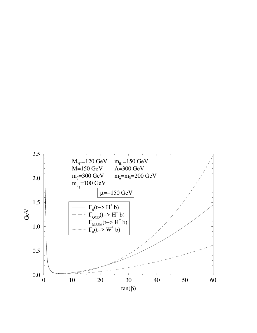
Figure 4.5: The total partial width, $\Gamma_{MSSM}(t\rightarrow H^{+}\,b)$, including all MSSM  effects, versus $\tan\beta$, as compared to the tree-level width and the QCD-corrected width. Also plotted is the tree-level partial width of the standard top quark decay, $t\rightarrow W^{+}\,b$. The masses of the top and bottom quarks are $m_{t}=175\mbox{ GeV}$ and $m_{b}=5\mbox{ GeV}$, respectively, and the rest of the inputs are explicitly given. We remark that $A_{t}=A_{b}=...\equiv A$ is a common value of the trilinear coupling for all squark and slepton generations. Unless explicitly stated otherwise, the inputs staying at fixed values in the remaining figures are common to the values stated here.

Needless to say, a crucial parameter to be investigated is $\tan\beta$. In Fig. 4.5 we plot the tree-level width, $\Gamma_{0}(t\rightarrow H^{+}\,b)$, and the total partial width, $\Gamma_{MSSM}(t\rightarrow H^{+}\,b)$, comprising all the MSSM  effects, as a function of $\tan\beta$. A typical set of parameters is chosen well within canonical expectations (see below); the individual influence of each one of them is tested in Figs. 4.7 to 4.17. Also shown in Fig. 4.5 is the (tree-level) partial width of the standard top quark decay $t\rightarrow W^{+}\,b$, which is (as noted above) far less sensitive to quantum corrections. For convenience, we have included in Fig. 4.5 a plot of $\Gamma_{\rm QCD}(t\rightarrow H^{+}\,b)$, i.e.  the partial width that would be obtained in the presence of only the standard QCD  corrections. Recently it has been shown that EW  corrections in the absence of SUSY particles, i.e.  2HDM effects, can also be large, though it happens for a Higgs spectrum very different of the MSSM  one [61, 62]. On the other hand by simple inspection of Fig. 4.6 we see that the Higgs sector corrections are indeed small, so the QCD  corrected curve is in fact the partial width that would be obtained in a non-SUSY  2HDM under the conditions of the present study.

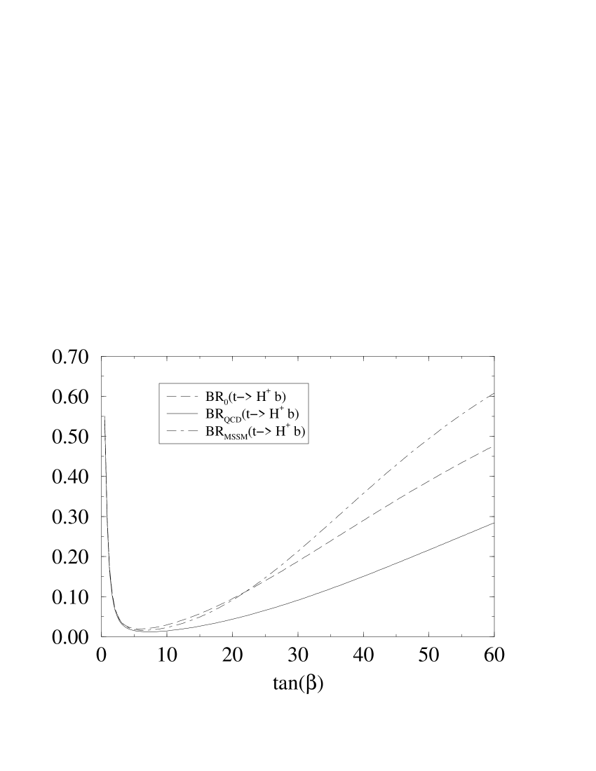
(a)	(b)

Figure 4.6: (a) The relative corrections $\delta$, eq.(4.32), as a function of $\tan\beta$. Shown are the SUSY-EW, standard EW (i.e. non-supersymmetric electroweak), SUSY-QCD, standard QCD, and total MSSM contribution, eq.(4.37); (b) The branching ratio (4.34), as a function of $\tan\beta$; separately shown are the values of this observable after including standard QCD  corrections, full MSSM  corrections, and the tree-level value.

From eq.(4.24) it is clear that, for large (resp.  small) $\tan\beta$, the renormalized form factor yielding the bulk of the SUSY  contribution is $\Lambda_{L}$ (resp. $\Lambda_{R}$). To appraise the relative importance of the various types of MSSM  effects on $\Gamma(t\rightarrow H^{+}\,b)$, in Figs. 4.6(a)-4.6(b) we provide plots for the correction to the partial width, eq.(4.32), and to the branching ratio, eq.(4.34), as a function of $\tan\beta$, reflecting the various individual contributions. Specifically, we show in Fig. 4.6(a):

• (i) The supersymmetric electroweak contribution from genuine ($R$-odd) sparticles (denoted $\delta_{\rm SUSY-EW}$), i.e. from sfermions (squarks and sleptons), charginos and neutralinos;

• (ii) The electroweak contribution from non-supersymmetric ($R$-even) particles ($\delta_{EW}$). It is composed of two distinct types of effects, namely, those from Higgs and Goldstone bosons (collectively called “Higgs” contribution, and denoted $\delta_{\rm Higgs}$) plus the leading SM effects [28, 29, 95] from conventional fermions ($\delta_{\rm SM}$):

  $$\delta_{EW}=\delta_{\rm Higgs}+\delta_{\rm SM}\,;$$ (4.36)

  The remaining non-supersymmetric electroweak effects are subleading and are neglected.

• (iii) The strong supersymmetric contribution (denoted by $\delta_{\rm SUSY-QCD}$) from squarks and gluinos;

• (iv) The strong contribution from conventional quarks and gluons (labeled $\delta_{\rm QCD}$); and

• (v) The total MSSM  contribution, $\delta_{\rm MSSM}$, namely, the net sum of all the previous contributions:

  $$\delta_{\rm MSSM}=\delta_{\rm SUSY-EW}+\delta_{EW}+\delta_{\rm SUSY-QCD}+\delta_{\rm QCD}.$$ (4.37)

In Fig. 4.6(b) we reflect the impact of the MSSM  on the branching ratio, as a function of $\tan\beta$; also shown are the tree-level value of the branching ratio and the latter quantity after including the (non-supersymmetric) QCD corrections. A typical common set of inputs has been chosen in Figs. 4.6(a)-4.6(b) such that the supersymmetric electroweak corrections reinforce the strong supersymmetric effects (SUSY-QCD). For this set of inputs, the total MSSM correction to the partial width of $t\rightarrow H^{+}\,b$ is positive for $\tan\beta>20$ (approx.). Remarkably enough, this is so in spite of the huge negative effects induced by QCD. In fact, we see that the gluon effects are overridden by the gluino effects provided $\tan\beta$ is sufficiently large, to be concrete for $\tan\beta\geq 30$. Beyond this value, the strength of the supersymmetric loops becomes rapidly overwhelming; e.g.  at the representative value $\tan\beta=m_{t}/m_{b}=35$ we find $\delta_{\rm MSSM}\simeq+27\%$; and at $\tan\beta\simeq 50$, which is the preferred value claimed by $SO(10)$ Yukawa coupling unification models [146, 147, 148], the correction is already $\delta_{\rm MSSM}\simeq+55\%$. Quite in contrast, at that $\tan\beta$  one would expect, in the absence of SUSY  effects, a (QCD) correction of about $-57\%$, i.e.  virtually of the same size but opposite in sign!

Coming back to Fig. 4.5, we see that, after including the SUSY  effects, the partial width of $t\rightarrow H^{+}\,b$ equals the partial width of the standard decay $t\rightarrow W^{+}\,b$ near the “$SO(10)$” point $\tan\beta=50$. (The meeting point is actually a bit earlier in $\tan\beta$, after taking into account the known [40, 41], negative, SUSY  corrections to $t\rightarrow W^{+}\,b$, but this effect is not shown in the figure since it is relatively small.) Now, for the typical set of parameter values introduced in Fig. 4.5, the top quark decay width into SUSY  particles, eq.(4.35), is rather tiny. Thus it is not surprising that in these conditions the branching ratio of the charged Higgs mode can be remarkably high: $BR(t\rightarrow H^{+}\,b)\simeq 50\%$, i.e.  basically $50\%-50\%$ versus the standard decay mode. In contrast, the branching ratio without SUSY  effects (i.e.  essentially the QCD-corrected branching ratio) is much smaller: at the characteristic $SO(10)$ value, $\tan\beta=50$, it barely reaches $20\%$. Clearly, if the SUSY  quantum effects are there, they could hardly be missed!

As noted before, even though the dominant MSSM  effects are, by far, the QCD  and SUSY-QCD  ones, they have opposite signs. Therefore, there is a crossover point of the two strongly interacting dynamics, where the conventional QCD loops are fully counterbalanced by the SUSY-QCD  loops. This leads to a funny situation, namely, that at the vicinity of that point the total MSSM  correction is given by just the subleading, albeit non-negligible, electroweak supersymmetric contribution: $\delta_{\rm MSSM}\simeq\delta_{\rm SUSY-EW}$. The crossover point occurs at $\tan\beta\mbox{ \raisebox{-4.0pt}{${\stackrel{{\scriptstyle\textstyle>}}{{\sim}}}$} }32\simeq m_{t}/m_{b}$, where $\delta_{\rm SUSY-EW}\mbox{ \raisebox{-4.0pt}{${\stackrel{{\scriptstyle\textstyle>}}{{\sim}}}$} }20$. For larger and larger $\tan\beta$  beyond $m_{t}/m_{b}$, the total (and positive) MSSM  correction grows very fast, as we have said, since the SUSY-QCD  loops largely over-compensate the standard QCD  corrections. As a result, the net effect on the partial width appears to be opposite in sign to what might naively be “expected” (i.e.  the QCD  sign). Of course, this is not a general result since it depends on the actual values of the MSSM  parameters. In the following we wish to explore the various parameter dependences and in particular we want to assess whether a favourable situation as the one just described is likely to happen in an ample portion of the MSSM  parameter space. In particular, the value $\tan\beta=m_{t}/m_{b}=35$ will be chosen in all our plots where that parameter must be fixed. We consider it as representative of the low end of the high $\tan\beta$  segment, eq.(4.8). Thus $\tan\beta=m_{t}/m_{b}=35$ behaves as a sort of threshold point beyond which the MSSM  quantum effects on $t\rightarrow H^{+}\,b$ take off so fast that they should have indelible experimental consequences on top quark physics.

As regards to the non-supersymmetric electroweak corrections, $\delta_{\rm EW}$, it is apparent from Fig. 4.6(a) that they are very small, especially in the high $\tan\beta$  segment. Also in the very low $\tan\beta$ segment, $0.5\mbox{ \raisebox{-4.0pt}{${\stackrel{{\scriptstyle\textstyle<}}{{\sim}}}$} }\tan\beta\mbox{ \raisebox{-4.0pt}{${\stackrel{{\scriptstyle\textstyle<}}{{\sim}}}$} }1$, $\delta_{EW}$ is relatively small; and this is so not only because both $\delta_{\rm Higgs}$ and $\delta_{\rm SM}$ become never too large in absolute value, but also because in that region there is a cancellation between $\delta_{\rm Higgs}<0$ and $\delta_{\rm SM}>0$. As it happens, we end up with the fact that the complicated Higgs effects result in a very tiny contribution, except in the very low $\tan\beta$  end, where e.g.  they can reach $-15\%$ at $\tan\beta\simeq 0.5$. In this corner of the parameter space, $\delta_{\rm Higgs}$ becomes the dominant part of $\delta_{\rm MSSM}$, being even larger than the QCD  effects, which stay at the level of $-8\%$, and also larger than the SUSY-QCD  and SUSY-EW  corrections, which remain below $+4\%$ and $-1\%$, respectively.

We have treated in detail the very low $\tan\beta$  segment by including the one-loop renormalization of the Higgs masses [112, 113, 114, 115, 116]. This is necessary in order to avoid that the lightest CP-even Higgs mass either vanishes at $\tan\beta=1$ or becomes lighter than the phenomenological bounds near that value. In passing, we have checked that the one-loop shift of the masses, as well as of the CP-even mixing angle, $\alpha$, has little impact on the partial width of $t\rightarrow H^{+}\,b$ in the entire range of $\tan\beta$, eq.(4.6). They entail at most an additional $5\%$ negative shift of $\delta_{\rm MSSM}$ in the very low $\tan\beta$  region. It is precisely in this region where the Higgs effects could be expected of some relevance, and thus where the renormalization of the CP-even mixing angle could have introduced some noticeable change in the neutral Higgs couplings. Quite on the contrary, at high $\tan\beta$  the corresponding effect is found to be of order one per mil and is thus negligibly small. On the other hand, a simple inspection of Figs. 4.5 and 4.6(b) shows that even in the very low $\tan\beta$  ballpark, where there may be some ten percent effect from the Higgs sector, the rising of the tree-level width is so fast that it becomes very hard to isolate these corrections. We conclude that, despite the rather large number of diagrams involved, the over-all yield from the Higgs sector of the MSSM  on $t\rightarrow H^{+}\,b$ is rather meagre in the whole $\tan\beta$  range (4.6). This fact is somewhat surprising and was not obvious a priori, due to the presence of enhanced Yukawa couplings (1.2) in the whole plethora of Higgs diagrams. The cancellations involved are reminiscent of the scanty SUSY  Higgs effects obtained for the standard top quark decay $t\rightarrow W^{+}\,b$ [161, 162].

We come now to briefly discuss the standard QCD  effects up to ${\cal O}(\alpha_{s})$, which involve one-loop gluon corrections and gluon bremsstrahlung [43, 44]. As it is plain from Fig. 4.6(a), $\delta_{\rm QCD}$ is negative-definite and very important in the high $\tan\beta$ segment. It quickly saturates for $\tan\beta\mbox{ \raisebox{-4.0pt}{${\stackrel{{\scriptstyle\textstyle>}}{{\sim}}}$} }10$ at a large value of order $-60\%$. Therefore, the QCD  effects need to be considered in order to isolate the virtual SUSY  signature [44, 43]. The leading behaviour of the standard QCD  component in the relative correction (4.32) can be easily assessed by considering the following asymptotic formula

$$\delta_{QCD}=-\frac{2\,\alpha_{s}}{3\pi}\;\frac{\frac{8\pi^{2}-15}{12}(m^{2}_{b}\tan^{2}\beta+m^{2}_{t}\cot^{2}\beta)+3(4+\tan^{2}\beta-2\frac{M^{2}_{H^{+}}}{m^{2}_{t}}\cot^{2}\beta)m^{2}_{b}\ln\left(\frac{m^{2}_{t}}{m^{2}_{b}}\right)}{m^{2}_{b}\tan^{2}\beta+m^{2}_{t}\cot^{2}\beta}\,,$$ (4.38)

which is obtained by expanding the exact one-loop formula up to ${\cal O}(m_{b}^{2}/m_{t}^{2},M_{H^{+}}^{2}/m_{t}^{2})$. Here $\alpha_{s}\equiv\alpha_{s}(m_{t}^{2})$, normalized as $\alpha_{s}(M_{Z}^{2})\simeq 0.12$. The big log factor $\ln(m^{2}_{t}/m^{2}_{b})$ originates from the running b-quark mass evaluated at the top quark scale. The correction is seen to be always negative. We point out that while we have used the exact ${\cal O}(\alpha_{s})$ formula for the numerical evaluation, the approximate expression given above is sufficiently accurate to convey the general features to be expected both at low and at high $\tan\beta$. In particular, for $m_{b}\neq 0$ and $\tan\beta$  in the relevant high segment (4.8), the QCD  correction becomes very large and saturates at the value

$$\delta_{QCD}=-\frac{2\,\alpha_{s}}{\pi}\;\left(\frac{8\pi^{2}-15}{36}+\ln\frac{m^{2}_{t}}{m^{2}_{b}}\right)\simeq-62\%\,\ \ \ (\tan\beta>>\sqrt{m_{t}/m_{b}}\simeq 6)\,.$$ (4.39)

(The exact ${\cal O}(\alpha_{s})$ formula gives slightly below $-60\%$.) At low values of $\tan\beta$, the corrections are much smaller, as it follows from the approximate expression $\delta_{\rm QCD}\simeq(-\alpha_{s}/\pi)(8\pi^{2}-15)/18\simeq-12\%$. We remark that for $m_{b}=0$ the dependence on $\tan\beta$ totally disappears from eq.(4.38), so that one would never be able to suspect the large contribution (4.39) in the high $\tan\beta$  regime. The limit $m_{b}=0$, nevertheless, has been considered for the standard QCD  corrections in some places of the literature but, as we have seen, it is untenable unless one concentrates on values of $\tan\beta$  of order $1$, in which case the relevance of our decay for SUSY  is doomed to oblivion. This situation is similar to the one mentioned above concerning the SUSY-QCD  corrections in the limit $m_{b}=0$, which leads to an scenario totally blind to the outstanding supersymmetric quantum effects obtained for $m_{b}\neq 0$ at high $\tan\beta$ [42, 48]. We stress that in spite of the respectable size of the standard QCD  effects, they become fast stuck at the saturation value (4.39), which is independent of $\tan\beta$. On the contrary, the SUSY-QCD  effects grow endlessly with $\tan\beta$  and thus rapidly overtake the standard QCD  prediction.

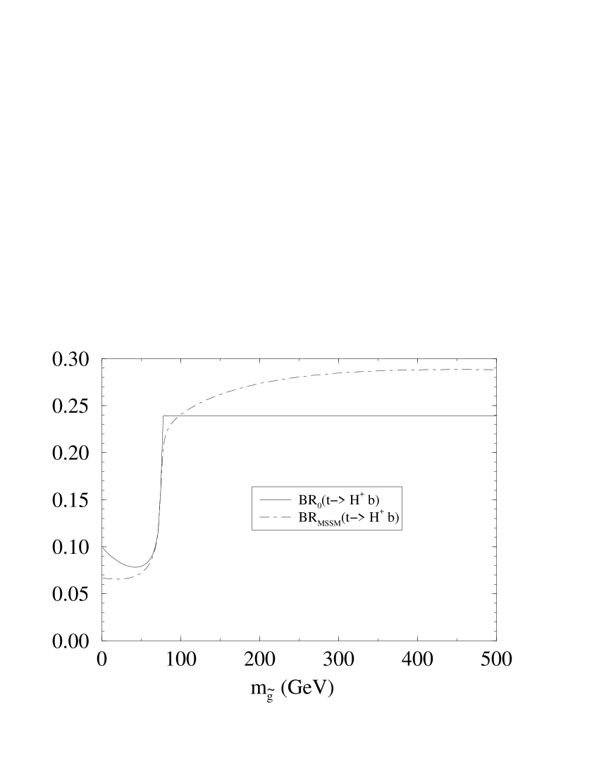
(a)	(b)

Figure 4.7: (a) The relative corrections $\delta$, eq.(4.32), as a function of the gluino mass, $m_{\tilde{g}}$, for the SUSY-EW, standard EW, SUSY-QCD, standard QCD  contributions, and total MSSM  contribution, (b) As in (a), but for the tree-level and full MSSM-corrected branching ratios (4.34). We have set $\tan\beta=m_{t}/m_{b}=35$. This value is maintained in all figures where $\tan\beta$ is fixed.

Worth noticing is the evolution of the quantities (4.32) and (4.34) as a function of the gluino mass (Cf. Figs. 4.7(a)-4.7(b)). Of course, only the SUSY-QCD  component is sensitive to $m_{\tilde{g}}$. Although the SUSY-QCD  effects have been object of a particular study in Ref.[42, 48], we find it convenient, to ease comparison, to display the corresponding results in the very same conditions in which the electroweak supersymmetric corrections are presented. The steep falls in Fig. 4.7(a) are associated to the presence of threshold effects occurring at points satisfying $m_{\tilde{g}}+m_{\tilde{t}_{1}}\simeq m_{t}$. An analogous situation was observed in Ref.[40, 41, 42] for the SUSY corrections to the standard top-quark decay. Away from the threshold points, the behaviour of $\delta_{SUSY-QCD}$ is smooth and perfectly consistent with perturbation theory. In Fig. 4.7(b), where the branching ratio (4.34) is plotted, the steep falls at the threshold points are no longer present since they are compensated for by the simultaneous opening of the two-body supersymmetric mode $t\rightarrow\tilde{t}_{1}\,\tilde{g}$, for $m_{\tilde{g}}<m_{t}-m_{\tilde{t}_{1}}$.

We emphasize that the relevant gluino mass region for the decay $t\rightarrow H^{+}\,b$ is not the light gluino region, but the heavy one, the reason being that the important self-energy correction mentioned above, eq.(4.29), involves a gluino mass insertion. As a consequence, virtually for any set of MSSM  parameters, there is a well sustained SUSY  correction for any gluino mass above a certain value, in our case $m_{\tilde{g}}\mbox{ \raisebox{-4.0pt}{${\stackrel{{\scriptstyle\textstyle>}}{{\sim}}}$} }250-300\mbox{ GeV}$. The correction raises with the gluino mass up to a long flat maximum before bending –very gently – into the decoupling regime (far beyond $1\mbox{ TeV}$) [42, 48]. The fact that the decoupling rate of the gluinos appears to be so slow has an obvious phenomenological interest.

Next we consider in detail the sensitivity of our decay on the higgsino-gaugino parameters $(\mu,M)$ characterizing the chargino-neutralino mass matrices (Cf. section 2.3). We start with the supersymmetric Higgs mixing mass, $\mu$. As already stated above, we will largely concentrate on the $\mu<0$ case. Together with $A_{t}>0$ this yields $A_{t}\,\mu<0$, which is a sufficient condition [148, 164, 165, 166, 167, 168, 169, 170] (see also section 4.5) for the MSSM  prediction on $BR(b\rightarrow s\,\gamma)$ to be compatible with experiment in the presence of a relatively light charged Higgs boson (as the one participating in the top decay under study). In fact, it is known that charged Higgs bosons of ${\cal O}(100)\mbox{ GeV}$ interfere constructively with the SM amplitude and would render a final value of $BR(b\rightarrow s\,\gamma)$ exceedingly high. Fortunately, this situation can be remedied in the MSSM  since the alternative contribution from charginos and stops tends to cancel the Higgs contribution provided that $A_{t}\,\mu<0$. Furthermore, one must also require relatively light values for the masses of the lightest representatives of these sparticles, as well as high values of $\tan\beta$ [148, 164, 165, 166, 167, 168, 169, 170]; hence one is led to a set of conditions which fit in with nicely to build up a favourable scenario for the decay $t\rightarrow H^{+}\,b$.

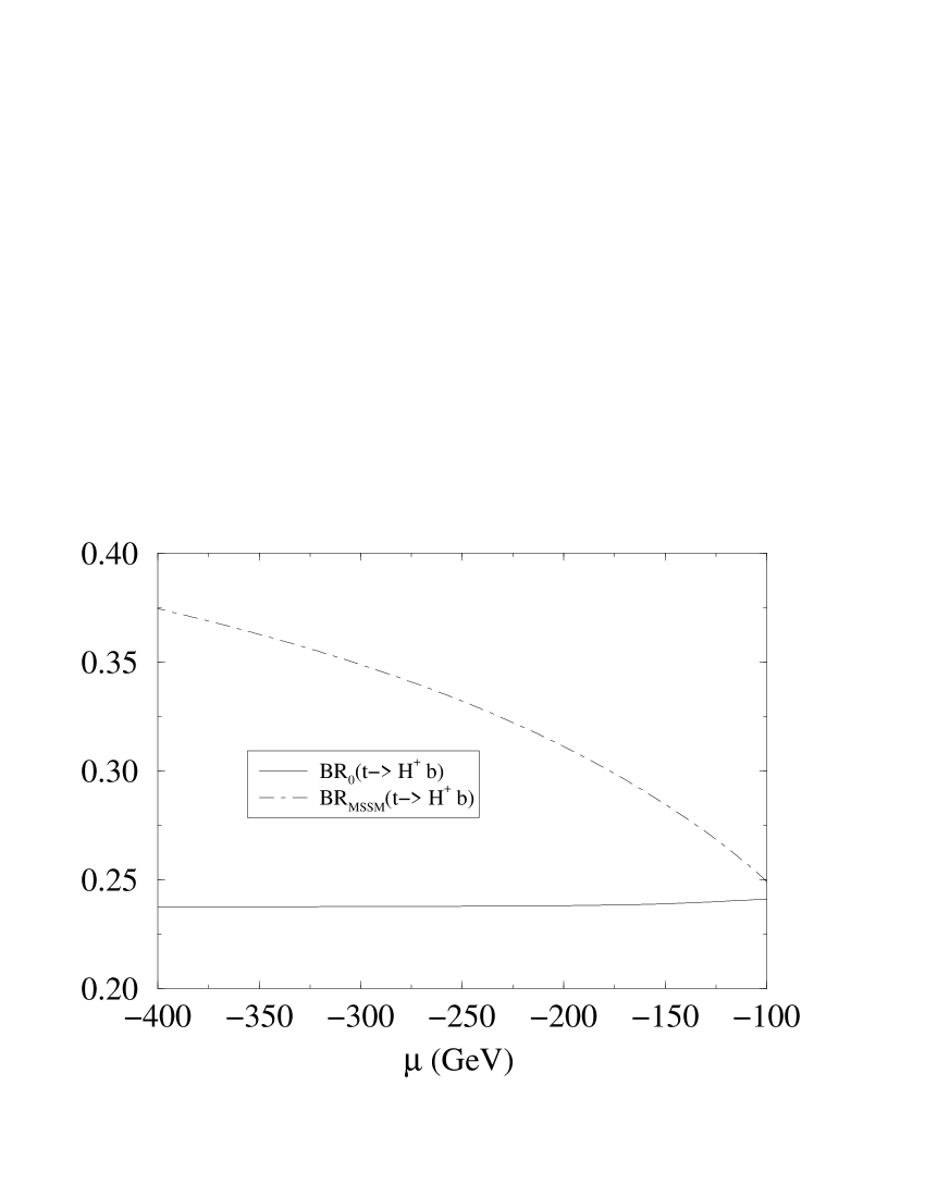
(a)	(b)

Figure 4.8: (a) The relative corrections $\delta$, eq.(4.32), as a function of the supersymmetric Higgs mixing parameter, $\mu$, for the various contributions as in Fig.4.6(a); (b) As in (a), but for the same branching ratios as in Fig. 4.7(b).

The evolution of the individual contributions (4.37), together with the total MSSM  yield, as a function of $\mu<0$, is shown in Figs. 4.8(a)-4.8(b) for given values of the other parameters. We immediately gather from these figures that the SUSY-QCD  correction is extremely sensitive to $\mu$. In fact, $\delta_{\rm SUSY-QCD}$ grows rather fast with $|\mu|$. This is already patent at the level of the leading $\delta m_{b}/m_{b}$ effect given by eq.(4.29). In all figures where a definite $\mu<0$ is to be chosen, we have taken the moderate value $\mu=-150\mbox{ GeV}$.

Concerning the electroweak contribution, we noted above that the component $\delta m_{b}/m_{b}$, eq.(4.31), actually decreases with $\mu$. However, the $\mu$ dependences in the full $\delta_{\rm SUSY-EW}$ are more complicated than in $\delta_{\rm SUSY-QCD}$ and cannot be read off eq.(4.31). This is evident from Fig. 4.8(a) where the total $\delta_{\rm SUSY-EW}$ is fairly insensitive to $\mu$; $\delta_{\rm MSSM}$, therefore, inherits its marked $\mu$-dependence basically from the SUSY-QCD  component. As for the sensitivity of the corrections on the $SU(2)_{L}$-gaugino soft SUSY-breaking parameter, $M$, Fig. 4.9 conveys immediately that it is virtually non-existent.

Figure 4.9: Dependence of $\delta$, eq.(4.32), on the $SU(2)_{L}$-gaugino soft SUSY-breaking mass, $M$, assuming that the $U(1)_{Y}$ gaugino mass, $M^{\prime}$, is related to $M$ through $M^{\prime}/M={5\over 3}\,\tan^{2}\theta_{W}$. The same individual and total contributions as in Fig.4.6(a) are shown.

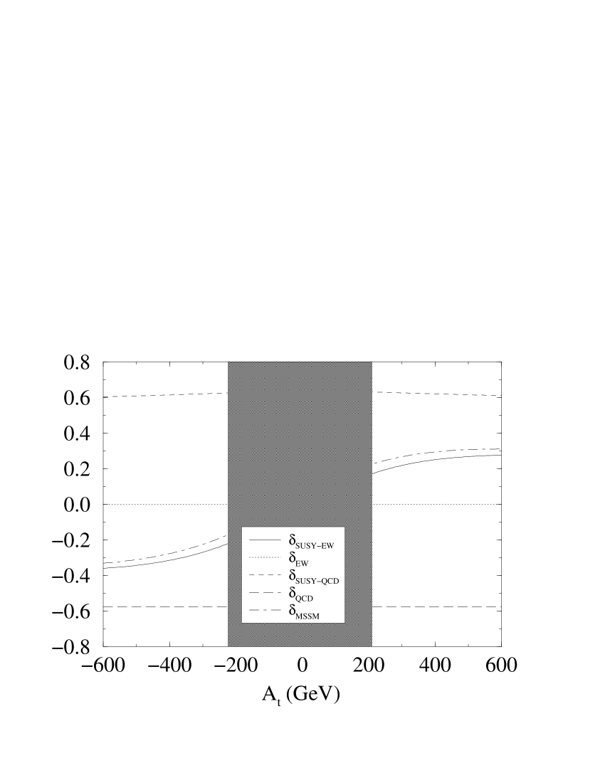
(a)	(b)

Figure 4.10: (a) The relative corrections $\delta$, eq.(4.32), as a function of the trilinear soft SUSY-breaking parameter $A_{b}$ in the bottom sector. The other trilinear couplings are kept as in Fig.8; (b) As in (a), but for the trilinear soft SUSY-breaking parameter $A_{t}$ in the top sector. Shown are the same individual and total contributions as in Fig.4.6(a).

There is some slight evolution of the corrections with $A_{b}$ (Fig. 4.10(a)), mainly on the SUSY-QCD  side. We realize that $\delta_{\rm SUSY-QCD}$ is not perfectly symmetric with respect to the sign of $A_{b}$. Once the sign $\mu<0$ is chosen, the correction is larger for negative values of $A_{b}$ than for positive values. We have erred on the conservative side by choosing $A_{b}=+300\mbox{ GeV}$ wherever this parameter is fixed. As far as $A_{t}$ is concerned, $\delta_{\rm SUSY-QCD}$ can only evolve as a function of that parameter through vertex corrections, which are proportional to $A_{t}\,\cot\beta$ (Cf. section 2.4.3); however, at large $\tan\beta$  these are very depressed. The electroweak correction $\delta_{\rm SUSY-EW}$, instead, is very much dependent on $A_{t}$; indeed, a typical component exhibiting this behaviour is given by eq.(4.31), which is linear in $A_{t}$. The full dependence, however, is not linear and is recorded in Fig. 4.10(b). We realize that $\delta_{\rm SUSY-EW}$ and $\delta_{\rm MSSM}$ change sign with $A_{t}$. The shaded vertical band in Fig. 4.10(b) is excluded by our choice of parameters in Fig. 4.5.

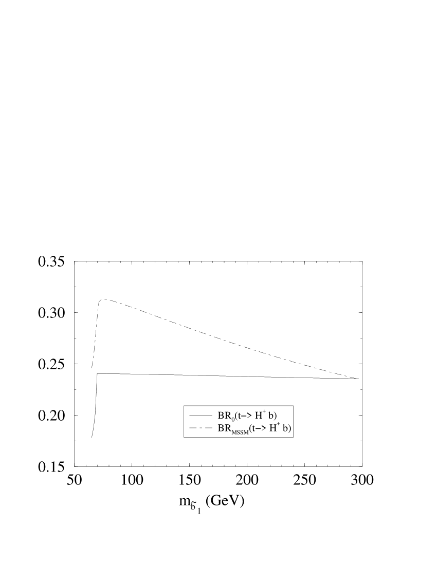
(a)	(b)

Figure 4.11: (a) The relative corrections $\delta$, eq.(4.32), as a function of the lightest sbottom mass, $m_{\tilde{b}_{1}}$, for the various contributions as in Fig.4.6(a); (b) As in (a), but for the same branching ratios as in Fig.4.7(b).

Another very crucial parameter to be investigated is the value of $m_{\tilde{b}_{1}}$. This is because the SUSY-QCD  correction hinges a great deal on the value of the sbottom masses, as it is plain from eq.(4.29). As a matter of fact, a too large a value of $m_{\tilde{b}_{1}}$ may upside down the leadership of the SUSY-QCD  effects. As a typical mass value for all squarks other than the stop we use $m_{\tilde{q}}\geq 150-200\mbox{ GeV}(\tilde{q}\neq\tilde{t})$. From Fig. 4.11(a) we see that provided $m_{\tilde{b}_{1}}\mbox{ \raisebox{-4.0pt}{${\stackrel{{\scriptstyle\textstyle<}}{{\sim}}}$} }300\mbox{ GeV}$ the SUSY-QCD  effects remain dominant, but they steadily go down the larger is $m_{\tilde{b}_{1}}$. The electroweak correction $\delta_{SUSY-EW}$, on the other hand, is quite sustained with increasing $m_{\tilde{b}_{1}}$ and there are parameter configurations where for sufficiently heavy sbottoms the supersymmetric electroweak effects are larger than the SUSY-QCD  effects. However, this is not the most likely situation. The behaviour of the branching ratio is plotted in Fig. 4.11(b).

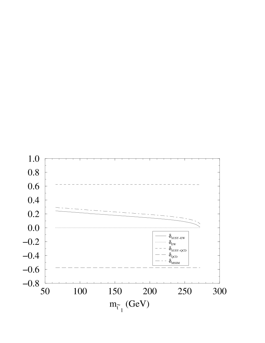
Figure 4.12: The relative corrections $\delta$, eq.(4.32), as a function of the lightest stop mass, $m_{\tilde{t}_{1}}$, for the various contributions as in Fig.4.6(a).

Obviously, the evolution of the SUSY-QCD corrections with the stop masses is basically flat (Fig. 4.12) since the leading contribution is independent of $m_{\tilde{t}_{1}}$. Therefore, for definiteness we fix $m_{\tilde{t}_{1}}\simeq 100\mbox{ GeV}$. Nonetheless, if we wish to keep $\delta_{\rm MSSM}>0$, we cannot go too far with $m_{\tilde{t}_{1}}$, for the electroweak correction is also seen to decrease with $m_{\tilde{t}_{1}}$. Indeed, whereas for $m_{\tilde{t}_{1}}=65-100\mbox{ GeV}$ one has $\delta_{\rm SUSY-EW}\mbox{ \raisebox{-4.0pt}{${\stackrel{{\scriptstyle\textstyle>}}{{\sim}}}$} }20\%$, for $m_{\tilde{t}_{1}}\mbox{ \raisebox{-4.0pt}{${\stackrel{{\scriptstyle\textstyle>}}{{\sim}}}$} }250\mbox{ GeV}$ one finds $\delta_{\rm SUSY-EW}\mbox{ \raisebox{-4.0pt}{${\stackrel{{\scriptstyle\textstyle<}}{{\sim}}}$} }10\%$. For heavier stop masses, $\delta_{\rm MSSM}$ becomes zero or slightly negative. In this situation, the imprint of SUSY lies in the fact that the total quantum effect is not as negative as predicted by standard QCD, eq.(4.39).

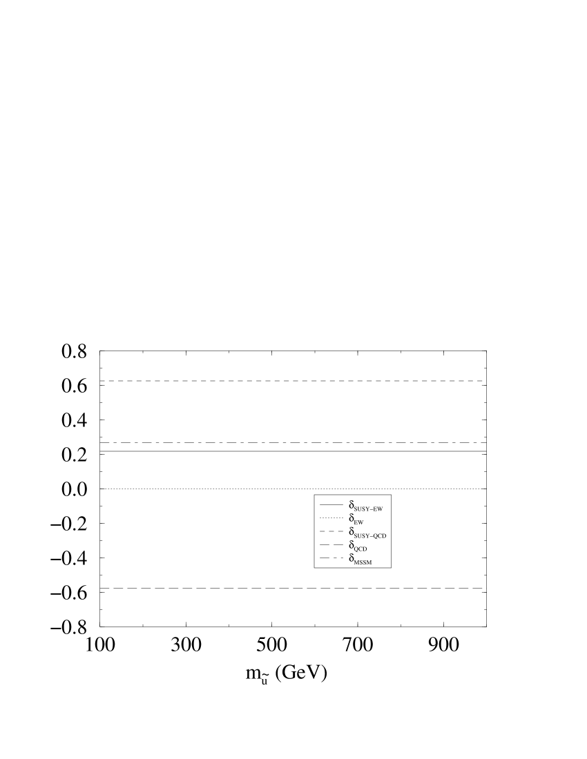
(a)	(b)

Figure 4.13: (a) The relative corrections $\delta$, eq.(4.32), as a function of the up-squark masses $m_{\tilde{u}}\equiv m_{\tilde{u}_{1}}=m_{\tilde{u}_{2}}$. The c-squarks are assumed to be degenerate with the up-squarks; (b) $\delta$ as a function of the sneutrino masses, assumed to be degenerate.

The influence from the sleptons and the other squarks is practically irrelevant as it is borne out by Figs. 4.13(a)-4.13(b). They enter the correction through oblique (universal) quantum corrections. The only exception are the $\tau$-sleptons $\tilde{\tau}_{a}$ (“staus”), since they are involved in the process-dependent (non-oblique) contribution eq.(3.53), where the $\tau$-lepton Yukawa coupling becomes enhanced at large $\tan\beta$. For this reason, $\delta_{\rm SUSY-EW}$ in Fig. 4.13(b) is somewhat larger the smaller is the $\tau$-sneutrino mass (assumed to be degenerate with the other sneutrinos). In all our calculation we have fixed the common sneutrino mass at $200\mbox{ GeV}$.

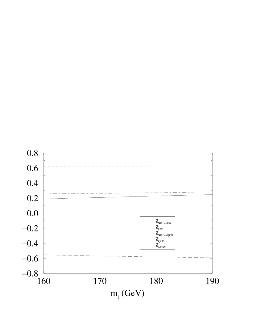
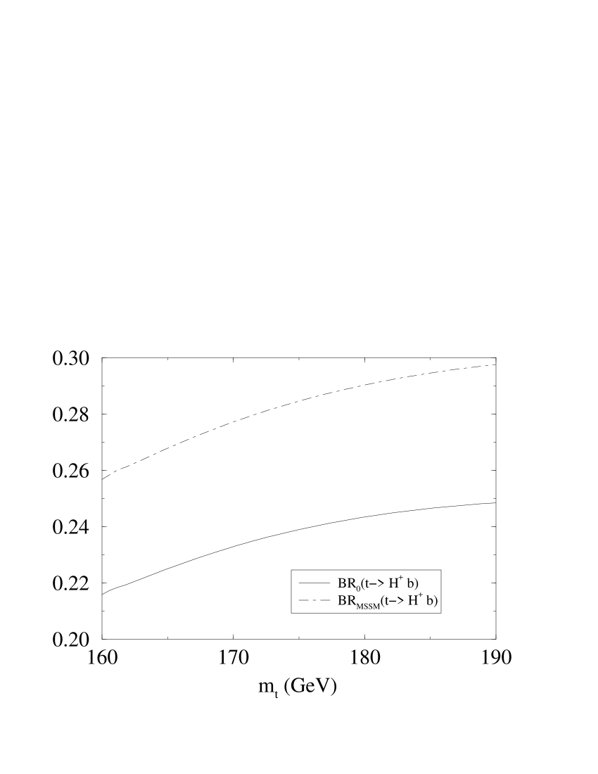
(a)	(b)

Figure 4.14: (a) The relative corrections $\delta$, eq.(4.32), as a function of the top quark mass within about $2\,\sigma$ of the present experimental range at the Tevatron. (b) As in (a), but for the same branching ratios as in Fig.4.7(b).

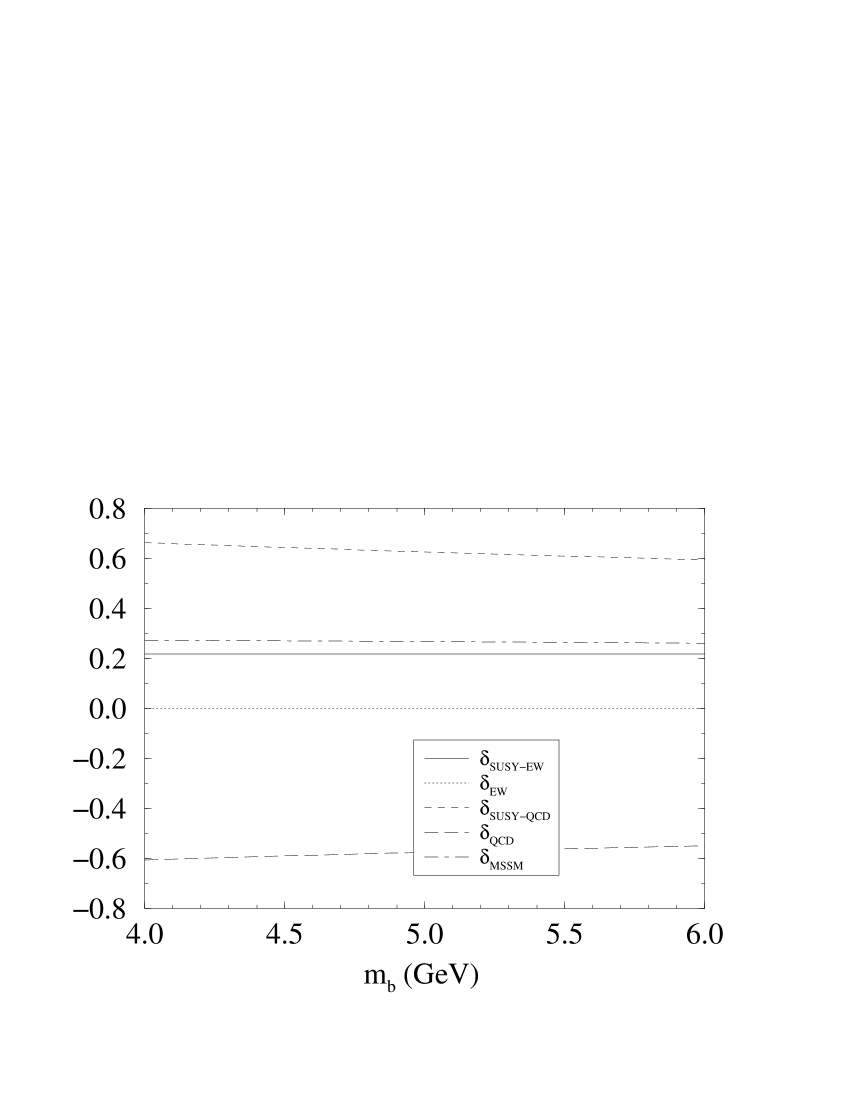
(a)	(b)

Figure 4.15: (a) The relative correction $\delta$, eq.(4.32), as a function of the bottom quark mass. (b) As in (a), but for the same branching ratios as in Fig.4.7(b).

We have also tested the variation of our results as a function of the external particle masses, namely the masses of the top quark, bottom quark and charged Higgs. As for the external fermion masses, the corrections themselves are not very sensitive (see Figs. 4.14(a) and 4.15(a)). Among the SUSY  corrections, the most sensitive one on $m_{t}$ (respectively on $m_{b}$) is $\delta_{\rm SUSY-EW}$ (resp. $\delta_{\rm SUSY-QCD}$). The branching ratios also show some dependence (Figs. 4.14(b) and 4.15(b)), especially on $m_{b}$. This effect is mainly due to the variation of the tree-level partial widths as a function of $m_{t}$ and $m_{b}$. As for the charged Higgs mass, $M_{H^{+}}$, up to now it has been fixed at $M_{H^{+}}=120\mbox{ GeV}$, which is the preferred value for this mass at large $\tan\beta$ [82]. We confirm from Fig. 4.16(a) that there is nothing special in the chosen value for that parameter since the sensitivity of the correction is generally low, except near the uninteresting boundary of the phase space where the branching ratio (Fig. 4.16(b)) boils down to zero.

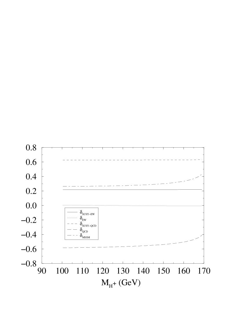
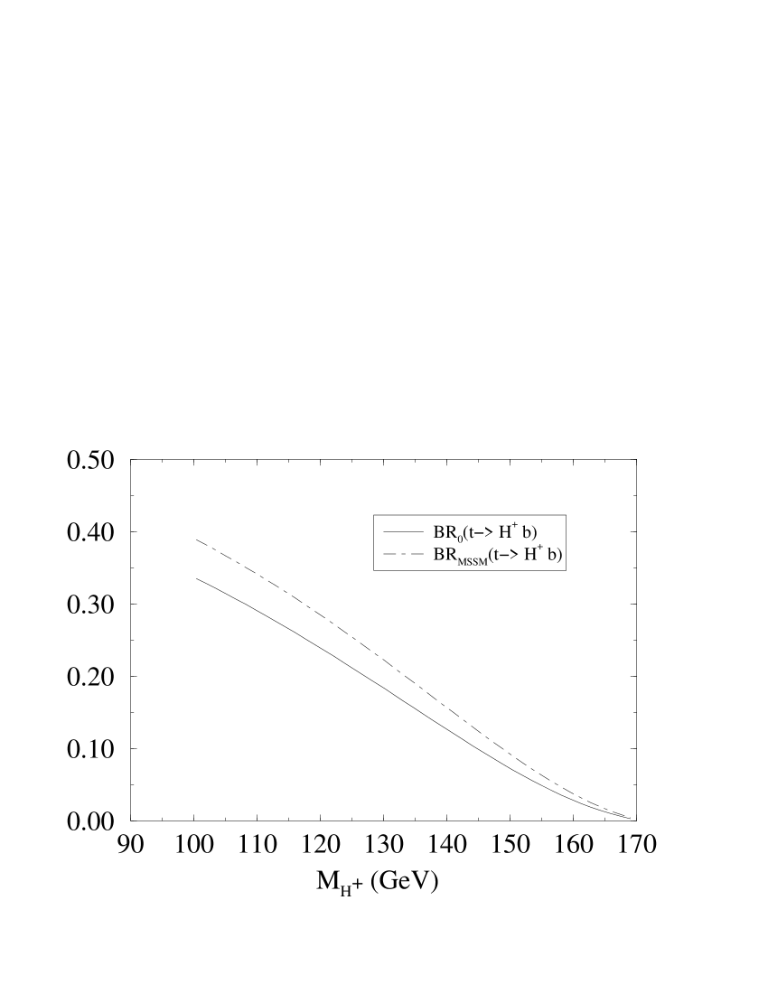
(a)	(b)

Figure 4.16: (a) The relative corrections $\delta$, eq.(4.32), as a function of the charged Higgs mass; (b) As in (a), but for the same branching ratios as in Fig.4.7(b).

Figure 4.17: The supersymmetric ($\delta\tau_{\rm SUSY-EW}$) and non-supersymmetric ($\delta\tau_{\rm EW}$) electroweak contributions to $\delta$, eq.(4.32), from the process-dependent term $\Delta_{\tau}$, eq.(3.53), as a function of $\tan\beta$.

We close our study of the corrections in the $\mu<0$ case by plotting $\delta_{\tau}$ as a function of $\tan\beta$ (see Fig. 4.17). By definition, $\delta_{\tau}$ is that part of $\delta_{\rm MSSM}$ originating from the full process-dependent term $\Delta_{\tau}$, eq.(3.53), which stems from our definition of $\tan\beta$  on eq.(3.50). This piece of information is relevant enough. In fact, it should be recalled that the quantum corrections described in the previous figures are scheme dependent. In particular, they rely on our definition of $\tan\beta$  given on eq.(3.50). What is not scheme dependent, of course, is the predicted value of the width and branching ratio (Figs. 4.5 and 4.6(b)) after including all the radiative corrections. Now, from Fig. 4.17 it is clear that the $\Delta_{\tau}$-term is not negligible, and so there is a process-dependence in our definition of $\tan\beta$, as it was announced in chapter 3. At first sight, the $\delta_{\tau}$-effects are not dramatic since they are small as compared to $\delta_{\rm SUSY-QCD}$, but since the latter is canceled out by standard QCD  we end up with $\delta_{\tau}$ being of the order (roughly half the size) of the electroweak correction $\delta_{\rm SUSY-EW}$.

The main source of process-dependent $\delta_{\tau}$-effects lies in the corrections generated by the $\tau$-mass counterterm, $\delta m_{\tau}/m_{\tau}$, and can be easily picked out in the electroweak-eigenstate basis (see Fig. 4.18) much in the same way as we did for the $b$-mass counterterm. There are, however, some differences, as can be appraised by comparing the diagrams in Figs. 4.4 and 4.18, where we see that in the latter case the effect derives from diagrams involving $\tau$-sleptons with gauginos or mixed gaugino-higgsinos. An explicit computation of the diagrams (a) $+$ (b) in Fig. 4.18 yields

$${\delta m_{\tau}\over m_{\tau}} = {g^{\prime 2}\over 16\pi^{2}}\,\mu\,M^{\prime}\,\tan\beta\,I(m_{\tilde{\tau}_{1}},m_{\tilde{\tau}_{2}},M^{\prime})$$ (4.40)

$$+ {g^{2}\over 16\pi^{2}}\,\mu\,M\,\tan\beta\,I(\mu,m_{\tilde{\nu}_{\tau}},M)\,,$$

where $g^{\prime}=g\,s_{W}/c_{W}$ and $M^{\prime},M$ (Cf. section 2.4.4) are the Soft-SUSY-Breaking Majorana masses associated to the bino $\tilde{B}$ and winos $\tilde{W}^{\pm}$, respectively, and the function $I(m_{1},m_{2},m_{3})$ is again given by eq.(4.30). In the formula above we have projected, from the bino diagram in Fig. 4.18(a), only the leading piece which is proportional to $\tan\beta$. Even so, the contribution from the wino-higgsino diagram in Fig. 4.18(b) is much larger. Numerical evaluation of the sum of the two contributions on eq.(4.40) indeed shows that it reproduces to within few percent the full numerical result (Cf. Fig. 4.17) previously obtained in the mass-eigenstate basis, thus confirming that eq.(4.40) gives the leading contribution. In practice, for a typical choice of parameters as in Fig. 4.5, this contribution is approximately canceled out by part of the electroweak supersymmetric corrections associated to the original process $t\rightarrow H^{+}\,b$, and one is effectively left with eq.(4.31) as being the main source of electroweak supersymmetric quantum effects at high $\tan\beta$.

(0,10)(0,-20) (180,90) thin i1 o1 fermion,label=$\tau_{L}$,label.side=lefti1,v1 plain,label=$\tilde{B}$,tension=0.5v1,v2 dashes,label=,left,tension=0.5v1,v2 fermion,label=$\tau_{R}$,label.side=leftv2,o1 phantom,label=$\tilde{\tau}_{L}$,label.side=left,label.dist=.4cm,tension=0v1,v3 phantom,label=$\tilde{\tau}_{R}$,label.side=left,label.dist=.4cm,tension=0v3,v2 label=$m_{\tau}\ M_{LR}^{\tau}$,label.angle=90,label.dist=.3cm,decor.shape=crossv3 .5w,.84hv3

(0,10)(0,-20) (180,90) thin i1 o1 fermion,label=$\tau_{L}$,label.side=lefti1,v1 phantom,label=,tension=0.5v1,v2 plain,label=$\tilde{W}$,tension=0v1,v4 plain,label=$\tilde{H}_{2}$,tension=0v4,v5 plain,label=$\tilde{H}_{1}$,tension=0v5,v2 dashes,label=$\tilde{\nu}_{\tau}$,left,tension=0.5v1,v2 fermion,label=$\tau_{R}$,label.side=leftv2,o1 decor.shape=crossv4 decor.shape=crossv5 .43w,.5hv4 .57w,.5hv5

(a)

(b)

Figure 4.18: Leading supersymmetric electroweak contributions to $\delta m_{\tau}/m_{\tau}$ in the electroweak-eigenstate basis.

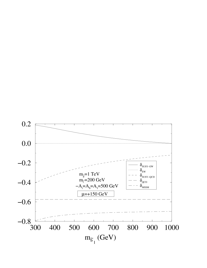
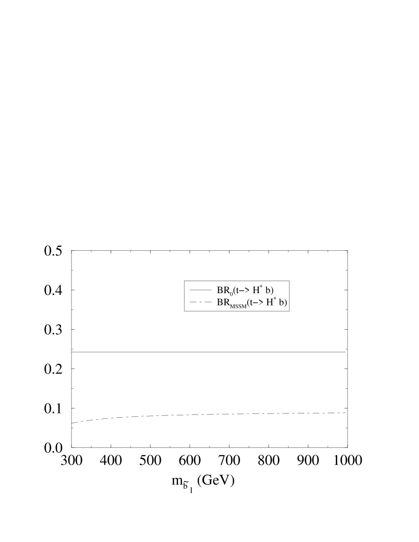
(a)	(b)

Figure 4.19: (a) The relative corrections $\delta$, eq.(4.32), as a function of the lightest sbottom quark mass, for positive $\mu=+150\mbox{ GeV}$, negative $A_{t}$ and given values of the other parameters. In this case, huge values of $m_{\tilde{b}_{1}}$ are needed in order to damp the absolute value of the total correction down to $100\%$; (b) As in (a), but for the same branching ratios as in Fig.4.7(b).

Finally, the corrections corresponding to the case $\mu>0$ are studied in Figs. 4.19(a) and 4.19(b). The problem with $\mu>0$ is that, then, the large SUSY-QCD  corrections have the same (negative) sign as the conventional QCD  effects, and as a consequence the total MSSM  correction can easily blow up above $100\%$, the branching ratio becoming negative! To avoid this disaster (from the point of view of perturbation theory), we enforce the SUSY-QCD  correction to be smaller than in the $\mu<0$ case by assuming an “obese SUSY  scenario” characterized by very large values for the sbottom mass ($m_{\tilde{b}_{1}}=600\mbox{ GeV}$) and the gluino mass ($m_{\tilde{g}}=1000\mbox{ GeV}$). We also choose $A_{t}<0$ so that the electroweak SUSY correction becomes opposite in sign to the SUSY-QCD  correction (a feature that also applies in the $\mu<0$ case, see Fig. 4.10(b)) and in this way the total SUSY  correction is further lessened in absolute value. Incidentally, we remark that the simultaneous sign change of both $\mu$ and $A_{t}$ is also necessary in order to keep $A_{t}\,\mu<0$; as noted above, this is required in order that the MSSM  can be compatible with $BR(b\rightarrow s\,\gamma)$ in the presence of a relatively light charged Higgs. In Fig. 4.20 we bring forward the effect of the new situation on the total partial width. In the present instance, the physical signature would be to measure a partial width significantly smaller than the one predicted by QCD. Clearly, the $\mu>0$ ($A_{t}\,\mu<0$) scenario is not as appealing as the $\mu<0$ ($A_{t}\,\mu<0$) one.

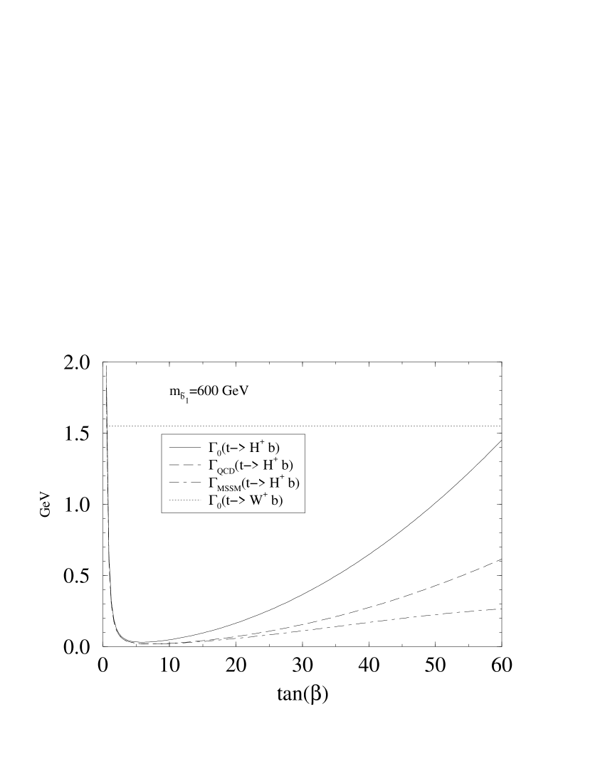
Figure 4.20: The total partial width, $\Gamma(t\rightarrow H^{+}\,b)$, including all MSSM effects, versus $\tan\beta$, for the same inputs as in Fig.4.19(a), as compared to the tree-level width and the QCD-corrected width. A typical value of $m_{\tilde{b}_{1}}$ within the range used in Fig.4.19(a) is selected. Also plotted is the tree-level partial width of the standard top quark decay $t\rightarrow W^{+}\,b$.

4.5 Implications for the Tevatron data

The results presented in previous sections indicate that the SUSY  corrections to the decay under study could have a great impact on the search for charged Higgs bosons at the Tevatron. The CDF Collaboration at the Tevatron has carried out direct searches for charged Higgs production in $p\,\bar{p}$ collisions at $\sqrt{s}=1.8\mbox{ TeV}$ [134, 171, 172]. In these studies one is concerned with the final configurations $t\bar{t}\rightarrow H^{+}\,H^{-}\,b\,\bar{b},W^{+}\,H^{-}\,b\,\bar{b},H^{+}\,W^{-}\,b\,\bar{b}$. The latter would differ from that of the standard model, $t\bar{t}\rightarrow W^{+}\,W^{-}\,b\,\bar{b}$, by an excess of states with one (or two) $\tau$-lepton “jets” (i.e.  usually tagged in the hadronic decay mode) and two b-quarks and large missing transverse energy associated to the decays $H^{+}\rightarrow\tau^{+}\,\nu_{\tau}$ and/or $H^{-}\rightarrow\tau^{-}\,\bar{\nu}_{\tau}$.

As stated in section 4.2, if $M_{H^{\pm}}$ is not too close to the phase space limit, then there are two regimes, namely a low and a high $\tan\beta$ regime, where the partial width of the unconventional top quark decay becomes sizeable as compared to the standard decay $t\rightarrow W^{+}\,b$. Nevertheless we shall focus only on the high $\tan\beta$ regime as it is this case that is correlated with the Higgs maximum rate into the $\tau$-mode versus the hadronic mode (Cf.  eq.(4.7)). Clearly, the identification of the charged Higgs decay of the top quark could be a matter of observing a departure from the universality prediction for all the lepton channels through the measurement of an excess of inclusive (hadronic) $\tau$-events. However, from the non-observation of any $\tau$-lepton surplus, one may determine an exclusion region in the $(\tan\beta,M_{H})$-plane  [134, 171, 172, 173] for any (Type II) $2HDM$ [39]. The region highlighted in this plane consists of a sharply edged area forbidding too high values of $\tan\beta$ in correlation with $M_{H^{\pm}}$. In the relevant SUSY  region $M_{H^{\pm}}>100\mbox{ GeV}$ (see below) the most recent analysis would imply that values in the range $\tan\beta\mbox{ \raisebox{-4.0pt}{${\stackrel{{\scriptstyle\textstyle>}}{{\sim}}}$} }40$ would be excluded [171, 172].

In spite of its foreseeable importance, the impact of the SUSY quantum corrections on the dynamics of $t\rightarrow H^{+}\,b$ was not included in any of the aforementioned analysis [134, 171, 172, 173]. And this is especially significant in a decay like $t\rightarrow H^{+}\,b$ whose sole existence could, in a sense, already be an indirect sign of SUSY. For, as is well-known, the CLEO data [174] on the radiative decays $\bar{B}^{0}\rightarrow X_{s}\,\gamma$ (viz. $b\rightarrow s\,\gamma$) set a rather stringent lower bound on the mass of any charged Higgs scalar belonging to a generic $2HDM$, to wit: $M_{H^{\pm}}>240\mbox{ GeV}$. Therefore, with only the $W^{\pm}$ and $H^{\pm}$ electroweak corrections, the charged Higgs mass is forced to lie in a range where the decay $t\rightarrow H^{+}\,b$ becomes kinematically blocked up. Of course, this is so because the virtual Higgs effects go in the same direction as the SM  contribution. Fortunately, this situation can be remedied in the MSSM where the complete formula for the $b\rightarrow s\,\gamma$ branching ratio reads (see the extensive literature [148, 164, 165, 166, 167, 168, 169, 170] for details):

$$BR(b\rightarrow s\,\gamma)\simeq BR(b\rightarrow c\,e\,\bar{\nu})\,{(6\,\alpha_{\rm em}/\pi)\,\left(\eta^{16/23}\,A_{\gamma}+C\right)^{2}\over I(m_{c}/m_{b})\,\left[1-\frac{2}{3\pi}\,\alpha_{s}(m_{b})f_{\rm QCD}(m_{c}/m_{b})\right]}\,,$$ (4.41)

with

$$A_{\gamma}=A_{\rm SM}+A_{H^{-}}+A_{\chi^{-}\tilde{q}}$$ (4.42)

being the sum of the SM, charged Higgs and chargino-squark amplitudes, respectively. (The contributions from the neutralino and gluino amplitudes are in this case generally smaller as they enter through FCNC.) Now, the important feature here is that the unwanted charged Higgs effects could to a large extent be compensated for by the chargino-stop contributions. And in this case a relatively light charged Higgs particle would perfectly be allowed in the MSSM  for the decay $t\rightarrow H^{+}\,b$ to occur.

In our renormalization framework, we use $H^{+}\rightarrow\tau^{+}\nu_{\tau}$ to define the parameter $\tan\beta$ through eqs. (3.50) and (3.51), which allows to renormalize the $t\,b\,H^{+}$-vertex in perhaps the most convenient way to deal with our physical process $t\rightarrow H^{+}\,b\rightarrow\tau^{+}\,\nu_{\tau}\,b$. Apart from the full set of electroweak and strong corrections from the roster of SUSY  particles (squarks, gluinos, chargino-neutralinos and higgses), we of course include the standard QCD  correction [44].

The results are presented in Figs. 4.21-4.24. We point out that in the present work we have locked together the MSSM  parameter space regions for the two decays $b\rightarrow s\,\gamma$ and $t\rightarrow H^{+}\,b$ in order to find compatible solutions. In doing so we have used the full structure involved in eqs. (4.41), (4.42). Notice that recently the NLO QCD  effects in the SM  amplitude have been computed and the total error has diminished from roughly $30\%$ to $15\%$ (including the error in $m_{b}/m_{c}$)  [175]. Also NLO order corrections to $b\to s\gamma$ in extensions of the SM  have become available [176, 177, 178], but, on the other hand, new data from the CLEO collaboration makes the upper limit on this decay grow up [179]. The inclusion of these new information would be complicated and would not change our results.

Figure 4.21: The allowed region (shaded area) in the $(A_{t},\tan\beta)$-plane by the $b\rightarrow s\,\gamma$ decay within the framework of the MSSM, and for a given set of inputs.

In Fig. 4.21 we determine the permitted region in the $(\tan\beta,A_{t})$-plane in accordance with the CLEO data on radiative $\bar{B}^{0}$ decays at $2\,\sigma$. For fixed $\mu<0$, we find that $A_{t}\,\mu<0$ in the allowed region. This piece of information could be important since, as it is patent in that figure, the trilinear coupling $A_{t}$ – entering the SUSY  electroweak corrections – becomes strongly correlated with $\tan\beta$. This correlation depends slightly upon the value of the charged Higgs mass, $M_{H^{\pm}}$, and it is built-in for the rest of the plots (Figs. 4.22-4.24). From the SM  result mentioned above, we have made allowance for an uncertainty of order $30\%$ stemming from the non-included NLO corrections within the MSSM.

For definiteness, and to ease comparison with the non-supersymmetric results, we will normalize our analysis with respect to Ref.[173]. Here the $(l,\tau)$-channel, with $l$ a light lepton, is used to search for an excess of $\tau$-events. This should suffice to illustrate the potential impact of the MSSM  effects on this kind of physics. To be precise, we are interested in the $t\,\bar{t}$ cross-section for the $(l,\tau)$-channel, $\sigma_{l\tau}$, i.e.  for the final states caused by the decay sequences $t\,\bar{t}\rightarrow H^{+}\,b,W^{-}\,\bar{b}$ and $H^{+}\rightarrow\tau^{+}\,\nu_{\tau}$, $W^{-}\rightarrow l\,\bar{\nu}_{l}$ (and vice versa). The relevant quantity can be easily derived from the measured value of the canonical cross-section $\sigma_{t\bar{t}}$ for the standard channel $t\rightarrow b\,l\,\nu_{l}$, $\bar{t}\rightarrow b\,q\,q^{\prime}$, after inserting appropriate branching fractions, namely

$$\sigma_{l\tau}=\left[\frac{4}{81}\,\epsilon_{1}+\frac{4}{9}\,{\Gamma(t\rightarrow H\,b)\over\Gamma(t\rightarrow W\,b)}\,\epsilon_{2}\right]\,\sigma_{t\bar{t}}\,,$$ (4.43)

where the first term in the bracket comes from the SM  decay, and for the second term we assume (at high $\tan\beta$) $100\%$ branching fraction of $H^{+}$ into $\tau$-lepton, as explained before. Finally, $\epsilon_{i}$ are detector efficiency factors [173], which we quote in table 4.1. Notice that the use of the measured value of $\sigma_{t\bar{t}}$ [180], instead of the predicted value within the standard NLO QCD approach [181, 182], allows a model-independent treatment of the result. In this respect, we note that there could be MSSM  effects on the standard mechanisms for $t\,\bar{t}$ production [183] (viz. Drell-Yan $q\,\bar{q}$ annihilation and gluon-gluon fusion) as well as corrections in the subsequent top quark decays [40, 41]. To be concrete, we use the following value for the top pair production cross-section [180]:

$$\sigma_{t\bar{t}}=7.5\pm 1.5\ {\rm pb}\,\,.$$

The number of events found in the $(l,\tau)$-channel up to an integrated luminosity of $110\,{\rm pb}^{-1}$ is $4$ [74, 184], with an expected background of $\sim 2$ events and $\sim 1$ event expected in the SM. This implies an upper limit of $7.7$ events at $95\%$ C.L., that is

$$\sigma_{l\tau}<70\ {\rm fb}\ \ (95\%\ {\rm C.L.})\,\,\,.$$

Eff.	$p^{\ell,\tau}_{T}$ & geom.	$\epsilon^{\ell}_{tr},\epsilon^{\ell}_{iso}$,	jets, $H_{T}$ & $E\!\!\!/_{T}$
Process		$\epsilon^{\ell}_{id},\ \epsilon^{\tau}_{id}$
$WW$	.16 (.13)	.93 $\times$ .9	.64 (.54)
$WH(80)$	.19	$\times$ .87 $\times$ .5	.61
$WH(100)$	.21	$=$ .36	.62
$WH(120)$	.22		.64
$WH(140)$	.22		.65

Table 4.1: The efficiency factors for the $l\tau$ channel in $WW$ and $WH$ decay of $t\bar{t}$ at the CDF[173]. For the $WW$ process, the corresponding efficiencies from the CDF simulation are shown in parenthesis. The middle column shows the triggering, isolation and identification efficiencies from the CDF simulation. The total efficiencies $\epsilon_{\{1,2\}}$ are obtained by multiplying the three columns.

Therefore, proceeding in this way the bulk of the MSSM  pay-off stems from the $t\rightarrow H^{+}\,b$ contribution in eq.(4.43). Specifically, in Fig. 4.22 we determine, as a function of $\tan\beta$ and for a given Higgs mass and fixed set of SUSY  parameters, the cross-section for the $(l,\tau)$ final state. There we show the tree-level ($\sigma_{0}$), QCD-corrected ($\sigma_{QCD}$) and fully MSSM-corrected ($\sigma_{MSSM}$) results. Of course, $\sigma_{MSSM}$ includes both the SUSY-QCD  and standard QCD  effects, plus the MSSM  electroweak corrections. Note that the QCD  curve is similar to the one in Ref.[173] , but as it is also patent the full MSSM  curve is quite different from the QCD one: in fact, the two curves lie mostly on opposite sides with respect to the tree-level curve!. This is the same effect we have seen in Fig. 4.5 translated to the cross-section determination.

Figure 4.22: The cross-section for the $(\tau,l)$-channel (in fb) for the tree-level ($\sigma_{0}$), QCD-corrected ($\sigma_{QCD}$) and fully MSSM-corrected ($\sigma_{MSSM}$) cases, for the same parameters as in Fig. 4.21. The horizontal line gives the $95\%$ C.L. cross-section for the observation of the $(\tau,l)$ final state.

The horizontal line in Fig. 4.22 gives the cross-section for the number of events expected in the $(l,\tau)$-configuration at the $95\%$ C.L. after correcting for the detector efficiencies. Hence the crossover points of the three curves with this line determine (at $95\%$ C.L.) the maximum allowed value of $\tan\beta$ for the given set of parameters. It is plain that the MSSM  curve crosses that line much earlier than the QCD  curve, so that the $\tan\beta$ bound is significantly tighter than in the non-supersymmetric case. Notice that for this particular set of parameters the MSSM  and tree-level curves turn out to meet the horizontal line at about the same point, which means that the SUSY  effects fully counterbalance the standard QCD  correction. We remark that this feature may occur for negative values of the higgsino mixing parameter (in Fig. 4.22, $\mu=-90\mbox{ GeV}$). The situation with $\mu>0$, with its very different corrections, is different and it will be discussed below.

Figure 4.23: The $95\%$ C.L. exclusion plot in the $(\tan\beta,M_{H})$-plane for $\mu<0$. Shown are the tree-level (dashed), QCD-corrected (dotted) and fully MSSM-corrected (continuous) contour lines. The excluded region in each case is the one lying below these curves. The set of parameters is as in Fig. 4.21, with $A_{t}$ within the allowed region.

In Fig. 4.23 we present our results in the $(\tan\beta,M_{H^{\pm}})$-plane, by iterating the procedure followed in Fig. 4.22 for $\mu<0$ and for charged Higgs masses comprised in the relevant kinematical range $100\mbox{ GeV}<M_{H^{\pm}}<m_{t}$. The lower bound from the LEP constraint $M_{A^{0}}\mbox{ \raisebox{-4.0pt}{${\stackrel{{\scriptstyle\textstyle>}}{{\sim}}}$} }75\mbox{ GeV}$ and the SUSY  Higgs mass relations implies $M_{H^{\pm}}\mbox{ \raisebox{-4.0pt}{${\stackrel{{\scriptstyle\textstyle>}}{{\sim}}}$} }110\mbox{ GeV}$. We also show the three exclusion curves for the tree-level, QCD  and MSSM  corrected cross-sections. The excluded region in each case is the one below the curves. By simple inspection of Fig. 4.23, it can hardly be overemphasized that the MSSM  quantum effects can be dramatic. Thus e.g.  while for $M_{H^{\pm}}=110\mbox{ GeV}$ the maximum allowed value of $\tan\beta$ is about $50$ according to the QCD  contour, it is only about $35$ according to the MSSM  contour. We have also checked that, after all, the modulation of the latter by the $b\rightarrow s\,\gamma$ constraint is not too significant even when including the $30\%$ uncertainty mentioned above. For, it turns out that although the branching ratio for the $b\rightarrow s\,\gamma$ decay severely limits the set of possible values of $A_{t}$ for each $\tan\beta$ (Cf. Fig. 4.21), the corresponding impact on $t\rightarrow H^{+}\,b$ is really minor. This is due in part to the fact that the supersymmetric electroweak corrections are not the dominant component in $t\rightarrow H^{+}\,b$, and also in part to the observed stabilization of its contribution within the region of parameter space allowed by $b\rightarrow s\,\gamma$.

Figure 4.24: As in Fig. 4.23, but for a $\mu>0$ scenario characterized by a heavier SUSY spectrum.

The above picture may undergo a significant qualitative change when we move to the $\mu>0$ scenario, as can be easily guessed from the very different corrections obtained in it. This can be appraised in Fig. 4.24, where we plot the excluded region in the $(\tan\beta,M_{H^{\pm}})$-plane again for the same cases as before. Although not shown, we have also determined the portion of the $(\tan\beta,A_{t})$-plane permitted by $b\rightarrow s\,\gamma$ for $\mu>0$ (implying that $A_{t}<0$), and checked that also in this case the influence on our top quark analysis is not dramatic. The point with the $\mu>0$ scenario is that the MSSM  curve is, in contradistinction to the $\mu<0$ case, the less restrictive one. As a matter of fact it is even less restrictive than the original CDF curve for the inclusive $\tau$ channel! (Cf. Ref.[134]). The reason being that for $\mu>0$, the SUSY  corrections have the same (negative) sign as the standard QCD  corrections (Fig. 4.19) and, therefore, the cross-section for the $\tau$-lepton signal becomes extremely depleted. In Fig. 4.24 we have chosen a heavier SUSY  spectrum than in the previous figures in order to keep the total correction within the limits of perturbation theory. We see that for squark masses of several hundred GeV and a gluino mass of $1\mbox{ TeV}$ the excluded area can be enforced to withdraw to a corner of parameter space. However, in this corner one cannot be precise any more since further reduction would make also the Higgs sector non-perturbative (see below). Hence the conclusion emerging for the case $\mu>0$ is quite remarkable, to wit: relatively light ($\mbox{ \raisebox{-4.0pt}{${\stackrel{{\scriptstyle\textstyle>}}{{\sim}}}$} }110-120\mbox{ GeV}$) charged Higgs masses within the kinematical range of $t\rightarrow H^{+}\,b$ could be allowed for essentially any admissible value of $\tan\beta$ within perturbation theory (i.e. $\tan\beta<60-70$). In other words, within this scenario one could not disprove the existence of relatively light supersymmetric charged higgses by the current methods of $\tau$-lepton analysis at the Tevatron.

It is also interesting to compare our results with the bounds obtained from semileptonic and semitauonic $B$-meson decays. In Ref.[185, 186] the excluded region in the $(\tan\beta,M_{H^{\pm}})$-plane is computed for a general $2HDM$ whereas in Ref.[187] the corresponding MSSM  analysis is performed and it is also confronted with the (uncorrected) top quark decay exclusion region. However, in the presence of the corrected results, we may compare Fig. 4.22 of the present work with Fig. 3 of Ref.[187] (both for $\mu<0$). We realize that the supersymmetric results on the top quark decay greatly improve the bound from semitauonic $B$ decays across the crucial region defined by $30\mbox{ \raisebox{-4.0pt}{${\stackrel{{\scriptstyle\textstyle<}}{{\sim}}}$} }\tan\beta\mbox{ \raisebox{-4.0pt}{${\stackrel{{\scriptstyle\textstyle<}}{{\sim}}}$} }65$ and Higgs masses ranging between $100-150\mbox{ GeV}$. Even though for $\tan\beta>65$ the semitauonic $B$-meson decays are more restrictive, it should be pointed out that this range is already ruled out on sound theoretical grounds, namely by the breakdown of perturbation theory; for instance, the top quark Yukawa coupling with the CP-odd Higgs boson $A^{0}$ would become $g\,m_{b}\,\tan\beta/2\,M_{W}>1$. On the other hand, the $\mu>0$ region is not so favoured by $B$-meson decays, but it is still compatible with experimental data at the $1\sigma$ level for $\tan\beta\mbox{ \raisebox{-4.0pt}{${\stackrel{{\scriptstyle\textstyle<}}{{\sim}}}$} }40$ [187].

4.6 Conclusions

From the explicit numerical analysis (section 4.4), we have confirmed our expectations that the SUSY-QCD  contribution to $\Gamma(t\rightarrow H^{+}\,b)$ is generally dominant. This conclusion would not hold only in some (unlikely) cases, e.g. if the gluino is very light and/or the lightest bottom squark is “obese” as compared to lightest top squark, i.e.  if the former is unusually much heavier than expected. Furthermore, by restricting ourselves to the case $\mu<0$ ($A_{t}\,\mu<0$) we confirm that at large $\tan\beta$  and for typical values of the parameters the total (standard plus supersymmetric) QCD  correction largely cancels out, leaving a remainder on the SUSY-QCD  side (Figs. 4.5-4.6). In all circumstances the virtual Higgs effects remain comparatively very small. Around $\tan\beta=m_{t}/m_{b}\simeq 35$, one is left with basically the electroweak supersymmetric correction, $\delta_{SUSY-EW}$, which can be sizeable enough to be pinned down by experiment. However, as stated above, there is in general a strong remainder, $\delta_{SUSY-QCD}+\delta_{QCD}>0$, which grows very fast with $\tan\beta$  and it has the same sign as $\delta_{SUSY-EW}$. In this favourable scenario, the virtual SUSY  effects could be spectacular. This is true not only because in the relevant window of parameter space the SUSY  quantum corrections are by themselves rather large, but also because they push into the opposite direction than the “expected” standard QCD  corrections. As a result, the relative deviation between the MSSM  prediction and the QCD  prediction effectively “doubles” the size of the observable effect, a fact which is definitely welcome from the experimental point of view.

From all the previous discussion there is one fact standing out which can be hardly overemphasized: If the charged Higgs decay mode of the top quark, $t\rightarrow H^{+}\,b$, does show up with a branching ratio of order $10\%$ or above (perhaps even as big as $50\%$), a fairly rich event statistics will be collected at the Tevatron and especially at the LHC e.g.  by making use of the identification methods described in Section 4.2. If, in addition, it comes out that the dynamics underlying that decay is truly supersymmetric, then the valuable quantum signatures that our calculation has unveiled over an ample portion of the MSSM  parameter space should eventually become manifest and, for sure, we could not miss them.

(0,10)(0,10)(140,70) thin i2,i1 o2,o1 gluon,label=v1,i1 fermion,label=i2,v1 fermion,label=$b$,label.side=leftv1,v2 fermion,label=v2,o2 scalar,label=v2,o1 $g$i1 $b$i2 $H^{-}$o1 $t$o2	(0,10)(0,10)(140,50) thin i2,i1 o1,o2 gluon,label=v1,i1 fermion,label=i2,v2 fermion,label=$t$,label.side=rightv2,v1 fermion,label=v1,o2 scalar,label=v2,o1 $g$i1 $b$i2 $H^{-}$o1 $t$o2 .5w,1hv1 .5w,0hv2
(0,10)(0,10)(140,100) thin i1,i2 o1,o2,o3 gluon,label=v1,i2 fermion,label=o3,v1 fermion,label=$\bar{b}$,label.side=left,tension=.5v1,v2 fermion,label=,tension=.5v2,o2 scalar,label=$H^{-}$,label.side=right,tension=.5v3,v2 fermion,label=v3,o1 fermion,label=i1,v3 $g$i2 $b$i1 $t$o1 $\bar{t}$o2 $b$o3

Figure 4.25: Typical diagrams for top quark and charged Higgs production in hadron colliders involving the relevant $t\,b\,H^{\pm}$-vertex.

At present all the collected event statistics basically relies on our experimental ability to recognize the top quark decays originating from standard patterns (angular distribution, energy spectrum, jet topology etc.) associated to the usual Drell-Yan production mechanism. Notwithstanding, we wish to point out that it should in principle be possible to clutch at the supersymmetric virtual corrections associated to the vertex $t\,b\,H^{\pm}$ also through an accurate measurement of the various inclusive top quark and Higgs boson production cross sections in hadron colliders. As an example, in Fig. 4.25 we sketch a few alternative mechanisms which would generate top quark production patterns heavily hinging on the properties of the interaction $t\,b\,H^{\pm}$-vertex [49, 188]. Thus, while this vertex could be responsible in part for the decay of the top quark once it is produced, it might as well be at the root of the production process itself at LHC energies, where it could take over from Drell-Yan production [131].

We observe that in some of these mechanisms a Higgs boson is produced in association, but in some others (fusion processes) the Higgs boson enters as a virtual particle. Now, however different these production processes might be, all of them are sensitive to the effective structure of the $t\,b\,H^{\pm}$-vertex. The top quark-charged Higgs associated production can be used to search for a charged Higgs boson at hadron colliders, using the single top quark production as a signature, and searching for an excess of $\tau\nu_{\tau}$ lepton pairs in this processes, in a kind of analysis similar to that of section 4.5. Work is currently in progress to compute these effects, and the discovery limit of a charged Higgs particle at the Tevatron Run II and at the LHC. Similar mechanisms can of course be depicted involving the neutral Higgs bosons of the MSSM  interacting with $t\,\bar{t}$ and $b\,\bar{b}$ via enhanced Yukawa couplings [49, 188]. While it goes beyond the scope of this Thesis to compute the SUSY  corrections to the production processes themselves, we have at least faced the detailed analysis of a partial decay width which involves one of the relevant production vertices. In this way, a definite prediction is made on the properties of a physical observable and, moreover, this should suffice both to exhibit the relevance of the SUSY  quantum effects and to demonstrate the necessity to incorporate these corrections in a future, truly comprehensive, analysis of the cross-sections, namely, an analysis where one would include the quantum effects on all the relevant production mechanisms within the framework of the MSSM. For this reason we think that in the future a precise measurement of the various (single and double) top quark production cross-sections [189, 190] should be able to detect or to exclude the $t\,b\,H^{\pm}$-vertex as well as the vertices $q\,\bar{q}\,A^{0}(h^{0},H^{0})$ involving the neutral Higgs particles of the MSSM  and the third generation quarks $q=t,b$. Notice the fact that finding a light $A^{0}$ either at LEP or at the Tevatron and not finding a $H^{+}$ below $m_{t}$ through $t\rightarrow H^{+}\,b$ would not exclude the MSSM  at all, provided $(A_{t}<0,\mu>0)$. In this latter scenario the $b\,\bar{b}\,h$ and $b\,h$ channels production cross-sections will suffer from the same large negative corrections than the $t\,b\,H^{+}$ vertex itself (see below). Then the most plausible production process of $A^{0}$, $H^{0}$ and $h^{0}$ should be the associated production with a gauge boson (e.g. $W^{+}$) [191]. In fact, the observation of this latter channel and non-observation of the bottom-Higgs coupling would point toward the MSSM  nature of this Higgs boson, with a definite prediction on the sign of the $\mu$ parameter: $\mu>0$.

The finite threshold effects to the bottom quark mass –eqs. (4.29) and (4.31)– will be on top of any observable proportional to the bottom quark Yukawa coupling. At one-loop, and maintaining only the leading finite contributions, this Yukawa coupling reads –see eq. (2.18)–

$$h_{b}=\frac{g\,m_{b}}{\sqrt{2}\,M_{W}\,\cos\beta}\left(1+\frac{\delta m_{b}}{m_{b}}\right)\,\,,$$ (4.44)

where the factor $\delta m_{b}/m_{b}$ is the net sum of expr.  (4.29) and (4.31). Thus we could define an “effective” bottom Yukawa coupling (4.44) which would give us a first estimation of the supersymmetric radiative corrections to any process in the bottom-Higgs supersector, such as $A^{0}\rightarrow b\bar{b}$ [105, 188] or the production processes quoted above. However a full computation will always be needed to be sure this estimation really gives the bulk of the correction (see chapter 6).

Whereas, on the one hand, one expects that some top quark partial widths will be determined with an accuracy of $10\%$ at the upgraded Tevatron and perhaps better than $10\%$ at LHC [150], on the other hand we believe that from the point of view of an inclusive model-independent measurement of the total top-quark width, $\Gamma_{t}$, the future $e^{+}\,e^{-}$ supercollider should be a better suited machine [192, 193]. For, in an inclusive measurement, all possible non-SM effects will appear on top of the corresponding SM effects already computed in the literature [151, 152, 153, 154, 155, 156, 157, 158]. Moreover, as shown in Ref.[192], one hopes to be able to measure the total top-quark width in $e^{+}\,e^{-}$ supercolliders at an unmatched precision of $\sim 4\%$ on the basis of a detailed analysis of the threshold effects in the cross-section, in particular of the top momentum distribution and the resonance contributions to the forward-backward asymmetry in the $t\bar{t}$ threshold region. Under the assumption that $\Gamma_{H}\simeq\Gamma_{W}$, and that the SUSY  effects on $\Gamma_{t}$ are purely virtual effects, it follows that a large SUSY  correction of, say $50\%$, to $t\rightarrow H^{+}\,b$ translates into a $20\%$ correction to $\Gamma_{t}$. This effect could not escape detection. Thus, the combined information from a future $e^{+}\,e^{-}$ supercollider and from present and medium term hadron machines can be extremely useful to pin down the nature of the observed effects.

From the study of the quantum effects on the top quark decay channel into charged Higgs particles we arrive at the conclusion that the recently presented $\tau$-lepton analyses by the CDF Collaboration at Fermilab are in general model-dependent and could be significantly altered by potentially underlying new physics. In particular, since in the absence of new interactions the results from radiative $B$-meson decays generally preclude the existence of charged Higgs bosons below the top quark mass, it is reasonable to link the existence of the decay $t\rightarrow H^{+}\,b$ to the viability of the leading candidate for physics beyond the SM, viz.  the MSSM. In this framework we find that, depending on the sign of the higgsino mixing parameter, $\mu$, the recent $\tau$-lepton exclusion plots in ($\tan\beta,M_{H^{\pm}})$-space presented by CDF could either be further strengthened or on the contrary be greatly weakened. This dual situation could only be decided from additional experimental information unambiguously favouring a given sign of $\mu$ in other physical processes.

In mSUGRA models in the literature one usually claims $A_{t}<0$. This would imply a positive value for the $\mu$ parameter in order to comply with the $b\rightarrow s\,\gamma$ constraint. Thus it seems that the prediction from these models would be that there is no actual limit to the charged Higgs boson mass, and that there is no hope of seeing the $t\rightarrow H^{+}\,b$ at collider experiments even if $\tan\beta$  were large. However the explicit prediction of mSUGRA models is [194, 195]

$$A_{t}=(1-r)A_{0}-2\,m_{1/2}\,\,,$$

$r$ being the ratio of the Yukawa coupling squared with respect its value at the RGE fixed point. Its value at large $\tan\beta$  is $r\simeq 3/4$. We can see that for $m_{1/2}\simeq 100-200\mbox{ GeV}$ and $A_{0}\mbox{ \raisebox{-4.0pt}{${\stackrel{{\scriptstyle\textstyle>}}{{\sim}}}$} }1\mbox{ TeV}$ these models already predict $A_{t}>0$. Together with $\mu<0$ we already see that a large branching ratio for $t\rightarrow H^{+}\,b$ is not excluded at all.

We remark that although for brevity sake we have presented our numerical analysis for a given choice of the MSSM  parameters, we have checked that our conclusions hold basically unaltered in ample regions of parameter space involving typical sparticle masses of a few hundred GeV. While the details of the exclusion plot in $(\tan\beta,M_{H^{\pm}})$-space may depend on the particular channel used to tag a potential excess of $\tau$-leptons, all of these plots (and of course also the one from the inclusive measurement) should undergo significant changes. Finally, it is clear that similar considerations apply to experiments of the same nature being planned for the future at the LHC and at the LC. Thereby a general conclusion seems to consolidate [196]: In contrast to gauge boson observables, the MSSM quantum effects on Higgs boson physics can be rather large and should not be ignored in future searches at the Tevatron, at the LHC and at the LC.

Chapter 5 FCNC top decays into Higgs bosons in the MSSM

5.1 Introduction

In this chapter we perform the computation of the Flavour Changing Neutral Current (FCNC) decay of the top quark into a charm quark and a neutral Higgs particle in the framework of the MSSM, $t\rightarrow c\,h$ where $h$ is any of the neutral Higgs particles of the MSSM. We compute the contributions from the SUSY electroweak, Higgs, and SUSY-QCD  sectors, in a sparticle mass model motivated by model building and Renormalization Group Equations (RGE). However, we neither restrict ourselves to a spectrum of any SUSY-GUT model (such as SUGRA) –which would constrain the masses in a narrow range–, nor to a generic, phenomenological motivated, spectrum –which would have too many parameters to play with.

There exist some computations of FCNC  top quark decays, both in the SM  and in the MSSM[197, 198, 199, 200, 201, 202, 203, 204, 205, 206]. The Standard Model branching ratio $BR(t\rightarrow c\,H)$ is $\sim 10^{-13}$ for Higgs boson mass around $80\mbox{ GeV}$, and it decreases with the Higgs mass[207]. There has been some work concerning the decay channel into gauge bosons ($t\rightarrow c\,V$, $V\equiv\gamma,Z,g$), see for example Refs.[201, 202, 203, 204, 205] for some works on the subject. The conclusion of these works is that the branching ratio of this decay is at most $10^{-5}$, maybe a bit larger in the gluon channel. However, to our knowledge, there are not so many works on the FCNC  decay of the top quark into Higgs in the MSSM[206], and they are not so complete as in the case of the gauge bosons. For example in [206] it is concluded that the branching ratio for the decay channel $t\rightarrow c\,h$ in the MSSM  is at most of $10^{-9}$, for the SUSY  electroweak contributions, and $10^{-5}$ for the SUSY-QCD  contributions. However we think that the work of [206] is not complete. They do not include effects of the Higgs particles in the loops, and they do not take into account the $\tilde{q}_{L}\,\tilde{q}_{R}\,h$ vertices, so they miss the potentially large contributions coming from the trilinear soft-SUSY-breaking terms $A_{t,b}$ (2.4.3), and from the higgsino mass parameter $\mu$. We find that a full treatment of the SUSY-QCD  contributions may greatly enhance the FCNC  width by some orders of magnitude. Therefore, a more general and rigorous computation of the decay $t\rightarrow c\,h$ is mandatory.

In section 5.2 we make a summary of the technics of the computation. In sections 5.3 and 5.4 we present our results for the SUSY  electroweak and the SUSY-QCD  contributions to the decay width $t\rightarrow c\,h$ respectively. Finally we present the conclusions.

5.2 One-loop FCNC  decays

The computation of FCNC  processes at one-loop, unlike the other calculations presented in this Thesis, does not involve renormalization of parameters or wave functions, so one is left only with the computation of the different diagrams that contribute to the process. The generic type one-loop Feynman diagrams contributing to the decay under study are in Fig. 5.1. The vertex diagram $V$ follows after a straightforward calculation. As for the diagrams $S_{t}$ and $S_{c}$ we define a mixed self-energy,

$$\Sigma_{tc}(k)\equiv\hbox to0.0pt{/\hss}k\,\Sigma_{L}(k^{2})\,P_{L}+\hbox to0.0pt{/\hss}k\,\Sigma_{R}(k^{2})\,P_{R}+m_{t}\,\left(\Sigma_{Ls}(k^{2})\,P_{L}+\Sigma_{Rs}(k^{2})\,P_{R}\right)$$ (5.1)

–where the $m_{t}$ factor multiplying the scalar part is arbitrary, put there only to maintain the same units between the different $\Sigma_{i}$.

To present the expressions of this computation we shall introduce a notation that allows to treat the three possible decays in an unified way. To this end we introduce a vector of neutral Higgs fields

$$\Phi^{0}=(H^{0},h^{0},A^{0})\,\,,$$ (5.2)

as a function of which interaction Lagrangian with up-type quarks reads

$${\cal L}_{\Phi u}=-\frac{g\,m_{u}}{2M_{W}\sin\beta}\sum_{r=1,3}\Phi^{0}_{r}\,\bar{u}\,(K^{0u}_{r}P_{L}+(K^{0u}_{r})^{*}P_{R})\,u\,\,,$$ (5.3)

the $K$ matrix being

$$K^{0u}_{r}=\pmatrix{\sin\alpha\cr\cos\alpha\cr i\cos\beta}\,\,.$$ (5.4)

Now we are ready to give a general expression of the effects of $\Sigma_{i}$ to the amplitude $t\rightarrow c\,\Phi^{0}_{r}$:

$$-i\,T_{S_{c}}^{r} = \frac{-i\,g\,m_{t}}{2M_{W}\sin\beta}\frac{1}{m_{c}^{2}-m_{t}^{2}}\bar{u}_{c}(p)\left\{\phantom{P_{R}\,(K^{0u}_{r})^{*}\,\left[L\leftrightarrow R\right]}\right.$$

$$P_{L}\,K^{0t}_{r}\,\left[m_{c}^{2}\Sigma_{R}(m_{c}^{2})+m_{c}\,m_{t}\,\left(\Sigma_{Rs}(m_{c}^{2})+\Sigma_{L}(m_{c}^{2})\right)+m_{t}^{2}\,\Sigma_{Ls}(m_{c}^{2})\right]$$

$$+\left.P_{R}\,(K^{0t}_{r})^{*}\,\left[L\leftrightarrow R\right]\right\}u_{t}(k)$$

$$-i\,T_{S_{t}}^{r} = \frac{-i\,g\,m_{c}}{2M_{W}\sin\beta}\frac{m_{t}}{m_{t}^{2}-m_{c}^{2}}\bar{u}_{c}(p)\left\{P_{L}\,K^{0c}_{r}\,\left[m_{t}\left(\Sigma_{L}(m_{t}^{2})+\Sigma_{Rs}(m_{t}^{2})\right)\right.\right.$$ (5.5)

$$\left.\left.+m_{c}\,\left(\Sigma_{R}(m_{t}^{2})+\Sigma_{Ls}(m_{t}^{2})\right)\right]+P_{R}\,(K^{0c}_{r})^{*}\,\left[L\leftrightarrow R\right]\right\}u_{t}(k)$$

(0,15)(0,5)(200,80) thin i1 o2,o1 fermion,label.side=left,label=$t(k)$i1,v1 fermion,label.side=left,label=             $c(p)$v2,o1 dashes,label.side=left,label=             $h(p^{\prime})$v3,o2 plain,label=v1,v2 plain,label=,label.side=rightv3,v2 plain,label=,label.side=rightv1,v3 .6w,1hv2 .6w,0v3 .3w,.5hv1
$V$
(0,15)(0,5)(200,80) thin i1 o2,o1 fermion,label=$t$,label.side=lefti1,v1 plain,label=,left,tension=.5v1,v2 plain,label=,right,tension=.5v1,v2 fermion,label=$c$,label.side=leftv2,v3 fermion,label=$c$,label.side=leftv3,o1 dashes,label=$h$,label.side=rightv3,o2	(0,15)(0,5)(200,80) thin i1 o2,o1 fermion,label=$t$,label.side=lefti1,v1 fermion,label=$t$,label.side=leftv1,v2 plain,label=,left,tension=.5v2,v3 plain,label=,right,tension=.5v2,v3 fermion,label=$c$,label.side=leftv3,o1 dashes,label=$h$,label.side=rightv1,o2 .5w,.5hv1
$S_{t}$	$S_{c}$

Figure 5.1: Generic one-loop Feynman Diagrams contributing to $t\rightarrow c\,h$.

After adding up the vertex contributions from diagram $V$ (Fig. 5.1) to the expressions (5.5) we can define an “effective” vertex

$$-i\,T\equiv-i\,g\,\bar{u}_{c}(p)\,\left(F_{L}\,P_{L}+F_{R}\,P_{R}\right)\,u_{t}(k)\,\,\,.$$ (5.6)

We have taken into account all three generations of quarks and squarks, and have performed the usual checks of the computation, in particular that the form factors $F_{L}$ and $F_{R}$ are free of divergences before adding up the three quark generations, both analytically and numerically in the implementation of the code.

After squaring the matrix element (5.6), and multiplying by the phase space factor, we can compute the decay width,

$$\Gamma(t\rightarrow c\,h) = \frac{g^{2}}{32\,\pi\,m_{t}^{3}}\lambda^{1/2}(m_{t}^{2},m_{h}^{2},m_{c}^{2})$$ (5.7)

$$\times \left[(-m_{h}^{2}+m_{t}^{2}+m_{c}^{2})(|F_{L}|^{2}+|F_{R}|^{2})+2\,m_{t}\,m_{c}\,(F_{L}\,F_{R}^{*}+F_{L}^{*}\,F_{R})\right]$$

and define the ratio

$$B(t\rightarrow c\,h)\equiv\frac{\Gamma(t\rightarrow c\,h)}{\Gamma(t\rightarrow b\,W^{+})}$$ (5.8)

which will be the main object under study. This ratio is not the total branching fraction of this decay mode, as there are many other channels that should be added up to the denominator of (5.8) in the MSSM, such as the two and three body decays of the top quark into SUSY  particles, and also the decay channel $t\rightarrow H^{+}\,b$ [50, 63, 209]. For the mass spectrum used in the numerical analysis (see sections 5.3 and 5.4) the former are phase space closed, whereas the latter could have a large branching ratio.

5.3 SUSY-EW  contributions

(0,15)(0,5)(200,80) thin i1 o2,o1 fermion,label.side=left,label=$t$i1,v1 fermion,label.side=left,label=             $c$v2,o1 dashes,label.side=left,label=             $h$v3,o2 fermion,label=$\chi^{+}_{i}$v1,v2 scalar,label=$\tilde{d}_{\beta}$,label.side=rightv3,v2 scalar,label=$\tilde{d}_{\alpha}$,label.side=rightv1,v3 .6w,1hv2 .6w,0v3 .3w,.5hv1	(0,15)(0,5)(200,80) thin i1 o2,o1 fermion,label.side=left,label=$t$i1,v1 fermion,label.side=left,label=             $c$v2,o1 dashes,label.side=left,label=             $h$v3,o2 scalar,label=$\tilde{d}_{\alpha}$v1,v2 fermion,label=$\chi^{+}_{j}$,label.side=rightv3,v2 fermion,label=$\chi^{+}_{i}$,label.side=rightv1,v3 .6w,1hv2 .6w,0v3 .3w,.5hv1
(a)	(b)
(0,15)(0,5)(200,80) thin i1 o2,o1 fermion,label.side=left,label=$t$i1,v1 fermion,label.side=left,label=             $c$v2,o1 dashes,label.side=left,label=             $h$v3,o2 scalar,label=$H^{+}\,,\,G^{+}$v1,v2 fermion,label=$d_{\alpha}$,label.side=rightv3,v2 fermion,label=$d_{\alpha}$,label.side=rightv1,v3 .6w,1hv2 .6w,0v3 .3w,.5hv1	(0,15)(0,5)(200,80) thin i1 o2,o1 fermion,label.side=left,label=$t$i1,v1 fermion,label.side=left,label=             $c$v2,o1 dashes,label.side=left,label=             $h$v3,o2 fermion,label=$d_{\alpha}$v1,v2 scalar,label=$H^{+}\,,\,G^{+}$,label.side=rightv3,v2 scalar,label=$H^{+}\,,\,G^{+}$,label.side=rightv1,v3 .6w,1hv2 .6w,0v3 .3w,.5hv1
(c)	(d)

Figure 5.2: One-loop electroweak vertex diagrams contributing to the decay $t\rightarrow c\,h$. $d$ ($\tilde{d}_{\{a,b\}}$) represent mass-eigenstate down type quarks (squarks) of any generation.

(0,10)(0,10)(140,70) thin i1 o1 fermion,label=$t$,label.side=lefti1,v1 scalar,label=$\tilde{d}_{\alpha}$,right,tension=0.5v1,v2 fermion,label=$\chi^{+}_{i}$,left,tension=0.5v1,v2 fermion,label=$c$,label.side=leftv2,o1	(0,10)(0,10)(140,70) thin i1 o1 fermion,label=$t$,label.side=lefti1,v1 fermion,label=$d_{\alpha}$,right,tension=0.5v1,v2 scalar,label=$H^{-}\,,\,G^{-}$,right,tension=0.5v2,v1 fermion,label=$c$,label.side=leftv2,o1
(a)	(b)

Figure 5.3: One-loop electroweak diagrams contributing to mixed $t-c$ self-energy. $d$ ($\tilde{d}_{a}$) represent mass-eigenstate down type quarks (squarks) of any generation.

For the electroweak contributions to the decay channel $t\rightarrow c\,h$ we work in the so called Super-CKM  basis, that is, we take the simplification that the squark mass matrix diagonalizes as the quark mass matrix, so that FCNC  processes appear at one-loop through the charged sector (charged Higgs and charginos) with the same mixing matrix elements as in the Standard Model (the CKM matrix).

We have taken into account the contributions from charginos ($\chi^{+}_{i}$) and down type squarks ($\tilde{d}_{\alpha}$, $\alpha=1,2,\ldots,6\equiv\tilde{d}_{1},\tilde{d}_{2},\ldots,\tilde{b}_{2}$, the mass eigenstates down squarks), and from charged Higgs and Goldstone bosons ($H^{+},G^{+}$) and down type quarks ($d,s,b$). The various diagrams contributing to this decay can be seen in Figs. 5.2 and 5.3. We have not included the diagrams with gauge bosons ($W^{+}$) as the largest contributions will come from the Yukawa couplings of the top and (at large $\tan\beta$) bottom quarks. However, the leading terms from longitudinal $W^{+}$ are included through the inclusion of Goldstone bosons.

5.3.1 Vertex and self-energy functions

To write down the concrete form of the various contributions to the form factors (5.6) we generalize the compact notation introduced in section 5.2, thus we define a vector of charged Higgs and Goldstone particles

$$\Phi^{+}=(H^{+},G^{+})\,\,,$$ (5.9)

and write down the interaction Lagrangian of down-type squarks with Higgs particles analogously to (5.3)

$${\cal L}_{\Phi d} = -\frac{g\,m_{d}}{2M_{W}\cos\beta}\sum_{r=1,3}\Phi^{0}_{r}\,\bar{d}\,(K^{0d}_{r}P_{L}+(K^{0d}_{r})^{*}P_{R})\,d$$ (5.10)

$$+ \frac{g}{\sqrt{2}M_{W}}V_{ud}\sum_{r=1,2}\left(\Phi^{-}_{r}\bar{d}(K^{+ud}_{rL}P_{L}+K^{+ud}_{rR}P_{R})u+\mbox{ h.c.}\right)\,\,,$$

where the $K$ matrices are

$$K^{0d}_{r}=\pmatrix{\cos\alpha\cr-\sin\alpha\cr i\sin\beta}\,\,,\,\,K^{+ud}_{rL}=m_{d}\pmatrix{\tan\beta\cr-1}\,\,,\,\,K^{+ud}_{rR}=m_{u}\pmatrix{\cot\beta\cr 1}\,\,.$$ (5.11)

The interaction Lagrangian between up-type quarks, down-type squarks and charginos can be read directly from the expressions (• ‣ 2.5), multiplying by the appropriate element of the CKM matrix. In a compact notation we write it as

$${\cal L}_{u\,\tilde{d}\,\chi^{+}}=-g\,V_{ud}\,\tilde{d}_{a}^{*}\,\bar{\psi}^{+}_{i}\left(A_{+ai}^{(d,u)}\,P_{L}+A_{-ai}^{(d,u)}\,P_{R}\right)\,u+{\mbox{h}.c.}$$

with $u$ ($\tilde{d}$) up-type quarks (down-type squarks) of any generation, the coupling matrices being

$$A_{+ai}^{(d,u)}=R_{1a}^{(d)*}V_{i1}^{*}-\lambda_{d}\,R_{2a}^{(d)*}V_{i2}^{*}\,\,,\,\,A_{-ai}^{(d,u)}=-R_{1a}^{(d)*}\lambda_{u}U_{i2}\,\,.$$

We similarly define a 3-dimensional matrix containing the triple Higgs interactions as

$${\cal L}_{\Phi\Phi\Phi}=-g\sum_{r,s,t}B_{rst}\,\Phi^{+}_{r}\,\Phi^{-}_{s}\,\Phi^{0}_{t}\,\,,$$ (5.12)

and the chargino couplings to neutral Higgs

$${\cal L}_{\chi^{+}\chi^{+}\Phi}=-g\sum_{r,i,j}\Phi^{0}_{r}\bar{\chi}_{i}^{+}(W_{ijL}^{r}\,P_{L}+W_{ijR}^{r}\,P_{R})\chi^{+}_{j}\,\,,$$ (5.13)

These $B_{rst}$ and $W_{ij}^{r}$ matrices are the corresponding Feynman rules (divided my $-ig$) of the respective processes and can be found in [39] –they can also be found in  [71] where there is also a detailed explanation of how to obtain them.

The contributions from the various diagrams in Fig. 5.2 can be written generically as,

$$F_{L} = N_{A}\left[(C_{12}-C_{11})m_{t}\,A^{(1)}_{R}\,A^{(2)}_{R}-C_{12}\,m_{c}\,A^{(1)}_{L}\,A^{(2)}_{L}+C_{0}\,m_{A}\,\,A^{(1)}_{R}\,A^{(2)}_{L}\right]$$

$$F_{R} = F_{L}\,(A_{L}^{(*)}\leftrightarrow A_{R}^{(*)})$$ (5.14)

for diagrams 5.2(a) and (d). Diagrams 5.2(b) and (c) contributions can be written as

$$F_{L} = N_{D}\,\left[C_{0}\,(D^{(1)}_{L}\,D^{(2)}_{L}\,D^{(3)}_{R}\,m_{c}\,m_{t}+D^{(1)}_{L}\,D^{(2)}_{L}\,D^{(3)}_{L}\,m_{c}\,m_{D1}\right.$$

$$\ \ \ \ +D^{(1)}_{R}\,D^{(2)}_{L}\,D^{(3)}_{R}\,m_{t}\,m_{D2}+D^{(1)}_{R}\,D^{(2)}_{L}\,D^{(3)}_{L}\,m_{D1}\,m_{D2})$$

$$+C_{12}\,m_{c}\,(D^{(1)}_{R}\,D^{(2)}_{R}\,D^{(3)}_{L}\,m_{c}+D^{(1)}_{L}\,D^{(2)}_{L}\,D^{(3)}_{R}\,m_{t}$$

$$\ \ \ +D^{(1)}_{L}\,D^{(2)}_{L}\,D^{(3)}_{L}\,m_{D1}+D^{(1)}_{L}\,D^{(2)}_{R}\,D^{(3)}_{L}\,m_{D2})$$

$$+(C_{11}-C_{12})\,m_{t}\,(D^{(1)}_{L}\,D^{(2)}_{L}\,D^{(3)}_{R}\,m_{c}+D^{(1)}_{R}\,D^{(2)}_{R}\,D^{(3)}_{L}\,m_{t}$$

$$\left.\ \ \ +D^{(1)}_{R}\,D^{(2)}_{R}\,D^{(3)}_{R}\,m_{D1}+D^{(1)}_{R}\,D^{(2)}_{L}\,D^{(3)}_{R}\,m_{D2})+\tilde{C}_{0}\,D^{(1)}_{R}\,D^{(2)}_{R}\,D^{(3)}_{L}\right]$$

$$F_{R} = F_{L}(D^{(*)}_{L}\leftrightarrow D^{(*)}_{R})\,\,.$$ (5.15)

Now we are ready to write down the different contributions, by giving the values of the different matrices and masses appearing in the expressions above, thus to obtain the vertex functions of the decay $t\rightarrow c\,\Phi^{0}_{r}$ we must apply the following rules

• diagram 5.2(a): take (5.3.1) and assign

  $$A^{(1)}_{L}=A_{+bi}^{(d,c)}\,\,,\,\,A^{(1)}_{R}=A_{-bi}^{(d,c)}\,\,,\,\,A^{(2)}_{L}=A_{+ai}^{(d,t)}\,\,,\,\,A^{(2)}_{R}=A_{-ai}^{(d,t)}$$

  $$m_{A}=M_{i}\,\,,\,\,N_{A}=i\,g^{2}V_{td}V_{cd}R_{ea}^{(d)}\,(R_{fb}^{(d)})^{*}\,G_{fe}^{r}\,\,,$$

  $$C_{*}=C_{*}(k,-p^{\prime},M_{i},m_{\tilde{d}_{a}},m_{\tilde{d}_{b}})\,\,,$$

  where $G_{fe}^{r}$ is the Feynman rule for $\Phi^{0}_{r}\rightarrow\tilde{d}_{f}^{\prime}\,\tilde{d}_{e}^{\prime*}$ divided by $-ig$, $\tilde{d}^{\prime}_{1,2}$ are the electroweak eigenstates of down type squarks [39, 71].

• diagram 5.2(b): substitute in (5.3.1)

  $$D^{(1)}_{L}=A_{+aj}^{(d,c)}\,\,,\,\,D^{(1)}_{R}=A_{-aj}^{(d,c)}\,\,,\,\,D^{(2)}_{L}=W_{ijL}^{r}\,\,,\,\,D^{(2)}_{R}=W_{ijR}^{r}$$

  $$D^{(3)}_{L}=A_{+ai}^{(d,t)}\,\,,\,\,D^{(3)}_{R}=A_{-ai}^{(d,t)}$$

  $$m_{D1}=M_{i}\,\,,\,\,m_{D2}=M_{j}\,\,,\,\,N_{D}=i\,g^{2}\,V_{td}\,V_{cd}$$

  $$C_{*}=C_{*}(k,-p^{\prime},m_{\tilde{d}_{a}},M_{i},M_{j})\,,$$

• diagram 5.2(c): the following assignations must be performed to (5.3.1)

  $$D^{(1)}_{L}=K^{+cd}_{iL}\,\,,\,\,D^{(1)}_{R}=K^{+cd}_{iR}\,\,,\,\,D^{(2)}_{L}=K^{0d}_{i}\,\,,\,\,D^{(2)}_{R}=(K^{0d}_{i})^{*}$$

  $$D^{(3)}_{L}=K^{+td}_{iR}\,\,,\,\,D^{(3)}_{R}=K^{+td}_{iR}$$

  $$m_{D1}=m_{D2}=m_{b}\,\,,\,\,N_{D}=i\frac{g^{2}\,m_{d}}{4M_{W}^{3}\,\cos\beta}V_{td}V_{cd}$$

  $$C_{*}=C_{*}(k,-p^{\prime},m_{\Phi^{+}_{i}},m_{d},m_{d})\,,$$

• diagram 5.2(d): make the following substitutions to (5.3.1)

  $$A^{(1)}_{L}=K^{+cd}_{jL}\,\,,\,\,A^{(1)}_{R}=K^{+cd}_{jR}\,\,,\,\,A^{(2)}_{L}=K^{+td}_{iL}\,\,,\,\,A^{(2)}_{R}=K^{+td}_{iR}$$

  $$m_{A}=m_{d}\,\,,\,\,N_{A}=i\frac{g^{2}}{2\,M^{2}_{W}}\,B_{ijk}\,V_{td}\,V_{cd}$$

  $$C_{*}(k,-p^{\prime},m_{d},m_{\Phi^{+}_{i}},m_{\Phi^{+}_{j}})\,\,.$$

As can be noted from above expressions the form factors induced by Higgs mediated diagrams -Fig. 5.2(c) and (d)- have the property $F_{L}=F_{R}$ for $H^{0}$ and $h^{0}$, and $F_{L}=-F_{R}$ for $A^{0}$. This only form factor for each one of the different Higgs mediated diagrams can be written in a more convenient form, but then we should write down 16 different expressions!

The one-loop mixing Feynman diagrams between the two mass-eigenstates quarks $t$ and $c$ can be seen in Fig. 5.3, their contribution to the mixing self-energies (5.1) can be written as follows:

$$\left.\Sigma_{R}(k^{2})\right|_{(a)} = i\,g^{2}\,V_{td}\,V_{cd}\,A_{-ai}^{(d,c)}\,A_{-ai}^{(d,t)}\,B_{1}(k,M_{i},m_{\tilde{d}_{a}})$$

$$\left.\Sigma_{L}(k^{2})\right|_{(a)} = i\,g^{2}\,V_{td}\,V_{cd}\,A_{+ai}^{(d,c)}\,A_{+ai}^{(d,t)}\,B_{1}(k,M_{i},m_{\tilde{d}_{a}})$$

$$m_{t}\,\left.\Sigma_{Rs}(k^{2})\right|_{(a)} = i\,g^{2}\,M_{i}\,V_{td}\,V_{cd}\,A_{+ai}^{(d,c)}\,A_{-ai}^{(d,t)}\,B_{0}(k,M_{i},m_{\tilde{d}_{a}})$$

$$m_{t}\,\left.\Sigma_{Ls}(k^{2})\right|_{(a)} = i\,g^{2}\,M_{i}\,V_{td}\,V_{cd}\,A_{-ai}^{(d,c)}\,A_{+ai}^{(d,t)}\,B_{0}(k,M_{i},m_{\tilde{d}_{a}})$$

$$\left.\Sigma_{R}(k^{2})\right|_{(b)} = \frac{i\,g^{2}\,m_{c}\,m_{t}}{2\,M^{2}_{W}}V_{td}\,V_{cd}\left[\cot^{2}\!\beta\,\left(B_{0}+B_{1}\right)(k,M_{H^{\pm}},m_{d})\right.$$

$$\left.\phantom{\cot^{2}\!\beta}+\left(B_{0}+B_{1}\right)(k,M_{W},m_{d})\right]$$

$$\left.\Sigma_{L}(k^{2})\right|_{(b)} = \frac{i\,g^{2}\,m_{d}^{2}}{2\,M^{2}_{W}}V_{td}\,V_{cd}\left[\tan^{2}\!\beta\,\left(B_{0}+B_{1}\right)(k,M_{H^{\pm}},m_{d})\right.$$

$$\left.\phantom{\tan^{2}\!\beta}+\left(B_{0}+B_{1}\right)(k,M_{W},m_{d})\right]$$

$$m_{t}\,\left.\Sigma_{Rs}(k^{2})\right|_{(b)} = \frac{i\,g^{2}\,m_{t}\,m_{d}^{2}}{2\,M^{2}_{W}}V_{td}\,V_{cd}\left[B_{0}(k,M_{H^{\pm}},m_{d})-B_{0}(k,M_{W},m_{d})\right]$$

$$m_{t}\,\left.\Sigma_{Ls}(k^{2})\right|_{(b)} = \frac{i\,g^{2}\,m_{c}\,m_{d}^{2}}{2\,M^{2}_{W}}V_{td}\,V_{cd}\left[B_{0}(k,M_{H^{\pm}},m_{d})-B_{0}(k,M_{W},m_{d})\right]\,\,.$$ (5.16)

The compact form of these self-energies allows to avoid the use of the cumbersome notation we used for the vertex factors.

5.3.2 Numerical analysis

With all these expressions we are now ready to look at the numerical results. We plug in all these contributions in (5.6) and (5.5) and evaluate numerically the expression (5.8). The input parameters chosen to illustrate the results in Figs. 5.4-5.5 are:

$$\tan\beta=35\,\,,\,\,\mu=-200\mbox{ GeV}\,\,,\,\,M=150\mbox{ GeV}\,\,,\,\,M_{A^{0}}=80\mbox{ GeV}\,\,,$$

$$m_{\tilde{t}_{1}}=150\mbox{ GeV}\,\,,\,\,m_{\tilde{b}_{1}}=m_{\tilde{q}}=200\mbox{ GeV}\,\,,$$

$$A_{t}=A_{q}=300\mbox{ GeV}\,\,,\,\,A_{b}=-300\mbox{ GeV}$$ (5.17)

where $m_{\tilde{t}_{1}},m_{\tilde{b}_{1}}$ are the lightest $\tilde{t}$ and $\tilde{b}$ mass, and all the masses are above present experimental bounds. This somewhat light value of the pseudoscalar Higgs mass is not essential in the results, as can bee seen in Fig. 5.5 (d). We have chosen a SUSY mass spectrum around $200\mbox{ GeV}$, which is not too light, so the results will not be artificially optimized. We have also checked all through the numerical analysis that other bounds on experimental parameters (such as $\delta\rho$) are fulfilled.

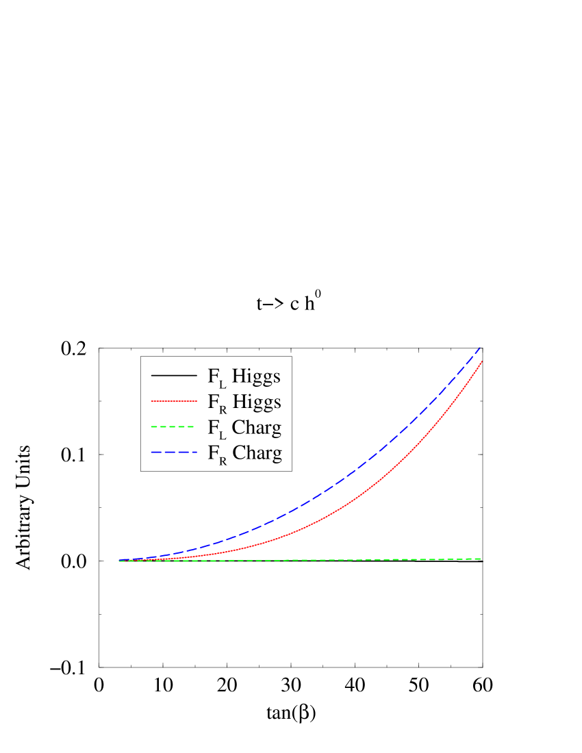
Figure 5.4: Different form factors (5.6) for the channel $t\rightarrow c\,h^{0}$ as a function of $\tan\beta$, with the typical set of inputs of eq.(5.3.2).

In Fig. 5.4 we have plotted the different form factors of (5.6) as a function of $\tan\beta$ for the channel with the lightest scalar Higgs ($h^{0}$). We can see that the contributions from the Higgs sector and the contributions from the chargino sector are of the same order. It turns out that they can be either of the same sign, or of opposite sign. The chosen negative value for $A_{b}$ is to make the two contributions of the same sign. It is also clear that in both cases $F_{R}\gg F_{L}$. This can be easily understood by looking at the interaction Lagrangians involving higgsino-sbottom-charm and Higgs-bottom-charm:

$${\cal L}_{\tilde{h}\,\tilde{b}\,c} = -g\,V_{cb}\,\bar{c}\left({R_{1a}^{(b)}\,\lambda_{c}}\,P_{L}+{R_{2a}^{(b)}\,\lambda_{b}}\,P_{R}\right)\chi^{+}\tilde{b}_{a}+\mbox{ h.c.}$$

$${\cal L}_{H\,b\,c} = \frac{g}{\sqrt{2}M_{W}}V_{cb}\,\bar{c}\left({m_{c}\,\cot\beta}\,P_{L}+{m_{b}\,\tan\beta}\,P_{R}\right)\,b\,H^{+}+\mbox{ h.c.}\,\,\,,$$ (5.18)

we can see that in both of them the contribution to the right-handed form factor will be enhanced by the Yukawa coupling of the bottom quark, compared with the charm Yukawa coupling that will contribute to the left-handed form factor. On the other hand we have checked that the inclusion of the first two generations of quarks and squarks only has an effect of a few percent on the total result.

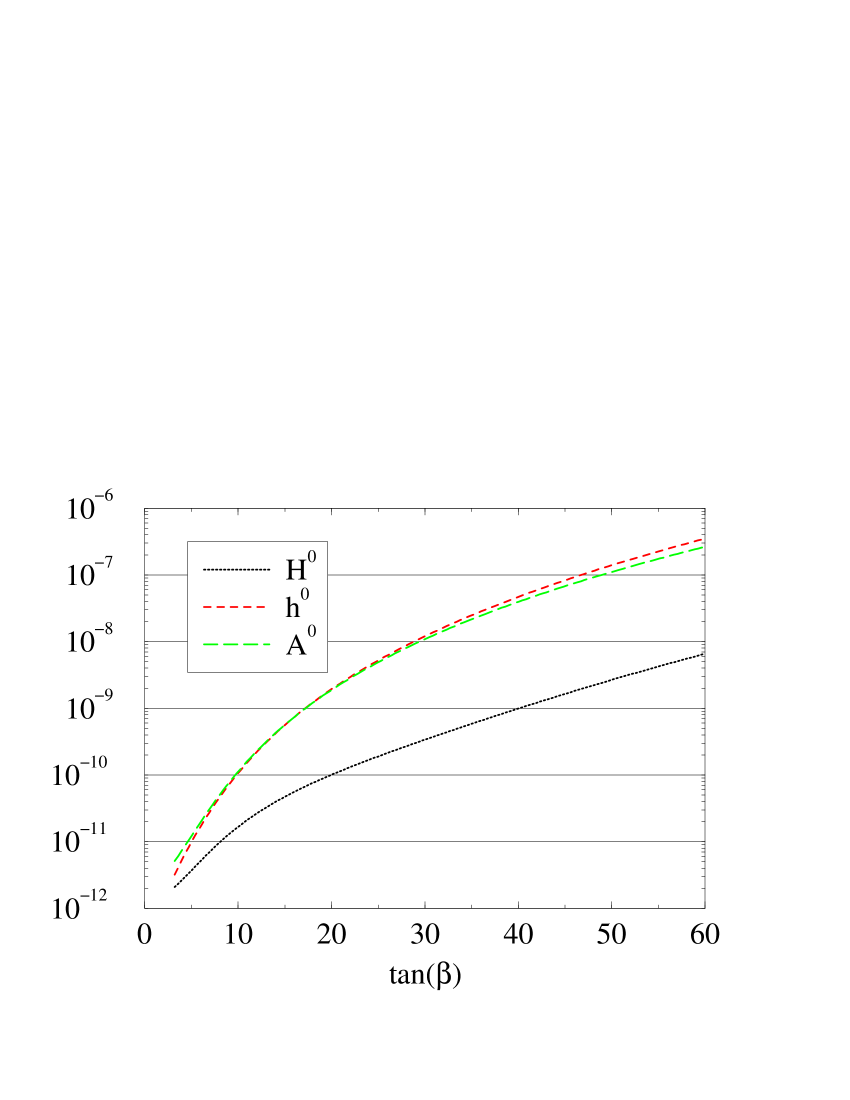
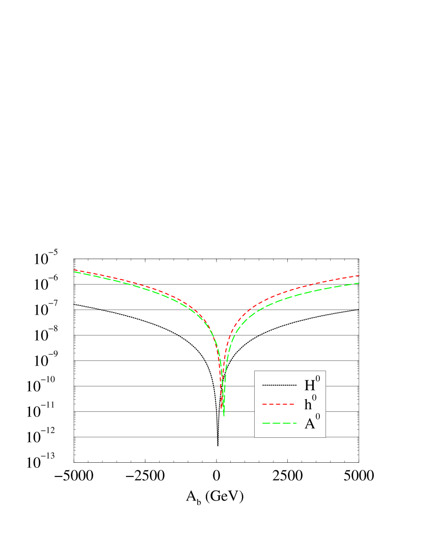
(a)	(b)
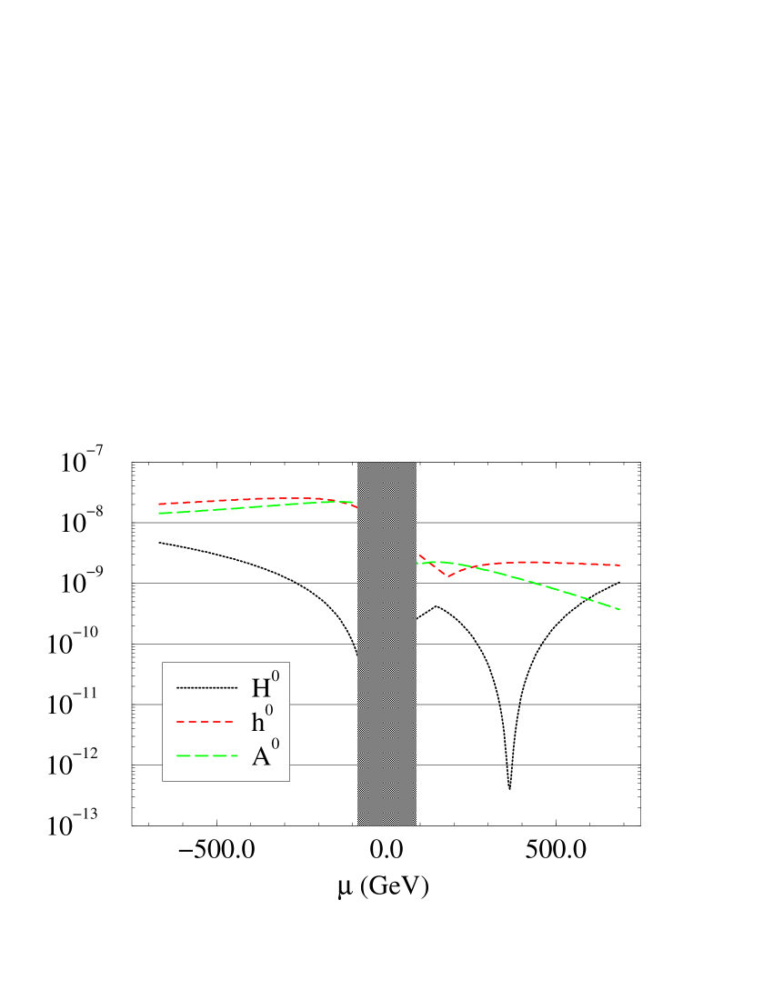
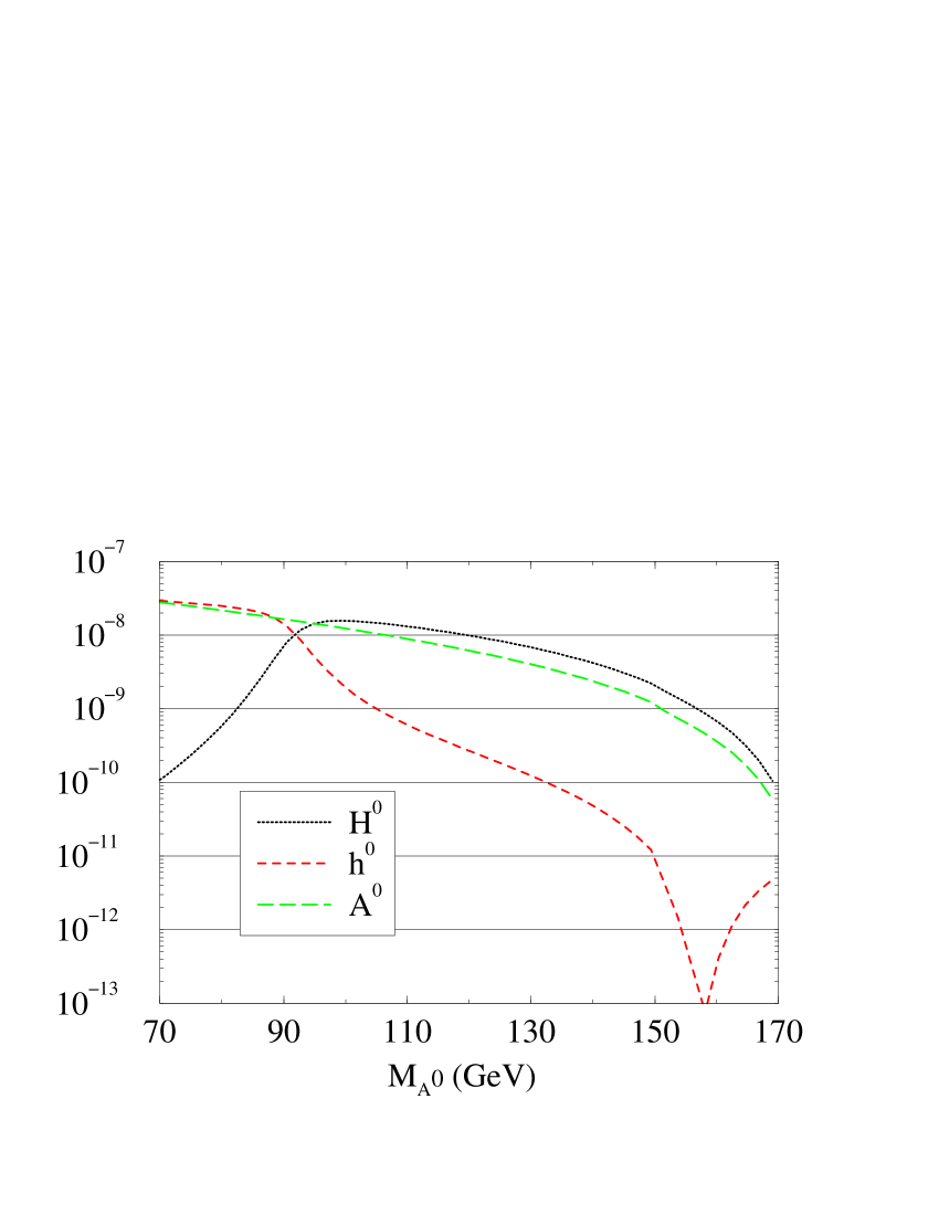
(c)	(d)

Figure 5.5: Evolution of the ratio (5.8) with (a) $\tan\beta$, (b) the trilinear coupling $A_{b}$, (c) the higgsino mass parameter $\mu$, and (d) the pseudoscalar Higgs mass $M_{A^{0}}$. The rest of inputs are given in eq.(5.3.2).

In Fig. 5.5 we can see the evolution of the ratio (5.8) with various parameters of the MSSM, by taking into account only the electroweak contributions. The growing of the width with $\tan\beta$ (Fig. 5.5 (a)) shows that the bottom Yukawa coupling plays a central role in these contributions. The evolution with the trilinear coupling $A_{b}$ and the higgsino mass parameter $\mu$ –the two parameters that appear in the trilinear coupling $\tilde{b}_{L}\,\tilde{b}_{R}\,h$– displayed in Figs. 5.5 (b) and (c) shows that these parameters can enhance the width some orders of magnitude. We have artificially let $A_{b}$ grow up to large scales (that are not allowed if one wants that squarks do not develop vacuum expectation values) in order to emphasize the dependence on $A_{b}$. The various spikes in these figures reflect the points where the form factors change sign, whereas the shaded region in Fig. 5.5 (c) reflects the exclusion region of $\mu$ by present LEP bounds on the chargino mass.

In all these figures the ratio (5.8) is smaller for the heaviest scalar Higgs ($H^{0}$) because with the parameters (5.3.2) the CP-even Higgs mixing angle $\alpha$ is near $-\pi/2$, so making the couplings of $H^{0}$ with down quarks and squarks much weaker, but in fig. 5.5 (d) it can be seen that when the pseudoscalar Higgs mass grows (and this shifts $\alpha$ far away from $-\pi/2$) the two scalar Higgs bosons change roles.

We conclude that the typical value of the ratio (5.8), at large $\tan\beta\mbox{ \raisebox{-4.0pt}{${\stackrel{{\scriptstyle\textstyle<}}{{\sim}}}$} }50$ and for a SUSY spectrum around $200\mbox{ GeV}$, is

$$B^{\rm SUSY-EW}(t\rightarrow c\,h)\simeq{\cal O}(10^{-8})\,\,\,.$$ (5.19)

In favorable regions of the parameter space it can grow up to $10^{-7}$. The maximum value is found to be in the ballpark of several $10^{-6}$, for sufficiently large $A_{b}$. This is an improvement of the previous result[206], specially in the $A^{0}$ channel, by two orders of magnitude.

5.4 SUSY-QCD contributions

The gluino-mediated supersymmetric strong interactions in the MSSM  can also produce FCNC processes. This occurs when the squark mass matrix does not diagonalize with the same matrix as the one for the quarks. We introduce then intergenerational mass terms for the squarks, but in order to prevent the number of parameters from being too large, we have allowed (symmetric) mixing mass terms only for the left-handed squarks. This simplification is often used in the MSSM, and is justified by RGE analysis[211].

The mixing terms are introduced through the parameters $\delta_{ij}$ defined as

$$(M^{2}_{LL})_{ij}=m_{ij}^{2}\equiv\delta_{ij}\,m_{i}\,m_{j}\,\,,$$ (5.20)

where $m_{i}$ is the mass of the left-handed $i$ squark, and $m^{2}_{ij}$ is the mixing mass matrix element between the generations $i$ and $j$. Thus we must diagonalize two $6\times 6$ mass matrices in order to obtain the mass-eigenstates squark fields. Following a notation similar to the standard one we introduce the mixing matrices as follows (Cf. Sec. 2.4.3)

$$\tilde{q}^{\prime}_{\alpha} = \sum_{\beta}R^{(q)}_{\alpha\beta}\tilde{q}_{\beta}$$

$$R^{(q)\dagger}{\cal M}^{2}_{\tilde{q}}R = {\cal M}_{\tilde{q}D}^{2}={\rm diag}\{m^{2}_{\tilde{q}_{1}},\ldots,m^{2}_{\tilde{q}_{6}}\}\,\,,\,\,q\equiv u,\,d\,\,,$$ (5.21)

where ${\cal M}^{2}_{(\tilde{u},\tilde{d})}$ is the $6\times 6$ square mass matrix for up-type (or down-type) squarks in the EW  basis, with indices $\alpha=1,2,3,\ldots,6\equiv\tilde{u}_{L},\tilde{u}_{R},\tilde{c}_{L},\ldots,\tilde{t}_{R}$ for up-type squarks, and an equivalent choice for down-type squarks. In this study we are only interested in the up-type quarks-squarks system, so we will drop out the $(q)$ super-index in the forthcoming expressions. The rotation matrix $R$ introduces gluino mediated tree-level FCNC  between quarks and squarks, the corresponding interaction Lagrangian can be deduced using the very same formalism of the “ordinary” SUSY-QCD (2.34) interactions, but using the more general rotation matrix (5.4),

$${\cal L}_{\rm SUSY-QCD} = -\frac{g_{s}}{\sqrt{2}}\,\bar{\psi}_{c}^{\tilde{g}}\left[R_{5\alpha}^{*}\,P_{L}-R_{6\alpha}^{*}\,P_{R}\right]\tilde{q}^{*}_{\alpha,i}\,\lambda_{ij}^{c}\,t_{j}$$ (5.22)

$$- \frac{g_{s}}{\sqrt{2}}\,\bar{\psi}_{c}^{\tilde{g}}\left[R_{3\alpha}^{*}\,P_{L}-R_{4\alpha}^{*}\,P_{R}\right]\tilde{q}^{*}_{\alpha,i}\,\lambda_{ij}^{c}\,c_{j}$$

$$- \frac{g_{s}}{\sqrt{2}}\,\bar{\psi}_{c}^{\tilde{g}}\left[R_{1\alpha}^{*}\,P_{L}-R_{2\alpha}^{*}\,P_{R}\right]\tilde{q}^{*}_{\alpha,i}\,\lambda_{ij}^{c}\,u_{j}\,\,.$$

5.4.1 Vertex and self-energy functions

Using the Lagrangian (5.22) one can find the SUSY-QCD  one-loop contributions to the process under study, which Feynman diagrams are depicted in Figs. 5.6 and 5.7. The vertex diagram contributions to the form factors (5.6) in Fig. 5.6 can be written as

(0,15)(0,5)(200,80) thin i1 o2,o1 fermion,label.side=left,label=$t$i1,v1 fermion,label.side=left,label=             $c$v2,o1 dashes,label.side=left,label=             $h$v3,o2 fermion,label=$\tilde{g}$v1,v2 scalar,label=$\tilde{u}_{\beta}$,label.side=rightv3,v2 scalar,label=$\tilde{u}_{\alpha}$,label.side=rightv1,v3 .6w,1hv2 .6w,0v3 .3w,.5hv1

Figure 5.6: One-loop SUSY-QCD  vertex diagram contributing to the decay $t\rightarrow c\,h$. $\tilde{u}_{\{\alpha,\beta\}}$ represent mass-eigenstate up type squarks of any generation.

(0,10)(0,10)(140,70) thin i1 o1 fermion,label=$t$,label.side=lefti1,v1 scalar,label=$\tilde{u}_{\alpha}$,right,tension=0.5v1,v2 fermion,label=$\tilde{g}$,left,tension=0.5v1,v2 fermion,label=$c$,label.side=leftv2,o1

Figure 5.7: One-loop SUSY-QCD  diagrams contributing to mixed $t-c$ self-energy. $\tilde{u}_{\alpha}$ represent mass-eigenstate up type squarks of any generation.

$$F_{L} = N\,\left[m_{t}\,R_{4\beta}\,R_{6\alpha}^{*}\,(C_{11}-C_{12})\right.$$

$$\left.+m_{c}\,R_{3\beta}\,R_{5\alpha}^{*}\,C_{12}+m_{\tilde{g}}\,R_{4\beta}\,R_{5\alpha}^{*}C_{0}\right]$$

$$F_{R} = F_{L}\left(3\leftrightarrow 4\,\,,\,\,5\leftrightarrow 6\right)$$

$$N = i\,8\,\pi\,\alpha_{s}\,C_{F}\,R_{i\beta}^{*}\,G_{ij}^{r}\,R_{j\alpha}$$

$$C_{*} = C_{*}(-k,p^{\prime},m_{\tilde{g}},m_{\tilde{u}_{\alpha}},m_{\tilde{u}_{\beta}})\,\,,$$ (5.23)

where $G_{ij}^{r}$ is the Feynman rule of $\Phi^{0}_{r}\rightarrow\tilde{u}_{i}^{\prime}\tilde{u}_{j}^{\prime*}$ divided by $-ig$, with $\tilde{u}^{\prime}_{1,2}$ the electroweak eigenstates of up-type squarks[39, 71].

The one-loop mixing self-energy in Fig. 5.7 takes the following form

$$\Sigma_{L}(k^{2}) = -i\,2\,\pi\,\alpha_{s}\,C_{F}\,R_{3\alpha}\,R_{5\alpha}^{*}\,B_{1}(-k,m_{\tilde{g}},m_{\tilde{u}_{\alpha}})$$

$$\Sigma_{R}(k^{2}) = -i\,2\,\pi\,\alpha_{s}\,C_{F}\,R_{4\alpha}\,R_{6\alpha}^{*}\,B_{1}(-k,m_{\tilde{g}},m_{\tilde{u}_{\alpha}})$$

$$m_{t}\,\Sigma_{Ls}(k^{2}) = -i\,2\,\pi\,\alpha_{s}\,C_{F}\,m_{\tilde{g}}\,R_{4\alpha}\,R_{5\alpha}^{*}\,B_{0}(-k,m_{\tilde{g}},m_{\tilde{u}_{\alpha}})$$

$$m_{t}\,\Sigma_{Rs}(k^{2}) = -i\,2\,\pi\,\alpha_{s}\,C_{F}\,m_{\tilde{g}}\,R_{3\alpha}\,R_{6\alpha}^{*}\,B_{0}(-k,m_{\tilde{g}},m_{\tilde{u}_{\alpha}})$$ (5.24)

where $C_{F}=(N_{c}^{2}-1)/2N_{c}=4/3$ is a well known colour factor. Now we can introduce these expressions in (5.5) and (5.6) to obtain the relevant branching ratio under study (5.8).

5.4.2 Numerical Analysis

For the numerical analysis we must provide as input parameters, apart from that of the Higgs sector, the various squark masses and mixings, i.e. the $\delta$ parameters of (5.20). These $\delta$ parameters are constrained by low energy data on FCNC[212, 213]. The bounds have been computed using some approximations, so they must be taken as order of magnitude limits. We use the following bounds[212, 213]

$$|\delta_{12}| < .1\,\sqrt{m_{\tilde{u}}\,m_{\tilde{c}}}/{500\mbox{ GeV}}$$

$$|\delta_{13}| < .098\,\sqrt{m_{\tilde{u}}\,m_{\tilde{t}}}/{500\mbox{ GeV}}$$

$$|\delta_{23}| < 8.2\,m_{\tilde{c}}\,m_{\tilde{t}}/{(500\mbox{ GeV})^{2}}\,\,\,.$$ (5.25)

For the various parameters that are common to the EW  analysis we use the same input parameters (5.3.2) to which we must add the specific parameters of the SUSY-QCD  sector, namely

$$m_{\tilde{g}} = 150\mbox{ GeV}$$

$$\delta = \left(\begin{array}[]{ccc}0&0.03&0.03\\ &0&0.6\\ &&0\end{array}\right)\,\,\,.$$ (5.29)

A comment is in order for the present set of inputs: we have introduced in (5.3.2) the lightest stop mass as an input, and this stop is mostly a $\tilde{t}_{R}$. However, in this new parametrization we introduce this mass as the lightest $\tilde{u}_{\alpha}$ mass, which will be mostly a $\tilde{t}_{R}$.

Again the largest contribution comes from the right-handed form factor of (5.6), but this is only because we have chosen not to introduce mixing between right-handed squarks.

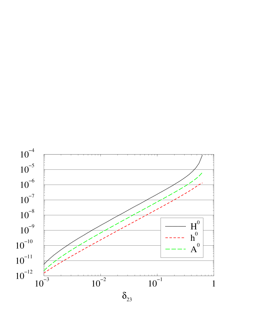
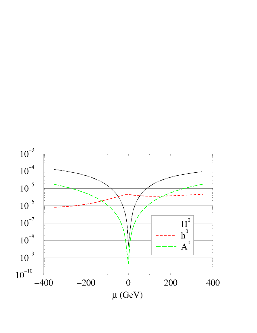
(a)	(b)
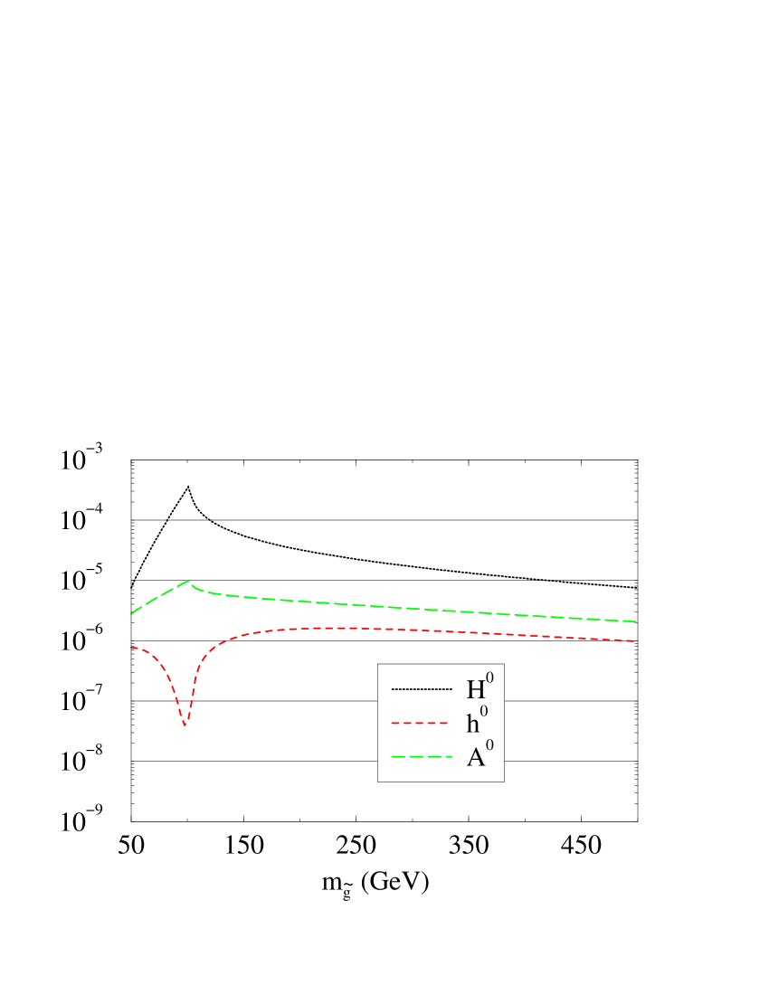
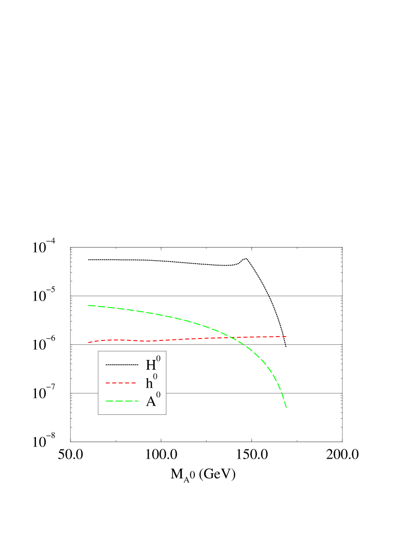
(c)	(d)

Figure 5.8: Evolution of the ratio (5.8) with (a) the mixing parameter between the 2nd and 3rd squark generations $\delta_{23}$, (b) the higgsino mass parameter $\mu$, (c) the gluino mass $m_{\tilde{g}}$, and (d) the pseudoscalar Higgs mass $M_{A^{0}}$, the rest of inputs are given in eqs.(5.3.2) and (5.4.2).

We have plotted the evolution of the ratio (5.8) with some parameters of the MSSM in Fig. 5.8. As can be easily guessed, the most important parameter for these contributions is the mixing mass parameter between the 2nd and 3rd generation of left-handed squarks, the less restricted one of the three (eq. (5.4.2)). In Fig. 5.8 (a) it is shown that changing $\delta_{23}$ by 3 orders of magnitude, the ratio (5.8) can increase by 7 orders of magnitude! We can see in Fig. 5.8 (b) that the $\mu$ parameter also plays an important role, like in the electroweak contributions (Fig. 5.5 (c)), and for the same reasons, bringing the ratio (5.8) up to values of $10^{-4}$. Notice that the central region of $|\mu|\mbox{ \raisebox{-4.0pt}{${\stackrel{{\scriptstyle\textstyle<}}{{\sim}}}$} }90\mbox{ GeV}$ is excluded by present LEP bounds on the chargino mass.

The evolution with the gluino mass (Fig. 5.8 (c)) is asymptotically quite stable, showing a slow decoupling. Finally in Fig. 5.8 (d) we have plotted the evolution with the pseudoscalar Higgs mass, it is also quite stable, until near the kinematic limit for $A^{0}$ and $H^{0}$.

We conclude that the typical value of the SUSY-QCD contributions to (5.8), with a SUSY spectrum around $200\mbox{ GeV}$, is

$$B^{\rm SUSY-QCD}(t\rightarrow c\,h)\simeq{\cal O}\,(10^{-5})\,\,\,,$$ (5.30)

but in favourable regions of the parameter space (i.e.  large $\mu$, or relatively light gluino) it can easily reach values of $10^{-4}$. The upper bound is at several $10^{-4}$. This is 1-2 orders of magnitude larger than the previous estimate[206].

5.5 Conclusions

We have computed the SUSY-EW, Higgs, and SUSY-QCD contributions to the FCNC  top quark decay $t\rightarrow c\,h$ ($h=h^{0},H^{0},A^{0}$) in the MSSM, using a mass spectrum motivated, but not fully restricted, by model building and Renormalization Group Equations.

We have found that with a SUSY mass spectrum around $200\mbox{ GeV}$, which is well above present bounds, the different contributions to this decay are typically of the order

$$B^{\rm SUSY-EW}(t\rightarrow c\,h) \simeq 10^{-8}\,\,,$$

$$B^{\rm SUSY-QCD}(t\rightarrow c\,h) \simeq 10^{-5}-10^{-4}\,\,\,.$$ (5.31)

The difference of at least two orders of magnitude between the two contributions makes unnecessary to compute the interference between the two contributions, but if the limits on $\delta_{23}$ (eq. (5.4.2)) improve, it should be necessary to make the full computation.

The results (5.5) are an improvement of the previous estimate [206], specially in the $A^{0}$ channel, thanks to the inclusion of the $\tilde{q}_{L}\,\tilde{q}_{R}\,h$ vertex.

It would probably be difficult that this decay can be measured either at the Tevatron, or at the NLC, but there exists a possibility for LHC. As an example to assess the discovery reach of these accelerators the FCNC  top quark decays into a vector boson are[214]

$${\rm\bf LHC:} B(t\rightarrow c\,V) >5\times 10^{-5}\,\,,$$

$${\rm\bf NLC:} B(t\rightarrow c\,V) >10^{-3}-10^{-4}\,\,\,,$$ (5.32)

where the lack of sensitivity of the NLC is due to the lower luminosity. So, if the discovery reach for FCNC  Higgs processes are not very different from that of the gauge bosons, there is a possibility to measure this decay channel at the LHC even if SUSY  particles are not seen at the LEPII.

Chapter 6 One-loop corrections to scalar quark decays

6.1 Introduction

Sparticles not much heavier than a few hundred GeV could be produced in significant numbers already at the Tevatron. For instance, selectron production was advocated in Ref.[25] to explain a purported non-SM event in the Collider Detector at Fermilab (CDF). Subsequently, in Refs.[132, 159] it was argued that half of the top quarks at the Tevatron might come from gluino decays into top and stop, $\tilde{g}\rightarrow t\,\bar{\tilde{t}}_{1}$. Similarly, as discussed in the introduction, we may envision the possibility that sbottom squarks are pair produced by the usual Drell-Yan mechanism and then decay into top quark and charginos: $\tilde{b}_{a}\rightarrow t\,\chi^{-}_{i}$. Indeed, this would be the leading two-body decay if gluinos are heavy enough that the strong decay mode $\tilde{b}_{a}\rightarrow\tilde{g}\,b$ is kinematically blocked up. The observed cross-section would then be the one of eq. (1.4). We shall assume thorough present study that gluinos are much heavier than squarks, so that their contribution to this cross-section through $q\,\bar{q}\rightarrow\tilde{g}\,\tilde{g}$ followed by $\tilde{g}\rightarrow t\,\bar{\tilde{t}}_{1}$ is negligible. We could have non-SM  top quark decay modes, such as e.g. $t\rightarrow\tilde{t}_{a}\,\chi^{0}_{\alpha}$ [132, 159] and $t\rightarrow H^{+}\,b$ [51, 50], that could serve, pictorially, as a “sinkhole” to compensate (at least in part) for the unseen source of extra top quarks produced at the Tevatron from sbottom pair production (Cf. eq.(1.4)). As stated in section 4.2 one cannot exclude that then non-SM branching ratio $BR(t\rightarrow\mbox{``new''})$, could be as big as the SM one, i.e. $\sim 50\%$.

If $\tan\beta$ is large and there exists a relatively light chargino with a non-negligible higgsino component, the alternative mechanism suggested in eq.(1.4) could be a rather efficient non-SM  source of top quarks that could compensate for the depletion in the SM  branching ratio.

While the squark production cross-section has already received some attention in the literature at the level of NLO radiative corrections  [218, 219, 220], an accurate treatment of the decay mechanisms is also very important to provide a solid basis for experimental analysis of the top quark production in the MSSM. Thus in this chapter we consider the computation of the QCD  and leading supersymmetric electroweak (SUSY-EW) quantum effects on $\tilde{b}_{a}\rightarrow t\,\chi^{-}_{i}$, namely the ones induced by potentially large Yukawa-couplings from the top and bottom quarks (2.18).

6.2 Vertex renormalization

The one-loop Lagrangian of the $\tilde{b}\,t\,\chi^{-}$ interaction follows after substituting the one-loop counterterms, that of $\tilde{b}$, $t$, and $\chi^{-}$  from chapter 3 into the bare Lagrangian (2.32),

$${\cal L}^{0}_{\chi^{-}\,t\,\tilde{b}}=-g\,\tilde{b}^{*}_{a}\bar{\chi}^{+}_{i}\left[\left(A_{+ai}^{(b)}+\delta C^{ai}_{+}\right)P_{L}+\epsilon_{i}\left(A_{-ai}^{(b)}+\delta C^{ai}_{-}\right)P_{R}\right]t+{\rm h.c.}\,,$$ (6.1)

with

$$\delta C^{ai}_{+} = A_{+ai}^{(b)}\left(\frac{\delta g}{g}+\frac{1}{2}\delta Z^{a}+\frac{1}{2}\delta Z_{R}^{i}+\frac{1}{2}\delta Z_{L}^{t}\right)+\delta A_{+ai}^{(b)}+\delta Z^{ba}A_{+ai}^{(b)}\,,$$

$$\delta C^{ai}_{-} = A_{-ai}^{(b)}\left(\frac{\delta g}{g}+\frac{1}{2}\delta Z^{a}+\frac{1}{2}\delta Z_{L}^{i}+\frac{1}{2}\delta Z_{R}^{t}\right)+\delta A_{-ai}^{(b)}+\delta Z^{ba}A_{-ai}^{(b)}\,.$$ (6.2)

where we have introduced the shortcuts

$$\delta A_{+ai}^{(b)} = \delta R_{1a}^{(b)*}\,V_{i1}^{*}-(\delta R_{2a}^{(b)*}\,\lambda_{b}+R_{2a}^{(b)*}\,\delta\lambda_{b})\,V_{i2}^{*}$$

$$\delta A_{-ai}^{(b)} = -(\delta R_{1a}^{(b)*}\,\lambda_{t}+R_{1a}^{(b)*}\,\delta\lambda_{t})\,U_{i2}\,.$$ (6.3)

We have not introduced the mixing self-energies between the two charginos ($\delta Z^{ij}$) as they do not contribute. In the case of the QCD corrections the chargino gets no correction, whereas the Yukawa coupling approximation implies no mixing between charginos (see section 6.5). For the very same reasons we do not show the shift that the chargino mixing matrices $U$ and $V$ would develop at one-loop.

The full structure of the four on-shell renormalized decay amplitudes for $\tilde{b}_{a}\rightarrow t\,\chi^{-}_{i}\,(a=1,2;i=1,2)$ follows from the previous Lagrangian after including the contributions from the (LH and RH) one-loop vertex form factors $F_{L,R}^{ai}$:

$$i\,T(\tilde{b}_{a}\rightarrow t\,\chi^{-}_{i})=i\,g\,\bar{u}_{t}\,\left[\epsilon_{i}\left(A_{-ai}^{(b)}+\Lambda_{L}^{ai}\right)P_{L}+\left(A_{+ai}^{(b)}+\Lambda_{R}^{ai}\right)P_{R}\right]\,v_{i}$$ (6.4)

where

$$\Lambda_{L}^{ai}=\delta C_{-}^{ai}+\epsilon_{i}\,F_{L}^{ai}\,,\ \ \ \ \ \Lambda_{R}^{ai}=\delta C_{+}^{ai}+F_{R}^{ai}\,.$$ (6.5)

(0,10)(0,10)(140,70) thin i1 o2,o1 $t(p)$o1 $\chi^{-}_{i}(p^{\prime})$o2 scalar,label=$\tilde{b}_{a}(k)$,label.side=lefti1,v1 fermionv1,o1 fermiono2,v1

Figure 6.1: Tree-level Feynman diagram of the process $\tilde{b}_{a}\rightarrow t\chi^{-}_{i}$

Let now $\Gamma_{0}^{ai}$ be the tree-level partial width of the decay $\tilde{b}_{a}\rightarrow t\,\chi^{-}_{i}$, the only Feynman diagram contributing to this process in depicted in figure 6.1, and from the Lagrangian (2.32) we can obtain:

$$\Gamma_{0}^{ai} = \frac{g^{2}}{16\,\pi\,m_{\tilde{b}_{a}}^{3}}\,\lambda^{1/2}(a,i,t)\,\left\{\left[(A_{+ai}^{(b)})^{2}+(A_{-ai}^{(b)})^{2}\right]\,(m_{\tilde{b}_{a}}^{2}-M^{2}_{i}-m_{t}^{2})\right.$$ (6.6)

$$\left.\phantom{\left[(A_{+ai}^{(b)})^{2}+(A_{-ai}^{(b)})^{2}\right]}-4\,A_{+ai}^{(b)}\,A_{-ai}^{(b)}\,m_{t}\,\epsilon_{i}\,M_{i}\right\}\,,$$

with $\lambda(a,i,t)\equiv\lambda(m_{\tilde{b}_{a}}^{2},M^{2}_{i},m_{t}^{2})$ the usual Källen function for the given arguments. The quantum correction to $\Gamma_{0}^{ai}$ can be described in terms of the quantities $\delta^{ai}=(\Gamma^{ai}-\Gamma_{0}^{ai})/\Gamma_{0}^{ai}$, where $\Gamma^{ai}$ is the corresponding one-loop corrected width. From the previous formulae, $\delta^{ai}$ can be worked out as follows:

$$\delta^{ai}=\frac{2\left(m_{\tilde{b}_{a}}^{2}-M^{2}_{i}-m_{t}^{2}\right)\left(A_{-ai}^{(b)}\,\Lambda_{L}^{ai}+A_{+ai}^{(b)}\,\Lambda_{R}^{ai}\right)-4\,m_{t}\,\epsilon_{i}\,M_{i}\,(A_{-ai}^{(b)}\Lambda_{R}^{ai}+A_{+ai}^{(b)}\,\Lambda_{L}^{ai})}{\left[(A_{+ai}^{(b)})^{2}+(A_{-ai}^{(b)})^{2}\right]\left(m_{\tilde{b}_{a}}^{2}-M^{2}_{i}-m_{t}^{2}\right)-4\,A_{+ai}^{(b)}\,A_{-ai}^{(b)}\,m_{t}\,\epsilon_{i}\,M_{i}}\,.$$ (6.7)

As mentioned in chapter 3 we use an on-shell renormalization procedure, so the input parameters for the sbottom sector will be the masses as well as the mixing angle

$$(m_{\tilde{b}_{1}},m_{\tilde{b}_{2}},\theta_{\tilde{b}})\,,$$ (6.8)

whereas for the stop sector we just have in addition

$$(m_{\tilde{t}_{1}},\theta_{\tilde{t}})\,\,,$$ (6.9)

since by $SU(2)_{L}$ gauge invariance the value of the other stop mass $m_{\tilde{t}_{2}}$ is already determined. Of course, $\tan\beta$ and the SUSY  Higgs mixing parameter $\mu$ are also additional independent inputs for our calculation. Similarly, the sbottom and stop trilinear terms $A_{b}$ and $A_{t}$ are fixed by the previous parameters as follows:

$$A_{b}=\mu\,\tan\beta+{m_{\tilde{b}_{2}}^{2}-m_{\tilde{b}_{1}}^{2}\over 2\,m_{b}}\,\sin{2\,\theta_{\tilde{b}}}\,;\ \ \ \ A_{t}=\mu\,\cot\beta+{m_{\tilde{t}_{2}}^{2}-m_{\tilde{t}_{1}}^{2}\over 2\,m_{t}}\,\sin{2\,\theta_{\tilde{t}}}\,,$$ (6.10)

of course the $\tilde{t}_{2}$ mass, as well as the $A$ parameters form eq. (6.10) will receive radiative corrections, but these would be second order corrections to our process. We must be careful with the value of these $A$ parameters, as explained in section 2.4.3 they are bounded by the condition of colour-breaking vacua (2.23), as well as the condition of perturbativity of the Higgs-squark-squark couplings. These bounds will translate into a forbidden region in the parameter space defined by (6.8) and (6.9). As the conditions mentioned above are fairly qualitative we will present our results in all of the parameter space, but at the same time we will single out the regions where the conditions (2.23) are fulfilled.

6.3 Tree-level results

In this section we make a simple tree-level analysis of the MSSM  parameter space, trying to single out the regions where the process under study should be interesting. In order to achieve this we focus on the sbottom decay itself, but also on the sbottom production mechanism and on the top quark decay.

As we are interested in the effects that this decay could have at the Tevatron we should use relatively light sbottom masses (a few hundred GeV). On the other hand, as this processes would imply a growing of the top quark production cross-section (1.4), it is necessary a mechanism that would keep this cross-section at its measured value, so the top quark should have available non-standard decay channels, e.g.  $t\rightarrow H^{+}\,b$, thus the charged Higgs mass should comply with

$$M_{H^{\pm}}<m_{t}-m_{b}\,\,,$$ (6.11)

another possibility could be the supersymmetric channel $t\rightarrow\tilde{t}_{1}\,\chi^{0}_{1}$, however this latter channel cannot be under control, for example, in the Yukawa approximation performed in section 6.5 it is necessarily blocked up.

It is clear that the radiative corrections to the process $\tilde{b}_{a}\rightarrow t\,\chi^{-}_{i}$ will only be interesting in the region where it also has a large tree-level branching ratio. Apart from the already stated gluino decay channel there are also other channels ($\tilde{b}_{a}\rightarrow b\,\chi^{0}_{\alpha}$, $\tilde{b}_{2}\rightarrow\tilde{b}_{1}h^{0}$, …) that will contribute to this decay width. To have an appreciable branching ratio $\tilde{b}_{a}\rightarrow t\,\chi^{-}_{i}$ we start out supposing that the gluino is much heavier than the squarks

$$m_{\tilde{g}}>m_{\tilde{b}_{a}}\,\,\,(a=1,\,2)\,\,,$$ (6.12)

neutralino masses, on the other hand, are related to chargino ones, so no additional conditions can be put on this side. Let us define the branching ratio in which we are interested:

$$BR_{0}(\tilde{b}_{a}\rightarrow t\,\chi^{-}_{1}) = {\Gamma_{0}(\tilde{b}_{a}\rightarrow\chi^{-}_{1}\,t)\over\Gamma_{0}^{T}(\tilde{b}_{a})}\,\,,$$

$$\Gamma_{0}^{T}(\tilde{b}_{a}) = \sum_{\alpha}\Gamma_{0}(\tilde{b}_{a}\rightarrow b\,\chi^{0}_{\alpha})+\Gamma_{0}(\tilde{b}_{a}\rightarrow t\,\chi^{-}_{1})+\Gamma_{0}(\tilde{b}_{a}\rightarrow\tilde{t}_{1}\,H^{-})$$ (6.13)

$$+\sum_{i}\,\Gamma_{0}(\tilde{b}_{a}\rightarrow\tilde{b}_{b}\,\Phi^{0}_{i})\,,$$

(where $\Phi_{i}^{0}=h^{0},H^{0},A^{0}$). To maximize this branching ratio we should work in an scenario where the lightest chargino is higgsino-dominated, and $\tan\beta$  should have a low-moderate value, if $\tan\beta$  is large ($\mbox{ \raisebox{-4.0pt}{${\stackrel{{\scriptstyle\textstyle>}}{{\sim}}}$} }40$) then $\Gamma_{0}^{T}$ is dominated by the neutral higgsino contribution (first summand of expr. (6.13)).

In figure 6.2 we have plot the value of the branching ratio (6.13) as a function of $\tan\beta$, $m_{\tilde{b}_{1}}$ and $\theta_{\tilde{b}}$ for given values of the other parameters. From the figure it is clear that low $\tan\beta$  enhances this branching ratio. From now on we will concentrate in the region of $\tan\beta\simeq 20$, with this typical value the branching ratio still has an appreciable branching ratio, whereas the electroweak corrections can be enhanced by means of the bottom Yukawa coupling (2.18). In Fig. 6.2(b) we can see the opening of the Higgs channels, namely $\tilde{b}_{2}\rightarrow\tilde{b}_{1}\,\Phi_{1}^{0}$ (at the left end of the figure) and $\tilde{b}_{1}\rightarrow\tilde{t}_{1}\,H^{-}$ (at its right end), it is clear that when this channels are open they tend to take the branching ratio (6.13) to undetectable values. This large value of the Higgs decay width is due to the fact that in this regions the $A$ parameters (6.10) acquire large values. Of course one could fix the input parameters (6.8) in such a way that $A_{\{t,b\}}$ are small in one of this regions (say at $m_{\tilde{b}_{1}}$ light), but at the price of making them large at its central value and even larger at the other end. This effect is also seen in Fig. 6.2(c), as the $A$ parameters are related to the angle trough (6.10). Another possibility would be to push the Higgs masses to a high value, which would be in contradiction with the requirement (6.11). Note that the allowed range of $\theta_{\tilde{b}}$ is rather narrow, so that the physical sbottom masses basically coincide with the LH and RH electroweak eigenstates.

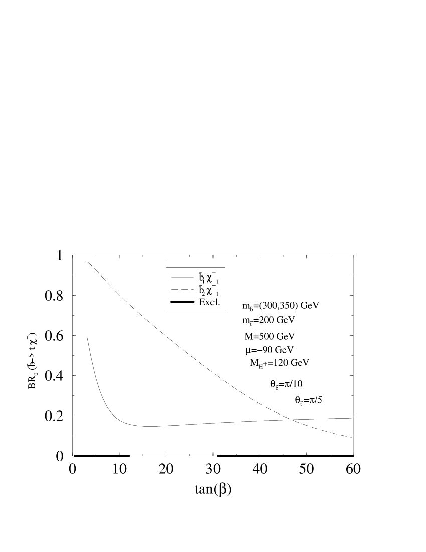
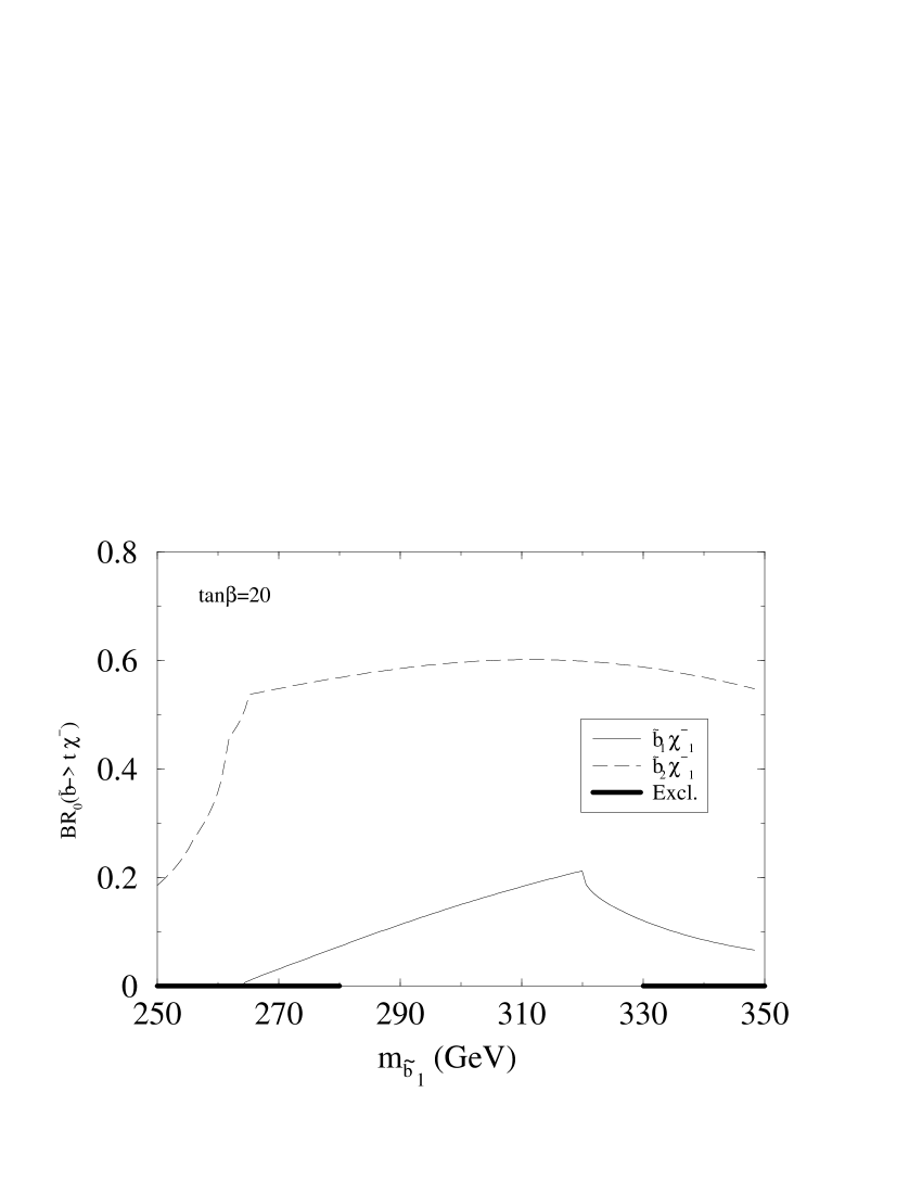
(a)	(b)
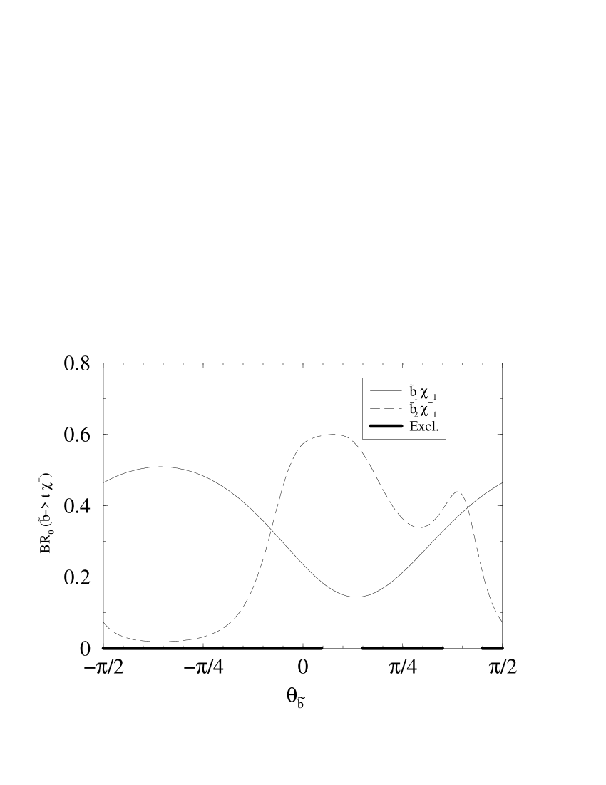
(c)

Figure 6.2: (a) The branching ratio of  $\tilde{b}_{a}\rightarrow\chi_{1}^{-}\,t$  as a function of $\tan\beta$ for the various decays $a=1,2$ with $m_{\tilde{b}_{1}}<m_{\tilde{b}_{2}}$; (b) As in (a), but as a function of $m_{\tilde{b}_{1}}$; (c) As in (a), but as a function of $\theta_{\tilde{b}}$. The marked parts of the abscissa in both figures are excluded by the condition (2.23). The fixed parameters for (a) and (b) are given in the frame.

6.4 QCD  corrections

The first step to the computation of the quantum effects on $\tilde{b}_{a}\rightarrow t\,\chi^{-}_{i}$ is to compute the QCD  corrections, as they are expected to be larger than the EW  ones.

The evaluation of the one-loop QCD  corrections to the decay $\tilde{b}_{a}\rightarrow t\,\chi^{-}_{i}$ comprise the computation of the gluon and the gluino mediated diagrams. These corrections were computed in [57, 58], however we use slightly different renormalization conditions, and we present our numerical results in a completely different way. We have checked analytically our results with that of [57, 58], and also numerically in the case of [57].

In this process it is not possible to separate between the gluon-mediated and the gluino-mediated contributions, this is so because there are supersymmetric (i.e.  $R$-odd) particles in the external lines, and thus the supersymmetric theory must be taken as a whole to be renormalizable.

(0,15)(0,5)(200,80) thin i1 o2,o1 scalar,label.side=left,label=$\tilde{b}_{a}$i1,v1 fermion,label.side=left,label=             $t$v2,o1 fermion,label.side=right,label=             $\chi^{-}_{i}$o2,v3 gluon,label=$g$v1,v2 fermion,label=$t$,label.side=rightv3,v2 scalar,label=$\tilde{b}_{b}$,label.side=rightv1,v3 .6w,1hv2 .6w,0v3 .3w,.5hv1	(0,15)(0,5)(200,80) thin i1 o2,o1 scalar,label.side=left,label=$\tilde{b}_{a}$i1,v1 fermion,label.side=left,label=             $t$v2,o1 fermion,label.side=right,label=             $\chi^{-}_{i}$o2,v3 fermion,label=$\tilde{g}$v1,v2 scalar,label=$\tilde{t}_{b}$,label.side=rightv3,v2 fermion,label=$b$,label.side=rightv1,v3 .6w,1hv2 .6w,0v3 .3w,.5hv1
(a)	(b)

Figure 6.3: One-loop QCD  vertex diagrams contributing to the process $\tilde{b}_{a}\rightarrow t\,\chi^{-}_{i}$.

The one-loop vertex Feynman diagrams contributing to the one-loop form factors (6.5) are depicted in figure 6.3. The gluon contribution (Fig. 6.3(a)) can be written as

$$F_{L} = i\,4\,\pi\,\alpha_{s}\,C_{F}(A_{-ai}^{(b)}\,\delta_{g1}+A_{+ai}^{(b)}\,\delta_{g2})\,\,,$$

$$F_{R} = i\,4\,\pi\,\alpha_{s}\,C_{F}(A_{+ai}^{(b)}\,\delta_{g1}+A_{-ai}^{(b)}\,\delta_{g2})\,\,,$$ (6.14)

where $C_{F}=(N_{C}^{2}-1)/2\,N_{C}=4/3$ is a colour factor and

$$\delta_{g1} = C_{0}\,(m_{t}^{2}-M^{2}_{i})+(M^{2}_{i}-m_{t}^{2}-m_{\tilde{b}_{a}}^{2})(C_{11}-C_{12})+\tilde{C_{0}}\,\,,$$

$$\delta_{g2} = 2\,M_{i}\,m_{t}\,C_{12}\,\,,$$

$$C_{*} = C_{*}(k,-p,m_{\tilde{b}_{a}},\lambda,m_{t})\,\,,$$ (6.15)

where we have introduced a small gluon mass $\lambda$ to regularize the infrared divergences. The gluino contribution from Fig. 6.3(b) is far more complicated

$$F_{L} = -i\,8\,\pi\,\alpha_{s}\,C_{F}\left[-(m_{\tilde{b}_{a}}^{2}\,C_{11}+\tilde{C_{0}}-(m_{\tilde{b}_{a}}^{2}-M^{2}_{i})\,C_{12})A_{+bi}^{(t)}{}^{*}\,R_{1a}^{(b)*}\,R_{2b}^{(t)*}\right.$$

$$+ m_{t}\,m_{\tilde{g}}(C_{11}-C_{12})A_{+bi}^{(t)}{}^{*}\,R_{1a}^{(b)*}\,R_{1b}^{(t)*}$$

$$- m_{\tilde{g}}\,M_{i}\,C_{11}\,A_{-bi}^{(t)}{}^{*}\,R_{2a}^{(b)*}\,R_{2b}^{(t)*}$$

$$+ M_{i}\,m_{t}\,C_{12}\,A_{-bi}^{(t)}{}^{*}\,R_{2a}^{(b)*}\,R_{1b}^{(t)*}$$

$$+ m_{\tilde{g}}\,m_{b}\,C_{0}\,A_{+bi}^{(t)}{}^{*}\,R_{2a}^{(b)*}\,R_{2b}^{(t)*}$$

$$- m_{b}\,m_{t}(C_{0}+C_{11}-C_{12})A_{+bi}^{(t)}{}^{*}\,R_{2a}^{(b)*}\,R_{1b}^{(t)*}$$

$$+ \left.m_{b}\,M_{i}\,(C_{0}+C_{11})\,A_{-bi}^{(t)}{}^{*}\,R_{1a}^{(b)*}\,R_{2b}^{(t)*}\right]\,\,,$$

$$F_{R} = F_{L}\left(A_{+}\leftrightarrow A_{-},R_{1*}^{(*)}\leftrightarrow R_{2*}^{(*)}\right)\,\,,$$

$$C_{*} = C_{*}(k,-p,m_{b},m_{\tilde{g}},m_{\tilde{t}_{c}})\,\,\,.$$ (6.16)

(10,15)(10,15) (100,100) i1 o2,o3,o1 $\tilde{b}_{a}$i1 $t$o1 $\chi^{-}_{i}$o2 scalar,label=,label.side=lefti1,v1 fermion,label=,label.side=leftv1,o1 fermion,label=,label.side=righto2,v1 phantomo1,v2 phantomv1,v2 gluon,label=$g$,tension=0o3,v2	(10,15)(10,15) (100,100) i1 o2,o1 o3 $\tilde{b}_{a}$i1 $t$o1 $\chi^{-}_{i}$o2 scalar,label=,label.side=lefti1,v1 fermion,label=,label.side=leftv1,o1 fermion,label=,label.side=righto2,v1 phantomi1,v2 phantomv1,v2 gluon,label=$g$,tension=0,label.side=lefto3,v2
(a)	(b)

Figure 6.4: Real QCD  corrections to the process $\tilde{b}_{a}\rightarrow\chi^{-}_{i}$.

The infrared divergences from (6.4) and from (3.3), (3.71) cancel with the real corrections from the diagrams 6.4. The gluon bremsstrahlung contribution to the $\tilde{b}_{a}$ decay width is

$$\Gamma_{\rm Brems}^{ai} = -\frac{g^{2}\,\alpha_{s}}{6\,\pi^{2}\,m_{\tilde{b}_{a}}}\times$$

$$\left\{(A_{+ai}^{(b)})^{2}+(A_{-ai}^{(b)})^{2}\right)\left[2\,m_{\tilde{b}_{a}}^{2}(m_{\tilde{b}_{a}}^{2}-m_{t}^{2}-M^{2}_{i})I_{00}+2\,(m_{\tilde{b}_{a}}^{2}-M^{2}_{i}-m_{t}^{2})\,I_{0}\right.$$

$$\left.-2\,m_{t}^{2}\,I_{1}-2\,m_{t}^{2}(m_{t}^{2}+M^{2}_{i}-m_{\tilde{b}_{a}}^{2})I_{11}+I_{1}^{0}\right.$$

$$\left.+2\,(m_{\tilde{b}_{a}}^{2}(m_{\tilde{b}_{a}}^{2}-M^{2}_{i})+M^{2}_{i}(M^{2}_{i}-m_{\tilde{b}_{a}}^{2})-m_{t}^{4})I_{01}+2\,(m_{\tilde{b}_{a}}^{2}-M^{2}_{i})I_{1}\right]$$

$$- \left.8\,A_{+ai}^{(b)}\,A_{-ai}^{(b)}\,m_{t}\,M_{i}\,\left[I_{00}+I_{1}+m_{t}^{2}I_{11}+(m_{t}^{2}-M^{2}_{i}+m_{\tilde{b}_{a}}^{2})I_{01}+I_{0}\right]\right\}\,\,,$$

$$I_{*} = I_{*}(m_{\tilde{b}_{a}},m_{t},M_{i})\,\,,$$ (6.17)

where we have used the bremsstrahlung functions defined in [97]. We have checked explicitly (analytically and numerically) that after adding up the one-loop (6.7) and the real (6.4) corrections the final result

$$\delta_{QCD}^{ai}=\delta^{ai}+\Gamma_{\rm Brems}^{ai}/\Gamma_{0}^{ai}\,\,,$$ (6.18)

is free of ultraviolet and infrared divergences.

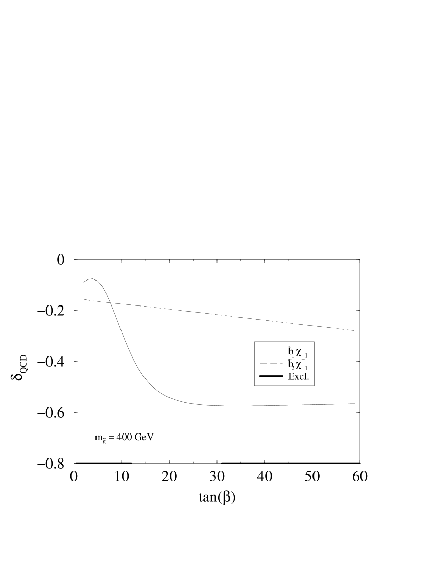
(a) (b)

Figure 6.5: The correction $\delta^{ai}_{QCD}$ to the decay width $\tilde{b}_{a}\rightarrow t\,\chi^{-}$ as a function of (a) $\tan\beta$  and (b) the higgsino mass parameter $\mu$. Set of inputs as in Fig. 6.2.

In Figs. 6.5-6.7 we present the evolution of the corrections (6.18) with some of the parameters. For the numerical evaluation we use $\alpha_{s}(m_{\tilde{b}_{a}})$, using the one-loop MSSM $\beta$-function, but, for the $m_{\tilde{b}_{a}}$ we use, it is basically the 4-flavour SM $\beta$-function, as the scale is almost always below the threshold of coloured SUSY  particles (and top quark). In Fig. 6.5 we can see the evolution with $\tan\beta$  and $\mu$, which are the most interesting ones. The corrections are large ($>10\%$) and present a weak evolution for large values of $\tan\beta$ ($\mbox{ \raisebox{-4.0pt}{${\stackrel{{\scriptstyle\textstyle>}}{{\sim}}}$} }20$). We remark that for $\mu<-120\,\mbox{ GeV}$ and $\tan\beta>20$ the corrections can be very large near the phase space limit of the lightest sbottom decay. However, this effect has nothing to do with the phase space exhaustion, which is described by the kinematic function $\lambda(a,i,t)$ on the RHS of the tree-level expression (6.6), but rather with the presence of the dynamical factor in brackets on that equation which also goes to the denominator of $\delta$ in eq.(6.7). That factor is fixed by the structure of the interaction Lagrangian of the sbottom decay into charginos and top; and, for the parameters in Fig. 6.5, it turns out to vanish near (actually past) the phase space limit in the case of the lightest sbottom ($\tilde{b}_{1}$) decay. However, this is not so either for the heaviest sbottom ($\tilde{b}_{2}$) or for $\mu>120\,\mbox{ GeV}$ as it is patent in the same figure. The different evolution that present the corrections of the two sbottoms has more relation with the electroweak nature of the process than with the purely QCD  loops, it is due to the fact that, being $\theta_{\tilde{b}}$ and $\theta_{\tilde{t}}$ so small, the squarks are mostly chiral, namely

$$\tilde{b}_{1}\simeq\tilde{b}_{R}\,\,\,\,,\,\,\,\tilde{b}_{2}\simeq\tilde{b}_{L}\,\,\,\,,\,\,\,\tilde{t}_{1}\simeq\tilde{t}_{R}\,\,\,\,,\,\,\,\tilde{t}_{2}\simeq\tilde{t}_{L}\,\,\,,$$ (6.19)

so its very different couplings to charginos (• ‣ 2.5) provides a very different evolution of (6.7), even if $\Lambda_{L,R}$ were constant. In fact the sbottom mixing angle plays a crucial role in this corrections as seen in Fig. 6.6, however we also see that its value is highly constrained by the condition (2.23). Finally we would like to comment on the effect of the gaugino mass parameter $M$ and the gluino mass in Fig. 6.7. The gluino evolution is rather flat once the pseudo-thresholds of $\tilde{b}_{a}\rightarrow b\,\tilde{g}$ are passed, so even though the gluino could not be produced at the Tevatron it would have an effect on the sbottom decay. As for the gaugino mass parameter the correction is saturated for $M\mbox{ \raisebox{-4.0pt}{${\stackrel{{\scriptstyle\textstyle>}}{{\sim}}}$} }200\mbox{ GeV}$, so the corrections computed in this section can be compared with the ones obtained in the higgsino approximation discussed in the next section.

The other parameters of the model present a rather mild effect on the corrections for squark masses in the ballpark of several hundreds of GeV. In summary the QCD  corrections on the decay $\tilde{b}_{a}\rightarrow t\,\chi^{-}_{i}$ are large ($\simeq-20\%$ for $\tilde{b}_{2}$, $\simeq-60\%$ for $\tilde{b}_{1}$) and negative for values of the parameter space relevant to the Tevatron energies, with a higgsino-like chargino and moderate or large $\tan\beta$.

Figure 6.6: The correction $\delta^{ai}_{QCD}$ as a function of $\theta_{\tilde{b}}$. Inputs as in Fig. 6.2.

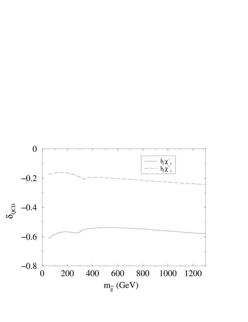
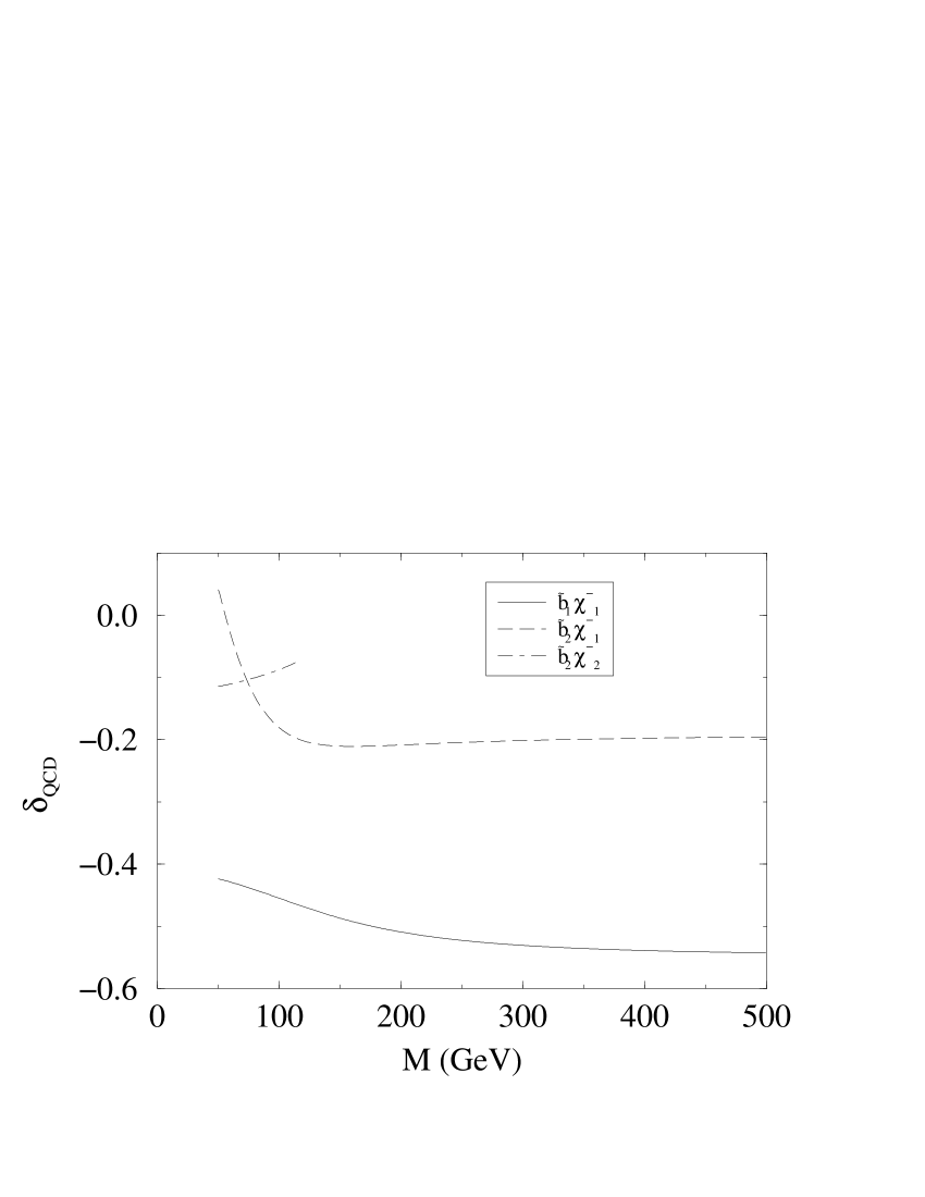
(a) (b)

Figure 6.7: The correction $\delta^{ai}_{QCD}$ as a function of (a) the gluino mass $m_{\tilde{g}}$  and (b) the gaugino mass parameter $M$. Set of inputs as in Fig. 6.2.

6.5 Yukawa corrections

At large ($\geq 20$) or small ($<1$) $\tan\beta$ these effects could be competitive with the QCD  corrections of the previous section. Since in these conditions the full MSSM quantum effects can be rather large, their calculation is indispensable to account for the observed top quark production cross-section (1.4) in the MSSM or, alternatively, to better assess how much the determination of the SM branching ratio $BR(t\rightarrow W^{+}\,b)$ is affected in the MSSM  context after plugging in the experimental number on the LHS of eq.(1.4).

The analytical formulation developed so far in chapter 3 and in section 6.2 is well suited to tackle the general problem of the SUSY-EW corrections to squark decays. Since the dominant part is from the Yukawa sector we wish to pursue our calculation in the following within the Yukawa coupling approximation. This means that we are going to compute the leading electroweak effects of ${\cal O}(\lambda^{2}_{t})$ and ${\cal O}(\lambda^{2}_{b})$ that emerge for large values of the Yukawa couplings (1.2) when the remaining gauge contributions – of ${\cal O}(g^{2})$– are subdominant. In practice we shall only explore the large $\tan\beta$ regime, typically $\tan\beta\geq 20$; the possibility $\tan\beta<1$ is not so appealing from the theoretical point of view. Thus within our approximation we will include the correction $\Delta_{\tau}$ in leading order ${\cal O}(\lambda_{\tau}^{2})$ of the $\tau$ Yukawa-coupling, $\lambda_{\tau}$. Notice furthermore that for $\lambda_{b}\gg 1$ the tree-level decay rate, eq. (6.6), is maximized. Therefore, the large $\tan\beta$ range is expected to be the most relevant one for the decay under consideration.

In our approach, we set the $SU(2)_{L}$ gaugino mass parameter $M\gg|\mu|,M_{W}$ in the chargino mass matrix (see section 2.4.4), and therefore the chargino $\chi^{\pm}_{1}$ is mainly higgsino, whereas the chargino $\chi^{\pm}_{2}$ is mainly gaugino and does not contribute to our decays. It is only in this case that the Yukawa-coupling approximation makes sense. Thus, since $m_{\tilde{t}_{1}}>80-90\,\mbox{ GeV}$, in this approach the decay into stop and neutralino $t\rightarrow\tilde{t}_{a}\,\chi^{0}_{\alpha}$ is kinematically forbidden. In this approximation the relevant counterterms $\delta A_{\pm ai}^{(b)}$ in eq.(6.2) boil down to

$$\delta A_{+a1}^{(b)} = -\delta R_{2a}^{(b)}\,\lambda_{b}-R_{2a}^{(b)}\,\delta\lambda_{b}$$

$$\delta A_{-a1}^{(b)} = -\delta R_{1a}^{(b)}\,\lambda_{t}-R_{1a}^{(b)}\,\delta\lambda_{t}\,.$$ (6.20)

(0,10)(0,10)(140,70) thin i1 o1 fermion,label=$\chi^{-}_{1}$,label.side=leftv1,o1 fermion,label=$\chi^{-}_{1}$,label.side=lefti1,v2 scalar,label=$\tilde{b}_{a}$,right,label.side=right,tension=0.5v2,v1 fermion,label=$t$,right,label.side=right,tension=0.5v1,v2	(0,10)(0,10)(140,70) thin i1 o1 fermion,label=$\chi^{-}_{1}$,label.side=leftv1,o1 fermion,label=$\chi^{-}_{1}$,label.side=lefti1,v2 fermion,label=$b$,right,label.side=right,tension=0.5v2,v1 scalar,label=$\tilde{t}_{a}$,right,label.side=right,tension=0.5v1,v2
(a)	(b)

Figure 6.8: Feynman graphs contributing to the chargino self-energy in the Yukawa approximation.

In the higgsino approximation only two Feynman graphs contribute to the $\chi^{-}_{1}$ self-energy, and they are depicted in Fig. 6.8. We can write the chargino $\chi^{-}_{1}$ self-energies, defined like the fermion self-energies in chapter 3, as

$$\Sigma_{L}^{1}(k^{2}) = -i\,g^{2}\,N_{C}(A_{-a1}^{(b)})^{2}B_{1}(k,m_{t},m_{\tilde{b}_{a}})$$

$$\Sigma_{R}^{1}(k^{2}) = -i\,g^{2}\,N_{C}(A_{+a1}^{(b)})^{2}B_{1}(k,m_{t},m_{\tilde{b}_{a}})$$

$$\Sigma_{S}^{1}(k^{2}) = +i\,g^{2}\,N_{C}\frac{m_{t}}{M_{i}}\epsilon_{i}\,A_{+a1}^{(b)}\,A_{-a1}^{(b)}\,B_{0}(k,m_{t},m_{\tilde{b}_{a}})\,\,,$$ (6.21)

for diagram 6.8(a), note that in this approximation the chargino $\chi^{-}_{1}$ coupling matrices are simply

(0,10)(0,10)(140,70) thin i1 o1 scalar,label=$\tilde{b}_{a}$,label.side=lefti1,v1 fermion,label=$t$,right,tension=0.5v1,v2 fermion,label=$\chi^{+}_{i}$,right,tension=0.5v2,v1 scalar,label=$\tilde{b}_{b}$,label.side=leftv2,o1	(0,10)(0,10)(140,70) thin i1 o1 scalar,label=$\tilde{b}_{a}$,label.side=lefti1,v1 fermion,label=$b$,right,tension=0.5v1,v2 fermion,label=$\chi^{0}_{\alpha}$,right,tension=0.5v2,v1 scalar,label=$\tilde{b}_{b}$,label.side=leftv2,o1
(a)	(b)
(0,10)(0,10)(140,70) thin i1 o1 scalar,label=$\tilde{b}_{a}$,label.side=lefti1,v1 scalar,label=$\tilde{t}_{c}$,right,tension=0.5v1,v2 scalar,label=$H^{+}\,,\,G^{+}$,right,tension=0.5v2,v1 scalar,label=$\tilde{b}_{b}$,label.side=leftv2,o1	(0,10)(0,10)(140,70) thin i1 o1 scalar,label=$\tilde{b}_{a}$,label.side=lefti1,v1 scalar,label=$\tilde{b}_{c}$,right,tension=0.5v1,v2 scalar,label=$h^{0}\,,\,H^{0}\,,\,A^{0}\,,\,G^{0}$,right,tension=0.5v2,v1 scalar,label=$\tilde{b}_{b}$,label.side=leftv2,o1
(c)	(d)
(0,30)(0,-30)(140,70) thin i1 o1 scalar,label=$\tilde{b}_{b}$,label.side=leftv1,o1 scalar,label=$\tilde{b}_{a}$,label.side=lefti1,v1 scalar,label=$h^{0}\,,\,H^{0}\,,\,A^{0}\,,\,G^{0}\,,\,H^{+}\,,\,G^{+}$,right,label.side=rightv1,v1
(e)

Figure 6.9: Feynman graphs contributing to the sbottom self-energy from the Electroweak sector.

$$A_{-a1}^{(b)}=-\lambda_{b}\,R_{2a}^{(b)}\,\,,\,\,A_{+a1}^{(b)}=-\lambda_{t}\,R_{1a}^{(b)}\,\,,$$

we prefer however to maintain a more general notation. The bottom-stop contribution (diagram 6.8(b)) can be obtained performing the following substitutions to (6.5): $m_{t}\rightarrow m_{b}$, $m_{\tilde{b}_{a}}\rightarrow m_{\tilde{t}_{a}}$, $A_{\pm ai}^{(b)}\rightarrow A_{\mp ai}^{(t)}$. From these self-energies we compute the wave function renormalization constants with the help of expression (3.11). A brief comment is mandatory respecting the relation between the renormalization constants (6.5) and that of the charged Higgs (3.55). The chargino definition (2.4.4), in the case of the higgsino approximation, is

$$\Psi_{1}^{-}=\left(\begin{array}[]{c}\tilde{H}_{1}^{-}\\ \bar{\tilde{H}}_{2}^{+}\end{array}\right)\,\,,$$ (6.22)

thus in a supersymmetric renormalization we should obtain that the wave function renormalization constants obtained from (6.5) are

$$\delta Z_{L}^{1}=\delta Z_{H_{1}}\,\,\,,\,\,\,\delta Z_{R}^{1}=\delta Z_{H_{2}}\,\,,$$ (6.23)

as we are not dealing with a supersymmetric renormalization procedure this is not the case, however we have checked that the divergent part of this different renormalization constants is the same. This fact is crucial in the cancellation of the divergences of $\delta Z_{\{L,R\}}^{1}$ with the term $\delta Z_{H^{\pm}}$ appearing in the definition of $\delta\tan\beta$ (3.51).

From diagrams of figure 6.9 we can obtain the sbottom self-energies. The chargino top contribution from Fig. 6.9(a) is

$$\Sigma_{ab}^{\chi^{-}}(k^{2}) = -i\,2\,g^{2}\left[\left(A_{+bi}^{(b)}\,A_{+ai}^{(b)}+A_{-bi}^{(b)}\,A_{-bi}^{(b)}\right)(\tilde{B}_{0}+k^{2}\,B_{1})\right.$$ (6.24)

$$\left.+\epsilon_{i}\,M_{i}\,m_{t}(A_{+bi}^{(b)}\,A_{-ai}^{(b)}+A_{-bi}^{(b)}\,A_{+ai}^{(b)})B_{0}\right](k,M_{i},m_{t})\,\,,$$

and the Higgs contributions from diagrams 6.9(c) and (d) is simply

$$\Sigma_{ab}^{H}(k^{2})=i\,g^{2}\sum_{c}R_{ia}^{(b)}\,R_{jc}^{(q)*}\,G^{H}_{ij}\,R_{kc}^{(q)}\,R_{lb}^{(b)*}\,G^{H}_{lk}B_{0}(k,m_{\tilde{q}_{c}},M_{H})\,\,,$$ (6.25)

with $H=(H^{+},G^{+};h^{0},H^{0},A^{0},G^{0})$, $\tilde{q}=(\tilde{t};\tilde{b})$, and $G^{H}_{ij}$ is the Feynman rule for $H\rightarrow\tilde{q}_{i}^{*}\,\tilde{q}_{j}^{\prime}$, with $\tilde{q}_{1,2}$ the weak eigenstates squarks, divided by $-ig$ [39, 71]. On the other hand diagram 6.9(e) only contributes to the mass counterterm and mixing wave function renormalization constants,

$$\Sigma_{ab}^{HH}=i\,g^{2}\sum_{H^{+},G^{+}}R_{ia}^{(b)}\,R^{(b)*}_{jb}\,E^{H}_{ij}A_{0}(M_{H})+\frac{i\,g^{2}}{2}\sum_{h^{0},H^{0},A^{0},G^{0}}R_{ia}^{(b)}\,R^{(b)*}_{jb}\,E^{H}_{ij}A_{0}(M_{H})\,\,,$$ (6.26)

with $E^{H}_{ij}$ the corresponding Feynman rule of $H\,H^{*}\rightarrow\tilde{b}^{\prime*}_{i}\,\tilde{b}^{\prime}_{j}$, $\tilde{b}_{1,2}$ the weak eigenstate squarks, divided by $-ig^{2}$[39].

Then the diagonal wave function renormalization constant is

$$\delta Z_{aa}^{\chi^{-}} = -i\,2\,g^{2}\left[\frac{1}{2}\left((A_{+ai}^{(b)})^{2}+(A_{-ai}^{(b)})^{2}\right)\left((m_{t}^{2}+3\,M^{2}_{i}+m_{\tilde{b}_{a}}^{2})B_{0}^{\prime}-B_{0}\right)\right.$$ (6.27)

$$+ \left.2\,\epsilon_{i}\,M_{i}\,m_{t}\,A_{+ai}^{(b)}\,A_{-ai}^{(b)}\,B_{0}^{\prime}\right](m_{\tilde{b}_{a}},M_{i},m_{t})\,\,,$$

$$\delta Z_{aa}^{H} = i\,g^{2}\sum_{c}R_{ia}^{(b)}\,R_{jc}^{(q)*}\,G^{H}_{ij}\,R_{kc}^{(q)}\,R_{lb}^{(b)*}\,G^{H}_{lk}B_{0}^{\prime}(m_{\tilde{b}_{a}},m_{\tilde{q}_{c}},M_{H})\,\,.$$ (6.28)

The neutralino-bottom contribution form Fig. 6.9(b) can be easily found by performing the following transformations in expressions (6.24) and (6.27): substitute $m_{t}\rightarrow m_{b}$, the chargino indices by neutralino ones $i\rightarrow\alpha$, and divide the expressions by $2$.

The rest of the renormalization constants are computed using the very same expressions of chapter 3 by taking the Yukawa approximation, i.e.  by removing the interactions with the gauge bosons (but maintaining that of the Goldstone bosons) and with the gauginos.

(0,15)(0,5)(200,80) thin i1 o2,o1 scalar,label.side=left,label=$\tilde{b}_{a}$i1,v1 fermion,label.side=left,label=             $t$v2,o1 fermion,label.side=right,label=             $\chi^{-}_{i}$o2,v3 scalar,label=$h^{0}\,,\,H^{0}\,,\,A^{0}\,,\,G^{0}$v1,v2 fermion,label=$t$,label.side=rightv3,v2 scalar,label=$\tilde{b}_{b}$,label.side=rightv1,v3 .6w,1hv2 .6w,0v3 .3w,.5hv1	(0,15)(0,5)(200,80) thin i1 o2,o1 scalar,label.side=left,label=$\tilde{b}_{a}$i1,v1 fermion,label.side=left,label=             $t$v2,o1 fermion,label.side=right,label=             $\chi^{-}_{i}$o2,v3 fermion,label=$\chi^{0}_{\alpha}$v1,v2 scalar,label=$\tilde{t}_{b}$,label.side=rightv3,v2 fermion,label=$b$,label.side=rightv1,v3 .6w,1hv2 .6w,0v3 .3w,.5hv1
(a)	(b)

Figure 6.10: Feynman diagrams contributing to the one-loop vertex form factors of the decay $\tilde{b}_{a}\rightarrow t\,\chi^{-}_{i}$ in the Yukawa approximation.

The one-loop Feynman diagrams contributing to the vertex form factors can be seen in Fig. 6.10. There exists other possible diagrams, but they do not contribute in the Yukawa approximation. From this diagrams we can compute the corresponding $F_{\{L,R\}}$ form factors,

$$F_{L}^{\{h^{0},H^{0}\}} = N_{\{h^{0},H^{0}\}}\left[m_{t}\,\epsilon_{i}\,A_{-bi}^{(b)}(C_{12}-C_{11})-M_{i}\,A_{+bi}^{(b)}C_{12}+m_{t}\,\epsilon_{i}\,A_{-bi}^{(b)}\,C_{0}\right]\,\,,$$

$$F_{R}^{\{h^{0},H^{0}\}} = N_{\{h^{0},H^{0}\}}\left[m_{t}\,A_{+bi}^{(b)}(C_{12}-C_{11})-M_{i}\,\epsilon_{i}\,A_{-bi}^{(b)}C_{12}+m_{t}\,A_{+bi}^{(b)}\,C_{0}\right]\,\,,$$

$$N_{\{h^{0},H^{0}\}} = -i\,g^{2}\frac{\lambda_{t}}{2}\{\sin\alpha,\cos\alpha\}G^{\{h^{0},H^{0}\}}_{ij}R^{(b)}_{ia}R^{(b)*}_{jb}\,\,,$$

$$F_{L}^{\{A^{0},G^{0}\}} = N_{\{A^{0},G^{0}\}}\left[-m_{t}\,\epsilon_{i}\,A_{-bi}^{(b)}(C_{12}-C_{11})-M_{i}\,A_{+bi}^{(b)}\,C_{12}+m_{t}\,\epsilon_{i}\,A_{-bi}^{(b)}\,C_{0}\right]\,\,,$$

$$F_{R}^{\{A^{0},G^{0}\}} = N_{\{A^{0},G^{0}\}}\left[m_{t}\,A_{+bi}^{(b)}\,(C_{12}-C_{11})+M_{i}\,\epsilon_{i}A_{-bi}^{(b)}\,C_{12}-m_{t}\,A_{+bi}^{(b)}\,C_{0}\right]\,\,,$$

$$N_{\{A^{0},G^{0}\}} = -i\frac{g^{2}}{2\,\sqrt{2}\,M_{W}}\{-\frac{m_{t}\,\cot\beta}{\sqrt{2}},-m_{t}\}G^{\{A^{0},G^{0}\}}_{ij}R^{(b)}_{ia}R^{(b)*}_{jb}\,\,,$$

$$C_{*} = C_{*}(-p,k,m_{t},m_{\Phi^{0}},m_{\tilde{b}_{b}})\,\,,$$ (6.29)

for diagram 6.10(a), and with the help of the following combinations

$$\begin{array}[]{rclrcl}A^{(1)}&=&A_{+b\alpha}^{(t)}\,A_{-bi}^{(t)}\,A_{-a\alpha}^{(b)}\,,&A^{(5)}&=&\epsilon_{\alpha}\,A_{-b\alpha}^{(t)}\,A_{-bi}^{(t)}\,A_{-a\alpha}^{(b)}\,,\\ A^{(2)}&=&A_{+b\alpha}^{(t)}\,A_{-bi}^{(t)}\,\epsilon_{\alpha}\,A_{+a\alpha}^{(b)}\,,&A^{(6)}&=&A_{-b\alpha}^{(t)}\,A_{-bi}^{(t)}\,A_{+a\alpha}^{(b)}\,,\\ A^{(3)}&=&A_{+b\alpha}^{(t)}\,\epsilon_{i}A_{+bi}^{(t)}\,A_{-a\alpha}^{(b)}\,,&A^{(7)}&=&\epsilon_{\alpha}\,A_{-b\alpha}^{(t)}\,\epsilon_{i}\,A_{+bi}^{(t)}\,A_{-a\alpha}^{(b)}\,,\\ A^{(4)}&=&A_{+b\alpha}^{(t)}\,A_{+bi}^{(t)}\,\epsilon_{\alpha}\,A_{+a\alpha}^{(b)}\,,&A^{(8)}&=&A_{-b\alpha}^{(t)}\,\epsilon_{i}\,A_{+bi}^{(t)}\,A_{+a\alpha}^{(b)}\,,\\ \end{array}$$ (6.30)

the contribution from diagram diagram 6.10(b) is

$$F_{L}^{\chi} = -i\frac{g^{2}}{4}\left[C_{0}(M_{i}\,m_{t}\,A^{(3)}+m_{t}\,m_{b}\,A^{(4)}+M^{0}_{\alpha}\,M_{i}\,A^{(5)}+M^{0}_{\alpha}\,m_{b}\,A^{(8)})\right.$$

$$- m_{t}\,(C_{11}-C_{12})(M_{i}\,A^{(3)}+m_{b}\,A^{(4)}+m_{t}\,A^{(6)}+M^{0}_{\alpha}\,A^{(2)})$$

$$+ \left.M_{i}\,C_{12}(M_{i}\,A^{(6)}+m_{b}\,A^{(5)}+m_{t}\,A^{(6)}+M^{0}_{\alpha}\,A^{(7)})+\tilde{C}_{0}\right]\,\,,$$

$$F_{R}^{\chi} = F_{L}^{\chi}\left\{A^{(i)}\leftrightarrow A^{(9-i)}\right\}\,\,,$$

$$C_{*} = C_{*}(-p,k,m_{\tilde{t}_{b}},M^{0}_{\alpha},m_{b})\,\,.$$ (6.31)

For the numerical analysis, we follow the directions given in section 6.3. In the relevant large $\tan\beta$ segment under consideration, namely

$$20\mbox{ \raisebox{-4.0pt}{${\stackrel{{\scriptstyle\textstyle<}}{{\sim}}}$} }\tan\beta\mbox{ \raisebox{-4.0pt}{${\stackrel{{\scriptstyle\textstyle<}}{{\sim}}}$} }40\,,$$ (6.32)

the bottom quark Yukawa coupling $\lambda_{b}$ is comparable to the top quark Yukawa coupling, $\lambda_{t}$. Even though the extreme interval $40<\tan\beta<60$ can be tolerated by perturbation theory, we shall confine ourselves to the moderate range (6.32). This is necessary to preserve the condition (2.23) for the typical set of sparticle masses used in our analysis. We point out that the colour stability requirement (2.23) could be satisfied independently of $\tan\beta$ if the $A$-parameters would be chosen directly as a part of the set of inputs and then taken sufficiently small. Nevertheless this possibility is not so convenient in our analysis where the sparticle masses are the natural inputs that we wish to control in order to make sure that sparticles can be produced and decay at the Tevatron as explained in connection to eq.(1.4).

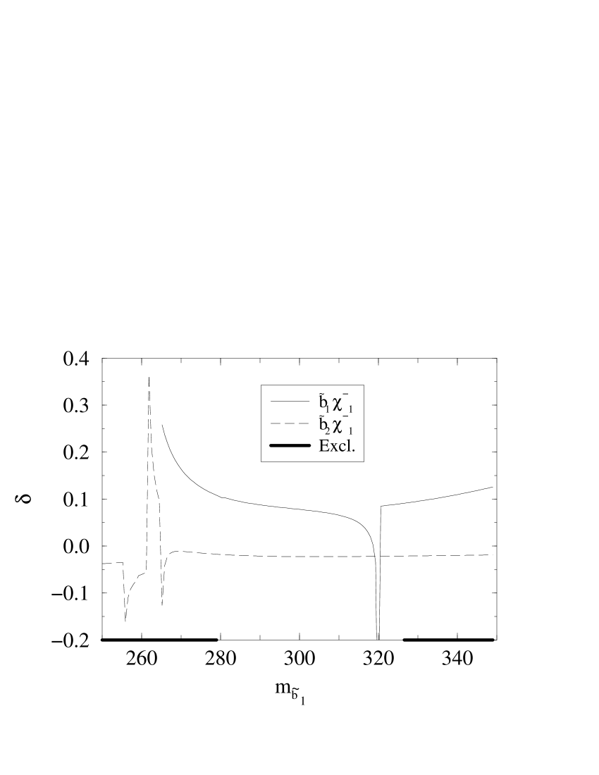
(a)	(b)

Figure 6.11: (a) The SUSY-EW corrections (6.7) as a function of $m_{\tilde{t}_{1}}$; (b) As in (a), but as a function of $m_{\tilde{b}_{1}}$. Rest of inputs as in Fig. 6.2.

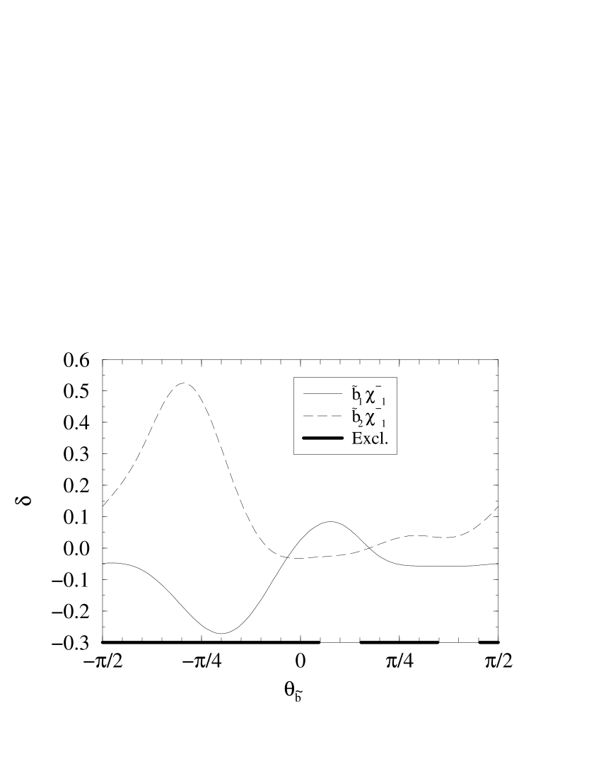
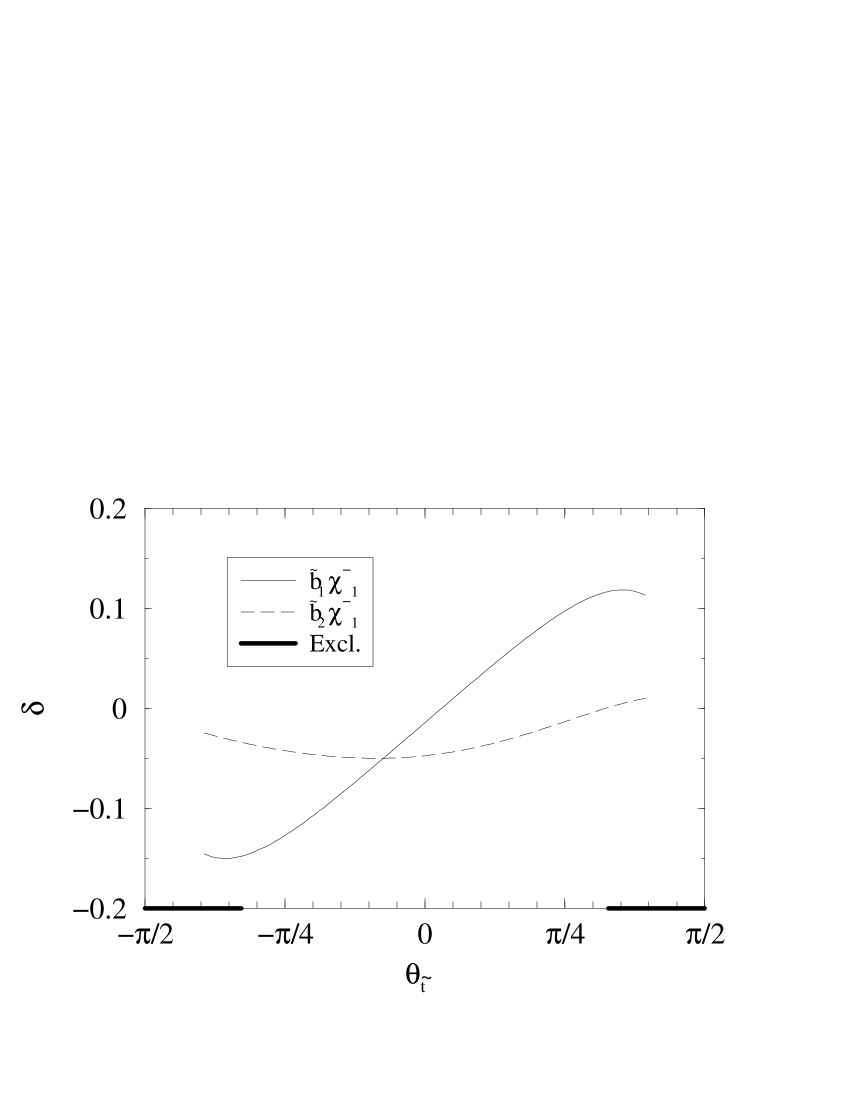
(a)	(b)

Figure 6.12: (a) Evolution of the SUSY-EW corrections as a function of the sbottom mixing angle, ${\theta}_{\tilde{b}}$, within its allowed range; (b) As in (a), but as a function of the stop mixing angle, ${\theta}_{\tilde{t}}$. Remaining inputs are as in Fig. 6.2.

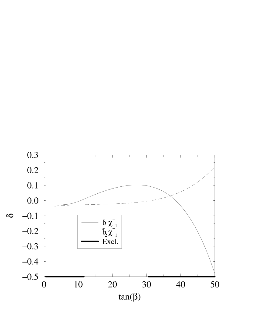
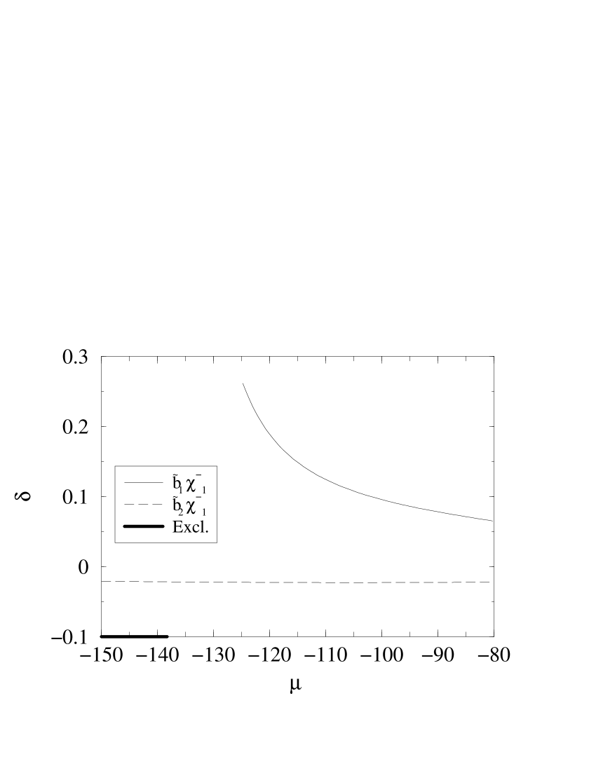
(a)	(b)

Figure 6.13: (a) The SUSY-EW correction as a function of $\tan\beta$; (b) As in (a), but as a function of $\mu$. Rest of inputs and notation as in Fig. 6.2.

The corresponding corrections $\delta^{ai}$ (6.7) are shown in Figs. 6.11(a) and 6.11(b) as a function of the lightest stop and sbottom masses, respectively. The allowed range for the sbottom and stop mixing angles is conditioned by the upper bound on the trilinear couplings and is obtained from eqs.(6.10) and (2.23). In the physical $\theta_{\tilde{b}}$ range, the variation of the correction (6.7) is shown in Fig. 6.12(a). On the other hand the permitted range for the stop mixing angle, $\theta_{\tilde{t}}$, is much larger and we have plotted the corrections within the allowed region in Fig. 6.12(b). Notice that the sign of the quantum effects changes within the domain of variation of $\theta_{\tilde{t}}$. Finally, we display the evolution of the SUSY-EW effects as a function of $\tan\beta$ (Fig. 6.13(a)) and of $\mu$ (Fig. 6.13(b)) within the region of compatibility with the constraint (2.23).

A few more words are in order to explain the origin of the leading electroweak effects. One could expect that they come from the well-known large $\tan\beta$ enhancement stemming from the chargino-stop corrections to the bottom mass (Cf. Fig. 4.4(b)). Nonetheless this is only partially true, for in the present case the remaining contributions (Cf. Figs. 6.8, 6.9 and 6.10) can be sizeable enough. One can also think on the SUSY  counterpart of Fig. 4.4(b), which we have depicted in Fig. 6.14, as an additional leading contribution, as, in addition to the $\tan\beta$  enhancement, has an $A_{q}$ enhancement. However the addition of these two kind of contributions does not account for the total behaviour in all of the parameter space. To be more precise, in the region of the parameter space that we have dwelled upon the bottom mass contribution is seen to be dominant only for the lightest sbottom decay and for the lowest values of $\tan\beta$ in the range (6.32). This is indeed the case in Fig. 6.12(b) where $\tan\beta=20$ and therefore the bottom mass effect modulates the electroweak correction in this process and $\delta^{11}$ becomes essentially an odd function of the stop mixing angle. This fact is easily understood since, as noted above, sbottoms are mostly chiral –eq. (6.19)– and the $\tilde{b}_{R}$ is the only one with couples with $\lambda_{b}$ –eq. (2.5). On the other hand, from Fig. 6.13(a) it is obvious that the (approximate) linear behaviour on $\tan\beta$ expected from bottom mass renormalization becomes completely distorted by the rest of the contributions, especially in the high $\tan\beta$ end. In short, the final electroweak correction cannot be simply ascribed to a single renormalization source but to the full Yukawa-coupling combined yield.

In general the SUSY-EW  corrections to $\Gamma(\tilde{b}_{a}\rightarrow t\,\chi^{-}_{i})$ are smaller than the QCD  corrections. The reason why the electroweak corrections are smaller is in part due to the condition (2.23) restricting our analysis within the $\tan\beta$ interval (6.32). From Figs. 6.12 and 6.13(a) it is clear that outside this interval the SUSY-EW  contributions could be much higher and with the same or opposite sign as the QCD  effects, depending on the choice of the sign of the mixing angles. Moreover, since we have focused our analysis to sbottom masses accessible to Tevatron, again the theoretical bound (2.23) severely restricts the maximum value of the trilinear couplings and this prevents the electroweak corrections from being larger. This cannot be cured by assuming larger values of $M_{H}$ and/or of $\mu$ due to our assumption that $t\rightarrow H^{+}\,b$ is operative and because $\mu$ directly controls the value of the (higgsino-like) chargino final state in our decay, so that basically we have $|\mu|<m_{\tilde{b}_{a}}-M_{H}$. The restriction cannot be circumvented either if we assume larger values of $m_{\tilde{t}_{a}}$, for it has been shown that too heavy stops are incompatible with the CLEO data on $b\rightarrow s\,\gamma$ both at low and high $\tan\beta$ [60, 148, 164, 165, 166, 167, 168, 169, 170]. We point out that the MSSM  analysis of $b\rightarrow s\,\gamma$ also motivated the sign choice $A\,\mu<0$ in our numerical calculation [60]. Admittedly, the situation with radiative $B$-decays is still under study and there are many sources of uncertainties that deserve further experimental consideration. Still, we have used this information to focus on a limited domain of the MSSM  parameter space.

(0,10)(0,0)(180,90) thin i1 o1 scalar,label=$\tilde{b}_{L}$,label.side=lefti1,v1 scalar,label=$H^{+}\,,\,\ G^{+}$,left,tension=0.5v2,v1 dashes,label=,left,tension=0.5v1,v2 scalar,label=$\tilde{b}_{R}$,label.side=leftv2,o1 phantom,label=$\tilde{t}_{R}$,label.side=left,label.dist=.3cm,tension=0v1,v3 phantom,label=$\tilde{t}_{L}$,label.side=left,label.dist=.3cm,tension=0v3,v2 label=$m_{t}M_{LR}^{t}$,label.dist=.3cm,label.angle=90,decor.shape=crossv3 .5w,.84hv3

Figure 6.14: Finite Feynman diagram contributing to the $\tilde{b}$  mixed self-energy in the EW  basis.

6.6 Conclusions

In summary, the MSSM  corrections to squark decays into charginos and neutralinos can be significant and therefore must be included in any reliable analysis of top quark physics at the Tevatron within the MSSM. The main corrections stem from the strongly interacting sector of the theory (i.e. the one involving gluons and gluinos), but also non-negligible effects may appear from the electroweak sector (characterized by chargino-neutralino exchange) at large (or very small) values of $\tan\beta$. Failure of including these corrections in future studies of top quark physics at the Tevatron, both in the production and decay mechanisms, might seriously hamper the possibility of discovering clear-cut traces of SUSY  physics from the identification of large non-SM quantum corrections in these processes. As already stated, we have mainly concentrated on the impact of these quantum signatures in the physics of the Tevatron, but important effects are also expected for experiments aiming at the production and decay of “obese” squarks at the LHC. The latter type of squarks could be free of some of the restrictions that have been considered for the present calculation.

The present study has also an impact on the determination of squark parameters at the LC. The squark masses used in it are available already for a LC running at a center of mass energy of $800\mbox{ GeV}$. The large corrections of both, the QCD  and the EW  sector (in the Yukawa approximation), makes them necessary, not only for prospects of precision measurements in the sbottom-chargino-neutralino sectors, but also for a reliable first determination of its parameters.

Chapter 7 Conclusions

In this Thesis we have performed a study of some of the possible phenomenological consequences deriving from the interactions between the third generation matter supermultiplet and the the super-Higgs boson sector of the MSSM  at the one-level, with especial emphasis on the implications for the top quark and Higgs-boson physic at the Tevatron collider. We have done so in the on-shell renormalization scheme, using a physically motivated definition of $\tan\beta$. Our definition of $\tan\beta$  has the virtue of automatically incorporating the one-loop radiative corrections to the most plausible signature of the charged Higgs (if $\tan\beta>2$), namely the $\tau\,\nu_{\tau}$ channel. Remarkably enough, this definition of $\tan\beta$  can also be extended to the situation when $M_{H^{\pm}}>m_{t}$ for a wide range of heavy charged Higgs masses to be explored at the LHC rather than at the Tevatron [60, 61]. For it turns out that the branching ratio of the charged Higgs into $\tau$ never becomes negligible in that range.

• The effects of one-loop EW  radiative corrections to the unconventional top quark decay mode $t\rightarrow H^{+}b$ are large in the moderate and specially in the high regime of $\tan\beta$, where they can easily reach values of

  $$\delta_{EW}(t\rightarrow H^{+}\,b)\simeq+30\%$$ (7.1)

  for negative $\mu$ (and positive $A_{t}$) and a “light” sparticle spectrum (Fig. 4.6), and

  $$\delta_{EW}(t\rightarrow H^{+}\,b)\simeq+20\%$$ (7.2)

  for positive $\mu$ (and negative $A_{t}$) and heavy sparticle spectrum (Fig. 4.19). In both cases we have singled out the domain $\mu A_{t}<0$ of the parameter space, which is the one preferred by the experimental data on radiative B-meson decays ($b\rightarrow s\gamma$).

  The previous results should be compared with the QCD and SUSY-QCD  corrections which in previous studies [42, 48] were shown to reach values of $\delta_{QCD}\simeq-60\%$, $\delta_{SUSY-QCD}\simeq+80\%$ and $\delta_{SUSY-QCD}\simeq-40\%$ for the same scenarios. In the perturbative regime of the calculation, the positive EW  corrections attained for $\mu>0$ ($\mu A_{t}<0$) can be of the same order as they are in the $\mu<0$ ($\mu A_{t}<0$) case. Unfortunately, the EW  effects never become huge enough so as to prevent the total MSSM  correction from being highly negative for $\mu>0$ ($\mu A_{t}<0$) – an unlucky fact which unavoidably leads to a severe suppression of the corresponding branching ratio in this case. Quite in contrast, in the $\mu<0$ ($\mu A_{t}<0$) situation there are indeed regions of the parameter space where the positive EW  corrections could be perfectly visible; namely, in those places where the total QCD  correction in the MSSM  largely cancels out, e.g. around $\tan\beta=30$ in Fig. 4.6(a). Negative corrections of the same order can be obtained provided $\mu A_{t}>0$ (Cf. Fig 4.10(b)).

  From these considerations it follows that, if there exists supersymmetric partners of the standard particles at a scale $100-500\mbox{ GeV}$, the unconventional top quark decay mode $t\rightarrow H^{+}\,b$ has a partial width that differs significantly from the conventional QCD expectations. In this case the analyses of the Tevatron data could exclude a region in the $\tan\beta-M_{H^{\pm}}$ plane which is substantially modified as compared to recent analyses from the Tevatron collaborations. Thus e.g. for a charged Higgs mass of $110\mbox{ GeV}$, and using the conventional QCD  corrected value for the decay width $\Gamma(t\rightarrow H^{+}\,b)$, present Tevatron data implies that the excluded region is

  $$\tan\beta\geq 50\,\,.$$ (7.3)

  If, instead, we assume that the charged Higgs belongs to the Higgs sector of the MSSM, then we find that the excluded values of $\tan\beta$  are

  $$\tan\beta\geq 35\,\,,\,\,\tan\beta\geq 75\,\,,$$ (7.4)

  for the two scenarios presented above respectively (see Figs 4.23 and 4.24). Remarkably there is a range in the parameter space (characterized by $\mu>0$, $\mu A_{t}<0$) where no value of the $\tan\beta-M_{H^{\pm}}$ plane is excluded at all by present data on the charged Higgs decay of the top quark. Although in mSUGRA models in the literature one usually claims $A_{t}<0$, we already emphasized in chapter 4 that this is not necessary the case, especially at large $\tan\beta$  and for sufficiently large values of the trilinear Soft-SUSY-breaking parameter, $A_{0}$, at the unification scale. Thus, also in specific minimal SUGRA models, one can have $A_{t}>0$ and so $\mu<0$, which is the most attractive possibility since one achieves large positive corrections to $t\rightarrow H^{+}\,b$ compatible with $BR(b\rightarrow s\gamma)$.

  The bulk of the EW  corrections is given by the finite corrections to the bottom quark mass (or the bottom Yukawa coupling), which are proportional to $-\mu A_{t}$ -see eq. (4.31). However, it should be mentioned that there are cancellations among other sources of significant corrections. This fact implies that the rest of the SUSY  corrections was not obviously negligible from the very beginning. Thus, present CLEO data on the partial decay branching ratio $BR(b\rightarrow s\gamma)$[174] favours positive values of the EW  corrections. However, the leading component of the quantum effects is the SUSY-QCD  contribution which depends on the sign of $\mu$ (rather than that of $A_{t}\mu$). Therefore, in the end the sign that really matters for this process is that of $\mu$ alone. The best possible situation for the charged Higgs decay of the top quark would occur for negative $\mu$, since then the SUSY-QCD  corrections are positive, and the EW  corrections are also positive due to the $b\rightarrow s\,\gamma$ constraint. On the other hand, if $\mu$ is positive, then the total MSSM  correction is negative (in spite of the EW  component which must stay positive). In this case the bounds on the $(\tan\beta,M_{H^{\pm}})$ space could disappear, as we said above. And in these circumstances, as explained in chapter 4, there is an alternative scenario with relatively light neutral MSSM Higgs boson which in combination with the negative $t\rightarrow H^{+}\,b$ searches could strongly point towards the SUSY  nature of these Higgs bosons. As for the one-loop Higgs corrections sector of the MSSM, the over-all correction to the decay under consideration is very small due to huge cancellations triggered by the SUSY structure of the Higgs potential to this decay except for very low values of $\tan\beta$ (Fig. 4.6). Work is currently in progress to determine the effects of these large corrections to the top quark and charged Higgs associated production at the Tevatron and at the LHC.

• FCNC  top quark decays into neutral Higgs particles have been reviewed. The correct inclusion of the left-right mixing between squarks implies an enhancement of the partial branching ratio $BR(t\rightarrow ch)$ of two orders of magnitude with respect previous estimates. We have performed a separate analysis of the SUSY-EW  and SUSY-QCD  effects, with different approximations. For the SUSY-EW  sector we have used the super-CKM basis, whereby FCNC  are produced through the charged sector, as in the SM. For the SUSY-QCD  estimate we have supposed a non-flavour-diagonal mass elements in the left-chiral squark matrix. We have applied present bounds from EW precision data to these elements. The theoretical upper limits of these contributions to the decay width of the top quark are found to be (Figs. 5.5 and 5.8)

  $$BR^{\rm SUSY-EW}(t\rightarrow c\,h) {\stackrel{{\scriptstyle\textstyle<}}{{\sim}}} \mbox{ several }\times 10^{-6}$$

  $$BR^{\rm SUSY-QCD}(t\rightarrow c\,h) {\stackrel{{\scriptstyle\textstyle<}}{{\sim}}} \mbox{ several }\times 10^{-4}\,\,\,,$$ (7.5)

  and the typical values for this ratio are $10^{-8}$ and $10^{-5}-10^{-4}$ for the SUSY-EW and SUSY-QCD  induced FCNC  decays respectively. We have found that the SUSY-QCD  induced FCNC decay widths are at least two orders of magnitude larger than the SUSY-EW  ones in most of the parameter space, thus making unnecessary the computation of both the interference terms and FCNC EW  induced effects through non-flavour-diagonal mass terms. If data improves the bounds on these mass terms they will become more strict, bringing the SUSY-QCD  induced branching ratios down to the values of the SUSY-EW  ones, and then a complete computation would be needed, if there would be any hope at all to see these effects at the small branching ratio predicted by EW  corrections! The value found for $BR(t\rightarrow ch)$ is not sufficiently large to yield measurable effects at the Tevatron or at the LC. There is, however, a possibility that this decay mode could be measured at the LHC.

• If bottom-like squarks are heavy enough they could decay into a top quark and a chargino. This could serve as an unexpected source of top quarks at the Tevatron, at the LHC, or at the LC. The radiative corrections to the partial decay width $\tilde{b}\rightarrow t\,\chi^{-}$ are large, both the QCD  and the EW-like in the Yukawa approximation. In the case of the QCD  corrections, they are negative in most of the MSSM  parameter space accessible to Tevatron. These corrections are of the order

  $$\delta_{QCD}(\tilde{b}_{1}\rightarrow t\,\chi^{-}_{1}) \simeq -60\%$$

  $$\delta_{QCD}(\tilde{b}_{2}\rightarrow t\,\chi^{-}_{1}) \simeq -20\%$$ (7.6)

  for a wide range of the parameter space (Fig. 6.5). In certain corners of this space, though, they vary in a wide range of values. EW  corrections can be of both signs. Our renormalization prescription uses the mixing angle between squarks as an input parameter. This prescription forces the physical region to a narrow range when we require that colour breaking vacua is not generated. Within this restricted region the typical corrections vary in the range (Figs. 6.12, 6.13)

  $$\delta_{EW}(\tilde{b}_{1}\rightarrow t\,\chi^{-}_{1}) \simeq +25\%\mbox{ to }-15\%$$

  $$\delta_{EW}(\tilde{b}_{2}\rightarrow t\,\chi^{-}_{1}) \simeq +5\%\mbox{ to }-5\%\,\,,$$ (7.7)

  However we must recall that these limits are qualitative. In the edge of such regions we find the largest EW contributions. We stress that in this case it is not possible to narrow down the bulk of the corrections to just the renormalization of the bottom quark Yukawa coupling. Although it is true that for moderate values of the parameters (and for the lightest sbottom decay) the finite threshold corrections to the bottom Yukawa coupling yields most of the contribution, as soon as we take the parameters away of this central values the total corrections deviate significantly from the ones obtained using this only term. More work is presently in progress to generalize this results to the full SUSY-EW  sector, by incorporating the neutralino-like decays, and also the inclusion of gaugino-higgsino mixing.

Our general conclusion is that the supersymmetric strong and electroweak radiative corrections can be very important in the top/bottom-Higgs super-sector of the MSSM. Therefore, it is necessary to account for these corrections in the theoretical computation of the high energy physics observables, otherwise highly significant information on the potentially underlying SUSY  dynamics could be missed. This is true, not only for the future experiments at the LHC and the LC, but also for the present Run I data (and the Run II data around the corner) at the Fermilab Tevatron collider [221].

Appendix A Vertex functions

In this appendix we briefly collect, for notational convenience, the basic vertex functions frequently referred to in the text. The given formulas are exact for arbitrary internal masses and external on-shell momenta. Most of them are an adaptation to the $g_{\mu\nu}=\{+\,-\,-\,-\}$ metric of the standard formulae of Refs.[100, 101, 103]. The basic one-, two- and three-point scalar functions are:

$$A_{0}(m) = \int d^{n}\tilde{q}\,\frac{1}{[q^{2}-m^{2}]},$$ (A.1)

$$B_{0}(p,m_{1},m_{2}) = \int d^{n}\tilde{q}\,\frac{1}{[q^{2}-m_{1}^{2}]\,[(q+p)^{2}-m_{2}^{2}]}\,,$$ (A.2)

$$C_{0}(p,k,m_{1},m_{2},m_{3})=\int d^{n}\tilde{q}\,\frac{1}{[q^{2}-m_{1}^{2}]\,[(q+p)^{2}-m_{2}^{2}]\,[(q+p+k)^{2}-m_{3}^{2}]}\,;$$ (A.3)

using the integration measure

$$d^{n}\tilde{q}\equiv{\mu}^{(4-n)}\frac{d^{n}q}{(2\pi)^{n}}\,.$$ (A.4)

The two and three-point tensor functions needed for our calculation are the following

$$[\tilde{B}_{0},B_{\mu},B_{\mu\nu}](p,m_{1},m_{2})=\int d^{n}\tilde{q}\,\frac{[q^{2},q_{\mu},q_{\mu}q_{\nu}]}{[q^{2}-m_{1}^{2}]\,[(q+p)^{2}-m_{2}^{2}]}\,,$$ (A.5)

$$[\tilde{C}_{0},C_{\mu},C_{\mu\nu}](p,k,m_{1},m_{2},m_{3})=$$ (A.6)

$$\int d^{n}\tilde{q}\,\frac{[q^{2},q_{\mu},q_{\mu}q_{\nu}]}{[q^{2}-m_{1}^{2}]\,[(q+p)^{2}-m_{2}^{2}]\,[(q+p+k)^{2}-m_{3}^{2}]}\,.$$

By Lorentz covariance, they can be decomposed in terms of the above basic scalar functions and the external momenta:

$$\tilde{B}_{0}(p,m_{1},m_{2}) = A_{0}(m_{2})+m_{1}^{2}B_{0}(p,m_{1},m_{2})\,\,,$$

$$B_{\mu}(p,m_{1},m_{2}) = p_{\mu}B_{1}(p,m_{1},m_{2})\,\,,$$

$$B_{\mu\nu}(p,m_{1},m_{2}) = p_{\mu}p_{\nu}B_{21}(p,m_{1},m_{2})+g_{\mu\nu}B_{22}(p,m_{1},m_{2})\,\,,$$

$$\tilde{C}_{0}(p,k,m_{1},m_{2},m_{3}) = B_{0}(k,m_{2},m_{3})+m_{1}^{2}C_{0}(p,k,m_{1},m_{2},m_{3})\,\,,$$

$$C_{\mu}(p,k,m_{1},m_{2},m_{3}) = p_{\mu}C_{11}+k_{\mu}C_{12}\,\,,$$

$$C_{\mu\nu}(p,k,m_{1},m_{2},m_{3}) = p_{\mu}p_{\nu}C_{21}+k_{\mu}k_{\nu}C_{22}+(p_{\mu}k_{\nu}+k_{\mu}p_{\nu})C_{23}+g_{\mu\nu}C_{24}\,\,,$$ (A.7)

where we have defined the Lorentz invariant functions:

$$B_{1}(p,m_{1},m_{2}) = \frac{1}{2p^{2}}[A_{0}(m_{1})-A_{0}(m_{2})-f_{1}B_{0}(p,m_{1},m_{2})],$$ (A.8)

$$B_{21}(p,m_{1},m_{2}) = \frac{1}{2p^{2}(n-1)}[(n-2)A_{0}(m_{2})-2m_{1}^{2}B_{0}(p,m_{1},m_{2})$$ (A.9)

$$- nf_{1}B_{1}(p,m_{1},m_{2})],$$

$$B_{22}(p,m_{1},m_{2}) = \frac{1}{2(n-1)}[A_{0}(m_{2})\!+\!2m_{1}^{2}B_{0}(p,m_{1},m_{2})\!+\!f_{1}B_{1}(p,m_{1},m_{2})],$$ (A.10)

$$\left(\begin{array}[]{c}C_{11}\\ C_{12}\end{array}\right)=Y\left(\begin{array}[]{c}B_{0}(p+k,m_{1},m_{3})-B_{0}(k,m_{2},m_{3})-f_{1}C_{0}\\ B_{0}(p,m_{1},m_{2})-B_{0}(p+k,m_{1},m_{3})-f_{2}C_{0}\end{array}\right)\,,$$ (A.11)

$$\left(\begin{array}[]{c}C_{21}\\ C_{23}\end{array}\right)=Y\left(\begin{array}[]{c}B_{1}(p+k,m_{1},m_{3})+B_{0}(k,m_{2},m_{3})-f_{1}C_{11}-2C_{24}\\ B_{1}(p,m_{1},m_{2})-B_{1}(p+k,m_{1},m_{3})-f_{2}C_{11}\end{array}\right)\,,$$ (A.12)

$$C_{22} = \displaystyle{\frac{1}{2[p^{2}k^{2}-(pk)^{2}]}}\{-pk[B_{1}(p+k,m_{1},m_{3})-B_{1}(k,m_{2},m_{3})-f_{1}C_{12}]$$ (A.13)

$$+p^{2}[-B_{1}(p+k,m_{1},m_{3})-f_{2}C_{12}-2C_{24}]\}\,,$$

$$C_{24}=\frac{1}{2(n-2)}[B_{0}(k,m_{2},m_{3})+2m_{1}^{2}C_{0}+f_{1}C_{11}+f_{2}C_{12}]\,,\\$$ (A.14)

the factors $f_{1,2}$ and the matrix $Y$,

$$f_{1} = p^{2}+m_{1}^{2}-m_{2}^{2},$$

$$f_{2} = k^{2}+2pk+m_{2}^{2}-m_{3}^{2}\,,$$

$$Y=\frac{1}{2[p^{2}k^{2}-(pk)^{2}]}\left(\begin{array}[]{cc}k^{2}&-pk\\ -pk&p^{2}\end{array}\right)\,.$$ (A.15)

The UV divergences for $n\rightarrow 4$ can be parametrized as

$$\epsilon = n-4,$$

$$\Delta = \frac{2}{\epsilon}+{\gamma}_{\scriptscriptstyle E}-\ln(4\pi)\,,$$ (A.16)

being ${\gamma}_{\scriptscriptstyle E}$ the Euler constant. In the end one is left with the evaluation of the scalar one-loop functions:

$$A_{0}(m) = \left(\frac{-i}{16{\pi}^{2}}\right)m^{2}(\Delta-1+\ln\frac{m^{2}}{\mu^{2}})\,,$$ (A.17)

$$B_{0}(p,m_{1},m_{2}) = \left(\frac{-i}{16{\pi}^{2}}\right)\left[\Delta+\ln\frac{p^{2}}{{\mu}^{2}}-2+\ln[(x_{1}-1)(x_{2}-1)]\right.$$ (A.18)

$$\left.+x_{1}\ln\frac{x_{1}}{x_{1}-1}+x_{2}\ln\frac{x_{2}}{x_{2}-1}\right],$$

$$C_{0}(p,k,m_{1},m_{2},m_{3}) = \left(\frac{-i}{16{\pi}^{2}}\right)\frac{1}{2}\;\frac{1}{pk+p^{2}\xi}\Sigma\,$$ (A.19)

with

$$x_{1,2}=x_{1,2}(p,m_{1},m_{2}) = \frac{1}{2}+\frac{m_{1}^{2}-m_{2}^{2}}{2p^{2}}\pm\frac{1}{2p^{2}}\lambda^{1/2}(p^{2},m^{2}_{1},m^{2}_{2}),$$ (A.20)

$$\lambda(x,y,z) = [x-(\sqrt{y}-\sqrt{z})^{2}][x-(\sqrt{y}+\sqrt{z})^{2}]\,,$$

and where $\Sigma$ is a bookkeeping device for the following alternate sum of twelve (complex) Spence functions:

$$\Sigma = Sp\left(\frac{y_{1}}{y_{1}-z_{1}^{i}}\right)-Sp\left(\frac{y_{1}-1}{y_{1}-z_{1}^{i}}\right)+Sp\left(\frac{y_{1}}{y_{1}-z_{2}^{i}}\right)-Sp\left(\frac{y_{1}-1}{y_{1}-z_{2}^{i}}\right)$$ (A.21)

$$- Sp\left(\frac{y_{2}}{y_{2}-z_{1}^{ii}}\right)+Sp\left(\frac{y_{2}-1}{y_{2}-z_{1}^{ii}}\right)-Sp\left(\frac{y_{2}}{y_{2}-z_{2}^{ii}}\right)+Sp\left(\frac{y_{2}-1}{y_{2}-z_{2}^{ii}}\right)$$

$$+ Sp\left(\frac{y_{3}}{y_{3}-z_{1}^{iii}}\right)-Sp\left(\frac{y_{3}-1}{y_{3}-z_{1}^{iii}}\right)+Sp\left(\frac{y_{3}}{y_{3}-z_{2}^{iii}}\right)-Sp\left(\frac{y_{3}-1}{y_{3}-z_{2}^{iii}}\right).$$

The Spence function is defined as

$$Sp(z)=-\int_{0}^{1}\frac{\ln(1-zt)}{t}\,dt\,,$$ (A.22)

and we have set, on one hand:

$$z_{1,2}^{i} = x_{1,2}(p,m_{2},m_{1})\,,$$

$$z_{1,2}^{ii} = x_{1,2}(p+k,m_{3},m_{1})\,,$$

$$z_{1,2}^{iii} = x_{1,2}(k,m_{3},m_{2})\,;$$ (A.23)

and on the other:

$$y_{1}=y_{0}+\xi\,,\;\;\;y_{2}=\frac{y_{0}}{1-\xi}\,,\;\;\;\;y_{3}=-\frac{y_{0}}{\xi}\,,\;\;\;\;y_{0}=-\frac{1}{2}\;\frac{g+h\xi}{pk+p^{2}\xi}\,,\;\;\;\;$$ (A.24)

where

$$\begin{array}[]{ll}g=-k^{2}+m_{2}^{2}-m_{3}^{2}\,,&h=-p^{2}-2pk-m_{2}^{2}+m_{1}^{2}\,,\end{array}$$ (A.25)

and $\xi$ is a root (always real for external on-shell momenta) of

$$p^{2}\xi^{2}+2pk\xi+k^{2}=0\,.$$ (A.26)

Derivatives of some 2-point functions are also needed in the calculation of self-energies, and we use the following notation:

$$\frac{\partial}{\partial p^{2}}B_{*}(p,m_{1},m_{2})\equiv B^{\prime}_{*}(p,m_{1},m_{2}).$$ (A.27)

We can obtain all the derivatives from the basic $B^{\prime}_{0}$:

$$B^{\prime}_{0}(p,m_{1},m_{2}) = \left(\frac{-i}{16\pi^{2}}\right)\left\{\frac{1}{p^{2}}+\frac{1}{\lambda^{1/2}(p^{2},m^{2}_{1},m^{2}_{2})}\right.$$ (A.28)

$$\times\left.\left[x_{1}(x_{1}-1)\ln\left(\frac{x_{1}-1}{x_{1}}\right)-x_{2}(x_{2}-1)\ln\left(\frac{x_{2}-1}{x_{2}}\right)\right]\right\}\,,$$

which has a threshold for $|p|=m_{1}+m_{2}$ and a pseudo-threshold for $|p|=|m_{1}-m_{2}|$.

Bibliography

- [1] S. Weinberg, A model of leptons, Phys. Rev. Lett. 19, 1264–1266 (1967).
- [2] H. Georgi and S. Glashow, Unity of all elementary particle forces, Phys. Rev. Lett. 32, 438–441 (1974).
- [3] J. C. Pati and A. Salam, Lepton number as the fourth color, Phys. Rev. D10, 275–289 (1974).
- [4] F. Abe et al. (CDF Collaboration), Observation of top quark production in anti-p p collisions, Phys. Rev. Lett. 74, 2626–2631 (1995), hep-ex/9503002.
- [5] S. Abachi et al. (D0 Collaboration), Observation of the top quark, Phys. Rev. Lett. 74, 2632–2637 (1995), hep-ex/9503003.
- [6] M. Tuts (CDF and D0 Collaborations), Top & Electroweak Physics at the Tevatron, (1998), Contribution to the proceedings of IVth International Symposium on Radiative Corrections (RADCOR98), Barcelona, 8-12 September 1998. World Scientific, ed. Joan Solà.
- [7] D. Schaile and P. M. Zerwas, Measuring the weak isospin of B quarks, Phys. Rev. D45, 3262–3265 (1992).
- [8] W. A. Bardeen, C. T. Hill and M. Lindner, Minimal dynamical symmetry breaking of the Standard Model, Phys. Rev. D41, 1647 (1990).
- [9] R. S. Chivukula, E. H. Simmons and J. Terning, A Heavy top quark and the vertex in noncommuting extended technicolor, Phys. Lett. B331, 383–389 (1994), hep-ph/9404209.
- [10] H. Georgi, Weak Interactions and Modern Particle Theory, The Benjamin/Cummings Publishing Company, 1984.
- [11] A. Dobado, D. Espriu and M. J. Herrero, Chiral Lagrangians as a tool to probe the symmetry breaking sector of the SM at LEP, Phys. Lett. B255, 405–414 (1991).
- [12] D. Espriu and M. J. Herrero, Chiral Lagrangians and precision tests of the symmetry breaking sector of the Standard Model, Nucl. Phys. B373, 117–168 (1992).
- [13] R. D. Peccei and X. Zhang, Dynamical symmetry breaking and universality breakdown, Nucl. Phys. B337, 269–283 (1990).
- [14] C. T. Hill and X. Zhang, versus dynamical electroweak symmetry breaking involving the top quark, Phys. Rev. D51, 3563–3568 (1995), hep-ph/9409315.
- [15] H. P. Nilles, Supersymmetry, supergravity and particle physics, Phys. Rept. 110, 1 (1984).
- [16] H. E. Haber and G. L. Kane, The search for supersymmetry: probing physics beyond the Standard Model, Phys. Rept. 117, 75 (1985).
- [17] A. B. Lahanas and D. V. Nanopoulos, The road to no scale supergravity, Phys. Rept. 145, 1 (1987).
- [18] S. Ferrara, editor, Supersymmetry, volume 1-2, North Holland/World Scientific, Singapore, 1987.
- [19] S. P. Martin, A Supersymmetry primer, (1997), hep-ph/9709356.
- [20] W. de Boer, A. Dabelstein, W. Hollik, W. Mösle and U. Schwickerath, Global fits of the SM and MSSM to electroweak precision data, Z. Phys. C75, 627 (1997), hep-ph/9607286.
- [21] W. de Boer, A. Dabelstein, W. Hollik, W. Mösle and U. Schwickerath, Updated global fits of the SM and MSSM to electroweak precision data, (1996), hep-ph/9609209.
- [22] J. Ellis, S. Kelley and D. V. Nanopoulos, A Detailed comparison of LEP data with the predictions of the minimal supersymmetric SU(5) GUT, Nucl. Phys. B373, 55–72 (1992).
- [23] E. Witten, Dynamical breaking of supersymmetry, Nucl. Phys. B188, 513 (1981).
- [24] N. Seiberg and E. Witten, Electric - magnetic duality, monopole condensation, and confinement in N=2 supersymmetric Yang-Mills theory, Nucl. Phys. B426, 19–52 (1994), hep-th/9407087, Erratum-ibid. B430 (1994) 485-486.
- [25] S. Ambrosanio, G. L. Kane, G. D. Kribs, S. P. Martin and S. Mrenna, Supersymmetric analysis and predictions based on the CDF event, Phys. Rev. Lett. 76, 3498–3501 (1996), hep-ph/9602239.
- [26] L. Girardello and M. T. Grisaru, Soft breaking of supersymmetry, Nucl. Phys. B194, 65 (1982).
- [27] A. Dobado, M. J. Herrero and S. Peñaranda, Decoupling of supersymmetric particles in the MSSM., (1997), hep-ph/9710313, Eur. Phys. J. C to appear.
- [28] M. Böhm, H. Spiesberger and W. Hollik, On the one loop renormalization of the electroweak Standard Model and its application to leptonic processes, Fortsch. Phys. 34, 687 (1986).
- [29] W. Hollik, Radiative corrections in the Standard Model and their role for precision tests of the electroweak theory, Fortschr. Phys. 38, 165–260 (1990).
- [30] J. Schwinger, On quantum electrodynamics and the magnetic moment of the electron, Phys. Rev. 73, 416 (1948).
- [31] W. Hollik, Review status of the Standard Model, in Quantum Effects in the MSSM, edited by J. Solà, page 15, World Scientific, 1998, and references therein.
- [32] A. Blondel and C. Verzegnassi, Updated analysis of high precision LEP data, Phys. Lett. B311, 346–356 (1993).
- [33] M. Veltman, Large Higgs mass and universality, Phys. Lett. 70B, 253 (1977).
- [34] D. Garcia, R. A. Jiménez and J. Solà, Supersymmetric electroweak renormalization of the Z-width in the MSSM (II), Phys. Lett. B347, 321–331 (1995), hep-ph/9410311.
- [35] D. Garcia and J. Solà, The Quantum correlation in the MSSM: More hints of supersymmetry?, Phys. Lett. B354, 335–344 (1995), hep-ph/9502317.
- [36] D. Garcia, R. A. Jiménez and J. Solà, Supersymmetric electroweak renormalization of the Z-width in the MSSM (I), Phys. Lett. B347, 309–320 (1995), hep-ph/9410310.
- [37] D. Garcia, Renormalisation of the Z boson width in the Minimal Supersymmetric Standard Model, PhD thesis, Universitat Autònoma de Barcelona, September 1997.
- [38] W. de Boer, Updated global MSSM fits, (1998), Contribution to the proceedings of IVth International Symposium on Radiative Corrections (RADCOR98), Barcelona, 8-12 September 1998. World Scientific, ed. Joan Solà.
- [39] J. F. Gunion, H. E. Haber, G. L. Kane and S. Dawson, The Higgs hunter’s guide, Addison-Wesley, Menlo-Park, 1990.
- [40] D. Garcia, R. A. Jiménez, J. Solà and W. Hollik, Electroweak supersymmetric quantum corrections to the top quark width, Nucl. Phys. B427, 53–80 (1994), hep-ph/9402341.
- [41] A. Dabelstein, W. Hollik, C. Jünger, R. A. Jiménez and J. Solà, Strong supersymmetric quantum effects on the top quark width, Nucl. Phys. B454, 75–85 (1995), hep-ph/9503398.
- [42] R. A. Jiménez, Supersymmetric quantum corrections to the top quark and charged Higgs boson decays, PhD thesis, Universitat Autònoma de Barcelona, September 1997.
- [43] A. Czarnecki and S. Davidson, On the QCD corrections to the charged Higgs decay of a heavy quark, Phys. Rev. D47, 3063–3064 (1993), hep-ph/9208240, and references therein.
- [44] A. Czarnecki and S. Davidson, QCD corrections to the charged Higgs decay of a heavy quark, Phys. Rev. D48, 4183–4187 (1993), hep-ph/9301237.
- [45] A. Mendez and A. Pomarol, QCD corrections to the charged Higgs boson hadronic width, Phys. Lett. B252, 461–466 (1990).
- [46] C.-S. Li and R. J. Oakes, QCD corrections to the hadronic decay width of a charged Higgs boson, Phys. Rev. D43, 855–859 (1991).
- [47] A. Djouadi and P. Gambino, QCD corrections to Higgs boson selfenergies and fermionic decay widths, Phys. Rev. D51, 218–228 (1995), hep-ph/9406431, Erratum-ibid. D53 (1996) 4111.
- [48] J. Guasch, R. A. Jiménez and J. Solà, Supersymmetric QCD corrections to the charged Higgs boson decay of the top quark, Phys. Lett. B360, 47–56 (1995), hep-ph/9507461.
- [49] R. A. Jiménez and J. Solà, Supersymmetric QCD corrections to the top quark decay of a heavy charged Higgs boson, Phys. Lett. B389, 53–61 (1996), hep-ph/9511292.
- [50] J. A. Coarasa, D. Garcia, J. Guasch, R. A. Jiménez and J. Solà, Quantum effects on in the MSSM: A window to ’virtual’ supersymmetry?, Eur. Phys. J. C2, 373 (1998), hep-ph/9607485.
- [51] J. Guasch and J. Solà, Implications on the supersymmetric Higgs sector from top quark decays at the Tevatron, Phys. Lett. B416, 353–360 (1998), hep-ph/9707535.
- [52] J. Guasch, FCNC top decays into Higgs bosons in the MSSM, in Quantum Effects in the MSSM, edited by J. Solà, page 256, World Scientific, 1998.
- [53] J. Kim, J. L. Lopez, D. V. Nanopoulos and R. Rangarajan, Enhanced supersymmetric corrections to top quark production at the Tevatron, Phys. Rev. D54, 4364–4373 (1996), hep-ph/9605419.
- [54] J. M. Yang and C. S. Li, Top squark mixing effects in the supersymmetric electroweak corrections to top quark production at the Tevatron, Phys. Rev. D54, 4380–4384 (1996), hep-ph/9603442.
- [55] W. Beenakker and R. Höpker, SUSY QCD corrections in the squark - gluino sector, Nucl. Phys. Proc. Suppl. 51C, 261–266 (1996), hep-ph/9606290.
- [56] R. Höpker and W. Beenakker, Cross-sections for squark and gluino production at hadron colliders, (1996), hep-ph/9607345.
- [57] A. Djouadi, W. Hollik and C. Jünger, QCD corrections to scalar quark decays, Phys. Rev. D55, 6975–6985 (1997), hep-ph/9609419.
- [58] S. Kraml, H. Eberl, A. Bartl, W. Majerotto and W. Porod, SUSY QCD corrections to scalar quark decays into charginos and neutralinos, Phys. Lett. B386, 175–182 (1996), hep-ph/9605412.
- [59] J. Guasch, J. Solà and W. Hollik, Yukawa coupling corrections to scalar quark decays, Phys. Lett. B437, 88 (1998), hep-ph/9802329.
- [60] J. A. Coarasa, D. Garcia, J. Guasch, R. A. Jiménez and J. Solà, Heavy charged Higgs boson decaying into top quark in the MSSM, Phys. Lett. B425, 329 (1998), hep-ph/9711472.
- [61] J. A. Coarasa, ”Quantum effects on some low and high energy processes beyond the Standard Model”, PhD thesis, Universitat Autònoma de Barcelona, in preparation.
- [62] J. A. Coarasa, J. Guasch, J. Solà and W. Hollik, Top quark decay into charged Higgs boson in a general two Higgs doublet model: Implications for the Tevatron data, (1998), hep-ph/9808278, Phys. Lett. B to appear.
- [63] J. Guasch and J. Solà, Supersymmetric three body decays of the top quark in the MSSM, Z. Phys. C74, 337–354 (1997), hep-ph/9603441.
- [64] J. Wess and J. Bagger, Supersymmetry and Supergravity, Princeton University Press, Princeton, 1983.
- [65] S. Gates, M. Grisaru, M. Rocek and W. Siegel, Superspace or one thousand and one lessons in Supersymmetry, volume 58 of Frontiers In Physics, Benjamin/Cummings, U.S.A., 1983.
- [66] J. Solà, Correccions radiatives supersimètriques als paràmetres electrofebles, PhD thesis, Universitat Autònoma del Barcelona, 1985.
- [67] J. M. Frére, D. R. T. Jones and S. Raby, Fermion masses and induction of the weak scale by supergravity, Nucl. Phys. B222, 11 (1983).
- [68] M. Claudson, L. J. Hall and I. Hinchliffe, Low-energy supergravity: false vacua and vacuous predictions, Nucl. Phys. B228, 501 (1983).
- [69] C. Kounnas, A. B. Lahanas, D. V. Nanopoulos and M. Quiros, Low-energy behavior of realistic locally supersymmetric grand unified theories, Nucl. Phys. B236, 438 (1984).
- [70] J. F. Gunion, H. E. Haber and M. Sher, Charge / color breaking minima and A-parameter bounds in supersymmetric models, Nucl. Phys. B306, 1 (1988).
- [71] J. Guasch, Decaïments supersimètrics del quark top en tres partícules, Master’s thesis, Universitat Autònoma de Barcelona, 1996.
- [72] J. F. Gunion and H. E. Haber, Higgs bosons in supersymmetric models. 1, Nucl. Phys. B272, 1 (1986).
- [73] F. Teubert, Precision Tests of the SM from physics, (1998), Contribution to the proceedings of IVth International Symposium on Radiative Corrections (RADCOR98), Barcelona, 8-12 September 1998. World Scientific, ed. Joan Solà.
- [74] Particle Data Group, Review of Particle Physics, Eur. Phys. J. C3, 1 (1998).
- [75] T. van Ritbergen and R. G. Stuart, Complete two loop quantum electrodynamic contributions to the muon lifetime in the Fermi model, (1998), hep-ph/9808283.
- [76] F. Gianotti, Precision Measurements at the LHC, (1998), Contribution to the proceedings of IVth International Symposium on Radiative Corrections (RADCOR98), Barcelona, 8-12 September 1998. World Scientific, ed. Joan Solà.
- [77] M. Acciarri et al. (L3 Collaboration), Searches for scalar top and scalar bottom quarks in e+ e- interactions at , CERN-EP-98-135.
- [78] G. Abbiendi et al. (OPAL Collaboration), Search for chargino and neutralino production at at LEP, (1998), hep-ex/9809031.
- [79] P. Abreu et al. (DELPHI Collaboration), A Search for heavy stable and long lived squarks and sleptons in e+ e- collisions at energies from 130-GeV to 183-GeV, (1998), hep-ex/9811007.
- [80] R. Barate et al. (ALEPH Collaboration), Searches for the neutral Higgs bosons of the MSSM in collisions at centre-of-mass energies of to , CERN-EP-98-145, Phys. Lett. B to appear.
- [81] M. Krawczyk, Status of 2HDM with a light Higgs particle, (1996), hep-ph/9612460.
- [82] W. Hollik, Electroweak precision observables in the MSSM and global analyses of precision data, in Quantum Effects in the MSSM, edited by J. Solà, page 15, World Scientific, 1998.
- [83] S. Heinemeyer, W. Hollik and G. Weiglein, QCD corrections to the masses of the neutral CP - even Higgs bosons in the MSSM, Phys. Rev. D58, 091701 (1998), hep-ph/9803277.
- [84] R. Hempfling and A. H. Hoang, Two loop radiative corrections to the upper limit of the lightest Higgs boson mass in the minimal supersymmetric model, Phys. Lett. B331, 99–106 (1994), hep-ph/9401219.
- [85] H. Haber, Radiative Corrections in the Higgs sector of the MSSM, (1998), Contribution to the proceedings of IVth International Symposium on Radiative Corrections (RADCOR98), Barcelona, 8-12 September 1998. World Scientific, ed. Joan Solà.
- [86] M. Masip, The Light Higgs in supersymmetric models with Higgs triplets, (1998), hep-ph/9810303.
- [87] M. Masip, R. Muñoz-Tapia and A. Pomarol, Limits on the mass of the lightest Higgs in supersymmetric models, Phys. Rev. D57, 5340–5344 (1998), hep-ph/9801437.
- [88] J. A. Grifols, R. N. Mohapatra and A. Riotto, New astrophysical constraints on the mass of the superlight gravitino, Phys. Lett. B400, 124–128 (1997), hep-ph/9612253.
- [89] D. Garcia and J. Solà, Full one loop supersymmetric quantum effects on , Mod. Phys. Lett. A9, 211–224 (1994).
- [90] J. A. Grifols and J. Solà, One loop renormalization of the electroweak parameters in N=1 supersymmetry, Nucl. Phys. B253, 47 (1985).
- [91] J. A. Grifols and J. Solà, Radiative corrections to weak boson masses from supersymmetry, Phys. Lett. 137B, 257 (1984).
- [92] J. Solà, Supersymmetric quantum effects on electroweak precision observables, Invited lectures given at the Workshop on Phenomenological Aspects of Supersymmetry, Munich, Germany, 1991 and Invited talk given at the 4th International School of Theoretical Physics, Szczyrk, Poland, Sep 16-23, 1991, Lecture Notes in Physics 405, Springer-Verlag, 1992, p. 187, ed. W. Hollik, R. Rükl and J. Wess.
- [93] P. H. Chankowski, A. Dabelstein, W. Hollik, W. Mösle, S. Pokorski and J. Rosiek, in the MSSM, Nucl. Phys. B417, 101–129 (1994).
- [94] S. Bertolini, Quantum effects in a two Higgs doublet model of the electroweak interactions, Nucl. Phys. B272, 77 (1986).
- [95] W. Hollik, in Precision Tests of the Standard Electroweak Model, edited by P. Langacker, Advanced Series in Directions in High Energy Physics, World Scientific, Singapore, 1995.
- [96] F. Jegerlehner, Renormalizing the standard model, Lectures given at the Theoretical Advanced Study Institute in Elementary Particle Physics, (TASI), Boulder, Colo., Jun 3-29, 1990.
- [97] A. Denner, Techniques for calculation of electroweak radiative corrections at the one loop level and results for W physics at LEP200, Fortschr. Phys. 41, 307–420 (1993).
- [98] W. Siegel, Supersymmetric dimensional regularization via dimensional reduction, Phys. Lett. 84B, 193 (1979).
- [99] D. M. Capper, D. R. T. Jones and P. van Nieuwenhuizen, Regularization by dimensional reduction of supersymmetric and nonsupersymmetric gauge theories, Nucl. Phys. B167, 479 (1980).
- [100] G. ’t Hooft and M. Veltman, Scalar one loop integrals, Nucl. Phys. B153, 365–401 (1979).
- [101] G. Passarino and M. Veltman, One loop corrections for annihilation into in the Weinberg model, Nucl. Phys. B160, 151 (1979).
- [102] M. Consoli, One loop corrections to in the Weinberg model, Nucl. Phys. B160, 208 (1979).
- [103] A. Axelrod, Flavor changing decay and the top quark, Nucl. Phys. B209, 349 (1982).
- [104] A. Dabelstein, The One loop renormalization of the MSSM Higgs sector and its application to the neutral scalar Higgs masses, Z. Phys. C67, 495–512 (1995), hep-ph/9409375.
- [105] A. Dabelstein, Fermionic decays of neutral MSSM Higgs bosons at the one loop level, Nucl. Phys. B456, 25–56 (1995), hep-ph/9503443.
- [106] P. Chankowski, S. Pokorski and J. Rosiek, Complete on-shell renormalization scheme for the minimal supersymmetric Higgs sector, Nucl. Phys. B423, 437–496 (1994), hep-ph/9303309.
- [107] P. H. Chankowski and S. Pokorski, The Mass of the Higgs boson in the standard model from precision tests, Phys. Lett. B356, 307–312 (1995), hep-ph/9505308.
- [108] A. Yamada, The Higgs sector of the minimal supersymmetric standard model including radiative corrections, Z. Phys. C61, 247 (1994).
- [109] J. Collins, Renormalization, Cambridge University Press, 1984.
- [110] J. Papavassiliou and K. Philippides, Gauge invariant three boson vertices and their Ward identities in the standard model, Phys. Rev. D52, 2355–2378 (1995), hep-ph/9503377.
- [111] K. Philippides, The Ward identities of the gauge invariant three boson vertices, (1995), hep-ph/9504383.
- [112] J. Ellis, G. Ridolfi and F. Zwirner, On radiative corrections to supersymmetric Higgs boson masses and their implications for LEP searches, Phys. Lett. B262, 477–484 (1991).
- [113] A. Brignole, J. Ellis, G. Ridolfi and F. Zwirner, The Supersymmetric charged Higgs boson mass and LEP phenomenology, Phys. Lett. B271, 123–132 (1991).
- [114] H. E. Haber and R. Hempfling, Can the mass of the lightest Higgs boson of the minimal supersymmetric model be larger than ?, Phys. Rev. Lett. 66, 1815–1818 (1991).
- [115] H. E. Haber and R. Hempfling, The Renormalization group improved Higgs sector of the minimal supersymmetric model, Phys. Rev. D48, 4280–4309 (1993), hep-ph/9307201.
- [116] H. E. Haber, in Perspectives on Higgs Physics, edited by G. Kane, volume 13 of Advanced Series on Directions in High Energy Physics, World Scientific, Singapore, 1993.
- [117] M. R. Barnett, J. Gunion, H. Haber, I. Hinchliffe, B. Hubbard and H. Trost, Searching for top decays to charged Higgs bosons with the SDC detector, ANL-HEP-TR-90-86.
- [118] R. M. Godbole and D. P. Roy, Charged Higgs search via heavy top decay at Tevatron collider energy, Phys. Rev. D43, 3640–3647 (1991).
- [119] J. F. Gunion and L. H. Orr, Detecting the Higgs bosons of the minimal supersymmetric model, Phys. Rev. D46, 2052–2067 (1992).
- [120] Atlas technical proposal for a general-purpose pp experiment at the Large Hadron Collider at CERN, Technical report, CERN, December 1994.
- [121] H. Eberl, A. Bartl and W. Majerotto, SUSY QCD corrections to scalar quark pair production in annihilation, Nucl. Phys. B472, 481–494 (1996), hep-ph/9603206.
- [122] I. I. Y. Bigi, Y. L. Dokshitser, V. Khoze, J. Kühn and P. Zerwas, Production and decay properties of ultraheavy quarks, Phys. Lett. B181, 157 (1986).
- [123] V. Barger and R. J. N. Phillips, Hidden top quark with charged Higgs decay, Phys. Rev. D41, 884 (1990).
- [124] A. C. Bawa, C. S. Kim and A. D. Martin, Charged Higgs production at hadron colliders, Z. Phys. C47, 75–82 (1990).
- [125] M. Drees and D. P. Roy, Effect of QCD correction on the charged Higgs signature in top quark decay, Phys. Lett. B269, 155–160 (1991).
- [126] B. K. Bullock, K. Hagiwara and A. D. Martin, Tau polarization as a signal of charged Higgs bosons, Phys. Rev. Lett. 67, 3055–3057 (1991).
- [127] W. Bernreuther et al., Top quark physics: Theoretical aspects, Prepared for Workshops on Future Colliders, Hamburg, Germany, Sep 2-3, 1991 and Saariselka, Finland, Sep 9-14, 1991.
- [128] Z. Kunszt and F. Zwirner, Testing the Higgs sector of the minimal supersymmetric standard model at large hadron colliders, Nucl. Phys. B385, 3–75 (1992), hep-ph/9203223.
- [129] D. P. Roy, Discovery limit of the charged Higgs boson via top quark decay at future hadron colliders, Phys. Lett. B283, 403–410 (1992).
- [130] G.F. Tartarelli, talk at the Rencontres de Moriond, Les Arcs, March 1996.
- [131] C. P. Yuan, Top quark physics, (1995), hep-ph/9503216.
- [132] G. L. Kane and S. Mrenna, Do about half the top quarks at FNAL come from gluino decays?, Phys. Rev. Lett. 77, 3502–3505 (1996), hep-ph/9605351.
- [133] T. Kon and T. Nonaka, Light scalar top and heavy top signature at CDF, Phys. Rev. D50, 6005–6008 (1994), hep-ph/9405327.
- [134] J. S. Conway, Recent CDF results, in SUSY 96, Nucl. Phys. B (Proc. Suppl.) 52A, edited by R. Mohapatra and A. Rasin., page 8, 1997.
- [135] S. Raychaudhuri and D. P. Roy, Charged Higgs boson search at the Tevatron upgrade using tau polarization, Phys. Rev. D52, 1556–1564 (1995), hep-ph/9503251.
- [136] S. Raychaudhuri and D. P. Roy, Sharpening up the charged Higgs boson signature using tau polarization at LHC, Phys. Rev. D53, 4902–4908 (1996), hep-ph/9507388.
- [137] H. König, QCD corrections to the decay within the minimal supersymmetric Standard Model, Phys. Rev. D50, 3310–3313 (1994), hep-ph/9403297.
- [138] C.-S. Li, J.-M. Yang and B.-Q. Hu, Supersymmetric QCD contributions to the top width, Phys. Rev. D48, 5425 (1993).
- [139] A. Méndez and A. Pomarol, t quark loop corrections to the charged Higgs boson hadronic width, Phys. Lett. B265, 177–181 (1991).
- [140] C.-S. Li, B.-Q. Hu and J.-M. Yang, Electroweak radiative corrections to for a heavy top, Phys. Rev. D47, 2865–2871 (1993).
- [141] A. Yamada, Radiative corrections to the Higgs masses in the minimal supersymmetric standard model, Phys. Lett. B263, 233–238 (1991).
- [142] A. Brignole, Radiative corrections to the supersymmetric neutral Higgs boson masses, Phys. Lett. B281, 284–294 (1992).
- [143] M. A. Diaz and H. E. Haber, One loop radiative corrections to the charged Higgs mass of the minimal supersymmetric model, Phys. Rev. D45, 4246–4260 (1992).
- [144] M. A. Diaz, Electroweak corrections to the supersymmetric charged Higgs fermionic decay, Phys. Rev. D48, 2152–2159 (1993), hep-ph/9303279.
- [145] Y. Yamada, Definition of beyond tree level, (1996), hep-ph/9608382.
- [146] M. Carena, M. Olechowski, S. Pokorski and C. E. M. Wagner, Electroweak symmetry breaking and bottom - top Yukawa unification, Nucl. Phys. B426, 269–300 (1994), hep-ph/9402253.
- [147] L. J. Hall, R. Rattazzi and U. Sarid, The Top quark mass in supersymmetric SO(10) unification, Phys. Rev. D50, 7048–7065 (1994), hep-ph/9306309.
- [148] R. Rattazzi and U. Sarid, The Unified minimal supersymmetric model with large Yukawa couplings, Phys. Rev. D53, 1553–1585 (1996), hep-ph/9505428.
- [149] M. Carena, S. Pokorski and C. E. M. Wagner, On the unification of couplings in the Minimal Supersymmetric Standard Model, Nucl. Phys. B406, 59–89 (1993), hep-ph/9303202.
- [150] Talks of E. Gross, G. Chiarelli, A. Kharchilava, J. Thompson, Rencontres de Moriond, Les Arcs, March 1997.
- [151] M. Jezabek and J. H. Kühn, QCD corrections to semileptonic decays of heavy quarks, Nucl. Phys. B314, 1 (1989).
- [152] M. Jezabek and J. H. Kühn, Lepton spectra from heavy quark decay, Nucl. Phys. B320, 20 (1989).
- [153] C. S. Li, R. J. Oakes and T. C. Yuan, QCD corrections to , Phys. Rev. D43, 3759–3762 (1991).
- [154] G. Eilam, R. R. Mendel, R. Migneron and A. Soni, Radiative corrections to top quark decay, Phys. Rev. Lett. 66, 3105–3108 (1991).
- [155] A. Denner and T. Sack, The W boson width, Z. Phys. C46, 653 (1990).
- [156] A. Denner and T. Sack, The Top width, Nucl. Phys. B358, 46–58 (1991).
- [157] B. A. Irwin, B. Margolis and H. D. Trottier, Electroweak radiative corrections to for a heavy top, Phys. Lett. B256, 533–539 (1991).
- [158] C. P. Yuan and T.-C. Yuan, Leading electroweak radiative corrections to , Phys. Rev. D44, 3603–3609 (1991).
- [159] A. Djouadi, W. Hollik and C. Jünger, QCD corrections to the top decay mode , Phys. Rev. D54, 5629–5635 (1996), hep-ph/9605340.
- [160] C. S. Li, R. J. Oakes and J. M. Yang, One loop QCD corrections to top quark decay into neutralino and light stop, Phys. Rev. D54, 6883–6889 (1996), hep-ph/9606385.
- [161] B. Grzadkowski and W. Hollik, Radiative corrections to the top quark width within two Higgs doublet models, Nucl. Phys. B384, 101–112 (1992).
- [162] A. Denner and A. H. Hoang, The Top decay in the two Higgs doublet model, Nucl. Phys. B397, 483–501 (1993).
- [163] J.-M. Yang and C.-S. Li, One loop supersymmetric corrections to the top width, Phys. Lett. B320, 117–122 (1994).
- [164] R. Barbieri and G. F. Giudice, decay and supersymmetry, Phys. Lett. B309, 86–90 (1993), hep-ph/9303270.
- [165] R. Garisto and J. N. Ng, Supersymmetric with large chargino contributions, Phys. Lett. B315, 372–378 (1993), hep-ph/9307301.
- [166] M. A. Diaz, The decay in supergravity with radiatively electroweak breaking, Phys. Lett. B322, 207–212 (1994), hep-ph/9311228.
- [167] F. M. Borzumati, The Decay in the MSSM revisited, Z. Phys. C63, 291–308 (1994), hep-ph/9310212.
- [168] S. Bertolini and F. Vissani, Supersymmetric predictions for the inclusive decay, Z. Phys. C67, 513–524 (1995), hep-ph/9403397.
- [169] M. Carena and C. E. M. Wagner, Higgs and supersymmetric particle signals at the infrared fixed point of the top quark mass, Nucl. Phys. B452, 45–79 (1995), hep-ph/9408253.
- [170] S. Bertolini, F. Borzumati, A. Masiero and G. Ridolfi, Effects of supergravity induced electroweak breaking on rare B decays and mixings, Nucl. Phys. B353, 591–649 (1991).
- [171] F. Abe et al. (CDF Collaboration), Search for charged Higgs decays of the top quark using hadronic decays of the tau lepton, Phys. Rev. Lett. 79, 357–362 (1997), hep-ex/9704003.
- [172] F. Abe et al. (CDF Collaboration), Search for charged Higgs decays of the top quark using hadronic tau decays, Phys. Rev. D54, 735–742 (1996), hep-ex/9601003.
- [173] M. Guchait and D. P. Roy, Constraints on the charged Higgs sector from the Tevatron collider data on top quark decay, Phys. Rev. D55, 7263–7266 (1997), hep-ph/9610514.
- [174] M. S. Alam et al. (CLEO Collaboration), First measurement of the rate for the inclusive radiative penguin decay , Phys. Rev. Lett. 74, 2885–2889 (1995).
- [175] K. Chetyrkin, M. Misiak and M. Münz, Weak radiative B meson decay beyond leading logarithms, Phys. Lett. B400, 206–219 (1997), hep-ph/9612313.
- [176] P. Ciafaloni, A. Romanino and A. Strumia, Two-loop QCD corrections to charged-Higgs-mediated decay, Nucl. Phys. B524, 361–376 (1998), hep-ph/9710312.
- [177] M. Ciuchini, G. Degrassi, P. Gambino and G. F. Giudice, Next-to-Leading QCD Corrections to : Standard Model and Two-Higgs Doublet Model, Nucl. Phys. B527, 21–43 (1998), hep-ph/9710335.
- [178] F. Borzumati and C. Greub, 2HDMs predictions for in NLO QCD, Phys. Rev. D58, 074004 (1998), hep-ph/9802391.
- [179] talk at ICHEP 98, Vancouver, July 1998.
- [180] P. Tipton, talk presented at the XXVIIIth Int. Conf. on High Energy Physics (HEP96), Warsaw, August 1996.
- [181] E. L. Berger and H. Contopanagos, Perturbative gluon resummation of the top quark production cross section, Phys. Lett. B361, 115–120 (1995), hep-ph/9507363.
- [182] E. L. Berger and H. Contopanagos, The Perturbative resummed series for top quark production in hadron reactions, Phys. Rev. D54, 3085–3113 (1996), hep-ph/9603326.
- [183] W. Hollik, W. M. Mösle and D. Wackeroth, Top pair production at hadron colliders in nonminimal standard models, Nucl. Phys. B516, 29 (1998), hep-ph/9706218.
- [184] F. Abe et al. (CDF Collaboration), The and decays of top quark pairs produced in collisions at , Phys. Rev. Lett. 79, 3585–3590 (1997), hep-ex/9704007.
- [185] Y. Grossman, H. E. Haber and Y. Nir, QCD corrections to charged Higgs mediated decay, Phys. Lett. B357, 630–636 (1995), hep-ph/9507213.
- [186] Y. Grossman and Z. Ligeti, The Inclusive decay in two Higgs doublet models, Phys. Lett. B332, 373–380 (1994), hep-ph/9403376.
- [187] J. A. Coarasa, R. A. Jiménez and J. Solà, The bound from inclusive semitauonic decays in the MSSM, Phys. Lett. B406, 337–346 (1997), hep-ph/9701392.
- [188] J. A. Coarasa, R. A. Jiménez and J. Solà, Strong effects on the hadronic widths of the neutral Higgs bosons in the MSSM, Phys. Lett. B389, 312–320 (1996), hep-ph/9511402.
- [189] S. Willenbrock, Future of top quark physics at Fermilab, (1995), hep-ph/9508212.
- [190] C. Quigg, Top-ology, (1995), hep-ph/9507257.
- [191] M. Carena, S. Mrenna and C. E. M. Wagner, MSSM Higgs boson phenomenology at the Tevatron collider, (1998), hep-ph/9808312.
- [192] K. Fujii, T. Matsui and Y. Sumino, Physics at threshold in collisions, Phys. Rev. D50, 4341–4362 (1994).
- [193] R. Frey, Top quark physics at a future collider: Experimental aspects, (1995), hep-ph/9606201.
- [194] M. Carena, P. Chankowski, M. Olechowski, S. Pokorski and C. E. M. Wagner, Bottom - up approach and supersymmetry breaking, Nucl. Phys. B491, 103–128 (1997), hep-ph/9612261.
- [195] M. Carena, R. L. Culbertson, S. Eno, H. J. Frisch and S. Mrenna, The Search for supersymmetry at the Tevatron collider, (1997), hep-ex/9712022.
- [196] J. Solà, Top and Higgs decays: Looking for quantum SUSY signatures in hadron colliders, (1997), hep-ph/9702390.
- [197] G. Eilam, J. L. Hewett and A. Soni, Rare decays of the top quark in the standard and two Higgs doublet models, Phys. Rev. D44, 1473–1484 (1991).
- [198] W.-S. Hou, Tree level or decays, Phys. Lett. B296, 179 (1992).
- [199] K. Agashe and M. Graesser, R parity violation in flavor changing neutral current processes and top quark decays, Phys. Rev. D54, 4445–4452 (1996), hep-ph/9510439.
- [200] M. Hosch, K. Whisnant and B. L. Young, Direct top quark production at hadron colliders as a probe of new physics, Phys. Rev. D56, 5725–5730 (1997), hep-ph/9703450.
- [201] C. S. Li, R. J. Oakes and J. M. Yang, Rare decay of the top quark in the minimal supersymmetric model, Phys. Rev. D49, 293–298 (1994), Erratum-ibid. D56 (1997) 3156.
- [202] G. Couture, C. Hamzaoui and H. König, Flavor changing top quark decay within the minimal supersymmetric standard model, Phys. Rev. D52, 1713–1716 (1995), hep-ph/9410230.
- [203] J. L. Lopez, D. V. Nanopoulos and R. Rangarajan, New supersymmetric contributions to t c V, Phys. Rev. D56, 3100–3106 (1997), hep-ph/9702350.
- [204] G. Couture, M. Frank and H. König, Supersymmetric QCD flavor changing top quark decay, Phys. Rev. D56, 4213–4218 (1997), hep-ph/9704305.
- [205] G. M. de Divitiis, R. Petronzio and L. Silvestrini, Flavor changing top decays in supersymmetric extensions of the standard model, Nucl. Phys. B504, 45 (1997), hep-ph/9704244.
- [206] J.-M. Yang and C.-S. Li, Top quark rare decay t c H(i) in the minimal supersymmetric model, Phys. Rev. D49, 3412–3416 (1994), Erratum-ibid. D51 (1995) 3974.
- [207] B. Mele, S. Petrarca and A. Soddu, A New evaluation of the decay width in the standard model, Phys. Lett. B435, 401 (1998), hep-ph/9805498.
- [208] J. Solà, editor, International Workshop on Quantum Effects in the MSSM, Barcelona, September 1997, World Scientific.
- [209] J. Solà, and at the quantum level in the MSSM, In Solà [208].
- [210] S. Wolfram, Mathematica- A System for doing Mathematics by Computer, Addison-Wesley, Redwood City, CA, 1991.
- [211] M. J. Duncan, Generalized Cabibbo angles in Supersymmetric gauge theories, Nucl. Phys. B221, 285 (1983).
- [212] F. Gabbiani, E. Gabrielli, A. Masiero and L. Silvestrini, A Complete analysis of FCNC and CP constraints in general SUSY extensions of the standard model, Nucl. Phys. B477, 321–352 (1996), hep-ph/9604387.
- [213] M. Misiak, S. Pokorski and J. Rosiek, Supersymmetry and FCNC effects, (1997), hep-ph/9703442, to appear in the Review Volume “Heavy Flavours II”, eds. A.J. Buras, M. Lindner, Advanced Series on directions in High Energy Physics, World Scientific.
- [214] R. Frey et al., Top quark physics: Future measurements, (1997), hep-ph/9704243, FERMILAB-CONF-97-085.
- [215] H. Baer, X. Tata and J. Woodside, Phenomenology of gluino decays via loops and top quark Yukawa coupling, Phys. Rev. D42, 1568–1576 (1990).
- [216] A. Bartl, W. Majerotto, B. Mosslacher and N. Oshimo, Signatures of gluinos and squarks at proton-proton colliders, Z. Phys. C52, 477–486 (1991).
- [217] A. Bartl, W. Majerotto and W. Porod, Squark and gluino decays for large tan beta, Z. Phys. C64, 499–508 (1994).
- [218] W. Beenakker, R. Hopker, M. Spira and P. M. Zerwas, Gluino pair production at the Tevatron, Z. Phys. C69, 163–166 (1995), hep-ph/9505416.
- [219] W. Beenakker, R. Hopker, M. Spira and P. M. Zerwas, Squark production at the Tevatron, Phys. Rev. Lett. 74, 2905–2908 (1995), hep-ph/9412272.
- [220] W. Beenakker, R. Hopker, M. Spira and P. M. Zerwas, Squark and gluino production at hadron colliders, Nucl. Phys. B492, 51–103 (1997), hep-ph/9610490.
- [221] J. A. Coarasa, J. Guasch and J. Solà, Top quark and charged Higgs: associated production and decay, (1998), invited talk at Workshop on Supersymmetry and Higgs physics at Run II, Fermilab, November 18-21, 1998. To appear in the proceedings.
- [222] 2nd Joint ECFA/DESY Study on Physics and Detectors for a Linear Electron-Positron Collider, April 1998–March 1999, http://www.desy.de/conferences/ecfa-desy-lc98.html. Publication of workshop papers from the study in DESY/ECFA report 123F.
- [223] J. Guasch, J. Solà, FCNC top quark decays in the MSSM: a door to SUSY physics in high luminosity colliders?, (1999), UAB-FT-429, KA-TP-6-99, hep-ph/9906268.