OSU-HEP-99-05

Gauge Coupling Unification
with Large Extra Dimensions
Daniel Dumitru and Satyanarayan Nandi
Department of Physics, Oklahoma State University, Stillwater, OK 74078.

We make a detailed study of the unification of gauge couplings in the MSSM with large extra dimensions. We find some scenarios where unification can be achieved [with $\alpha_{3}\left(M_{Z}\right)$ within $1\sigma$ of the experimental value] with both the compactification scale and the SUSY breaking scale in the few TeV range. No enlargement of the gauge group or particle content is needed. One particularly interesting scenario is when the SUSY breaking scale is larger than the compactification scale, but both are small enough to be probed at the CERN LHC. Unification in two scale compactification scenarios is also investigated and found to give results within the LHC reach.

1 Introduction

Extra compact dimensions beyond our usual four dimensional space time appear naturally in string theory. The sizes of these extra dimensions are not generally fixed by the string dynamics. These may be close to the inverse of the Plank scale in which case they will have very little direct phenomenological implications. However, recent developments in string theory allow the possibility that the size of these extra dimensions may be very large [1, 2], such as the inverse of a TeV [2, 3], or even in the submillimeter range [4]. This has generated the exciting possibility for their direct phenomenological implications, such as the modification of Newton’s law of gravity in the submillimeter range [4], the effects in low-energy astrophysical phenomena [5], and in high energy collider physics [4, 6]. Some of the standard model (SM) gauge and Higgs bosons and their supersymmetric (SUSY) partners may live in a D brane containing some of these few TeV^-1 compact dimensions. Then, the effect of their low-lying Kaluza-Klein (KK) excitations should be observed in the forthcoming high-energy colliders either through the direct production of some of these KK states or through their indirect off-shell effects.

About a year ago, it was pointed out that if the SM particles propagates into these extra dimensions, then the contribution of their KK excitations gives additional contributions to the $\beta$ functions above the compactification scale, $\mu_{0}$. This modifies the running of the gauge couplings from the usual logarithmic running to an approximate power-law running [7]. Depending on the choice of $\mu_{0}$, this can lead to the unification of gauge couplings at a scale much smaller than the usual grand unified theory (GUT) scale. Typically, the unification occurs at a scale of $\approx 1.5\mu_{0}$ to $\approx 20\mu_{0}$ depending on the number of extra dimensions, and regardless of the number of fermion families contributing. This gives the possibility of having the unification scale as low as few TeV, depending on the choice of $\mu_{0}$. This is very exciting, because it not only eliminates the usual gauge hierarchy problem but also allows the prospect of observing GUT physics at the forthcoming colliders, such as the CERN Large Hadron Collider (LHC). However, more detailed study (including the two-loop contributions below $\mu_{0}$) shows that such an unification does not occur [8]. Using the accurately measured values of $\alpha_{1}\left(M_{Z}\right)$ and $\alpha_{2}\left(M_{Z}\right)$ to determine the unification scale, one finds the values of $\alpha_{3}\left(M_{Z}\right)$ much higher than the experimentally measured range [8], unless the scale of compactification is very high, such as $10^{12}\>$GeV. (However, it should be noted that there are several threshold effects which are not included in the analysis of [8]. For example, according to [9], a 6% threshold effect at the unification scale could remedy this situation). Subsequent investigation showed that the unification with low scale $\mu_{0}$ can be achieved if one alters [10] the minimal supersymmetric standard model (MSSM) spectrum in the extended $(4+\delta)$-dimensional space, or extend the gauge group with an intermediate scale [11]. In theories with extra dimensions, the effect of higher dimensional operators (induced by the quantum gravitational effects) on the gauge coupling unification as well as the possibility of TeV scale unification have also been investigated [12].

In all of these works, it was implicitly assumed that the supersymmetry is exact at the higher dimensional theory, and it breaks after the compactification to the four dimensions. Thus the compactification scale $\mu_{0}$ was always taken to be higher than the SUSY breaking scale $\mu_{SUSY}$.

The object of this work is to make a detailed study of the gauge coupling unification within MSSM with large extra dimensions. Our analysis include several scenarios not previously considered (but allowed by string theory). We do not extend the particle content (other than those required by the extra dimensions) or the gauge group. In addition to the case $\mu_{SUSY}<\mu_{0}$, our investigation includes the scenario in which the SUSY is broken at the higher dimension (before compactification), so that the SUSY breaking scale is larger than the compactification scale. We are particularly interested in the cases in which both the compactification scale as well as the SUSY breaking scale are in the few or few tens of a TeV scale. We find that for this scenario, ($\mu_{0}<\mu_{SUSY}$), the unification of the gauge couplings can be achieved with $\alpha_{3}\left(M_{Z}\right)$ lying within $1\sigma$ of the experimentally measured range and with both $\mu_{0}$ and $\mu_{SUSY}$ in the few TeV scale. Such a scenario can be tested at the LHC. We also study the unification for the cases where only the gluons or the W, Z, H and/or the matter contribute above $\mu_{0}$ and find that unification does not take place in these cases. Finally, we analyze the scenario in which there are two scales of compactification, $\mu_{10}$ and $\mu_{20}$. Here we find two cases which give rise to unification with both $\mu_{SUSY}$ and $\mu_{10}$ in the few TeV range. Our paper is organized as follows. In Section 2 we discuss the formalism, the relevant equations and how we do our analysis. In Section 3 we consider the case of a single compactification scale with $\mu_{SUSY}<\mu_{0}$. Here we compare our results with those obtained in [8]. Section 4 contains our most interesting results. Here we give the results for the case $\mu_{SUSY}>\mu_{0}$. In Section 5 we discuss the results for the various cases with two scale compactification. Section 6 contains our conclusions.

2 The formalism

In this section we write down the relevant equations and present the details of how we perform our calculations leading to the results discussed in Secs. 3, 4, 5. The running of the gauge couplings, $\alpha_{i}$, up to two loops, is given by

$$\mu{{d\alpha_{i}\left(\mu\right)}\over{d\mu}}={{b_{i}}\over{\left(2\pi\right)}}\>\alpha_{i}^{2}\left(\mu\right)+\sum_{j=1}^{3}{{b_{ij}}\over{\left(8\pi^{2}\right)}}\>\alpha_{i}^{2}\left(\mu\right)\alpha_{j}\left(\mu\right)$$ (1)

where $b_{i}$ and $b_{ij}$’s are the one- and two-loop $\beta$-function coefficients. Eq. 1 can be integrated iteratively by using the one-loop approximation for the $\alpha_{j}$’s in the second term:

$$\alpha_{j}^{-1}\left(\mu\right)=\alpha_{j}^{-1}\left(\mu^{\prime}\right)-{{b_{j}}\over{\left(2\pi\right)}}\>\mbox{ln}{{\mu}\over{\mu^{\prime}}}\>\>.$$ (2)

The resulting equations give the couplings at a higher scale $\mu_{2}$ in terms of the couplings at a lower scale $\mu_{1}\leq\mu_{2}$ :

$$\alpha_{i}^{-1}\left(\mu_{2}\right)=\alpha_{i}^{-1}\left(\mu_{1}\right)-{{b_{i}}\over{\left(2\pi\right)}}\>\mbox{ln}{{\mu_{2}}\over{\mu_{1}}}+{1\over{\left(4\pi\right)}}\sum_{j=1}^{3}{{b_{ij}}\over{b_{j}}}\>\mbox{ln}\left({1-{{b_{j}}\over{\left(2\pi\right)}}\>\alpha_{j}\left(\mu\right)\mbox{ln}{{\mu_{2}}\over{\mu_{1}}}}\right)\>.$$ (3)

Using Eq. 3, we start the running of the couplings at the Z mass, including the thresholds at $m_{t}$ and $\mu_{SUSY}$ (for the case $\mu_{SUSY}<\mu_{0}$), and using the appropriate values of the coefficients $b_{i}$ and $b_{ij}$’s. The modified minimal substraction scheme $(\overline{\mbox{MS}})\rightarrow\mbox{dimensional reduction }(\overline{\mbox{DR}})$ conversion factors

$$\Delta_{i}^{\mbox{conversion}}=-{{C_{2}\left(G_{i}\right)}\over{12\pi}}$$

are included above $\mu_{SUSY}$. Beyond the compactification scale, $\mu_{0}$, the effect of the extra dimensions on the running of the gauge couplings was computed in [7]. The couplings exibit an approximate power-law evolution which, at the one-loop level, is given by [7]

$$\alpha_{i}^{-1}\left(\mu_{0}\right)=\alpha_{i}^{-1}\left(\Lambda\right)+{{b_{i}-\tilde{b}_{i}}\over{\left(2\pi\right)}}\>\mbox{ln}{{\Lambda}\over{\mu_{0}}}+{{\tilde{b}_{i}}\over{\left(2\pi\right)}}\>{{X_{\delta}}\over{\delta}}\left[{\left({{\Lambda}\over{\mu_{0}}}\right)}^{\delta}-1\right]\>.$$ (4)

The coefficients $\tilde{b}_{i}\equiv(\tilde{b}_{1},\>\tilde{b}_{2},\>\tilde{b}_{3})$ are the appropriate $\beta$ function coefficients including the contributions of the excited KK modes of all the particles living in the $(4+\delta)$-dimensional space, and $\Lambda>\mu_{0}$. $\Lambda$ can be identified with the GUT scale. $X_{\delta}$ is the volume of a $\delta$-dimensional unit sphere, given by

$$X_{\delta}={{2\pi^{\delta/2}}\over{\delta\>\Gamma\left(\delta/2\right)}},$$

where $\Gamma$ is the Euler gamma function. In the running process we use Eq. 3 and 4, with the following input parameters:

$$m_{t} = 175\>\mbox{GeV},$$

$$M_{Z} = 91.187\>\mbox{GeV},$$

$$\alpha_{1}^{-1}\left(M_{Z}\right) = 58.9946,$$

$$\alpha_{2}^{-1}\left(M_{Z}\right) = 29.571.$$

The value of $\alpha_{3}\left(M_{Z}\right)\equiv x$ was treated as a variable to be solved for, along with $\Lambda/\mu_{0}\equiv y$ and $\alpha_{GUT}\equiv z$. Thus, we have three equations for $\alpha_{1}\left(\mu\right)$, $\alpha_{2}\left(\mu\right)$, and $\alpha_{3}\left(\mu\right)$ [obtained by matching Eq. 3 and Eq. 4 at $\mu_{0}$], and three unknowns, $x$, $y$, and $z$. These were solved for numerically, using the unification condition:

$$\alpha_{1}\left(\Lambda\right)=\alpha_{2}\left(\Lambda\right)=\alpha_{3}\left(\Lambda\right)=\alpha_{GUT}.$$ (5)

For the case of $\mu_{0}<\mu_{SUSY}$, and also for the two-scale compactification ($\mu_{10}$ and $\mu_{20}$), the evolution equations and the $\beta$ function coefficients were adjusted appropriately. The values of the coefficients are given for each case in Sec. 3, 4 and 5. The output of our calculations consists of $\alpha_{3}\left(M_{Z}\right)$, $\Lambda$ and $\alpha_{GUT}$. This method has the advantage that one can easily consider various possibilities for $\mu_{SUSY}$ and $\mu_{0}$ (or $\mu_{10}$ and $\mu_{20}$). As a general rule, the combinations that lead to the value of $\alpha_{3}\left(M_{Z}\right)$ outside the $1\sigma$ range of the experimental value ($0.1191\pm 0.0018$) are discarded. So are combinations that lead to the unified coupling outside the perturbative range ($\alpha_{GUT}\geq 1$).

Before the presentation of our results, we discuss the limitations of this analysis. There are several threshold effects which we have not included. These include supersymmetric thresholds and higher-order logarithmic corrections, GUT thresholds, as well as string thresholds from the oscillator states. The effect of these thresholds on the gauge coupling evolution may not be insignificant and could affect the unification in a non-negligible way. For example, it is stated in [9] that a 6% threshold effect at the unification scale can give rise to precise unification in the minimal scenario (our section 3). Since we do not have a complete theory, and we do not know how to calculate these threshold effects, we have implicitly assumed as if the thresholds could be effectively included in the experimental error bars. (Our conclusion holds if we increase the error bars to $3\sigma$). However, it is quite possible that the effect of these thresholds could be more significant.

3 One compactification scale scenario with $\mu_{SUSY}\leq\mu_{0}$

As a first example we consider the minimal scenario of Dienes, Dudas, and Gherghetta [7]. We vary $\mu_{SUSY}$ from $1$ TeV up to $2\times 10^{3}$ TeV and search for compactification scales $\mu_{0}\geq\mu_{SUSY}$ that lead to acceptable predictions for $\alpha_{3}\left(M_{Z}\right)$. Results are discarded if the prediction is off by more than $1\sigma$. Our numerical results (see Table 1) for the case $\delta=1$, $\eta=0$ indicate that the lowest SUSY breaking scale for which unification can occur is $\mu_{SUSY}=1.48\>$TeV, in which case the compactification scale must be $\mu_{0}=3.27\times 10^{12}\>$TeV, leading to unification at $\Lambda=6.25\times 10^{12}\>$TeV. Increasing the number of extra dimensions has the effect of slightly increasing these lower bounds on $\mu_{SUSY}$ and $\mu_{0}$.

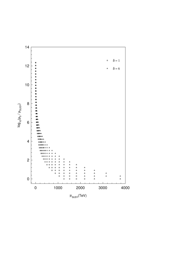
Figure 1: The ratio $\mu_{0}/\mu_{SUSY}$ plotted against various SUSY breaking scales, $\mu_{SUSY}$. Only results within $1\sigma$ of $\alpha_{3}\left(M_{Z}\right)$ are presented. Unification is spoiled for points lying outside the corresponding bands.

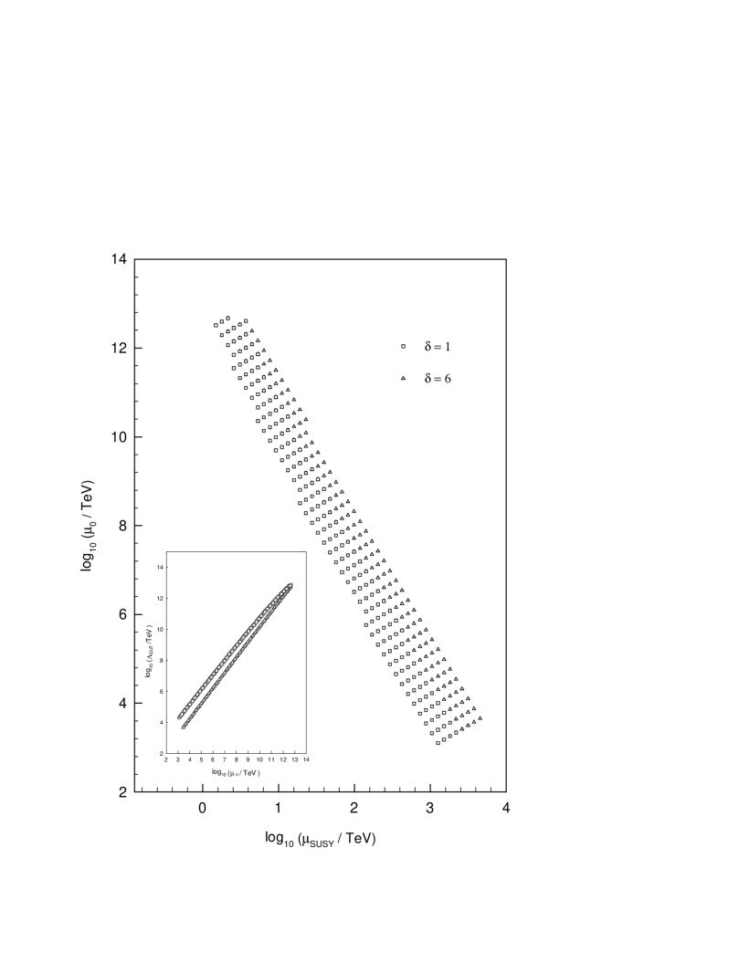
Figure 2: Scattered plot of the allowed compactification scales, $\mu_{0}$, for various SUSY breaking scales, $\mu_{SUSY}$. Only results within $1\sigma$ of $\alpha_{3}\left(M_{Z}\right)$ are presented. The same set of points as for the previous plot was used. Unification is spoiled for points lying outside the corresponding bands. The inset figure gives the unification scale against the compactification scale.

In Fig. 1 we plot the ratio $R=\mbox{log}_{10}\left({\mu_{SUSY}/\mu_{0}}\right)$ against $\mu_{SUSY}$. The vertical and horizontal spreads in the figure represent the ranges for which we get a solution at the $1\sigma$ range of $\alpha_{3}\left(M_{Z}\right)$. As a general feature, as the SUSY breaking scale increases, the compactification scale needed for unification decreases, a ratio of approximately $1$ being obtained around $\mu_{SUSY}\approx 1\times 10^{3}\>$TeV. This corresponds to the situation in which supersymmetry is broken as soon as the extra dimensions compactify. The same result is shown in Fig. 2 where $\mu_{0}$ is plotted against $\mu_{SUSY}$. The bands correspond to the regions in the plane for which unification is achieved within $1\sigma$ range of $\alpha_{3}\left(M_{Z}\right)$. It is interesting to note that for the unification band $\mu_{0}$ is approximately proportional to $\mu_{SUSY}^{-3}$. For this case, our results are in agreement with [8]. It can be concluded that there are no solutions leading to both $\mu_{SUSY}$ and $\mu_{0}$ in the $100\>$TeV or less range. Allowing $\eta\geq 1$ generations of matter fields to live in the $(4+\delta)$-dimensional space drives the unified coupling $\alpha_{GUT}$ towards higher values while preserving unification (in agreement with previous works).

4 One compactification scale scenario with $\mu_{SUSY}\geq\mu_{0}$

In this section we consider the posibility that the supersymmetry breaking occurs at a scale higher than the compactification scale, $\mu_{SUSY}\geq\mu_{0}$. For energies in the range $\mu_{0}\leq\mu\leq\mu_{SUSY}$ the theory is nonsupersymmetric but the gauge and Higgs sectors of SM along with $\eta$ generations of matter fields exhibit KK excitations. The corresponding contributions to the running are given by

$$\tilde{b}_{i}^{SM}=\left(1/10,-41/6,-21/2\right)+\eta\left(8/3,8/3,8/3\right).$$

At $\mu_{SUSY}$ the theory becomes supersymmetric and additional KK excitations of the sparticles lead to

$$\tilde{b}_{i}^{MSSM}=\left(3/5,-3,-6\right)+\eta\left(4,4,4\right).$$

For the numerical analysis we choose various compactification scales $\mu_{0}$ (starting in the TeV range) and search for SUSY breaking scales that lead to acceptable predictions for $\alpha_{3}\left(M_{Z}\right)$ (within $1\sigma$ of the central experimental value).

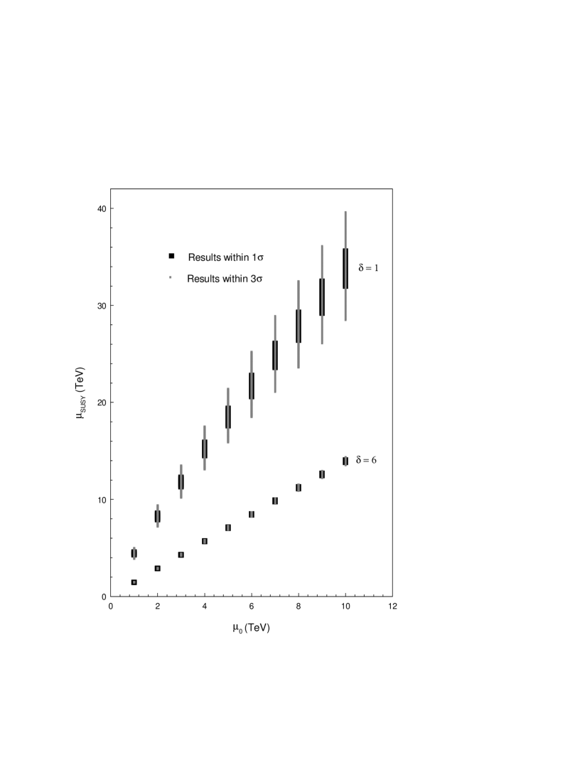
Figure 3: Allowed values of SUSY breaking scale, $\mu_{SUSY}$, for various choices of $\mu_{0}$ in a scenario with $\mu_{0}<\mu_{SUSY}$. Results within $1\sigma$ and $3\sigma$ of $\alpha_{3}\left(M_{Z}\right)$ are presented, for $\delta=1$ and $\delta=6$. Unification is spoiled if $\mu_{SUSY}$ lies outside the corresponding vertical spreads shown in the plot.

For the simplest case, $\eta=0$, the results are shown in Fig. 3 where the allowed values of $\mu_{SUSY}$ are plotted against the corresponding compactification scale $\mu_{0}$, for $\delta=1$ and $\delta=6$. Relevant numerical results are presented in Table 2.

As a generic feature, each compactification scale corresponds to a specific range of $\mu_{SUSY}$ that are needed for unification and are consistent with low-energy experimental data. The length of these intervals is, of course, determined by our requirement of $1\sigma$ (or $3\sigma$) agreement with the experimental value of $\alpha_{3}\left(M_{Z}\right)$ but it is found to increase with $\mu_{0}$. The fact that the upper bound of these ranges is finite shows that, within this model, supersymmetry is in fact needed for unification. Unification cannot occur within the SM spectrum. This was also noticed in [7] for the case $\mu_{SUSY}<\mu_{0}$.

This scenario is particularly appealing from the experimental point of view. Ignoring possible constraints on $\mu_{0}$ we consider a compactification scale as low as $\mu_{0}=1\>$TeV which enforces $\mu_{SUSY}=4.5\>$TeV and $\mu_{SUSY}=1.46\>$TeV for $\delta=1$ and $\delta=6$, respectively. This leads to unification at $\Lambda=75.2\>$TeV for $\delta=1$ and $\Lambda=2.68\>$TeV for $\delta=6$. A more realistic case would be $\mu_{0}=3\>$TeV, $\mu_{SUSY}=11.9\>$TeV with unification at $\Lambda=198\>$TeV for $\delta=1$ or $\mu_{SUSY}=4.3\>$TeV with unification at $\Lambda=7.86\>$TeV for $\delta=6$. Needless to say, these cases are well within the LHC reach and can be investigated at future experiments. The case $\eta=3$, not present in Table 2, led to negative unified coupling for the range of $\mu_{0}$ shown in Fig. 3.

Let us point out one caveat in the scenario presented. We have included only the one-loop contribution to the evolution of the couplings in the energy scale $\mu>\mu_{0}$. The corrections to the power-law evolution of the couplings due to the contribution of higher loops are small if the theory is supersymmetric, as shown in [14]. Thus in our scenario these corrections are small in the region $\mu_{SUSY}<\mu<\Lambda$. However, it is possible that such corrections could significantly affect our results in the region $\mu_{0}<\mu<\mu_{SUSY}$ due to the absence of supersymmetry in this region. This is especially true because realistically, the SUSY particles are not expected to be degenerate in mass at $\mu_{SUSY}$. Since in the region $\mu_{0}<\mu<\mu_{SUSY}$ the running of the couplings is approximately power law, the effect of the separate thresholds on the running, in principle, may be greater than in the logarithmic case. However, in the absence of a complete theory, it is not possible to calculate such effects. We note that this problem does not appear for $\mu_{0}\approx\mu_{SUSY}\approx 10^{3}$ TeV for which we do get unification of the gauge couplings.

We conclude this section with a few remarks. It was suggested in the literature [7] that the compactification scale could be identified with the SUSY breaking scale. Our results in this section and Sec. 3 indicate that, if this is the case, then this common scale cannot be lower than $10^{6}\>$GeV (around $10^{6}\>$Gev the ratio $\mu_{SUSY}/\mu_{0}$ required for unification approaches $1$ in both scenarios).

One question needs to be addressed here. Does string theory allow a scenario in which the compactification scale is lower than the SUSY breaking scale? In this case, SUSY has to be broken in a higher dimension before compactification. There are several possibilities for that to happen. One possibility is a string solution in which SUSY is broken at the string level. In general, non-SUSY string solutions are unstable. String theory prefers vacua which are supersymmetric. Dilaton and other modulii tend to run away to infinity, and restore SUSY. However, given the reach complexities and possibilities in string theory, such a scenario can not be ruled out. A second possibility is the gaugino condensation in higher dimensional gauge theory. The gauge coupling could be of the order of unity, causing gaugino condensation and breaking $N=2$ (or even $N=1$) SUSY, before compactification to four dimensions. Yet another possibility is that the SM particles (plus their SUSY partners) live in a non-Bogomol’nyi-Prasad-Sommerfield (BPS) brane which is stable but does not preserve supersymmetry at all [13]. Thus, we conclude that a scenario with $\mu_{SUSY}>\mu_{0}$ is not totally crazy, although such a scenario is probably not as well motivated as the $\mu_{SUSY}<\mu_{0}$ case.

5 Two scale compactification scenarios

In the analysis of Sec. 3 and 4 we assumed that the compactification of the extra dimensions takes place at a single mass scale, $\mu_{0}$. However, the possibility exists that the different extra dimensions compactify at different mass scales. Also, particles with different gauge quantum numbers may belong to different D branes associated with different compactification scales. This section is devoted to numerical analyses of such scenarios with two different mass scales, $\mu_{10}$ and $\mu_{20}$ with $\mu_{10}<\mu_{20}$. In these models the MSSM spectrum (or only a subset of it) is split up into two parts, with the first part developing KK excitations at the first compactification scale $\mu_{10}$ and with the remainder contributing only after the second scale $\mu_{20}$ is crossed.

In all the subsequent cases the SUSY breaking scale is assumed to be lower than $\mu_{10}$. For practical purposes we restrict ourselves to compactification scales $\mu_{10}$ that are within the LHC reach and to $\delta=1$ extra dimensions. Only results that lead to predictions of $\alpha_{3}(M_{Z})$ within $1\sigma$ of the central experimental value are presented.

In what follows we consider several scenarios in which the splitting of the MSSM gauge sector is based on color. Relevant numerical results for these models are presented in Table 4 and the $\beta$-function coefficients corresponding to the two compactification scales for the cases A, B, C, D presented below, are given by

$$\tilde{b}_{i}^{\left(10\right)} = \left(0,0,-6\right),$$ (6)

$$\tilde{b}_{i}^{\left(20\right)} = \left(0,-4,-6\right)+\eta\left(4,4,4,\right)$$

with the appropriate choice of $\eta$.
Case A
$\mu_{10}\rightarrow$ SU(3)
$\mu_{20}\rightarrow$ SU(3)$\otimes$SU(2)$\otimes$U(1)
The notation is that only the gluons (along with their SUSY partners) develop KK excitations at $\mu_{10}$, while the full MSSM gauge sector contribute above $\mu_{20}$. The $\beta$-function coefficients are given by Eq. 6 with $\eta=0$. For SUSY breaking scales in the TeV range and $\mu_{10}$ within the reach of LHC ($\leq 14\>$TeV), a ratio $\mu_{20}/\mu_{10}$ of about 7 is needed in order to achieve unification [with the prediction for $\alpha_{3}(M_{Z})$ within $1\sigma$ of the central experimental value]. The unification scale is as low as $4\times 10^{2}\>$TeV. Note that for this scenario the value of the couplings at the unification scale ($\alpha_{GUT}\approx 0.015$) is significantly smaller than $\alpha_{3}\left(M_{Z}\right)$ and well within the perturbative regime. As a general feature, attempts to bring the compactification scale $\mu_{10}$ down to $\mu_{SUSY}$ (at fixed $\mu_{20}/\mu_{10}$) tend to drive the unified coupling towards higher values.
Case B
$\mu_{10}\rightarrow$ SU(3),
$\mu_{20}\rightarrow$ SU(3)$\otimes$SU(2)$\otimes$U(1)$\;\oplus\;1\>\mbox{generation of matter fields}$
[$\eta=1$ in Eq. 6]. The addition of $\eta=1$ generation of matter fields at $\mu_{10}$ preserves unification while increasing the coupling at the unification scale ($\alpha_{GUT}\approx 0.032$). This case shares all the features of the previous one.
Case C
$\mu_{10}\rightarrow$ SU(3),
$\mu_{20}\rightarrow$ SU(3)$\otimes$SU(2)$\otimes$U(1)$\;\oplus\;2\>\mbox{generations of matter fields}$
[$\eta=2$ in Eq. 6]. With an MSSM spectrum at the TeV scale we found that this scenario does not lead to unification for $\mu_{10}$ within the LHC reach [although a mathematical unification is achieved, either the unified coupling $\alpha_{GUT}$ has unphysical values or the prediction for $\alpha_{3}(M_{Z})$ is outside $3\sigma$ of the experimental value]. However, extending the range of $\mu_{10}$ beyond the reach of LHC we found that unification can be achieved for $\mu_{10}\geq 5\times 10^{2}\>\mbox{TeV}$ and only for $\mu_{20}/\mu_{10}\approx 5.5$. The unification scale can be as low as $\Lambda=7.8\times 10^{4}\>\mbox{TeV}$ and the unified coupling is in the perturbative regime.
Case D
$\mu_{10}\rightarrow$ SU(3),
$\mu_{20}\rightarrow$ SU(3)$\otimes$SU(2)$\otimes$U(1)$\;\oplus\;3\>\mbox{generations of matter fields}$
[$\eta=3$ in Eq. 6]. This case is similar to Case C. A minimum compactification scale of $\mu_{10}\approx 7\times 10^{7}\>\mbox{TeV}$ and a ratio $\mu_{10}/\mu_{20}\approx 3.4$ are required for unification. Consequently, the unification scale is pushed towards about $\Lambda=3.1\times 10^{9}\>\mbox{TeV}$.

In Table 3 we list several other cases that were investigated but found not to give results of interest for future experiments at LHC.

Several conclusions can be drawn from the results above. Most importantly, the 2-scale scenarios allow for very low compactification scales (in the TeV range) even for the case in which the SUSY braking scale is lower than the compactification scale. This was not possible in one-scale scenarios. Moreover, results with $\mu_{SUSY}=\mu_{10}\>\approx$ few TeV are obtained, which encourages the identification of the SUSY breaking scale with the compactification scale. Specification of $\mu_{SUSY}$ along with the requirement that the first threshold is within the LHC reach, completely determined the second threshold as well as the unification scale [of course, with small variations determined by the error bar on the experimental value of $\alpha_{3}\left(M_{Z}\right)$].

6 Conclusions

In this work we have made a detailed investigation for the unification of the gauge couplings in MSSM with extra dimensions. We do not extend the gauge group or the field content (except for those required by the higher dimensions). In the previous studies, it was implicitly assumed that the SUSY breaks at four dimensions before the decompactification, and thus the scale of SUSY breaking, $\mu_{SUSY}$ is lower than the decompactification scale, $\mu_{0}$. In this case, it was observed that the three gauge couplings do not unify [satisfying the experimental range of $\alpha_{3}\left(M_{Z}\right)$] with both $\mu_{SUSY}$ and $\mu_{0}$ less than a few tens of a TeV. We have investigated several new scenarios for which the couplings unify with both $\mu_{SUSY}$ and $\mu_{0}$ in the few TeV scale. One particularly interesting scenario is when SUSY is broken at higher dimension [either through string dynamics or via gaugino condensation or in a non-Bogomol’nyi-Prasad-Sommerfield (BPS) brane] before decompactification, so that $\mu_{SUSY}>\mu_{0}$. In this case we obtained gauge coupling unification with both $\mu_{SUSY}$ and $\mu_{0}$ in the few TeV scale. This is very exciting, since for this scenario, LHC ($\sqrt{s}=14\>$TeV) will be able to probe experimentally the existence of these compact dimensions. The direct experimental test will be the observation of the low-lying KK resonance of SM particles, or the off-shell effect of these particles via the usual SM processes. A family of two scale compactification scenarios in which the MSSM gauge sector is split into its colored and uncolored subsets was also considered. It was found that with $\eta=0,1$ matter generations contributing above the second scale $\mu_{20}$, the unification can be achieved with both $\mu_{SUSY}$ and $\mu_{10}$ in the few TeV scale. In all cases unification can be achieved only for a specific narrow range of the ratio $\mu_{20}/\mu_{10}$.
Acknowledgments
We wish to thank K. S. Babu, J. Lykken and G. Gabadadze for useful discussions. This work was supported in part by the U.S. Department of Energy, Grant Number DE-FG03-98ER41076.

$\delta$	$\eta$	$\mu_{SUSY}$	$\mu_{0}$	$\alpha_{3}\left(M_{Z}\right)$	$\Lambda/\mu_{0}$	$\Lambda$	$\alpha_{GUT}$
$1$	$0$	$1.48\times 10^{3}$	$3.27\times 10^{15}$	$0.1208$	$1.91$	$6.25\times 10^{15}$	$0.0384$
$1$	$0$	$5.32\times 10^{3}$	$2.29\times 10^{13}$	$0.1208$	$5.14$	$1.18\times 10^{14}$	$0.0330$
$6$	$0$	$1.78\times 10^{3}$	$3.92\times 10^{15}$	$0.1206$	$1.20$	$4.71\times 10^{15}$	$0.0379$
$6$	$0$	$5.32\times 10^{3}$	$3.66\times 10^{14}$	$0.1193$	$1.37$	$5.00\times 10^{14}$	$0.0345$
$1$	$1$	$5.32\times 10^{3}$	$2.29\times 10^{13}$	$0.1208$	$5.14$	$1.18\times 10^{14}$	$0.0383$
$1$	$2$	$5.32\times 10^{3}$	$2.29\times 10^{13}$	$0.1208$	$5.14$	$1.18\times 10^{14}$	$0.0457$
$1$	$3$	$5.32\times 10^{3}$	$2.29\times 10^{13}$	$0.1208$	$5.14$	$1.18\times 10^{14}$	$0.0567$

Table 1: A few relevant numerical results for a one threshold scenario with $\mu_{SUSY}<\mu_{0}$. The behavior under changes of $\delta$ and $\eta$ is shown. All the mass scales are in GeV units. Relevant plots are presented in Fig. 1 and 2.

$\delta$	$\eta$	$\mu_{0}$	$\mu_{SUSY}/\mu_{0}$	$\mu_{SUSY}$	$\alpha_{3}\left(M_{Z}\right)$	$\Lambda/\mu_{0}$	$\Lambda$	$\alpha_{GUT}$
$1$	$0$	$1\times 10^{3}$	$4.5$	$4.5\times 10^{3}$	$0.1187$	$75.2$	$7.52\times 10^{4}$	$0.0197$
$1$	$0$	$2\times 10^{3}$	$4.2$	$8.3\times 10^{3}$	$0.1190$	$69.3$	$1.39\times 10^{5}$	$0.0199$
$1$	$0$	$3\times 10^{3}$	$4.0$	$1.19\times 10^{4}$	$0.1190$	$66.0$	$1.98\times 10^{5}$	$0.0200$
$1$	$0$	$4\times 10^{3}$	$3.8$	$1.53\times 10^{4}$	$0.1191$	$63.6$	$2.55\times 10^{5}$	$0.0200$
$1$	$0$	$5\times 10^{3}$	$3.8$	$1.86\times 10^{4}$	$0.1191$	$61.8$	$3.09\times 10^{5}$	$0.0201$
$1$	$0$	$7\times 10^{3}$	$3.6$	$2.50\times 10^{4}$	$0.1191$	$59.2$	$4.14\times 10^{5}$	$0.0201$
$1$	$0$	$9\times 10^{3}$	$3.5$	$3.11\times 10^{4}$	$0.1191$	$57.1$	$5.14\times 10^{5}$	$0.0202$
$6$	$0$	$1\times 10^{3}$	$1.46$	$1.46\times 10^{3}$	$0.1201$	$2.68$	$2.68\times 10^{3}$	$0.0187$
$6$	$0$	$2\times 10^{3}$	$1.45$	$2.89\times 10^{3}$	$0.1194$	$2.64$	$5.29\times 10^{3}$	$0.0188$
$6$	$0$	$3\times 10^{3}$	$1.43$	$4.3\times 10^{3}$	$0.1194$	$2.62$	$7.86\times 10^{3}$	$0.0189$
$6$	$0$	$4\times 10^{3}$	$1.43$	$5.71\times 10^{3}$	$0.1190$	$2.61$	$1.04\times 10^{4}$	$0.0190$
$6$	$0$	$5\times 10^{3}$	$1.42$	$7.10\times 10^{3}$	$0.1191$	$2.59$	$1.29\times 10^{4}$	$0.0190$
$6$	$0$	$7\times 10^{3}$	$1.41$	$9.86\times 10^{3}$	$0.1192$	$2.57$	$1.80\times 10^{4}$	$0.0191$
$6$	$0$	$9\times 10^{3}$	$1.40$	$1.26\times 10^{4}$	$0.1191$	$2.56$	$2.3\times 10^{4}$	$0.0192$
$1$	$1$	$1\times 10^{3}$	$4.5$	$4.5\times 10^{3}$	$0.1187$	$75.2$	$7.52\times 10^{4}$	$0.0332$
$1$	$2$	$1\times 10^{3}$	$4.5$	$4.5\times 10^{3}$	$0.1187$	$75.2$	$7.52\times 10^{4}$	$0.1040$
$6$	$1$	$1\times 10^{3}$	$1.46$	$1.46\times 10^{3}$	$0.1201$	$2.68$	$2.68\times 10^{3}$	$0.0327$
$6$	$2$	$1\times 10^{3}$	$1.46$	$1.46\times 10^{3}$	$0.1201$	$2.68$	$2.68\times 10^{3}$	$0.1300$

Table 2: Numerical results for the 1-scale scenario with $\mu_{SUSY}\geq\mu_{0}$. The compactification scales $\mu_{0}$ were taken as input and the allowed values of SUSY breaking scales were determined numerically. The behaviour under changes of $\delta$ and $\eta$ is shown. All the mass scales are in GeV. See Fig. 3 for a relevant plot.

$\mu_{10}$	SU(3)
$\mu_{20}$	SU(3)$\otimes$SU(2)$\otimes$U(1) $\oplus$ H
$\mu_{10}$	SU(3)
$\mu_{20}$	SU(3)$\otimes$SU(2)$\otimes$U(1) $\oplus$ 3(L, E)
$\mu_{10}$	SU(3)
$\mu_{20}$	SU(3)$\otimes$SU(2)$\otimes$U(1) $\oplus$ 3(L, Q)
$\mu_{10}$	SU(3) $\otimes$ U(1) $\oplus$ 3(U, D)
$\mu_{20}$	SU(3)$\otimes$SU(2)$\otimes$U(1) $\oplus$ 3(Q, U, D, L, E)
$\mu_{10}$	SU(3) $\otimes$ U(1) $\oplus$ 3(U, D)
$\mu_{20}$	SU(3)$\otimes$SU(2)$\otimes$U(1) $\oplus$ 3(Q, U, D, L, E) $\oplus$ H
$\mu_{10}$	SU(2)
$\mu_{20}$	SU(3)$\otimes$SU(2)$\otimes$U(1)
$\mu_{10}$	SU(2) $\otimes$ U(1) $\oplus$ 3(L, E) $\oplus$ H
$\mu_{20}$	SU(3)$\otimes$SU(2)$\otimes$U(1) $\oplus$ 3(Q, U, D, L, E) $\oplus$ H

Table 3: Two compactification scale scenarios which DO NOT lead to unification with both $\mu_{SUSY}$ and $\mu_{10}$ within the reach of LHC.

$\eta$	$\mu_{SUSY}$	$\mu_{10}$	$R$	$\mu_{20}$	$\alpha_{3}\left(M_{Z}\right)$	$\Lambda/\mu_{10}$	$\Lambda$	$\alpha_{GUT}$
0	$1\times 10^{3}$	$2\times 10^{3}$	$7.2$	$1.44\times 10^{4}$	$0.1189$	$212$	$4.23\times 10^{5}$	$0.0156$
0	$2\times 10^{3}$	$2\times 10^{3}$	$7.2$	$1.44\times 10^{4}$	$0.1176$	$211$	$4.21\times 10^{5}$	$0.0155$
0	$2\times 10^{3}$	$4\times 10^{3}$	$7.2$	$2.88\times 10^{4}$	$0.1196$	$207$	$8.28\times 10^{5}$	$0.0157$
0	$2\times 10^{3}$	$6\times 10^{3}$	$7.2$	$4.32\times 10^{4}$	$0.1209$	$205$	$1.23\times 10^{6}$	$0.0158$
0	$3\times 10^{3}$	$3\times 10^{3}$	$7.2$	$2.16\times 10^{4}$	$0.1179$	$208$	$6.23\times 10^{5}$	$0.0156$
0	$3\times 10^{3}$	$5\times 10^{3}$	$7.2$	$3.60\times 10^{4}$	$0.1195$	$205$	$1.03\times 10^{6}$	$0.0157$
0	$3\times 10^{3}$	$7\times 10^{3}$	$7.2$	$5.04\times 10^{4}$	$0.1205$	$204$	$1.43\times 10^{6}$	$0.0158$
0	$5\times 10^{3}$	$5\times 10^{3}$	$7.2$	$3.60\times 10^{4}$	$0.1184$	$205$	$1.02\times 10^{6}$	$0.0157$
0	$5\times 10^{3}$	$7\times 10^{3}$	$7.2$	$5.04\times 10^{4}$	$0.1194$	$203$	$1.42\times 10^{6}$	$0.0158$
0	$5\times 10^{3}$	$9\times 10^{3}$	$7.2$	$6.48\times 10^{4}$	$0.1202$	$202$	$1.81\times 10^{6}$	$0.0158$
1	$1\times 10^{3}$	$2\times 10^{3}$	$7.2$	$1.44\times 10^{4}$	$0.1189$	$212$	$4.23\times 10^{5}$	$0.0332$
1	$2\times 10^{3}$	$2\times 10^{3}$	$7.2$	$1.44\times 10^{4}$	$0.1176$	$211$	$4.21\times 10^{5}$	$0.0327$
1	$2\times 10^{3}$	$4\times 10^{3}$	$7.2$	$2.88\times 10^{4}$	$0.1196$	$207$	$8.28\times 10^{5}$	$0.0329$
1	$2\times 10^{3}$	$6\times 10^{3}$	$7.2$	$4.32\times 10^{4}$	$0.1209$	$205$	$1.23\times 10^{6}$	$0.0329$
1	$3\times 10^{3}$	$3\times 10^{3}$	$7.2$	$2.16\times 10^{4}$	$0.1179$	$208$	$6.23\times 10^{5}$	$0.0325$
1	$3\times 10^{3}$	$5\times 10^{3}$	$7.2$	$3.60\times 10^{4}$	$0.1195$	$205$	$1.03\times 10^{6}$	$0.0326$
1	$3\times 10^{3}$	$7\times 10^{3}$	$7.2$	$5.04\times 10^{4}$	$0.1205$	$204$	$1.43\times 10^{6}$	$0.0327$
1	$5\times 10^{3}$	$5\times 10^{3}$	$7.2$	$3.60\times 10^{4}$	$0.1184$	$205$	$1.02\times 10^{6}$	$0.0322$
1	$5\times 10^{3}$	$7\times 10^{3}$	$7.2$	$5.04\times 10^{4}$	$0.1194$	$203$	$1.42\times 10^{6}$	$0.0323$
1	$5\times 10^{3}$	$9\times 10^{3}$	$7.2$	$6.48\times 10^{4}$	$0.1202$	$202$	$1.81\times 10^{6}$	$0.0324$
2	$3\times 10^{3}$	$3.1\times 10^{7}$	$5.1$	$1.55\times 10^{8}$	$0.1174$	$99$	$3.04\times 10^{9}$	$0.1364$
2	$3\times 10^{3}$	$5.3\times 10^{7}$	$5.1$	$2.69\times 10^{8}$	$0.1190$	$98$	$5.15\times 10^{9}$	$0.1302$
2	$3\times 10^{3}$	$9.1\times 10^{7}$	$5.1$	$4.64\times 10^{8}$	$0.1206$	$96$	$8.73\times 10^{9}$	$0.1244$
2	$3\times 10^{3}$	$5.5\times 10^{5}$	$6$	$3.31\times 10^{6}$	$0.1175$	$142$	$7.81\times 10^{7}$	$0.3285$
2	$3\times 10^{3}$	$9.5\times 10^{5}$	$6$	$5.72\times 10^{6}$	$0.1191$	$139$	$1.33\times 10^{8}$	$0.2935$
2	$3\times 10^{3}$	$1.7\times 10^{6}$	$6$	$9.89\times 10^{6}$	$0.1208$	$137$	$2.26\times 10^{8}$	$0.2652$
3	$3\times 10^{3}$	$4.8\times 10^{11}$	$3$	$1.43\times 10^{12}$	$0.1177$	$30$	$1.4\times 10^{13}$	$0.1386$
3	$3\times 10^{3}$	$8.2\times 10^{11}$	$3$	$2.27\times 10^{12}$	$0.1193$	$29$	$2.4\times 10^{13}$	$0.1248$
3	$3\times 10^{3}$	$1.4\times 10^{12}$	$3$	$4.27\times 10^{12}$	$0.1209$	$28$	$3.9\times 10^{13}$	$0.1135$
3	$3\times 10^{3}$	$7.7\times 10^{10}$	$3.4$	$2.62\times 10^{11}$	$0.1177$	$40$	$3.1\times 10^{12}$	$0.3127$
3	$3\times 10^{3}$	$9.2\times 10^{10}$	$3.4$	$3.14\times 10^{11}$	$0.1183$	$40$	$3.7\times 10^{12}$	$0.2884$
3	$3\times 10^{3}$	$1.3\times 10^{11}$	$3.4$	$4.53\times 10^{11}$	$0.1193$	$39$	$5.2\times 10^{12}$	$0.2497$

Table 4: Numerical results for two scale compactification scenarios. The cases $\eta=0,1,2,3$ correspond to cases A,B,C,D respectively and $R=\mu_{20}/\mu_{10}$. The number of extra dimensions is $\delta=1$ and the mass scales are in GeV.

References

- [1] E. Witten, Nucl. Phys. B471, 135 (1996).
- [2] J. Lykken, Phys. Rev. D 54, 3693 (1996).
- [3] I. Antoniadis, Phys. Lett. B 246, 337 (1990); I. Antoniadis, K. Benakli, and M. Quiros, ibid. 331, 313 (1994).
- [4] N. Arkani-Hamed, S. Dimopoulos, and G. Dvali, Phys. Lett. B 429, 263 (1998).
- [5] N. Arkani-Hamed, S. Dimopoulos, and G. Dvali, Phys. Rev. D 59, 086004 (1999); I. Antoniadis, N. Arkani-Hamed, S. Dimopoulos, and G. Dvali, Phys. Lett. B 436, 257 (1998); N. Arkani-Hamed, S. Dimopoulos, and J. March-Russel, Phys. Rev. D (to be published), hep-th/9809124; S. Cullen and M. Perelstein, Phys. Rev. Lett. 83, 268 (1999) ; L.G. Hall and D. Smith, Phys. Rev. D 60, 085 008 (1999); V. Barger, T. Han, C. Kao, and R.-J. Zhang, Phys. Lett. B 461, 34 (1999).
- [6] For example see: E.A. Mirabelli, M. Perelstein, and M.E. Perskin, Phys. Rev. Lett. 82, 2236 (1999); G.F. Giudice, R. Rattazzi, and J.D. Wells, Nucl. Phys. B554, 3 (1999); T. Han, J.D. Lykken, and R.-J. Zhang, Phys. Rev. D 59, 105006 (1999); J.E. Hewett, Phys. Rev. Lett. 82, 4765 (1999); G.Shiu and S.H.H. Tye, Phys. Rev. D bf 58,106007 (1998); T. Banks, A. Nelson, and M. Dine, J. High Energy Phys. 06, 014 (1999); P. Mathews, S. Raychaudhuri, and S. Sridhar, Phys Lett. B 450, 343 (1999), hep-ph/9904232; T.G. Rizzo, Phys. Rev. D 59, 115010 (1999); C. Balazs, H.-J. He, W.W. Repko, C.-P. Yan, and D.A. Dicus, Phys. Rev. Lett. 83,2112 (1999); I. Antoniadis, K. Benakli and M. Quiros, Phys. Lett. B 360, 176 (1999); P. Nath, Y. Yamada and M. Yamaguchi, ibid. 466, 100 (1999); W.J. Marciano, Phys. Rev. D 60, 09006 (1999); T. Han, D. Rainwater, and D. Zepenfield, Phys. Lett. B 463, 93 (1999); K. Aghase and N. G. Deshpande, ibid. 456, 60 (1999); G. Shiu, R.Shrock and S.H.H. Tye, ibid. 458, 274 (1999); K. Cheung and Y. Keung, Phys. Rev. D. 60, 112003 (1999)
- [7] K.R. Dienes, E. Dudas and T. Ghergheta, Phys. Lett. B 436, 55 (1998), ibid Nucl. Phys. B537, 47 (1999).
- [8] D. Ghilencea and G. C. Ross, Phys. Lett. B 442, 165 (1998).
- [9] K.R. Dienes, E. Dudas, and T. Gherghetta, hep-ph/9807522.
- [10] C.D. Carone, Phys.Lett. B 454, 70 (1999); P.H. Frampton and A. Rasin, ibid. 460, 313 (1999); A. Delgado and M. Quiros, Nucl. Phys. B559, 235 (1999).
- [11] A. Perez-Lorenzana and R.N. Mohapatra, hep-ph/9905137
- [12] H.-C. Cheng, B. A. Dobrescu and C.T. Hill, hep-ph/9906327, K. Huitu and T. Kobayashi, hep-ph/9906431
- [13] For example, see the review by A. Sen, hep-th/9904207, see also G. Dvali and M. Shifman, hep-ph/9904021.
- [14] Z. Kakushadze and T. R. Taylor, Nucl. Phys. B562, 78 (1999).