Peripheral Meson Model of Deep Inelastic

Rapidity Gap Events

Hung Jung Lu^a, Rodrigo Rivera^b and Ivan Schmidt^b†

^aKnowledge Adventure Inc., 1311 Grand Central Ave., Glendale, CA 91201, U.S.A.

^bDepartamento de Física, Universidad Técnica Federico Santa María,

Casilla 110-V, Valparaíso, Chile

^†e-mail: ischmidt@fis.utfsm.cl

Abstract

We show that a peripheral meson model can explain the large deep inelastic electron-proton scattering rapidity gap events observed at HERA.

PACS numbers: 13.60.Hb, 14.40.-n

1 Introduction

Consider a proton at rest. Surrounding this proton there is a cloud of mesons ($\pi,\rho,\omega,\phi$, f2, etc…), which is fairly diluted at a distance that is large compared to the proton radius. That is, every meson is well separated from the rest of the mesons. Furthermore, due to the low density of mesons, nuclear models of proton-meson interactions should work on this regime, making perturbation theory a valid approximation, because the expansions are not only on the powers of the proton-meson effective coupling, but the series is also suppressed by powers of the product between the meson mass and the physical meson-proton distance[1].

Now let us imagine a high $Q^{2}$ virtual photon in deep inelastic scattering, which due to the high $Q^{2}$ has vanishing size. Sometimes this photon will collide with the proton core, which constitutes a typical deep inelastic scattering events. but in other instances it scatters off one of the isolated mesons in the disperse meson cloud. The photon then breaks down the meson, and the pieces of the broken meson fragment independently of what happens to the proton. In fact, if the meson is far away, and if for instance the meson is a neutral pion, the most probable outcome is that the proton core will not be affected by the interaction between the photon and the meson, and after the meson is broken, the proton core will maintain its identity as a proton. Of course, if on the other hand the meson is charged, or if the core suffers the effects from the hard interaction, the proton can get excited into final states such as neutron, a $\Delta$(-,0,+,++), etc.

The basic picture is then the following: after the interaction we have a broken meson and a baryon which basically does not move much. Now, let us boost this picture to the laboratory system of HERA. What we see is that the proton looses very little momentum and continues down the beampipe, and the meson fragments are observed in the central rapidity zone, with a rapidity gap between the meson fragments and the proton direction (forward direction of beampipe).

This picture we just presented gives a natural simple explanation of the rapidity gap events observed at HERA[2]. It is the purpose of this paper to show that this is indeed the case, doing the corresponding calculation in detail.

The peripheral meson model we are considering here is different from the Pomeron exchange model[3], which is the one that is usually ascribed to these large rapidity gap events. In fact, these two models give quite different predictions. Specifically the meson model predicts the presence of several excited baryonic states, besides the proton, in the forward direction of HERA; while the Pomeron model predicts that only the proton will be present there. Therefore future measurements in these region should be able to clearly distinguish between the two models.

2 The Model

The model we are considering is based on the diagram shown in Fig. 1, where a rapidity gap appears between the baryonic beampipe system $N^{*}$ and the hadrons comprising system $X$.

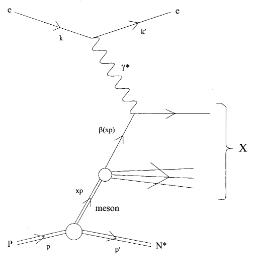
Figure 1: Diagram for the process $e(k)+p(p)\to e(k^{\prime})+N^{*}(p^{\prime})+X$, in which a meson produces a rapidity gap between $N^{*}$ and $X$.

The measured diffractive structure function is in general a function of three variables, which can be taken as the photon momentum transfer $Q^{2}$, the Bjorken variable $Q^{2}/2p\cdot q$, and the variable $\beta=Q^{2}/2q\cdot(p-p^{\prime})$. Since the cross section is dominated by small $t=(p-p^{\prime})^{2}$ values ($\arrowvert t\arrowvert\ll Q^{2},M_{X}^{2}$), both $\beta$ and the variable $x=q\cdot(p-p^{\prime})/p\cdot q$ can be reconstructed from the measured quantities $x_{Bj}=x\beta$ and $M_{X}^{2}/Q^{2}=(1-\beta)/\beta$.

Therefore the whole process depicted in Fig. 1 implies that the diffractive structure function can be expressed as:

$$F_{2}^{d}(x_{Bj},Q^{2},\beta)=\sum_{m}f_{m/p}(x,Q^{2})F_{2}^{m}(\beta,Q^{2}).$$ (1)

Here $f_{m/p}(x,Q^{2})$ is the probability of finding the emitted meson carrying a fraction $x$ of the proton momentum, and $F_{2}^{m}(\beta,Q^{2})$ is the usual deep inelastic structure function of the corresponding meson. Then the photon scatters on a quark that carries a fraction $\beta$ of the meson momentum. Although in principle the sum is over all mesons, we will see below that a limited number actually contributes to the process. Notice that we are in fact using an equivalent particle approximation, in which the process is dominated by the region in which the particle (in this case the meson) is close to its mass shell.

Since we are not looking into spin effects, for simplicity we will assume that the partonic distributions inside a meson are not very different form those inside a pion[4]. Therefore our task is to work out expressions for the different distribution functions of mesons inside a proton.

The equivalent meson approximation allows for a separation of the amplitude for the whole process into an amplitude for a transition to a baryon $N^{*}$ and a near mass-shell meson, followed by the amplitude for the interaction of the meson with a particle $a$ (in our case the off-shell photon). Using this it is easy to show that the external and internal cross sections are related through:

$$d\sigma_{ap}=f_{m/p}(x,\tilde{K}^{2})\ dx\ d\sigma_{a\pi},$$ (2)

where the meson distribution inside a proton is then:

$$f_{m/p}(x,\tilde{K}^{2})=\intop_{x^{2}M_{p}^{2}\over 1-x}^{\tilde{K}^{2}}{x\over 16\pi^{2}}{\mid M_{mp}\mid^{2}\over(K^{2}+m_{m}^{2})^{2}}dK^{2}.$$ (3)

Here $\mid M_{mp}\mid^{2}$ is the squared unpolarized amplitude for meson-$N^{*}$ emission (summed over final spins of the meson, and averaged over initial spins of the proton), $t=-K^{2}$ is the momentum squared of the pion, and $m_{m}$ and $M_{p}$ are the meson and proton masses respectively. $\tilde{K}^{2}$ is a momentum cut-off scale inherent to the formalism of equivalent particle approximation, and in our case it represents a parameter that fixes the separation of the pion from the color field of the proton. So we expect that its value be of the order of $\Lambda_{QCD}$ or less, although in our calculation we will leave it as an adjustable parameter. Notice that, as expected, the integral is dominated by small $t$ values.

The amplitude $M_{mp}$ contains a baryon-meson-baryon form factor, which can be taken as[5]:

$$F(K^{2})=\left(\Lambda^{2}-m_{m}^{2}\over\Lambda^{2}+K^{2}\right)^{n},$$ (4)

where $\Lambda$ is a parameter and $m_{m}$ is the meson mass. In the parameterization of Ref. [5], the exponent $n$ is equal to $1$, except for the $\rho N\Delta$ case, where $n=2$.[5]

2.1 Pion distribution inside the proton:

We start with the lightest meson, the pion, in which case our general formula is exact. The amplitude for the whole process $M_{ap}$ is related to the pion-$a$ subprocess through:

$$iM_{ap}=<p^{\prime}\mid-ig_{\pi NN}\gamma_{5}\mid p>{i\over t-m_{\pi}^{2}}iM_{a\pi}F_{\pi NN}(K^{2}),$$ (5)

where $p$ and $p^{\prime}$ are the initial and final proton momenta, $g_{\pi NN}$ is the proton-pion coupling constant, and $F_{\pi NN}(K^{2})$ is the proton-pion form factor. We are here considering the $\pi_{0}$ case, and for $\pi_{\pm}$ we simply need to multiply $M_{ap}$ by an isospin factor of $\sqrt{2}$. Then after squaring this result we get:

$$\mid M_{\pi pp}\mid^{2}=g_{\pi NN}^{2}Q^{2}\mid F_{\pi NN}\mid^{2}.$$ (6)

Hence the pion distribution inside a proton is then:

$$f_{p\to\pi_{0}p}(x,\tilde{K}^{2})=x\intop_{x^{2}M_{p}^{2}\over 1-x}^{\tilde{K}^{2}}{\alpha_{\pi NN}\over 4\pi}{K^{2}\over({K}^{2}+m_{\pi}^{2})^{2}}\big{\arrowvert}F_{\pi NN}(K^{2})\big{\arrowvert}^{2}dK^{2},$$ (7)

where $\alpha_{\pi NN}=g_{\pi NN}^{2}/4\pi$. At small $x$, the pion distribution is then proportional to $x$. That is, it will have a limited contribution for the events of our interest. The same is true for the transition $p\to\pi\Delta$, and also for and other scalar or pseudoscalar meson.

2.2 Vector meson distributions:

Here we will study the vector meson distributions, and show that these are the most important contributions at the small $x$ region of our interest. In fact, most of the effect comes from the omega meson (proton in the final state), and the rho (nucleon and delta isobars in final state).

We will need to generalize the equivalent photon approximation[6] to the meson case. In this paper we just quote the results, both for spin-1 and spin-2 particles. Details will be presented elsewhere[7].

(a) Omega Emission: The omega meson has purely vector interaction, so the matrix element for proton to proton-omega emission is:

$$iM_{\omega pp}=<p^{\prime}\mid-ig_{\omega NN}\ \gamma_{\mu}\mid p>F_{\omega NN}(K^{2})\epsilon^{\mu}.$$ (8)

After squaring, we get:

$$|M_{\omega pp}|^{2}={1\over 2}g_{\omega NN}^{2}|F_{\omega NN}(K^{2})|^{2}Tr\bigl{\{}(\hbox{p\kern-5.0pt\lower 1.29167pt\hbox{/}}^{\prime}+M_{p})\gamma^{\mu}(\hbox{p\kern-5.0pt\lower 1.29167pt\hbox{/}}+M_{p})\gamma^{\nu}\bigr{\}}\big{[}-g_{\mu\nu}+{K^{2}(K^{2}+{m}_{\omega}^{2})\over 4x^{2}m_{\omega}^{2}P^{4}}k^{\mu}k^{\nu}\big{]},$$

where the last factor comes from the completeness relation of the omega meson’s polarization vector, after making the equivalent meson approximation. The light-like vector $k$ is given by $k=(P,0,0,-P)$, where $P$ is just a frame choice parameter, which will not appear in the final answer. Taking the small $x$ and small $K^{2}$ limit, we get:

$$\mid M_{\omega pp}\mid^{2}=4g_{\omega NN}^{2}{K^{2}\over x^{2}}{(K^{2}+m_{\omega}^{2})\over m_{\omega}^{2}}|F_{\omega NN}(K^{2})|^{2}.$$ (9)

Introducing this result in our expression for the meson distribution we finally get:

$$f_{p\to\omega p}(x,\tilde{K}^{2})={g_{\omega NN}^{2}\over 4\pi^{2}x}\ \intop_{0}^{\tilde{K}^{2}}{K^{2}\mid F(K^{2})\mid^{2}\over m_{\omega}^{2}(K^{2}+m_{\omega}^{2})}dK^{2}.$$ (10)

(b) Rho emission: The rho meson has a vector interaction term and a “helicity-flipping” term. The matrix element for proton to proton-rho is:

$$iM_{\rho pp}=\bigl{\{}-ig_{\rho NN}<p^{\prime}\big{|}\gamma^{\mu}\big{|}p>-{f_{\rho NN}\over 2M_{p}}<p^{\prime}\big{|}\sigma^{\mu\nu}\big{|}p>q_{\nu}\bigr{\}}F_{\rho NN}(K^{2}).$$ (11)

For the proton to neutron-rho case an isospin factor of $\sqrt{2}$ should be inserted in the above expression. After squaring we get:

$$\big{|}M_{\rho pp}\big{|}^{2}={4K^{2}(K^{2}+m_{\rho}^{2})\over x^{2}m_{\rho}^{2}}\big{(}g_{\rho NN}^{2}+{f_{\rho NN}^{2}K^{2}\over 4M_{p}^{2}}\big{)}\big{|}F_{\rho NN}(K^{2})\big{|}^{2},$$ (12)

and therefore for the rho distribution the following result is obtained:

$$f_{p\to\rho_{0}p} = {\alpha_{\rho NN}^{(V)}\over\pi x}\intop_{0}^{\tilde{K}^{2}}{K^{2}\over m_{\rho}^{2}(K^{2}+m_{\rho}^{2})}\big{|}F_{\rho NN}{(K^{2})}^{2}\big{|}dK^{2}$$ (13)

$$+ {\alpha_{\rho NN}^{(T)}\over 4\pi x}\intop_{0}^{\tilde{K}^{2}}{K^{4}\over m_{\rho}^{2}M_{p}^{2}(K^{2}+m_{\rho}^{2})}\big{|}F_{\rho NN}(K^{2})\big{|}^{2}dK^{2},$$

where $\alpha_{\rho NN}^{(V)}=g_{\rho NN}^{2}/4\pi$ and $\alpha_{\rho NN}^{(T)}=f_{\rho NN}^{2}/4\pi$. Numerically it turns out that the helicity-flipping contribution is much smaller than the vector part contribution.

The proton can also emit a $\rho^{-}$ and a $\Delta^{++}$. The $p\to\rho^{0}\Delta^{+}$ transition probability is related to the previous one by an isospin factor of $2/3$, and the $p\to\rho^{+}\Delta^{0}$ by a factor of $1/3$. There are no $\sigma$ or $\omega$ meson coupling to the $p\to\Delta$ transition, because the spin of the proton is $1/2$, of the $\Delta$ is $3/2$, while the $\sigma$ and $\omega$ have spin zero.

The $N\Delta\rho$ emission matrix element can be written as:

$$i{f_{\rho N\Delta}\over m_{\rho}}\left[iq_{\mu}<\Delta^{\nu}\mid\gamma^{5}\gamma^{\mu}\mid p>\epsilon_{\nu}-iq_{\mu}<\Delta^{\mu}\mid\gamma^{5}\gamma^{\nu}\mid p>\epsilon_{\nu}\right]t_{\rho N\Delta},$$ (14)

where $t_{\rho N\Delta}=1,{2\over 3},{1\over 3}$ is the isospin factor mentioned above. Using the completeness relation for the isobar particle [8]:

$$\sum_{\lambda}u_{\mu}(\lambda){\overline{u}}_{\nu}(\lambda)={1\over 3}(\hbox{p\kern-5.0pt\lower 1.29167pt\hbox{/}}^{\prime}+m_{\Delta})\left[{2\over m_{\Delta}^{2}}p^{\prime}_{\mu}p^{\prime}_{\nu}-g_{\mu\nu}-\gamma_{\nu}\gamma_{\mu}+{\gamma_{\mu}p^{\prime}_{\nu}-\gamma_{\nu}p^{\prime}_{\mu}\over m_{\Delta}}\right],$$ (15)

and the completeness relation for the $\rho$ in the equivalent meson approximation, we get an expression for the emission matrix element squared whose value in the small $x$ limit is:

$$\mid M_{\rho p\Delta}\mid^{2}={2t_{\rho N\Delta}^{2}f_{\rho N\Delta}^{2}\over 3m_{\Delta}^{2}m_{\rho}^{4}x^{2}}K^{2}(K^{2}+m_{\rho}^{2})\big{[}K^{4}+(3m_{\Delta}^{2}+M_{p}^{2})K^{2}\big{]}\big{|}F_{\rho N\Delta}\big{|}^{2}.$$ (16)

So finally the distribution function becomes:

$$f_{p\rightarrow\rho\Delta}(x,\tilde{K}^{2})={t_{\rho N\Delta}^{2}\alpha_{\rho N\Delta}\over 6\pi m_{\Delta}^{2}m_{\rho}^{4}x}\intop\limits_{0}^{\tilde{K}^{2}}{K^{4}(K^{2}+3m_{\Delta}^{2}+M_{p}^{2})\over(K^{2}+m_{\rho}^{2})}\big{|}F_{\rho N\Delta}(K^{2})\big{|}^{2}dK^{2}$$ (17)

where $\alpha_{\rho N\Delta}=f_{\rho N\Delta}^{2}/4\pi$ and the isospin factor $t_{N\Delta\rho}^{2}=1,2/3,1/3$ for $p\rightarrow\rho^{-}\Delta^{++}$, $p\rightarrow\rho^{0}\Delta^{+}$, $p\rightarrow\rho^{+}\Delta^{0}$, respectively.

(c) $K^{*}$ Emission: Here the final state can be either a $\Sigma$ or a $\Lambda$. Only the latter gives a contribution comparable with those of the $\omega$ and $\rho$ cases. In the same way as before we get:

$$f_{p\to K^{*}\Lambda} = {\alpha_{K^{*}N\Lambda}^{(V)}\over\pi x}\intop_{0}^{\tilde{K}^{2}}{K^{2}\over m_{K^{*}}^{2}(K^{2}+m_{K^{*}}^{2})}|F_{K^{*}N\Lambda}{(K^{2})}|^{2}dK^{2}$$ (18)

$$+ {\alpha_{K^{*}N\Lambda}^{(t)}\over 4\pi x}\intop_{0}^{\tilde{K}^{2}}{K^{4}\over m_{K^{*}}^{2}M_{p}^{2}(K^{2}+m_{K^{*}}^{2})}\big{|}F_{K^{*}N\Lambda}(K^{2})\big{|}^{2}dK^{2},$$

where $\alpha_{K^{*}N\Lambda}^{(V)}=g_{K^{*}N\Lambda}^{2}/4\pi$ and $\alpha_{K^{*}N\Lambda}^{(T)}=f_{K^{*}N\Lambda}^{2}/4\pi$.

2.3 Spin 2 meson distributions

These contributions are progressively smaller due to the higher mass of the spin 2 particles. Thus we will only consider the lightest spin 2 particle, the $f_{2}(1270)$, and we will leave its coupling constant as an adjustable parameter.

The $f_{2}NN$ matrix element can be written as:

$$iM_{f_{2}NN}\ =\ {if_{f_{2}NN}\over 4m_{f_{2}}}<p^{\prime}\mid V^{\mu\nu}\mid p>\phi_{\mu\nu}F_{f_{2}NN}(K^{2}),$$ (19)

where the symmetric tensor $\phi_{\mu\nu}$ is the spin-2 particle field. The vertex $V^{\mu\nu}$ is[9]:

$$V^{\mu\nu}={4M_{p}\over s^{2}}s^{\mu}s^{\nu}+(s^{\mu}\gamma^{\nu}+s^{\nu}\gamma^{\nu}),$$ (20)

with $s^{\mu}=p^{\mu}+p^{\prime\mu}$.

After squaring, averaging over initial spins and summing over delta spins, we get:

$$\mid M_{f_{2}NN}\mid^{2}={f^{2}_{f_{2}NN}\over 32m^{2}_{f_{2}}}\Lambda_{\mu\nu,\rho\sigma}Tr\{(\hbox{p\kern-5.0pt\lower 1.29167pt\hbox{/}}^{\prime}+m)V^{\mu\nu}(\hbox{p\kern-5.0pt\lower 1.29167pt\hbox{/}}+m)V^{\rho\sigma}\}\ F_{f_{2}NN}(K^{2}),$$

where the $\Lambda_{\mu\nu,\rho\sigma}$ factor comes from the equivalent particle approximation, and is given by:

$$\Lambda_{\mu\nu,\rho\sigma} = {1\over 2}(g_{\mu\rho}g_{\nu\sigma}+g_{\mu\sigma}g_{\nu\rho})+{1\over 2}{K^{2}\over(2xP^{2})^{2}}$$

$$\times (g_{\mu\rho}k_{\nu}k_{\sigma}+g_{\mu\sigma}k_{\nu}k_{\rho}+g_{\nu\rho}k_{\mu}k_{\sigma}+g_{\nu\sigma}k_{\mu}k_{\rho})$$

$$+ {K^{4}\over(2xP^{2})^{4}}\left({1\over 2}-{2K^{2}\over m_{f}^{2}}+{K^{4}\over m_{f}^{4}}\right)k_{\mu}k_{\nu}k_{\rho}k_{\sigma}.$$

Thus, in the small $K^{2}$ and small $x$ limit we get:

$$|M_{f_{2}NN}|^{2}={4f_{f_{2}NN}^{2}\over m_{f_{2}}^{2}}{K^{4}\over x^{4}}\big{(}{1\over 2}-{2K^{2}\over m_{f}^{2}}+{K^{4}\over m_{f}^{2}}\big{)}{(16M_{p}^{2}+K^{2})\over(4M_{p}^{2}+K^{2})}|F_{f_{2}NN}(K^{2})|^{2},$$ (22)

and therefore we obtain for the $f_{2}$ distribution function:

$$f_{p\rightarrow f_{2}p}={f_{f_{2}NN}^{2}\over 4\pi^{2}m_{f}^{2}x^{3}}\intop\limits_{0}^{\tilde{K}^{2}}{K^{4}(16M_{p}^{2}+K^{2})\over(4M_{p}^{2}+K^{2})(K^{2}+m_{f}^{2})^{2}}\big{(}{1\over 2}-{2K^{2}\over m_{f}^{2}}+{K^{4}\over m_{f}^{4}})|F_{f_{2}NN}(K^{2})|^{2}dK^{2}.$$ (23)

2.4 Parton Distributions in Mesons

From the above calculations we have obtained various distribution functions $f_{m/p}(x,Q^{2})$ in the equivalent meson approximation. In order to compare our results in Eq. (1) with the experimental data from HERA[2], we need the parton distribution functions $F_{2}^{m}(\beta,Q^{2})$ for each of the mesons we have considered ($\pi^{0},\pi^{+},\rho^{-},\rho^{0},\rho^{+},K^{*+},f_{2})$.

The parton content of mesons is presently poorly known. Thus we will assume here that the valence, sea and strange quark distributions of all the mesons mimic the parton distributions of pions. For the pion’s distribution functions, we use the GRV parameterization[4]. Then each of the $F_{2}^{m}(x,Q^{2})$ can be written in terms of three independent functions: (1) the valence quark distribution: $xv^{\pi}(x,Q^{2})$, (2) the light sea-quark distribution: $x\overline{q}^{\pi}(x,Q^{2})$, and (3) the strange sea-quark distribution: $x\overline{s}^{\pi}(x,Q^{2})$. That is:

$$F_{m}^{2}(x,Q^{2})=C_{1}^{m}xv^{\pi}(x,Q^{2})+C_{2}^{m}x\overline{q}(x,Q^{2})+C_{3}^{m}x\overline{s}(x,Q^{2}).$$ (24)

The coefficients for the charged mesons $m=(\pi^{+},\rho^{-},\rho^{+})$ are $(C_{1}^{m},C_{2}^{m},C_{3}^{m})=({5\over 9},{10\over 9},{2\over 9})$, and for the neutral mesons $m=(\pi^{0},\rho^{0},f_{2})$ are $(C_{1}^{m},C_{2}^{m},C_{3}^{m})=({5\over 18},{10\over 9},{2\over 9})$. For the special case of the strange meson $K^{*+}$, for simplicity we will assume a parton distribution $F_{m}^{2}(x,Q^{2})$ similar to that of the charged mesons.

3 Results

There are three parameters in our model, namely, the momentum squared cut-off $\tilde{Q}^{2}$ (which should be around $\Lambda^{2}_{QCD}$), the tensor-meson coupling constant $\alpha_{f_{2}NN}={f_{f_{2}NN}^{2}\over 4\pi}$, and the form factor momentum cut-off scale $\Lambda_{f_{2}NN}$. We have chosen the values $\tilde{K}^{2}=0.048[GeV^{2}],f_{f_{2}NN}=4$, and $\Lambda_{f_{2}NN}=1.29[GeV]$.

Figure 2: Comparison between the predictions of the peripheral meson model and experimental data[2].

In Fig. 2 we compare the results of our model with the experimental data from HERA[2]. We have plotted the results for $F_{2}^{d}(x,Q^{2},\beta)$ for $Q^{2}=12,28,75[GeV^{2}]$ and $\beta=0.1,0.4,0.9$. Form the plots we can see that the x-dependence of $F_{2}^{d}(x,Q^{2},\beta)$ can be explained from the x-dependence of the equivalent meson content of the proton.

4 Conclusions

We have presented here an equivalent-meson model in order to explain the observed large rapidity gap events at HERA. We have seen that the peripheral meson content of the proton can explain the x-dependence of the measured $F_{2}^{m}(x,Q^{2},\beta)$ structure functions. Thus, from standard nuclear physics knowledge and the parton distribution of mesons, the essential features of this class of events can be explained. Our model implies the existence of interesting final states in the forward baryon, including helicity-flipping proton and isospin-changing states (e.g. $\Delta^{++}$) in the forward direction, which should be interesting to observe in large rapidity gap events.

Acknowledgments: We would like to thank Stanley J. Brodsky for helpful conversations. This work has been partially supported by Fondecyt (Chile) under grant 1990806 and by a Cátedra Presidencial (Chile). R. Rivera thanks Fundación Andes for a Doctoral grant.

References

- [1] See for example: R. Machleidt, in “Advances in Nuclear Physics”, Vol. 19, 189 (Plenum Press, 1989).
- [2] M. Derrick et al., Zeits. für Phys. C68, 569 (1995); C. Adloff et al., Zeits. für Phys. C76, 613 (1997).
- [3] See for example: M. Wüsthoff, Phys. Rev. D56, 4311 (1997), and references therein.
- [4] M. Glück, E. Reya and A. Vogt, Zeits. für Phys. C53, 651 (1992); M. Glück, E. Reya and I. Schienbein, preprint DO-TH 99/01, hep-ph/9903288.
- [5] B. Holzenkamp et al., Nucl. Phys. A500, 485 (1989).
- [6] See for example: V. M. Budnev et al., Phys. Rep. C15, 181 (1975).
- [7] H.-J. Lu, R. Rivera and I. Schmidt, in preparation.
- [8] O. Dumbrajs et al., Nucl. Phys. B216, 277 (1983).
- [9] K. V. Vasavada, Phys. Rev. D9, 1918 (1975).