Neutrino Physics

Abstract

These lectures describe some aspects of the physics of massive neutrinos. After a brief introduction of neutrinos in the Standard Model, I discuss possible patterns for their masses. In particular, I show how the presence of a large Majorana mass term for the right-handed neutrinos can engender tiny neutrino masses for the observed neutrinos. If neutrinos have mass, different flavors of neutrinos can oscillate into one another. To analyze this phenomena, I develop the relevant formalism for neutrino oscillations, both in vacuum and in matter. After reviewing the existing (negative) evidence for neutrino masses coming from direct searches, I discuss evidence for, and hints of, neutrino oscillations in the atmosphere, the sun, and at accelerators. Some of the theoretical implications of these results are emphasized. I close these lectures by briefly outlining future experiments which will shed further light on atmospheric, accelerator and solar neutrino oscillations. A pedagogical discussion of Dirac and Majorana masses is contained in an appendix.

I Neutrinos in the Standard Model

Neutrinos play a special role in the $SU(2)\times U(1)$ electroweak theory. While the left-handed neutrinos are part of $SU(2)$ doublets

$$L_{i}=\left(\begin{array}[]{c}\nu_{\ell_{i}}\\ \ell_{i}\end{array}\right)_{\rm L}~{},~{}~{}~{}~{}~{}~{}\ell_{i}=\{e,\mu,\tau\}~{},$$ (1)

the right-handed neutrinos are $SU(2)$ singlets. Since the electromagnetic charge and the $U(1)$ hypercharge differ by the value of the third component of weak isospin

$$Q=T_{3}+Y~{},$$ (2)

one sees that the right-handed neutrinos $(\nu_{\ell_{i}})_{\rm R}$ carry no $SU(2)\times U(1)$ quantum numbers. The above has two important experimental implications:

i) The neutrinos seen experimentally are those produced by the weak interactions. These neutrinos are purely left-handed.

ii) Because one cannot infer the existence of right-handed neutrinos from weak processes, the presence of $(\nu_{\ell_{i}})_{\rm R}$ can only be seen indirectly, most likely through the existence of neutrino masses. However, it should be noted that neutrino masses do not necessarily imply the existence of right-handed neutrinos.

Before discussing issues connected with neutrino masses, it is useful to summarize what we know about the left-handed neutrinos from their weak interactions. In the electroweak theory these neutrinos couple to the $Z$-boson in a universal fashion

$${\cal{L}}_{Z\nu\bar{\nu}}=\frac{e}{2\cos\theta_{W}\sin\theta_{W}}Z^{\mu}[J_{\mu}^{\rm NC}]_{\nu}~{},$$ (3)

where

$$[J_{\mu}^{\rm NC}]_{\nu}=\sum_{i}(\bar{\nu}_{\ell_{i}})_{\rm L}\gamma_{\mu}(\nu_{\ell_{i}})_{\rm L}~{}.$$ (4)

Precision studies of the $Z$-line shape allow the determination of the number of neutrino species $i$, since as this number increases so does the $Z$ total width. Each neutrino type (provided its mass $m_{\nu_{i}}\ll\frac{M_{Z}}{2}$) contributes the same amount to the $Z$-widthLEPEW

$$\Gamma(Z\to\nu_{\ell_{i}}\bar{\nu}_{\ell_{i}})=\frac{\sqrt{2}G_{F}M_{Z}^{3}}{24\pi}\rho~{}.$$ (5)

Here $G_{F}$ is the Fermi constant as determined in $\mu$-decayPDG and $\rho$ is related to the axial coupling of the charged leptons to the $Z$-boson: $\rho=(2g_{A}^{\ell})^{2}$. UsingLEPEW

$$g_{A}^{\ell}=-0.50102\pm 0.00030~{},$$ (6)

which is the average of the results obtained by the four LEP collaborations and SLD, one has numerically

$$\Gamma_{\nu}\equiv\Gamma(Z\to\nu_{\ell_{i}}\bar{\nu}_{\ell_{i}})=(167.06\pm 0.22)~{}{\rm MeV}~{}.$$ (7)

Using the above, the number of different neutrino species, $N_{\nu}$, can then be derived from the precision measurements of the $Z$ total width and of its partial width into hadrons and leptons using the (obvious) equation

$$\Gamma_{\rm tot}=\Gamma_{\rm had}+3\Gamma_{\rm lept}+N_{\nu}\Gamma_{\nu}~{}.$$ (8)

From a fit of the $Z$-line shape for $e^{+}e^{-}\to\mu^{+}\mu^{-}$ and $e^{+}e^{-}\to$ hadrons at LEP one can extract very accurate values for $\Gamma_{\rm tot},~{}\Gamma_{\rm lept}$ and $\Gamma_{\rm had}$:

$$\Gamma_{\rm tot} = (2.4939\pm 0.0024)~{}{\rm GeV}$$

$$\Gamma_{\rm lept} = (83.90\pm 0.1)~{}{\rm MeV}$$

$$\Gamma_{\rm had} = (1.7423\pm 0.0023)~{}{\rm GeV}~{}.$$ (9)

Whence it follows that the, so-called, invisible width is

$$\Gamma_{{\rm inv}}=N_{\nu}\Gamma_{\nu}=(499.9\pm 3.4)~{}{\rm MeV}$$ (10)

and thus one deduces for $N_{\nu}$—the number of neutrino species:

$$N_{\nu}=2.992\pm 0.020~{}.$$ (11)

This result strongly supports the notion, expressed in Eq. (1), that there are only 3 generations of leptons.

It turns out that one can get a more accurate value for $N_{\nu}$ by using other information derivable from the $Z$-line shape. The cross-section for $e^{+}e^{-}\to$ hadrons can be expressed in terms of three factors:LEPZ a peak cross-section

$$\sigma_{o}=\frac{12\pi\Gamma_{\rm lept}\Gamma_{\rm had}}{\Gamma_{\rm tot}^{2}M_{Z}^{2}}~{},$$ (12)

a Breit-Wigner factor

$${\rm BW}(s)=\frac{s~{}\Gamma_{\rm tot}^{2}}{(s-M^{2}_{Z})^{2}+s^{2}\Gamma_{\rm tot}^{2}/M_{Z}^{2}}~{},$$ (13)

and a computable initial state bremsstrahlung correction $(1-\delta_{\rm QED}(s))$, with

$$\sigma_{\rm had}=\sigma_{o}~{}{\rm BW}(s)(1-\delta_{\rm QED}(s))~{}.$$ (14)

The value of $\sigma_{o}$ extracted from an analysis of the cross-section for $e^{+}e^{-}\to$ hadrons at LEPLEPEW

$$\sigma_{o}=(41.491\pm 0.058)~{}{\rm nb}$$ (15)

can be combined with the LEP results for the ratio of hadronic to leptonic partial widths of the $Z$

$$R_{\ell}=\frac{\Gamma_{\rm had}}{\Gamma_{\rm lept}}=20.765\pm 0.026$$ (16)

to deduce, with a little bit of theoretical input, a value for $N_{\nu}$. This value, as we will see, is slightly more accurate than that given in Eq. (11).

Using Eqs. (8), (10), (12), and (16), one can write

$$N_{\nu}=\frac{\Gamma_{\rm inv}}{\Gamma_{\nu}}=\frac{\Gamma_{\rm lept}}{\Gamma_{\nu}}\left\{\frac{\Gamma_{\rm tot}}{\Gamma_{\rm lept}}-\frac{\Gamma_{\rm had}}{\Gamma_{\rm lept}}-3\right\}=\frac{\Gamma_{\rm lept}}{\Gamma_{\nu}}\left\{\sqrt{\frac{12\pi R_{\ell}}{\sigma_{o}M^{2}_{Z}}}-R_{\ell}-3\right\}~{}.$$ (17)

In the Standard Model, the ratio $\Gamma_{\rm lept}/\Gamma_{\nu}$ is very accurately known:

$$\left.\frac{\Gamma_{\nu}}{\Gamma_{\rm lept}}\right|_{\rm SM}=1.991\pm 0.001~{}.$$ (18)

Using this value in Eq. (17), along with the experimentally determined $Z$ mass $M_{Z}=(91.1867\pm 0.0021)$ GeV and the values of $\sigma_{o}$ and $R_{\ell}$ measured at LEP, gives

$$N_{\nu}=2.994\pm 0.011~{};~{}~{}~{}~{}\Gamma_{{\rm inv}}=(500.1\pm 1.9)~{}{\rm MeV}~{}.$$ (19)

These values are consistent with those in Eqs. (10) and (11), but are about a factor of two more accurate.

There is an analogous equation to Eq. (3) describing the coupling of the $W^{\pm}$ boson to the leptonic charged currents. Again only left-handed neutrinos are involved. One has

$${\cal{L}}_{W\ell\nu_{\ell}}=\frac{e}{\sqrt{2}\sin\theta_{W}}\{W^{\mu}_{+}J_{\mu-}^{\rm lept}+W^{\mu}_{-}J_{\mu+}^{\rm lept}\}~{},$$ (20)

where

$$J_{\mu-}^{\rm lept}=(J_{\mu+}^{\rm lept})^{\dagger}=\sum_{i}\bar{\ell}_{i{\rm L}}\gamma_{\mu}\nu_{\ell_{i}{\rm L}}~{}.$$ (21)

The states that appear in Eq. (21) in general are not mass eigenstates, since mass generation can mix leptons of the same charge among each other. Nevertheless, one can always diagonalize the charged lepton mass matrix by a by-unitary transformation of the left- and right-handed charged lepton fields:

$$\ell_{\rm L}=U^{\ell}\tilde{\ell}_{\rm L}~{};~{}~{}~{}~{}~{}\ell_{\rm R}=V^{\ell}\tilde{\ell}_{\rm R}~{}.$$ (22)

After this transformation, the charged currents in Eq. (21) read

$$J_{\mu-}^{\rm lept}=(J_{\mu+}^{\rm lept})^{\dagger}=\sum_{ij}{\overline{\tilde{\ell}_{i{\rm L}}}}\gamma_{\mu}(U^{\ell})^{\dagger}_{ij}\nu_{\ell_{j}{\rm L}}=\sum_{i}{\overline{\tilde{\ell}_{i{\rm L}}}}\gamma_{\mu}\tilde{\nu}_{\ell_{i}{\rm L}}~{},$$ (23)

where

$$\tilde{\nu}_{\ell{\rm L}}=(U^{\ell})^{\dagger}\nu_{\ell L}~{}.$$ (24)

Note that because $U^{\ell}$ is unitary, the neutral current $[J_{\mu}^{\rm NC}]_{\nu}$ is the same whether it is expressed in terms of $\nu_{\ell{\rm L}}$ or $\tilde{\nu}_{\ell{\rm L}}$. Conventionally, the states $\tilde{\nu}_{\ell_{i}{\rm L}}$ are called weak interaction eigenstates, since they are produced in the decay of a $W^{+}$ boson in association with a physically charged lepton $\tilde{\ell}_{i}$ of definite mass. These states, of course, are also pair produced by the $Z$-boson. For ease of notation, in what follows I will drop the tilde on both $\tilde{\ell}_{i{\rm L}}$ and $\tilde{\nu}_{\ell_{i{\rm L}}}$ with the understanding that the states now called $\nu_{\ell_{i}{\rm L}}$ are those produced by the weak interactions—they are the weak interaction eigenstates. Similarly, the charged leptons $\ell_{i}$ are the states associated with a diagonal mass matrix

$$M_{\ell}=\left(\begin{array}[]{ccc}m_{e}&&\\ &m_{\mu}&\\ &&m_{\tau}\end{array}\right)~{}.$$ (25)

II Patterns of Neutrino Masses

With these preliminaries underway, I want now to examine in a bit of detail the possible patterns of neutrino masses. To do so, it is useful to first review how fermion masses originate in field theory. The mass term with which everybody is acquainted with is one involving a fermion $\psi$ and its conjugate $\bar{\psi}=\psi^{\dagger}\gamma^{0}$:

$${\cal{L}}_{\rm mass}=-m\bar{\psi}\psi=-m(\overline{\psi_{\rm L}}\psi_{\rm R}+\overline{\psi_{\rm R}}\psi_{\rm L})~{},$$ (26)

with $\psi_{\rm L}$, $\psi_{\rm R}$ being the usual projections

$$\psi_{\rm L}=\frac{1}{2}(1-\gamma_{5})\psi~{};~{}~{}~{}~{}\psi_{\rm R}=\frac{1}{2}(1+\gamma_{5})\psi~{}.$$ (27)

This term, obviously, conserves fermion number

$$\psi\to e^{i\alpha}\psi~{};~{}~{}~{}~{}~{}\bar{\psi}\to e^{-i\alpha}\bar{\psi}$$ (28)

and gives equal mass for particles and antiparticles

$$m_{\bar{\psi}}=m_{\psi}=m~{}.$$ (29)

For particles carrying any $U(1)$ quantum number, like electromagnetic charge, it is clear that ${\cal{L}}_{\rm mass}$ is the only possible mass term, since to preserve these $U(1)$ quantum numbers one needs always to have particle-antiparticle interactions.

Neutrinos, however, provide an interesting exception. Because neutrinos do not have electromagnetic charge, it is possible to contemplate other types of mass terms for them besides the particle-antiparticle term given in Eq. (26). These other neutrino mass terms, contain two neutrino (or two antineutrino) fields. Hence they violate fermion number (and in some cases $SU(2)\times U(1)$), but otherwise are allowed by Lorentz invariance.

As we discuss in more detail in Appendix A, one can write three different types of mass terms for neutrinos:

$${\cal{L}}_{\rm mass}^{\nu}= - [\overline{\nu_{\rm R}}m_{D}\nu_{\rm L}+\overline{\nu_{\rm L}}m_{D}^{\dagger}\nu_{\rm R}]-\frac{1}{2}[\overline{\nu_{\rm R}}\tilde{C}m_{S}\overline{\nu_{\rm R}}^{T}+\nu^{T}_{\rm R}\tilde{C}m^{\dagger}_{S}\nu_{\rm R}]$$ (30)

$$- \frac{1}{2}[\nu_{\rm L}^{T}\tilde{C}m_{T}\nu_{\rm L}+\overline{\nu_{\rm L}}\tilde{C}m_{T}^{\dagger}\overline{\nu_{\rm L}}^{T}]~{}.$$

Here the mass matrices $m_{D},m_{S},m_{T}$ are Lorentz scalars. However, their presence is only possible as a result of different symmetry breakdowns. Specifically, $m_{D}$ conserves fermion number, but violate $SU(2)\times U(1)$ since it does not transform as an $SU(2)$ doublet. This fermion number conserving mass is often called a Dirac mass. Thus, in a happy confluence of notation, $m_{D}$ can stand both for a Dirac mass and a doublet mass. Both $m_{S}$ and $m_{T}$ violate fermion number by two units and are known as Majorana masses. Because $m_{S}$ couples $\nu_{\rm R}$ with itself, clearly it is an $SU(2)\times U(1)$ invariant. This is not the case for $m_{T}$, which violates $SU(2)\times U(1)$ because it does not transform as an $SU(2)$ triplet.

The matrix $\tilde{C}$ which enters in the Majorana mass terms in Eq. (30) is there to preserve Lorentz invariance. Appendix A contains a detailed discussion of this point, along with a pedagogical review of how one constructs 4-spinors starting from 2-dimensional Weyl spinors. I note here only that $\tilde{C}$ is not to be confused with the matrix $C$ connected with how Dirac fields transform under charge conjugation.PecceiS Under the charge conjugation operator $U(C)$ a Dirac field $\psi$ is transformed into its Hermitian conjugate $\psi^{\dagger}$:

$$U(C)\psi U(C)^{-1}=C\psi^{\dagger}(x)~{}.$$ (31)

The matrix $C$ is necessary to insure the invariance of the Dirac equation under charge conjugation and obeys the restriction

$$C\gamma_{\mu}^{*}C^{-1}=-\gamma_{\mu}~{}.$$ (32)

In general, $C$ depends on the $\gamma$-matrix basis used. In the Majorana basis, where the $\gamma$-matrices are purely imaginary, then $C=1$. At any rate, the matrix $\tilde{C}$ appearing in Eq. (30) is related to $C$ by BD

$$\tilde{C}=C\gamma^{oT}~{}.$$ (33)

It is easy to check that instead of (32) $\tilde{C}$ obeys

$$\tilde{C}\gamma_{\mu}^{T}\tilde{C}^{-1}=-\gamma_{\mu}~{}.$$ (34)

The reason the matrix $\tilde{C}$ appears in Eq. (30) is because it relates the, so-called, charge conjugate field $\psi^{c}$ to $\bar{\psi}$ rather than to $\psi^{\dagger}$. In view of the way the charge conjugation operator acts on the fermion field $\psi$ (see Eq. (31)), it is natural to define the charge conjugate field $\psi^{c}$ as

$$\psi^{c}(x)=C\psi^{\dagger}(x)~{}.$$ (35)

Now $\bar{\psi}=\psi^{\dagger}\gamma^{0}$, so one also has that

$$\psi^{c}(x)=C\gamma^{0T}\bar{\psi}^{T}(x)=\tilde{C}\bar{\psi}^{T}(x)~{}.$$ (36)

So $\tilde{C}$, indeed, serves to relate $\bar{\psi}$ to $\psi^{c}$.

III The See-Saw Mechanism

Eq. (30) displays the most general neutrino mass term, involving three distinct mass matrices $m_{D}$, $m_{S}$ and $m_{T}$. If there are only three flavors of neutrinos these are $3\times 3$ matrices. For the moment this is what we shall assume, but we shall return to this point later on.

One can write Eq. (30) in a more symmetrical way by replacing the transposed fields in this equation by the charge conjugate field. Recall that [cf. Eq. (35)]

$$\psi^{c}=\tilde{C}\bar{\psi}^{T}~{};~{}~{}~{}~{}{\overline{\psi^{c}}}=\psi^{T}\tilde{C}~{}.$$ (37)

Hence, for example, one can write

$$\overline{\nu_{\rm R}}\nu_{\rm L}=-\nu^{T}_{\rm L}\overline{\nu_{\rm R}}^{T}=\nu^{T}_{\rm L}\tilde{C}\tilde{C}\overline{\nu_{\rm R}}^{T}={\overline{\nu_{\rm L}^{c}}}\nu_{\rm R}^{c}~{}.$$ (38)

Thus

$$\overline{\nu_{\rm R}}\nu_{\rm L}=\frac{1}{2}[\overline{\nu_{\rm R}}\nu_{\rm L}+{\overline{\nu_{\rm L}^{c}}}\nu_{\rm R}^{c}]~{}.$$ (39)

Using these equations, ${\cal{L}}^{\nu}_{\rm mass}$ can be written in the following compact way:

$${\cal{L}}^{\nu}_{\rm mass}=-\frac{1}{2}\left[({\overline{\nu_{\rm L}^{c}}}~{}{\overline{\nu_{\rm R}}})\left(\begin{array}[]{cc}m_{T}&m_{D}^{T}\\ m_{D}&m_{S}\end{array}\right)\left(\begin{array}[]{c}\nu_{\rm L}\\ \nu_{R}^{c}\end{array}\right)\right]+{\rm h.c.}$$ (40)

For 3 generations of neutrinos, the six mass eigenstates $m_{i}$ are the eigenvalues of the $6\times 6$ matrix

$$M=\left(\begin{array}[]{cc}m_{T}&m_{D}^{T}\\ m_{D}&m_{S}\end{array}\right)~{}.$$ (41)

Because $M$ is not necessarily Hermitian, its diagonalization necessitates a bi-unitary transformation

$$U^{\dagger}_{\rm R}MU_{\rm L}=M_{\rm diag}~{},$$ (42)

where $U_{\rm L}$ and $U_{\rm R}$ are $6\times 6$ unitary matrices. This diagonalization is accomplished by a basis change on the original neutrino fields

$$\psi_{\rm L}=\left(\begin{array}[]{c}\nu_{\rm L}\\ \nu_{\rm R}^{c}\end{array}\right)~{};~{}~{}~{}~{}\psi_{\rm R}=\left(\begin{array}[]{c}\nu_{\rm L}^{c}\\ \nu_{\rm R}\end{array}\right)$$ (43)

to a new set of fields $\eta_{\rm L}$ and $\eta_{\rm R}$ defined by the equations:

$$\psi_{\rm L}=U_{\rm L}\eta_{\rm L}~{};~{}~{}~{}~{}\psi_{\rm R}=U_{\rm R}\eta_{\rm R}~{}.$$ (44)

It is useful to consider the simple, but physically interesting case,YGRS of just one family of neutrinos. Further, let us imagine $m_{T}=0$ and $m_{S}\gg m_{D}$. The $2\times 2$ matrix $M$ in this case reads simply

$$M=\left(\begin{array}[]{cc}0&m_{D}\\ m_{D}&m_{S}\end{array}\right)~{}.$$ (45)

This matrix has two eigenvalues, given approximately by $m_{S}$ and $-m_{D}^{2}/m_{S}$. That is, in this case the spectrum splits into a very heavy neutrino of (approximate) mass $m_{S}$ and a very light neutrino of (approximate) mass $m_{D}^{2}/m_{S}$. This, so called, see-saw mechanism is very suggestive. It is natural to expect that $m_{D}$ should be of the order of the charged lepton mass, corresponding to the neutrino in question: $m_{D}\sim m_{\ell}$. Then the spectrum of leptons has a natural hierarchy:

$$(m_{\nu})_{\rm light}\sim m_{\ell}\left(\frac{m_{\ell}}{m_{S}}\right)\ll m_{\ell}\ll(m_{\nu})_{\rm heavy}\sim m_{S}~{}.$$ (46)

So, if there is a large mass scale associated with the right-handed neutrinos (the mass scale $m_{S}$, which is not constrained by the scale of $SU(2)\times U(1)$ breaking, since it is an $SU(2)\times U(1)$ singlet) one readily understands why neutrino masses could be so much lighter than the corresponding charged lepton masses.

The matrix $M$ in the simple $2\times 2$ example above is diagonalized (approximately) by the orthogonal matrix

$$U=\left(\begin{array}[]{cc}1&m_{D}/m_{S}\\ -m_{D}/m_{S}&1\end{array}\right)~{}.$$ (47)

The two neutrino mass eigenstates are then

$$\eta_{\rm L} \equiv \left(\begin{array}[]{c}\eta_{1}\\ \eta_{2}\end{array}\right)_{\rm L}=\left(\begin{array}[]{cc}1&-m_{D}/m_{S}\\ m_{D}/m_{S}&1\end{array}\right)\left(\begin{array}[]{c}\nu_{\rm L}\\ \nu_{\rm R}^{c}\end{array}\right)$$ (54)

$$\eta_{\rm R} \equiv \left(\begin{array}[]{c}\eta_{1}\\ \eta_{2}\end{array}\right)_{\rm R}=\left(\begin{array}[]{cc}1&-m_{D}/m_{S}\\ m_{D}/m_{S}&1\end{array}\right)\left(\begin{array}[]{c}\nu_{\rm L}^{c}\\ \nu_{\rm R}\end{array}\right)~{}.$$ (61)

I note that the mass eigenstates $\eta_{1}$ and $\eta_{2}$ are Majorana (self-conjugate) states

$$\eta_{1} = \eta_{\rm 1L}+\eta_{\rm 1R}=(\nu_{\rm L}+\nu_{\rm L}^{c})-\frac{m_{D}}{m_{S}}(\nu_{\rm R}^{c}+\nu_{\rm R})=\eta_{1}^{c}$$ (62)

$$\eta_{2} = \eta_{\rm 2L}+\eta_{\rm 2R}=(\nu_{\rm R}^{c}+\nu_{\rm R})+\frac{m_{D}}{m_{S}}(\nu_{\rm L}+\nu_{\rm L}^{c})=\eta_{\rm L}^{c}~{}.$$ (63)

The $\nu_{\rm L}$ state which enters in the weak interactions, for all practical purposes is, essentially $\eta_{\rm 1L}$. That is, it is the state associated with the light neutrino eigenstate $(m_{1}\simeq m_{D}^{2}/m_{S})$:

$$\nu_{\rm L}=\eta_{\rm 1L}+\frac{m_{D}}{m_{S}}\eta_{2L}~{}.$$ (64)

The right-handed neutrino $\nu_{\rm R}$, on the other hand, is essentially the heavy neutrinos eigenstate $\eta_{2R}~{}(m_{2}\simeq m_{S})$:

$$\nu_{\rm R}=\eta_{\rm 2R}-\frac{m_{D}}{m_{S}}\eta_{\rm 1R}~{}.$$ (65)

This simple example can be easily generalized to the $3\times 3$ case of interest. Again, if the matrix $m_{T}$ is negligible (i.e. if its eigenvalues are negligibly small), then the neutrino mass matrix $M$ takes the approximate form

$$M=\left(\begin{array}[]{cc}0&m_{D}^{T}\\ m_{D}&m_{S}\end{array}\right)~{}.$$ (66)

Provided the eigenvalues of $m_{S}$ are large compared to those of $m_{D}$, then again the spectrum separates into a light and heavy neutrino sector. The light neutrinos have a $3\times 3$ mass matrix

$$(M_{\nu})_{\rm light}=m_{D}^{T}m_{S}^{-1}m_{D}~{},$$ (67)

while the heavy neutrino mass eigenstates are the eigenstates of the $3\times 3$ matrix

$$(M_{\nu})_{\rm heavy}=m_{S}~{}.$$ (68)

The see-saw mechanism, in my view, is the only natural way to understand eV neutrino masses. Let me expand a bit on this point. Simce $m_{S}$ is an $SU(2)\times U(1)$ invariant parameter, there are no constraints on it. On the other hand, as we discussed earlier, both $m_{D}$ and $m_{T}$ can only originate after $SU(2)\times U(1)$ breaking. The Yukawa interaction, of $\nu_{\rm R}$ with a left-handed doublet ${\rm L}=\left(\begin{array}[]{c}\nu_{\ell}\\ \ell\end{array}\right)_{\rm L}$ via a Higgs doublet $\Phi=\left(\begin{array}[]{c}\phi^{0}\\ \phi^{-}\end{array}\right)$

$${\cal{L}}_{\rm Yukawa}=-\Gamma\bar{\nu}_{\rm R}\Phi{\rm L}+{\rm h.c.}~{},$$ (69)

leads to a Dirac mass

$$m_{D}=\Gamma\langle\phi^{0}\rangle~{}.$$ (70)

Since $\langle\phi^{0}\rangle$ is fixed by the scale of the $SU(2)\times U(1)$ breakdown:

$$\langle\phi^{0}\rangle=\frac{1}{(\sqrt{2}~{}G_{F})^{1/2}}\sim 180~{}{\rm GeV}~{},$$ (71)

to get $m_{D}$ to have a value in the eV range requires that $\Gamma\sim 10^{-11}$!

The situation is not much less artificial in the case of $m_{T}$. In this case, to get a non-zero value for $m_{T}$ it is necessary to introduce a Higgs triplet field $\vec{\Delta}$. This field can couple to $L\otimes L$ so that if, indeed, $\vec{\Delta}$ gets a VEV one can generate a triplet mass $m_{T}$. In detail, the triplet coupling involving $\vec{\Delta}$ has the form

$${\cal{L}}_{\rm triplet}=-\frac{1}{2}\{\Gamma_{T}L^{T}\tilde{C}\vec{\tau}\cdot\vec{\Delta}L\}+{\rm h.c.}~{},$$ (72)

where $\Gamma_{T}$ is an unknown coupling constant. When the neutral component of $\vec{\Delta}$, $\Delta^{o}$, gets a vacuum expectation, then ${\cal{L}}_{\rm triplet}$ generates a mass term for $\nu_{\rm L}$:

$${\cal{L}}^{\nu}_{\rm mass}=-\frac{1}{2}\Gamma_{T}\langle\Delta^{o}\rangle\{\nu_{\rm L}^{T}\tilde{C}\nu_{\rm L}\}+{\rm h.c.}$$ (73)

and $m_{T}=\Gamma_{T}\langle\Delta^{o}\rangle$. The only real constraint on $\langle\Delta^{o}\rangle$ comes from precision measurements of the $\rho$ parameter, typifying the NC to CC ratio. ExperimentallyLEPEW one finds

$$\rho_{\rm exp}=1.00412\pm 0.00124~{}.$$ (74)

The presence of the triplet Higgs interaction modifies the $\rho$ parameter from unity at the tree level and one has:GR

$$\rho=1-2\left(\frac{\langle\Delta^{o}\rangle}{\langle\phi^{0}\rangle}\right)^{2}+\mbox{rad. corr.}$$ (75)

Using the error on $\rho$ in Eq. (62) as an estimate of the size of $\langle\Delta^{o}\rangle$ implies that $\langle\Delta^{o}\rangle\leq 4$ GeV. So, also in this case, if $\langle\Delta^{o}\rangle$ is near this limit to get neutrino masses in the eV range one needs a Yukawa strength of order $\Gamma_{T}\sim 10^{-9}$. If $\langle\Delta^{o}\rangle<<\langle\phi^{0}\rangle$ then $\Gamma_{T}$ can be larger, but one is left to explain the reason for the doublet-triplet VEV hierarchy.

Elementary Higgs triplets do not emerge very naturally in models. However, one can always get an effective triplet out of two Higgs doublets:

$$\vec{\Delta}\sim\Phi^{T}C\vec{\tau}\Phi$$ (76)

where $C$ is an appropriate charge conjugation matrix. Effective L-violating interactions involving pairs of doublet Higgs fields arise quite naturally in Grand Unified TheoriesWeinberg as dimension 5 terms:

$${\cal{L}}_{\rm eff}^{d=5}=\frac{g}{2\Lambda}(L^{T}\tilde{C}\vec{\tau}L)\cdot(\Phi^{T}C\vec{\tau}\Phi)+{\rm h.c.}$$ (77)

In the above, $\Lambda$ is a scale associated with the GUT breakdown scale and $g$ is a coupling constant. Clearly the above interaction gives

$$m_{T}=\frac{g\langle\phi^{0}\rangle^{2}}{\Lambda}~{}.$$ (78)

Since $\langle\phi^{0}\rangle\sim 10^{2}$ GeV, with $g\sim O(1)$, one gets $m_{T}\sim 10^{-2}$ eV for scales $\Lambda\sim 10^{15}$ GeV, which are typical of GUTs. Note that the above formula for $m_{T}$ is quite similar in spirit to the see-saw expression for light neutrinos

$$(m_{\nu})_{\rm light}^{\rm see-saw}\sim\frac{m_{D}^{2}}{m_{S}}\sim\frac{\langle\phi^{0}\rangle^{2}}{m_{S}}~{},$$ (79)

since $m_{D}\sim\langle\phi^{0}\rangle$. In either case, new physics at a large scale (either a large $\nu_{\rm R}$ mass scale $m_{S}$ or the GUT scale $\Lambda$) produces a light neutrino. It is clearly more appealing physically to have light neutrinos be the result of new physics at high scales, rather than simply as a result of some Yukawa coupling being unnaturally small.

IV Neutrino Oscillations in Vacuum

If neutrinos have mass then, in general, the neutrinos produced by the weak interactions (weak interaction eigenstates) are not states of definite mass (mass eigenstates). In the basis where the charged lepton mass matrix is diagonal [c.f. Eq. (25)], it follows from Eq. (23) that the neutrino weak interaction eigenstates are fixed by the corresponding lepton produced in the associated weak process. That is, the piece of the weak current $J_{\mu-}^{\rm lept}$ involving the charged lepton $\ell_{i}=\{e,\mu,\tau\}$ will always involve the corresponding neutrino weak interaction eigenstate $\nu_{\ell_{i}}=\{\nu_{e},\nu_{\mu},\nu_{\tau}\}$. These, left-handed, neutrino weak interaction eigenstates are superpositions of neutrino mass eigenstates $\nu_{i}$:

$$\nu_{\ell_{j}}=\sum_{i}U_{\ell_{j}i}\nu_{i}~{}.$$ (80)

The matrix $U_{\ell_{j}i}$, in general, is a $3\times 6$ matrix. However, if the see-saw mechanism is operative, one expects that the contributions of superheavy neutrinos in Eq. (68) should be negligible. Then, to a very good approximation, the matrix $U_{\ell_{j}i}$ is a $3\times 3$ unitary matrix

$$U_{\ell_{j}i}U^{*}_{\ell_{k}i}=\delta_{\ell_{j}\ell_{k}}~{}.$$ (81)

For the moment I will restrict myself to the case when Eq. (69) holds. Furthermore, I will discuss the phenomenology of neutrino oscillations in the simple case of just 2 flavors of neutrinos, since this is how most of the data is usually presented. However, the formalism which we will develop can be generalized straightforwardly to three families of light neutrinos. reviews For definitiveness, let us consider then just $\nu_{e}$ and $\nu_{\mu}$ weak interaction eigenstates. In this case, Eq. (68) reads, using a convenient quantum mechanical notation,

$$|\nu_{e}\rangle = \cos\theta|\nu_{1}\rangle+\sin\theta|\nu_{2}\rangle$$

$$|\nu_{\mu}\rangle = -\sin\theta|\nu_{1}\rangle+\cos\theta|\nu_{2}\rangle~{}.$$ (82)

The mass eigenstates $|\nu_{i}\rangle$ have a time evolution which just follows from the Schrödinger equation:

$$|\nu_{i}(t)\rangle=e^{-iE_{i}t}|\nu_{i}(0)\rangle~{};~{}~{}~{}E_{i}=\sqrt{\vec{p}^{2}+m_{i}^{2}}~{}.$$ (83)

Because $m_{1}\not=m_{2}$, it is easy to see that the weak interaction eigenstate $\nu_{e}$ produced at $t=0$ evolves in time into a superposition of $\nu_{e}$ and $\nu_{\mu}$ states. Taking by definition $|\nu_{i}\rangle\equiv|\nu_{i}(0)\rangle$, it follows that

$$|\nu_{e}(t)\rangle = \cos\theta e^{-iE_{1}t}|\nu_{1}\rangle+\sin\theta e^{-iE_{2}t}|\nu_{2}\rangle$$ (84)

$$= \left[\cos^{2}\theta e^{-iE_{1}t}+\sin^{2}\theta e^{-iE_{2}t}\right]|\nu_{e}\rangle+\left[\cos\theta\sin\theta(e^{-iE_{2}t}-e^{-iE_{1}t})\right]|\nu_{\mu}\rangle$$

$$\equiv A_{ee}(t)|\nu_{e}\rangle+A_{e\mu}(t)|\nu_{\mu}\rangle~{}.$$

Using the above, one can compute immediately the probabilities that at time $t$ the state $\nu_{e}(t)$ is either a $\nu_{e}$ or a $\nu_{\mu}$ weak interaction eigenstate:

$$P(\nu_{e}\to\nu_{e};t) = |A_{ee}(t)|^{2}=1-\frac{1}{2}\sin^{2}2\theta[1-\cos(E_{2}-E_{1})t]$$ (85)

$$P(\nu_{e}\to\nu_{\mu};t) = |A_{e\mu}(t)|^{2}=\frac{1}{2}\sin^{2}2\theta[1-\cos(E_{2}-E_{1})t]~{}.$$ (86)

Since the masses of neutrinos are small compared to the momentum, one can write

$$E_{i}\simeq|p|+\frac{m_{i}^{2}}{2|p|}~{};~{}~{}~{}~{}t\simeq L~{},$$ (87)

where $L$ is the distance travelled by the neutrinos in a time $t$. Using the above, one can write, for instance,

$$P(\nu_{e}\to\nu_{\mu};L)=\frac{1}{2}sin^{2}2\theta\left[1-\cos\frac{\Delta m^{2}}{2|p|}L\right]=\sin^{2}2\theta\sin^{2}\frac{\Delta m^{2}L}{4|p|}~{},$$ (88)

where $\Delta m^{2}=m_{2}^{2}-m_{1}^{2}$. Numerically, it turns out that

$$\frac{\Delta m^{2}L}{4|p|}\simeq 1.27\frac{\Delta m^{2}({\rm eV}^{2})L(m)}{|p|({\rm MeV})}~{}.$$ (89)

Recapitulating, for the case of 2 neutrino species, one gets the following formula quantifying the probability that a weak interaction eigenstate neutrino $(\nu_{e})$ has oscillated to other weak interaction eigenstate neutrino $(\nu_{\mu})$ after traversing a distance $L$:

$$P(\nu_{e}\to\nu_{\mu};L)=\sin^{2}2\theta\sin^{2}\left[\frac{1.27\Delta m^{2}({\rm eV}^{2})L(m)}{|p|({\rm MeV})}\right]~{}.$$ (90)

The probability that no such oscillation took place, of course, is just

$$P(\nu_{e}\to\nu_{e};L)=1-P(\nu_{e}\to\nu_{\mu};L)~{}.$$ (91)

These probabilities depend on two factors: (i) a mixing angle factor $\sin^{2}2\theta$ and (ii) a kinematical factor which depends on the distance travelled, on the momentum of the neutrinos, as well as on the difference in the squared mass of the two neutrinos. Obviously, for oscillations to be important the mixing factor $\sin^{2}2\theta$ should be of $O(1)$. However, large mixing is not enough. It is also important that the kinematical factor $\Delta m^{2}({\rm eV}^{2})L(m)/|p|({\rm MeV})\stackrel{{\scriptstyle>}}{{{}_{\scriptstyle\sim}}}O(1)$, so that the second oscillatory factor in Eq. (78) can be significant.

It is useful to develop the formalism a bit more for future use. The probability amplitudes $A_{ee}(t)$ and $A_{e\mu}(t)$ of Eq. (72) can be recognized as matrix elements of a $2\times 2$ matrix $e^{-iHt}$ defined by

$$e^{-iHt}=U~{}e^{-iH_{\rm diag}t}~{}U^{\dagger}~{},$$ (92)

where

$$U=\left(\begin{array}[]{cc}\cos\theta&\sin\theta\\ -\sin\theta&\cos\theta\end{array}\right)$$ (93)

is the mixing matrix of the weak interaction eigenstates and

$$H_{\rm diag}=\left(\begin{array}[]{cc}E_{1}&0\\ 0&E_{2}\end{array}\right)~{}.$$ (94)

One has

$$A_{ee}(t)=[e^{-iHt}]_{11}~{};~{}~{}~{}~{}A_{e\mu}(t)=[e^{-iHt}]_{12}~{}.$$ (95)

Using the fact that $E_{i}=|p|+m_{i}^{2}/2|p|$, it proves convenient to separate $H_{\rm diag}$ into two different pieces:

$$H_{\rm diag}=\left(|p|+\frac{m_{1}^{2}+m_{2}^{2}}{4|p|}\right)\left(\begin{array}[]{cc}1&0\\ 0&1\end{array}\right)+\frac{\Delta m^{2}}{4|p|}\left[\begin{array}[]{cc}-1&0\\ 0&1\end{array}\right]~{}.$$ (96)

The first piece above, because it is proportional to the unit matrix, gives an overall phase factor which is irrelevant for calculating the neutrino oscillation probabilities. Hence, effectively, one can replace

$$H_{\rm diag}\to H_{o}=-\frac{\Delta m^{2}}{4|p|}\sigma_{3}~{}.$$ (97)

In view of (85), it is convenient to define the $2\times 2$ Hamiltonian matrix $H_{\rm vac}$ by

$$H_{\rm vac} = U~{}H_{o}~{}U^{\dagger}=\frac{\Delta m^{2}}{4|p|}\left(\begin{array}[]{cc}-\cos 2\theta&\sin 2\theta\\ \sin 2\theta&\cos 2\theta\end{array}\right)$$ (100)

$$= \frac{\Delta m^{2}}{4|p|}\{\sin 2\theta\sigma_{1}-\cos 2\theta\sigma_{3}\}~{}.$$ (101)

Then, effectively,

$$A_{ee}(t)=[e^{-iH_{\rm vac}t}]_{11}~{};~{}~{}~{}~{}A_{e\mu}(t)=[e^{-iH_{\rm vac}t}]_{12}~{}.$$ (102)

Just as the above coefficients describe the time evolution of a state that started at $t=0$ as a $\nu_{e}$ weak interaction eigenstate [cf. Eq. (72)], one can define coefficients

$$A_{\mu e}(t)=[e^{-iH_{\rm vac}t}]_{21}~{};~{}~{}~{}~{}A_{\mu\mu}(t)=[e^{-iH_{\rm vac}t}]_{22}$$ (103)

which will detail the time evolution of a state which started out at $t=0$ as a $\nu_{\mu}$ weak interaction eigenstate:

$$|\nu_{\mu}(t)\rangle=A_{\mu e}(t)|\nu_{e}\rangle+A_{\mu\mu}(t)|\nu_{\mu}\rangle~{}.$$ (104)

It is easy to deduce from these considerations that the $2\times 2$ Hamiltonian $H_{\rm vac}$ is just the Hamiltonian which enters in the Schrödinger equation for $|\nu_{e}(t)\rangle$ and $|\nu_{\mu}(t)\rangle$:

$$i\frac{\partial}{\partial t}\left[\begin{array}[]{c}|\nu_{e}(t)\rangle\\ |\nu_{\mu}(t)\rangle\end{array}\right]=H_{\rm vac}\left[\begin{array}[]{c}|\nu_{e}(t)\rangle\\ |\nu_{\mu}(t)\rangle\end{array}\right]~{}.$$ (105)

V Neutrino Oscillations in Matter

When neutrinos propagate in matter, a subtle but important effect takes place which alters the ways in which neutrinos oscillate into one another. The origin of this effect, which is known as the MSW effect for the initials of the physicists who first discussed it,MSW is connected to the fact that the electron neutrinos can interact in matter also through charged current interactions. While all neutrino species have the same interactions in matter due to the neutral currents, the $\nu_{e}$ weak interaction eigenstates, because of their charged current interactions, as they propagate in matter experience a slightly different index of refraction than the $\nu_{\mu}$ weak interaction eigenstates (and the $\nu_{\tau}$ weak interaction eigenstates). This different index of refraction for $\nu_{e}$ alters the time evolution of the system from what it was in vacuum.

Let us again consider the two-neutrino case. The relative index of refraction between $\nu_{e}$ and $\nu_{\mu}$ is the result of the difference between the forward scattering amplitudes for $\nu_{e}$ and $\nu_{\mu}$, caused by the charged current interactions of the $\nu_{e}$. In detail, one hasMSW

$$1-n_{\rm rel}=-\frac{2\pi N_{e}}{|p|^{2}}\left[\left.A(0)\right|_{\nu_{e}e}-\left.A(0)\right|_{\nu_{\mu}e}\right]$$ (106)

where $N_{e}$ is the electron density and $A(0)$ is the forward scattering amplitude. The contribution of the neutral current interactions cancels in Eq. (91), while the charged current contribution to $\left.A(0)\right|^{\rm CC}_{\nu_{e}e}$ givesMSW

$$1-n_{\rm rel}=\frac{\sqrt{2}G_{F}~{}N_{e}}{|p|}~{}.$$ (107)

One can use Eq. (92) and the formalism we developed at the end of the last section to study the evolution of neutrinos in matter. The relevant Hamiltonian now is

$$H=H_{\rm vac}+|p|(1-n_{\rm rel})\left[\begin{array}[]{cc}1&0\\ 0&0\end{array}\right]~{}.$$ (108)

Again, because relative phases are irrelevant, we can subtract from the above a term proportional to the identity. This yields the following effective Hamiltonian describing the propagation of neutrinos in matter:

$$H_{\rm matter} = H_{\rm vac}+|p|\frac{(1-n_{\rm rel})}{2}\left[\begin{array}[]{cc}1&0\\ 0&-1\end{array}\right]$$ (111)

$$= \frac{\Delta m^{2}}{4|p|}\sin 2\theta\sigma_{1}-\left(\frac{\Delta m^{2}}{4|p|}\cos 2\theta-\frac{G_{F}~{}N_{e}}{\sqrt{2}}\right)\sigma_{3}~{}.$$ (112)

Because of the term proportional to the electron density in Eq. (94), in matter it is no longer true that the eigenstates of $H_{\rm matter}$ are $\nu_{1}$ and $\nu_{2}$. Calling these matter eigenstates $\nu_{1}^{M}$ and $\nu_{2}^{M}$, one has that

$$\left[\begin{array}[]{c}|\nu_{e}\rangle\\ |\nu_{\mu}\rangle\end{array}\right]=\left(\begin{array}[]{cc}\cos\theta_{M}&\sin\theta_{M}\\ -\sin\theta_{M}&\cos\theta_{M}\end{array}\right)\left[\begin{array}[]{c}|\nu_{1}^{M}\rangle\\ |\nu_{2}^{M}\rangle\end{array}\right]\equiv U_{M}\left[\begin{array}[]{c}|\nu_{1}^{M}\rangle\\ |\nu_{2}^{M}\rangle\end{array}\right]$$ (113)

and

$$H_{\rm matter}=U_{M}H^{\rm diag}_{\rm matter}U_{M}^{\dagger}~{}.$$ (114)

It is easy to check that $H^{\rm diag}_{\rm matter}$ is given by

$$H^{\rm diag}_{\rm matter}=-\sigma_{3}\left[\left(\frac{\Delta m^{2}}{4|p|}\cos 2\theta-\frac{G_{F}~{}N_{e}}{\sqrt{2}}\right)^{2}+\left(\frac{\Delta m^{2}}{4|p|}\sin 2\theta\right)^{2}\right]^{1/2}~{},$$ (115)

with the mixing angle in matter $\theta_{M}$ determined by the equation

$$\sin 2\theta_{M}=\frac{\frac{\Delta m^{2}}{4|p|}\sin 2\theta}{\left[\left(\frac{\Delta m^{2}}{4|p|}\cos 2\theta-\frac{G_{F}~{}N_{e}}{\sqrt{2}}\right)^{2}+\left(\frac{\Delta m^{2}}{4|p|}\sin 2\theta\right)^{2}\right]^{1/2}}~{}.$$ (116)

The presence of the term proportional to the electron density gives rise to interesting resonance phenomena.Petcov There is a critical density $N_{e}^{\rm crit}$, given by

$$N_{e}^{\rm crit}=\frac{\Delta m^{2}\cos 2\theta}{2\sqrt{2}|p|G_{F}}~{},$$ (117)

for which the matter mixing angle $\theta_{M}$ becomes maximal $(\sin 2\theta_{M}\to 1)$, irrespective of what the vacuum mixing angle $\theta$ is. If one is in such a medium, then $H^{\rm diag}_{\rm matter}$ reduces to

$$\left.H^{\rm diag}_{\rm matter}\right|_{N_{e}=N_{e}^{\rm crit}}=-\frac{\Delta m^{2}}{4|p|}\sin 2\theta\sigma_{3}~{}.$$ (118)

The probability that a $\nu_{e}$ transmutes into a $\nu_{\mu}$ after traversing a distance $L$ in this medium is given by Eq. (78), with two differences. First, since we are in a medium $\sin 2\theta\to\sin 2\theta_{M}$. However, because the density is assumed to be the critical density, $\sin 2\theta_{M}\to 1$. Second, since $H^{\rm diag}_{\rm matter}$ in Eq. (100) differs from $H_{o}$ by the replacement of $\Delta m^{2}\to\Delta m^{2}\sin 2\theta$, such a replacement also will enter in the kinematical factor in the probability formula. Hence, it follows that

$$P_{\rm matter}\left.(\nu_{e}\to\nu_{\mu};L)\right|_{N_{e}=N_{e}^{\rm crit}}=\sin^{2}\left(\frac{\Delta m^{2}}{4|p|}\sin 2\theta L\right)~{}.$$ (119)

This formula shows that one can get full conversion of a $\nu_{e}$ weak interaction eigenstate into a $\nu_{\mu}$ weak interaction eigenstate, provided that the length $L$ and momentum $|p|$ satisfy the relation

$$\frac{\Delta m^{2}}{4|p|}\sin 2\theta L=\frac{n\pi}{2}~{};~{}~{}~{}~{}n=1,2,\ldots~{}.$$ (120)

There is a second interesting limit to consider. Petcov This is when the electron density $N_{e}$ is so large that it overwhelms the other terms in $H^{\rm diag}_{\rm matter}$. If $G_{F}~{}N_{e}\gg\Delta m^{2}/2\sqrt{2}|p|$, then one has, approximately,

$$H^{\rm diag}_{\rm matter}=-\sigma_{3}\frac{G_{F}~{}N_{e}}{\sqrt{2}}~{}.$$ (121)

In this limit, it is easy to check that $\sin 2\theta_{M}\to 0$; $\cos 2\theta_{M}\to-1$, so that $\theta_{M}\to\frac{\pi}{2}$. In this case, there are no oscillations in matter because $\sin 2\theta_{M}$ vanishes

$$P_{\rm matter}\left.(\nu_{e}\to\nu_{\mu};L)\right|_{N_{e}\gg\frac{\Delta m^{2}}{2\sqrt{2}|p|G_{F}}}\to 0~{}.$$ (122)

This actually is immediate also since, in this limit, $H_{\rm matter}$ itself is diagonal

$$H_{\rm matter}=U_{M}H^{\rm diag}_{\rm matter}U^{\dagger}_{M}=\sigma_{3}\frac{G_{F}~{}N_{e}}{\sqrt{2}}~{}.$$ (123)

Hence the Schrödinger equation (90), with $H_{\rm vac}\to H_{\rm matter}$, is diagonal and there can be no transitions. For future use I note that in this limit, since $\theta_{M}=\pi/2$, the $\nu_{e}$ weak interaction eigenstate in matter coincides with the state $\nu_{2}^{M}$:

$$|\nu_{e}\rangle=\cos\theta_{M}|\nu_{1}^{M}\rangle+\sin\theta_{M}|\nu_{2}^{M}\rangle\stackrel{{\scriptstyle\rightarrow}}{{{}_{\theta_{M}=\pi/2}}}|\nu_{2}^{M}\rangle~{}.$$ (124)

VI Evidence for Neutrino Masses

Most experiments searching for direct evidence for neutrino masses have, up to now, only set limits on these masses and the associated mixing angles. However, there are now both strong hints, and some real evidence, that neutrino masses really exist coming from neutrino oscillation experiments.

Most oscillation data is presented as an allowed region, or limits at some confidence level, in a $\Delta m^{2}-\sin^{2}2\theta$ plot. That is, experimentalists find it convenient to quantify their results using the formalism discussed in the last section, involving oscillations among two neutrino species $\nu_{\alpha}$ and $\nu_{\beta}$ The oscillation probability formulas for $P(\nu_{\alpha}\to\nu_{\beta};L)$ [cf. Eq. (78)] involves both the $\alpha-\beta$ mixing angle $\theta_{\alpha\beta}$, as well as a kinematical factor depending on the mass squared difference $\Delta m^{2}$ between the mass eigenstates in the two neutrino system. Because neutrino beams have a rather large energy spread, for $\Delta m^{2}\gg|p|/L$ the kinematical oscillating factor in Eq. (78) averages to 1/2. This implies that, in general, the sensitivity to a signal for neutrino oscillations goes down to $\sin^{2}2(\theta_{\alpha\beta})_{\rm min}\simeq 2P(\nu_{\alpha}\to\nu_{\beta};L)$.

VI.1 Direct Mass Measurements

The classical way to try to infer a non-vanishing value for neutrino masses is by measuring $\beta$-decay spectra near their endpoint. The presence of neutrino masses alters the dependence of the measured intensity $I(T_{e})$ on the electron kinetic energy $T_{e}$ as it approaches the maximum energy release $Q$. One has Kurie

$$I(T_{e})=(Q-T_{e})\sum_{i}|U_{ei}|^{2}[(Q-T_{e})^{2}-m^{2}_{\nu_{i}}]^{1/2}~{}.$$ (125)

If $m_{\nu_{i}}=0$ then the intensity spectrum is quadratically dependent on the energy release $(Q-T_{e})$. If neutrinos have mass, one has a spectrum distorsion and $\sqrt{I}$ is no longer linear in $(Q-T_{e})$, but vanishes at some value of $T_{e}$ less than the maximum energy released $Q$. These distorsions are best detected in $\beta$-decay spectra which have low $Q$ values; an ideal candidate being Tritium where $Q=18.6$ KeV.

Tritium $\beta$-decay experiments are sensitive to neutrino masses in the “few eV” range. Remarkably, most of the high precision experiments performed with tritium actually see an excess of events near the end-point, setting poorer limits than their theoretical sensitivity.Zuber However, very recently, the Troitsk experiment Troitsk has been able to determine a very stringent result for the largest eigenvalue “$m_{\nu_{e}}$” principally contributing to Tritium $\beta$-decay:

$$``m^{2}_{\nu_{e}}"=(1.5\pm 5.9\pm 3.6)~{}{\rm eV}^{2}~{};~{}~{}~{}``m_{\nu_{e}}"<3.9~{}{\rm eV}~{}~{}(90\%~{}{\rm C.L.)}$$ (126)

Table 1 gives a compilation of the existing $\beta$-decay results in Tritium and the corresponding limit for “$m_{\nu_{e}}$”.

Table 1: Neutrino Mass Limits from ³He $\beta$-decay, from Ref. [14].

Experiment	“$m^{2}_{\nu_{e}}$”(eV2)	“$m_{\nu_{e}}$”(eV)
Tokyo	$-65\pm 85\pm 65$	$<13.1$
Los Alamos	$-147\pm 68\pm 41$	$<9.3$
Zürich	$-24\pm 48\pm 61$	$<11.7$
Livermore	$-130\pm 20\pm 15$	$<7.0$
Mainz	$-22\pm 17\pm 14$	$<5.6$
Troitsk	$1.5\pm 5.9\pm 3.6$	$<3.9$

Similar, but less accurate, kinematical bounds are also known for the largest eigenvalues principally contributing to decays involving $\nu_{\mu}$ and $\nu_{\tau}$ weak eigenstates. Denoting these eigenvalues, respectively, as “$m_{\nu_{\mu}}$” and “$m_{\nu_{\tau}}$”, one finds the following results. From studying $\pi^{+}\to\mu^{+}\nu_{\mu}$ decay at PSI PSI one has

$$``m_{\nu_{\mu}}^{2}"=(-0.016\pm 0.028)~{}{\rm MeV}^{2};~{}~{}``m_{\nu_{\mu}}"<170~{}{\rm KeV}~{}(90\%C.L.)~{}.$$ (127)

From studying the decay $\tau\to\nu_{\tau}+5\pi$ at LEPALEPHT one has

$$``m_{\nu_{\tau}}"<18.2~{}{\rm MeV}~{}(95\%~{}{\rm C.L.})~{}.$$ (128)

A different, and in some ways more interesting, limit on the neutrinos associated with the $\nu_{e}$ weak interaction eigenstate comes from neutrinoless double $\beta$-decay. This process, if it exists, violates lepton number. Thus it is only possible if neutrinos have a Majorana mass. Ordinary double $\beta$-decay $Z\to(Z+2)+2e^{-}+2\bar{\nu}_{e}$ conserves lepton number. However, in a double $\beta$-decay processes where no neutrinos are emitted $Z\to(Z+2)+2e^{-}$, lepton number is violated. As shown schematically in Fig. 1, these processes can only occur if there is a neutrino-antineutrino transition engendered by the presence of a Majorana mass term.

Figure 1: Schematic diagram which gives rise to neutrinoless double $\beta$-decay if neutrinos have a Majorana mass.

There is now a variety of measurements of ordinary double $\beta$-decay,2beta but up to now there are only limits on neutrinoless double $\beta$-decay. 0beta The half-life for these later processes is a measure of the neutrino Majorana mass associated with these decays:

$$\left[T_{\frac{1}{2}}^{2\beta o\nu}\right]^{-1}\sim\langle m_{\nu_{e}}\rangle_{ee}^{2}~{}.$$ (129)

Here the mass $\langle m_{\nu_{e}}\rangle_{ee}$ is given by

$$\langle m_{\nu_{e}}\rangle_{ee}=\sum_{i}U_{ei}^{2}m_{\nu_{i}},$$ (130)

with $m_{\nu_{i}}$ being the neutrino mass eigenstates. Note that $\langle m_{\nu_{e}}\rangle_{ee}$ vanishes if the neutrinos are Dirac particles. That is, if neutrinos have only lepton number conserving Dirac masses.

This point can be appreciated readily by considering, for simplicity, the case of one neutrino species. In this case, if these neutrinos only have a Dirac mass $m_{D}$, the corresponding $2\times 2$ neutrino mass matrix $M$ has the form

$$M=\left(\begin{array}[]{cc}0&m_{D}\\ m_{D}&0\end{array}\right)~{}.$$ (131)

This matrix is diagonalized to

$$M_{\rm diag}=\left(\begin{array}[]{cc}-m_{D}&0\\ 0&m_{D}\end{array}\right)$$ (132)

by the orthogonal matrix

$$U=\left(\begin{array}[]{cc}\frac{1}{\sqrt{2}}&\frac{1}{\sqrt{2}}\\ -\frac{1}{\sqrt{2}}&\frac{1}{\sqrt{2}}\end{array}\right)~{}.$$ (133)

Using Eq. (115), for this case one easily checks that $\langle m_{\nu_{e}}\rangle_{ee}$ vanishes. One has

$$\langle m_{\nu_{e}}\rangle_{ee}=\left(\frac{1}{\sqrt{2}}\right)^{2}(-m_{D})+\left(\frac{1}{\sqrt{2}}\right)^{2}(m_{D})=0~{}.$$ (134)

Table 2 reproduces a recent compilation of experimental results on neutrinoless double $\beta$-decay. Zuber The most sensitive of these experiments involves the double $\beta$-decay of ⁷⁶Ge to ⁷⁶Se, with a half-life limit of over $10^{25}$ years. MH The resulting bound on $\langle m_{\nu_{e}}\rangle_{ee}$ quoted is

$$\langle m_{\nu_{e}}\rangle_{ee}<0.2~{}{\rm eV}~{}~{}~{}~{}(90\%~{}{\rm C.L.})~{}.$$ (135)

This bound, however, has probably a factor of two uncertainty due to uncertainties associated with calculating the nuclear matrix elements involved in the decay.matrix

Table 2: Bounds on neutrinoless double $\beta$-decays half lives and associated bounds on $\langle m_{\nu_{e}}\rangle_{ee}$, from Ref. [14].

Decay	$T_{\frac{1}{2}}^{2\beta o\nu}$ (Years)	$\langle m_{\nu_{e}}\rangle_{ee}$ (eV)
${}^{76}{\rm Ge}\to{}^{76}{\rm Se}$	$>5.7\times 10^{25}$ (90% C.L.)	$<0.2$ (90% C.L.)
${}^{128}{\rm Te}\to{}^{128}{\rm Xe}$	$>7.7\times 10^{24}$ (68% C.L.)	$<1.1$ (68% C.L.)
${}^{130}{\rm Te}\to{}^{130}{\rm Xe}$	$>5.6\times 10^{22}$ (90% C.L¿)	$<3.0$ (90% C.L.)
${}^{136}{\rm Xe}\to{}^{136}{\rm Ba}$	$>4.4\times 10^{23}$ (90% C.L.)	$<2.3$ (90% C.L.)

VI.2 Cosmological Constraints

There are some indirect constraints on neutrino masses provided by cosmology. The most relevant is the constraint which follows from demanding that the energy density in neutrinos should not overclose the Universe. Neutrinos are thermal relics; they decoupled from the Universe’s expansion when their interaction rate $\Gamma$ fell below the Universe’s expansion rate $H$. KT In the usual Robertson-Walker expanding Universe, the rate of expansion $H\sim T^{2}/M_{\rm P}$, where $M_{\rm P}\sim 10^{19}$ GeV is the Planck mass and $T$ is the Universe’s temperature. Since

$$\Gamma=n_{\nu}\langle\sigma v\rangle\sim G_{F}^{2}T^{5}~{},$$ (136)

with $G_{F}$ the Fermi constant, $G_{F}\sim 10^{-5}~{}{\rm GeV}^{-2}$, decoupling occurs at a temperature $T_{D}$ determined by setting $\Gamma\simeq H$. This gives

$$T_{D}\simeq\left(\frac{1}{G_{F}^{2}M_{\rm P}}\right)^{1/3}\sim 1~{}{\rm MeV}~{}.$$ (137)

Two cases are of interest. If neutrinos have a mass much less than $T_{D}$ ($m_{\nu}\ll T_{D}$) they are hot relics. That is, they are relativistic at the time of decoupling. For hot relics, the density of neutrinos is comparable to that of photons at decoupling: $\left.n_{\nu}\sim n_{\gamma}\right|_{T_{D}}$. Cold relics, on the other hand, are neutrinos whose mass is much greater than $T_{D}$ ($m_{\nu}\gg T_{D}$). In this case, at the time of decoupling the neutrino density $n_{\nu}$, because of the Boltzmann factor, is much below that of the photons. Thus for cold relics, $\left.n_{\nu}\ll n_{\gamma}\right|_{T_{D}}$.

In either case, one can compute the neutrino contribution to the energy density of the Universe. KT This is simplest for the case of hot relics, since their number density essentially tracks the photon number density. Thus the number density of neutrinos now is fixed by the measured temperature of the microwave background radiation:

$$n_{\nu}=\frac{3\zeta(3)}{2\pi^{2}}T_{\nu}^{3}~{}.$$ (138)

Hence the contribution of neutrinos to the present energy density of the Universe is

$$\rho_{\nu}=n_{\nu}\sum_{i}m_{\nu_{i}}~{}.$$ (139)

It has become conventional to normalize all densities in terms of the Universe’s closure density $\rho_{c}$:

$$\rho_{c}=\frac{3H_{o}^{2}}{8\pi G_{N}}\simeq 1.9\times 10^{-29}h^{2}\frac{\rm g}{\rm cm^{3}}\simeq 1.1\times 10^{4}h^{2}\frac{\rm eV}{\rm cm^{3}}~{}.$$ (140)

In the above $H_{o}$ is the Hubble constant and $h$ is a measure of its uncertainty. One finds

$$H_{o}=100h\frac{\rm Km}{\hbox{sec Mpsec}}$$ (141)

withHune

$$h=0.65\pm 0.1~{}.$$ (142)

Defining

$$\Omega_{\nu}=\frac{\rho_{\nu}}{\rho_{c}}~{},$$ (143)

then, for hot relics, one has

$$\Omega_{\nu}^{\rm Hot}=\frac{\sum_{i}m_{\nu_{i}}}{92~{}{\rm eV}~{}h^{2}}~{}.$$ (144)

It follows from the above that if the sum of neutrino masses $\sum_{i}m_{\nu_{i}}\simeq 30~{}{\rm eV}$, then neutrinos would close the Universe. Because we know that the Universe is not very far from closure density, if neutrinos are hot relics the sum of their masses cannot be much above 30 eV. Thus, although direct bounds allows for a presence of a “$\nu_{\mu}$” neutrino with mass “$m_{\nu_{\mu}}$” less than 170 KeV, cosmology forbids neutrinos to have masses as large as that.

When neutrino masses are above $T_{D}\sim{\rm MeV}$, then the simple formula given in Eq. (126) no longer applies. Nevertheless, it is still possible to compute $\Omega_{\nu}$ taking into account now of the appropriate Boltzmann factor. Figure 2, adapted from KT , plots $\Omega_{\nu}h^{2}$ as a function of the neutrino (sum) mass. This quantity rises linearly with mass up to $m_{\nu}\sim 1~{}{\rm MeV}$ and then drops rather rapidly. Cosmology allows neutrino masses for which $\Omega_{\nu}\leq 1$. So, as mentioned above, “$m_{\nu_{\mu}}$” and “$m_{\nu_{\tau}}$” must really be well below their kinematical bounds. On the other hand, we note that our bounds for “$m_{\nu_{e}}$” and $\langle m_{\nu_{e}}\rangle_{ee}$ lie in a cosmologically allowed region. In principle, cosmology also allows neutrinos to exist with masses greater than a few GeV, since these cold relics give $\Omega_{\nu}\leq 1$. However, as we discussed earlier, neutrino counting at LEP excludes additional neutrinos besides $\nu_{e},\nu_{\mu}$ and $\nu_{\tau}$, with mass $m_{\nu}<M_{Z}/2$. This exclusion region is also indicated in Fig. 2.

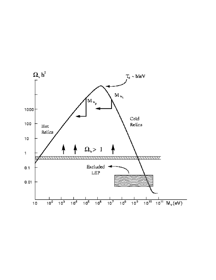
Figure 2: Plot of $\Omega_{\nu}h^{2}$ as a function of the neutrino (sum) mass.

VI.3 Accelerator limits and hints for neutrino masses

Two experiments at CERN, using $\nu_{\mu}$ beams of average neutrino energies $\langle E_{\nu_{\mu}}\rangle\sim 15~{}{\rm GeV}$ and typical decay lengths $L\sim 1~{}{\rm Km}$, put strong limits on $\nu_{\mu}\to\nu_{\tau}$ neutrino oscillations for $\Delta m^{2}\geq 10~{}{\rm eV}^{2}$. In view of the discussion in the last subsection, this is a very interesting mass range to explore, since neutrinos with masses in this range could be of cosmological interest.

These two experiments use quite different techniques to detect $\nu_{\tau}$’s. CHORUSchorus uses an emulsion target to try to detect the $\tau$ track produced in $\nu_{\tau}$ charged current interactions. NOMAD, nomad on the other hand, uses drift chambers and kinematical techniques to detect a $\nu_{\tau}$ signal. The result of both experiments are shown in Fig. 3, along with limits obtained by some earlier experiments. The CHORUS and NOMAD results for $\Delta m^{2}\geq 10~{}{\rm eV}^{2}$ exclude oscillations with mixing angles $\sin^{2}2\theta_{\mu\tau}\geq 10^{-3}$ at the 90% C.L., improving previous limits by about a factor of 5.

Because NOMAD has a very good electron identification, this experiment is also able to set a strong limit for $\nu_{\mu}\to\nu_{e}$ oscillations. For $\Delta m^{2}\geq 10~{}{\rm eV}^{2}$, one excludes oscillations with mixing angles $\sin^{2}2\theta_{\mu e}>2\times 10^{-3}$ at 90% C.L. Finally, because the $\nu_{\mu}$ beam at CERN has about a 1% $\nu_{e}$ admixture, both experiments are also able to exclude $\nu_{e}\to\nu_{\tau}$ oscillations for $\Delta m^{2}\geq 10~{}{\rm eV}^{2}$, but now only for mixing angles $\sin^{2}2\theta_{e\tau}\geq 10^{-1}$, at 90% C.L.

Figure 3: Bounds on $\nu_{\mu}\to\nu_{\tau}$ oscillations for large $\Delta m^{2}$, from [27].

The situation regarding neutrino oscillations is much less clear cut in the region $\Delta m^{2}\leq 10~{}{\rm eV}^{2}$. Here there are limits from past accelerator and reactor searches for oscillations and recent bounds from the KARMEN experiment. karmen . However, there is also some evidence for $\nu_{\mu}\to\nu_{e}$ oscillations coming from the LSND experiment.LSND Let me begin by briefly detailing the results of this last experiment first. LSND studies neutrinos originating from pions produced at rest at the LAMPF beam stop by an 800 MeV proton beam. These neutrinos, which are produced in the chain $\pi^{+}\to\mu^{+}\nu_{\mu}\to e^{+}\nu_{e}\bar{\nu}_{\mu}\nu_{\mu}$, have average momenta in the 30 to 50 MeV range. What LSND looks for is the oscillation of the $\bar{\nu}_{\mu}$ produced in $\mu^{+}$ decay into a $\bar{\nu}_{e}$, using a delayed coincidence in a target 30 meters from the beam dump. If $\bar{\nu}_{\mu}\to\bar{\nu}_{e}$ oscillations take place, the $\bar{\nu}_{e}$ inverse $\beta$-decay in the target ($\bar{\nu}_{e}p\to e^{+}n$) produces a prompt photon from $e^{+}e^{-}$ annihilation, while the produced neutron gives a delayed photon, as a result of the process $np\to d\gamma$.

The LSND experiment observes an excess of $e^{+}\gamma$ coincidence events which, if interpreted as $\bar{\nu}_{\mu}\to\bar{\nu}_{e}$ oscillations, give a substantial allowed region in the $\Delta m^{2}-\sin^{2}2\theta$ plane. However, as I mentioned above, other experiments performed in the past,past as well as the recent KARMEN experiment,karmen exclude almost all of this allowed region. Furthermore, new data from the KARMEN2 detectorK2 which became available in summer 1998 appeared to exclude even the small remaining allowed region for LSND!

This rather confusing situation is displayed in Fig. 4. It was discussed in some detail in the summary talk of Janet Conrad at the 1998 Vancouver International Conference on High Energy Physics.Conrad As one can see from Fig. 4, a combination of the BNL 776 data and the Bugey reactor data only leaves the region between $0.2~{}{\rm eV}^{2}<\Delta m^{2}<4~{}{\rm eV}^{2}$ as an “allowed” region for the LSND signal. However, this region is essentially excluded by the KARMEN2 data, if one uses the 90% C.L. bound from this experiment. However, this result itself is somewhat anomalous, since the 90% C.L. sensitivity for KARMEN2 is actually below the LSND signal. Furthermore, the LSND experiment has also looked for $\nu_{\mu}\to\nu_{e}$ oscillations by studying $\nu_{e}$ quasielastic scattering events and the collaboration, again, find an excess of events. citeLSND2 If interpreted as resulting from oscillations, this additional signal gives a $\Delta m^{2}-\sin^{2}2\theta$ allowed region which is consistent with that obtained by the $\bar{\nu}_{\mu}\to\bar{\nu}_{e}$ analysis.

It is difficult to make strong statements at this stage. The best that one can say is that there are hints of $\nu_{\mu}\to\nu_{e}$ oscillations in the region $0.2~{}{\rm eV}^{2}<\Delta m^{2}<4~{}{\rm eV}^{2}$, with rather small mixing angles $\sin^{2}2\theta_{\mu e}\sim 10^{-2}$.

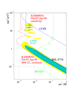
Figure 4: Summary of the experimental situation for $\bar{\nu}_{\mu}\to\bar{\nu}_{e}$ oscillations at the time of the Vancouver Conference, from Ref. [28].

VI.4 Atmospheric Neutrino Oscillations.

Large underground detectors, originally conceived to search for proton decay, are sensitive to the flux of neutrinos produced in the atmosphere. These neutrinos are mostly produced through the decay of pions, with the $\pi\to\mu\to e$ chain producing two $\nu_{\mu}$ neutrinos and antineutrinos for each $\nu_{e}$ neutrino and antineutrino. One has known since the early 1990’s that the observed flux of $\nu_{\mu}$’s appeared to be much smaller than expected, with the ratioratio

$$R=\frac{\left(\frac{\nu_{\mu}}{\nu_{e}}\right)_{\rm observed}}{\left(\frac{\nu_{\mu}}{\nu_{e}}\right)_{\rm expected}}\simeq 0.6~{}.$$ (145)

Although the anomalous ratio $R$ could be the result of neutrino oscillations, strong evidence for neutrino oscillations only emerged in summer 1998 from the SuperKamiokande experiment. The SuperKamiokande collaborationsuperK reported a pronounced zenith angle dependence for the flux of multi-GeV $\nu_{\mu}$ neutrinos, but no such dependence from $\nu_{e}$ neutrinos. For neutrino energies in the multi-GeV range, the neutrino fluxes are not affected by geomagnetic effects in an asymmetric fashion. Thus one expects the observed neutrino signal to be up-down symmetric. As can be seen in Fig. 5, the SuperKamiokande data for multi-GeV $\nu_{\mu}$’s is clearly up-down asymmetric. There are 139 up-going $\nu_{\mu}$ compared to 256 down going events. The observed asymmetry

$$\left(\frac{U-D}{U+D}\right)^{\rm Multi-GeV}_{\nu_{\mu}}=-0.296\pm 0.048\pm 0.010$$ (146)

is a $6\sigma$ effect. The corresponding asymmetry for multi-GeV $\nu_{e}$

$$\left(\frac{U-D}{U+D}\right)^{\rm Multi-GeV}_{\nu_{e}}=-0.036\pm 0.067\pm 0.020$$ (147)

is quite consistent with zero.

Figure 5: SuperKamiokande results on multi-GeV $\nu_{\mu}$ events.

The SuperKamiokande collaborationsuperK interprets these results as evidence for $\nu_{\mu}\to\nu_{X}$ oscillations, with $\nu_{X}$ some other neutrino species. This is most dramatically demonstrated in Fig. 6 where the ratio of data to Monte Carlo is plotted as a function of $L/E_{\nu}$ for both $\nu_{e}$ and $\nu_{\mu}$ events. No $L/E_{\nu}$ dependence is seen in the $\nu_{e}$ data, but the $\nu_{\mu}$ data drops down to a value of 1/2 for $L/E_{\nu}\geq 10^{3}~{}{\rm Km/GeV}$. Recalling the simple 2-neutrino formula for the probability of oscillations [Eq. (78)], Fig. 6 suggest immediately that $\Delta m^{2}\sim 10^{-3}~{}{\rm eV}^{2}$ and that the mixing angle $\theta$ is near maximal. This is confirmed by a more detailed analysis, which for $\nu_{\mu}\to\nu_{X}$ oscillations gives $\sin^{2}2\theta=1$ and $\Delta m^{2}=2.2\times 10^{-3}~{}{\rm eV}^{2}$ as the best fit point.

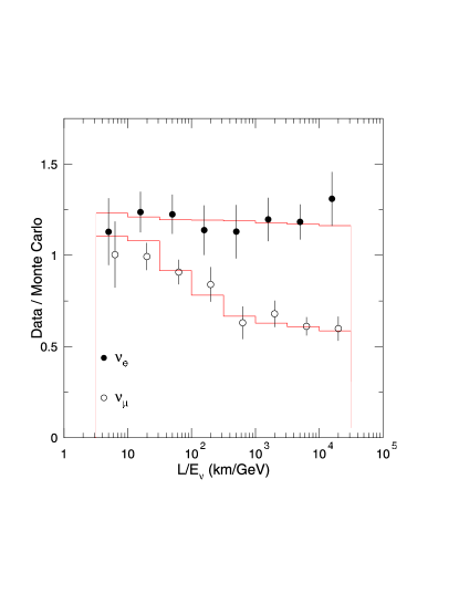
Figure 6: Plot of neutrino signals in the SuperKamiokande experiment as a function of $L/E_{\nu}$.

It is unlikely, however, that the SuperKamiokande results are due to $\nu_{\mu}\to\nu_{e}$ oscillations (that is, that $\nu_{X}\equiv\nu_{e}$). First, the region in the $\Delta m^{2}-\sin^{2}2\theta$ plane favored by the SuperKamiokande results, is almost totally excluded already by the null results of the CH00Z reactor experimentCH00Z which looks at $\nu_{e}$ oscillations into another neutrino species. Furthermore, the up-down ratio (129) for the $\nu_{e}$ flux is more than $3\sigma$ away from what one would expect if one were dealing with $\nu_{\mu}\to\nu_{e}$ oscillations, where one expects

$$\left(\frac{U-D}{U+D}\right)^{\rm theory}_{\nu_{\mu}\to\nu_{e}}=0.205~{}.$$ (148)

If there are only three neutrino species, then most likely what is being seen in SuperKamiokande are $\nu_{\mu}\to\nu_{\tau}$ oscillations. However, at this stage, it is not possible to rule out the possibility that $\nu_{X}$ may be a sterile neutrino $\nu_{s}$.

The SuperKamiokande resultssuperK are consistent with previous Kamiokande results,Kam which also had indicated a (less pronounced) zenith angle dependence of the $\nu_{\mu}$ flux. Although the $\Delta m^{2}-\sin^{2}2\theta$ regions for SuperKamiokande and Kamiokande do not appear to overlap much, the 90% C.L. region of SuperKamiokande is “more-significant”, since the Kamiokande best fit has $\sin^{2}2\theta=1.35$. In fact, recent results presented by SuperKamiokande at DPF 99,DPF99 with more data collected, help span the gap, indicating even more clearly the consistency of all data with each other.

In addition, data from other underground experiments (SoudanSoudan and MACROmacro ) as well as other phenomena—like the flux of upward going muons Kam2 produced by $\nu_{\mu}$ interactions in the earth—when interpreted in a neutrino oscillation framework, are totally consistent with the SuperKamiokande $\nu_{\mu}$ zenith angle results. Fig. 7 summarizes all this information in one graph. This figure provides quite strong evidence in favor of neutrino masses and is probably the strongest evidence we have to date for physics beyond the Standard Model.

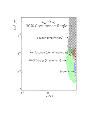
Figure 7: Evidence for atmospheric neutrino oscillations from all experiments, from Ref. [24].

VI.5 Solar Neutrinos

The study of the solar neutrino flux was started in the early 1970’s by Ray Davis and his group.Davis At present there are five different experiments which give information on solar neutrinos (Homestake,H Gallex,Gallex SAGE,Sage KamiokandeKamioka and SuperKamiokandeSuperK2 ) and all five have some bearing on the issue of neutrino oscillations. In fact, roughly speaking, all five experiments see approximately half of the expected rate, as shown in Fig. 8. However, these experiments are sensitive to different parts of the solar neutrino spectrum, because the reactions they use to detect solar neutrinos in their detectors have different thresholds. SAGE and Gallex study the reaction $\nu_{e}+{}^{71}{\rm Ga}\to{}^{71}{\rm Ge}+e^{-}$, which has a threshold of 0.23 MeV. Homestake looks for the excitation of chlorine ($\nu_{e}+{}^{37}{\rm Cl}\to{}^{37}{\rm Ar}+e^{-}$) which has a 0.8 MeV threshold. The water Cerenkov detectors, Kamiokande and SuperKamiokande, study elastic $\nu_{e}e$ scattering and their threshold is in the neighborhood of 6.5 MeV.

Figure 8: Rates seen by the diferent solar neutrino experiments, compared to the expectations of the Standard Solar Model. [49]

It has long been felt that the observed discrepancy between the neutrino signals detected and the expectations of the, so called, Standard Solar Model(SSM) BP is not due to defects in this model but to the presence of some new physical phenomena. One of the principal arguments in favor of this latter solution to the solar neutrino puzzle, has to do with the details of the signal expected in each experiment. Because of the quite different threshold involved, each of the solar neutrino experiments, in fact, feels different pieces of the neutrino producing reactions in the solar cycle. For example, the Gallium experiments are the only ones which are sensitive to neutrinos originating in the $pp$ cycle (the main solar cycle), with these neutrinos contributing about 50% of the expected rate. The Homestate detector mostly measures neutrinos from ${}^{8}B$, although it is also sensitive to ${}^{7}{\rm Be}$ neutrinos. Finally, because of their high threshold, the big water Cerenkov detectors only see Boron neutrinos. These circumstances make it difficult to argue for an astrophysical solution to the solar neutrino deficit. Much more natural is to imagine that this deficit arises as a result of neutrino oscillations.

There are two distinct neutrino oscillation solutions to the solar neutrino problem. Because roughly all experiments are reduced by about a factor of two from expectations, it is possible to fit the data by using vacuum neutrino oscillations $\nu_{e}\to\nu_{X}$. Clearly, for this fit one must appeal to large mixing angles and assume a tiny $\Delta m^{2}$. Since $E_{\nu}\sim{\rm MeV}$ and the earth-sun distance $L\sim 10^{11}~{}{\rm m}$, typically $\Delta m^{2}\sim 10^{-11}~{}{\rm eV}^{2}$. However, because the Homestake result is only about 30% of the predicted value, one has to fine-tune the parameters, so that only a few “just so” regions are favored. Barger A recent “just so” fit by Bahcall, Krastev, and SmirnovBKS is shown in Fig. 9.

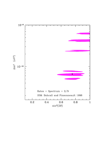
Figure 9: ”Just so” solar neutrino fit, from [51].

In my opinion, much more interesting that the above “solution” is the possibility that the solar neutrino results are a reflection of matter induced oscillations (the MSW effect we discuss in Section V). In the sun, the electron density to a good approximation, can be characterized by an exponential profile function Bah

$$N_{e}(r)=N_{e}(0)e^{-\frac{10r}{R_{0}}}~{}.$$ (149)

The central density $N_{e}(0)\simeq 10^{26}~{}{\rm cm}^{-3}\simeq 10^{12}~{}{\rm(eV)}^{3}$ is rather high and for appropriate values of $\Delta m^{2}$ and $\sin^{2}2\theta$ can exceed the critical MSW density. For instance, for $\theta$ small, $\Delta m^{2}\simeq 10^{-5}~{}{\rm eV}^{2}$ and $|p|\sim 3~{}{\rm MeV}$

$$N_{e}^{\rm crit}=\frac{\Delta m^{2}\cos^{2}\theta}{\sqrt{2}|p|G_{F}}\sim 10^{11}~{}{\rm(eV)}^{3}~{}.$$ (150)

It follows from Eq. (132) that, for these parameters, $\nu_{e}$’s produced in the core of the sum (where $N_{e}(o)\gg N_{e}^{\rm crit}$) as they radiate outward go through a region with $N_{e}\sim N_{e}^{\rm crit}$ and can oscillate to $\nu_{\mu}$’s (or other neutrino types) without paying a mixing angle penalty, since $\left.\sin 2\theta_{M}\right|_{N_{e}^{\rm crit}}\to 1$.

The actual calculation of what happens in the sun is rather complicated, Petcov since the density $N_{e}$ changes along the neutrino trajectory. Since $N_{e}=N_{e}(t)$, the matter Hamiltonian of Eq. (94) is now time dependent:

$$H_{\rm matter}(t)=\frac{\Delta m^{2}}{4|p|}\sin 2\theta\sigma_{1}-\left(\frac{\Delta m^{2}}{4|p|}\cos 2\theta-\frac{G_{F}}{\sqrt{2}}N_{e}(t)\right)\sigma_{3}~{}.$$ (151)

Although one can diagonalize this Hamiltonian, the resulting mixing angles and energies will be time dependent:

$$E_{1,2}^{M}(t)=\pm\left[\left(\frac{\Delta m^{2}}{4|p|}\cos 2\theta-\frac{G_{F}N_{e}(t)}{\sqrt{2}}\right)^{2}+\left(\frac{\Delta m^{2}}{4|p|}\sin 2\theta\right)^{2}\right]^{1/2}$$ (152)

$$\tan 2\theta_{M}(t)=\frac{\frac{\Delta m^{2}}{4|p|}\sin 2\theta}{\frac{\Delta m^{2}}{4|p|}\cos 2\theta-\frac{G_{F}N_{e}(t)}{\sqrt{2}}}~{}.$$ (153)

Because of this time dependence, it is no longer true that the states $|\nu_{1}^{M}(t)\rangle$ and $|\nu_{2}^{M}(t)\rangle$ are actual eigenstates. In fact, transitions can occur between these states. A simple calculation Petcov shows that the states $|\nu_{i}^{M}(t)\rangle$ obey a coupled Schrödinger equation

$$i\frac{\partial}{\partial t}\left[\begin{array}[]{c}|\nu_{1}^{M}(t)\rangle\\ |\nu_{2}^{M}(t)\rangle\end{array}\right]=\left[\begin{array}[]{cc}E_{1}^{M}(t)&i\frac{\partial}{\partial t}\theta_{M}(t)\\ i\frac{\partial}{\partial t}\theta_{M}(t)&E_{2}^{M}(t)\end{array}\right]\left[\begin{array}[]{c}|\nu_{1}^{M}(t)\rangle\\ |\nu_{2}^{M}(t)\rangle\end{array}\right]~{}.$$ (154)

If

$$|E_{2}^{M}(t)-E_{1}^{M}(t)|\gg\left|2\frac{\partial}{\partial t}\theta_{M}(t)\right|$$ (155)

then transiting between $|\nu_{1}^{M}(t)\rangle$ and $|\nu_{2}^{M}(t)\rangle$ will be relatively unimportant and one has an adiabatic situation. For an exponential density profile, Eq. (137) is satisfied at $N_{e}^{\rm crit}$ provided thatPetcov

$$\frac{\Delta m^{2}\sin^{2}2\theta}{2\cos 2\theta}\gg 2\times 10^{-8}~{}{\rm(eV)}^{2}~{}.$$ (156)

For the adiabatic case, one can use our discussion of matter oscillations to give a qualitative picture of how the MSW mechanism could work in the sun. Because at the solar core $N_{e}(o)\gg N_{e}^{\rm crit}$, according to Eq. (106) $|\nu_{e}\rangle\simeq|\nu_{2}^{M}(o)\rangle$. Because we are assuming adiabaticity, as the neutrinos diffuse out of the core of the sun, the state $|\nu_{2}^{M}(o)\rangle$ will evolve into $|\nu_{2}^{M}(t)\rangle$. That is, there are no transitions in the sun. Thus, when the neutrinos exit the sun, the state $|\nu_{2}^{M}(t_{\rm surface})\rangle$ will just simply become $|\nu_{2}\rangle$. Because

$$\langle\nu_{e}|\nu_{2}\rangle=\sin\theta~{},$$ (157)

it follows that, in this case,

$$P^{\rm adiabatic}_{\rm solar}(\nu_{e}\to\nu_{e};L)=\sin^{2}\theta~{}.$$ (158)

A more careful analysis shows that there are actually two MSW solutions, one adiabatic and one non-adiabatic,solarsol both having $\Delta m^{2}\sim 10^{-5}~{}{\rm eV}^{2}$. The adiabatic solution has large mixing angles $\sin^{2}2\theta\simeq 1$. Hence, according to Eq. (140), $P^{\rm adiabatic}_{\rm solar}(\nu_{e}\to\nu_{e};L)\simeq 1/2$ so, indeed, roughly half the flux is lost. The non-adiabatic solution has $\sin^{2}2\theta\sim 5\times 10^{-3}$. Furthermore, a rather large range in the $\Delta m^{2}-\sin^{2}2\theta$ plane is eliminated by the absence of a day/night effect, which would be a sign of matter oscillations in the earth. The favored MSW regions are depicted in Fig. 10.

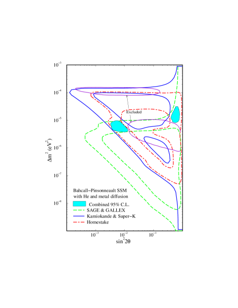
Figure 10: Regions in the the $\Delta m^{2}-\sin^{2}2\theta$ plane favored by the MSW explanations of the solar neutrino data, from Ref. [51].

I want to close this brief discussion of solar neutrinos, and in particular of the MSW explanation of the solar data, by making a more quantitative remark. To fit the solar neutrino data using the MSW effect requires that the probability $P(\nu_{e}\to\nu_{e};L)$ have considerable energy dependence. The required energy dependence is shown in Fig. 11. I indicate also in this figure at what energies the neutrinos produced in the various solar reactions are effective. One sees from Fig. 11 that essentially all $pp$ neutrinos survive, the Berylium neutrinos disappear and the flux of Boron neutrinos is roughly halved. This reconciles nicely with what is seen in the data, as detailed in Table 3.

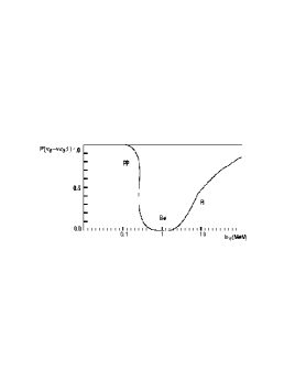
Figure 11: Energy dependence needed for $P(\nu_{e}\to\nu_{e};L)$ to fit the solar neutrino data.[54]

Table 3.  Summary of neutrino flux observations and expectations of solar

neutrino experiments

${}^{37}{\rm Cl}~{}(13\%~{}{\rm Be};~{}80\%~{}{\rm B})$
$(2.56\pm 0.23)~{}{\rm SNU}~{}{\rm Ref.}[44]~{}~{}~{}\left[\mbox{predicted SSM}:~{}\left(7.7^{+1.2}_{-1.0}\right)~{}{\rm SNU}\right]$

${}^{71}{\rm Ga}~{}(51\%~{}{\rm pp};~{}15\%~{}{\rm Be};~{}12\%~{}{\rm B})$
$(77.5\pm 7.7)~{}{\rm SNU}~{}{\rm Ref.}[45]~{}~{}~{}[\mbox{predicted SSM}:~{}(129\pm 8)~{}{\rm SNU}]$
$(66.6\pm 8.0)~{}{\rm SNU}~{}{\rm Ref.}[46]$

${\rm Water}~{}\check{C}~{}(100\%~{}{\rm B})$
$2.80\pm 0.38~{}{\rm SNU}~{}{\rm Ref}.[47]~{}~{}~{}[\mbox{predicted SSM}:~{}\left(5.15^{+1.0}_{-0.7}\right)~{}{\rm SNU}]$
$2.44\pm 0.10~{}{\rm SNU}~{}{\rm Ref.}[48]$

VII Theoretical Implications

I summarize in Fig. 12 where one is at present on the issue of neutrino masses and mixings. This figure collects together all the neutrino oscillation evidence, as well as the hints for oscillations, which we have at the moment. As is clear from the figure there are three regions suggested in the $\Delta m^{2}-\sin^{2}2\theta$ plane. The strongest evidence is that for atmospheric neutrino oscillations coming from the SuperKamiokande zenith angle data. Here the suggested parameters are $(\Delta m^{2})\sim 3\times 10^{-3}~{}{\rm eV}^{2}$, $\sin^{2}2\theta\sim 1$ with $\nu_{\mu}\to\nu_{X}~{}(\nu_{X}\not=\nu_{e})$. Solar neutrinos also are strongly suggestive of oscillations. Interpreting the data this way leads to $(\Delta m^{2})\sim 10^{-5}~{}{\rm eV}^{2}$, with $\sin^{2}2\theta\sim 1$ or $\sin^{2}2\theta\sim 5\times 10^{-3}$, for MSW $\nu_{e}\to\nu_{X}$ oscillations, or $\Delta m^{2}\sim 10^{-11}~{}{\rm eV}^{2}$ and $\sin^{2}2\theta\sim 1$, for “just-so” $\nu_{e}\to\nu_{X}$ oscillations. The weakest hint for oscillations probably is that of LSND, because of other contrary evidence. At any rate, the suggested region here is $\Delta m^{2}\sim 5\times 10^{-1}~{}{\rm eV}^{2}$ and $\sin^{2}2\theta\sim 10^{-2}$ for $\nu_{e}\to\nu_{\mu}$ oscillations.

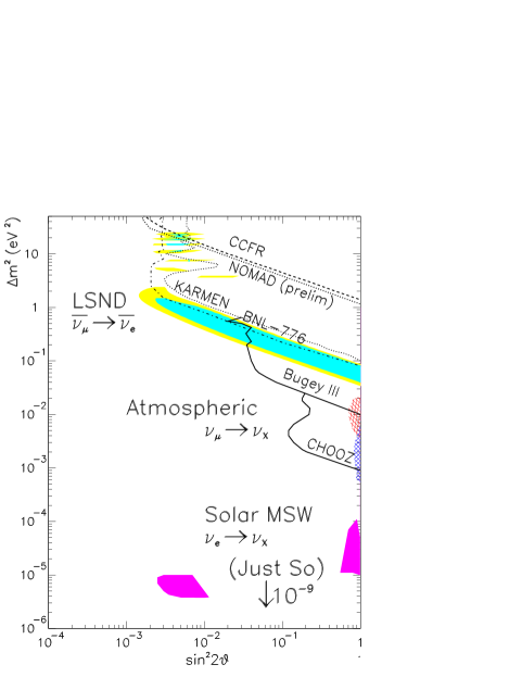
Figure 12: Summary of evidence of, and hints for, neutrino oscillations.[24]

Besides neutrino oscillation phenomena, there is really no other direct evidence for neutrino masses. However, both $\beta$-decay and neutrinoless double $\beta$-decay put rather strong bounds on neutrino masses connected to $\nu_{e}$. From $\beta$-decay the largest neutrino mass obeys the bound: “$m_{\nu_{e}}$” $<3.9~{}{\rm eV}$ (90% C.L.). Double $\beta$-decay, bounds the Majorana mass $\langle m_{\nu_{e}}\rangle_{ee}$ even more strongly: $\langle m_{\nu_{e}}\rangle_{ee}<0.2~{}{\rm eV}$ (90% C.L.). These bounds are interesting, since they are close to the kind of neutrino masses which could have substantial cosmological influence. Using the central value for the Hubble parameter [c.f. Eq.(124)], I note that $\sum_{i}m_{\nu_{i}}=30~{}{\rm eV}$, 6 eV, 2 eV correspond, respectively, to neutrinos closing the Universe, to neutrinos being 20% of the dark matter in the Universe (assuming $\Omega_{M}\simeq 1$), and to neutrinos being 20% of the dark matter, with $\Omega_{M}\simeq 0.3$. The last case is, perhaps, the one that is most cosmologically realistic. cosmo This stresses the the importance of continuing the search for neutrino masses in the eV range.

Concentrating only on the SuperKamiokande evidence for neutrino masses already has important implications. Taking

$$\Delta m^{2}=m_{3}^{2}-m_{2}^{2}\sim 3\times 10^{-3}~{}{\rm eV}^{2}$$ (159)

gives one already a lower bound on some neutrino mass: $m_{3}\geq 5\times 10^{-2}~{}{\rm eV}$. This mass value, in turn, gives a lower bound for the cosmological contribution of neutrinos

$$\Omega_{\nu}\geq\frac{m_{3}}{92~{}{\rm eV}~{}h^{2}}\sim 1.5\times 10^{-3}~{}.$$ (160)

Although this number is far from that needed for closure of the Universe, I note that the $\Omega_{\nu}$ of Eq. (142) is comparable to the contribution of luminous matter to the energy density of the Universeluminous

$$\Omega_{\rm luminous}\sim(3-7)\times 10^{-3}~{}.$$ (161)

So, from SuperKamiokande we learn that the neutrino contribution to the energy density of the Universe is the same as, in the words of Carl Sagan, that of “billions and billions of stars”!

For particle physics, a value of $m_{3}\sim 5\times 10^{-2}~{}{\rm eV}$ is also quite interesting. If we use either the simple see-saw formula of Eq. (55) or the GUT relation (66), the identification

$$m_{3}=\left\{\begin{array}[]{l}\frac{[(m_{D})_{3}]^{2}}{m_{S}}\sim\frac{m_{t}^{2}}{m_{S}}\\ m_{T}\simeq\frac{\langle\phi^{0}\rangle^{2}}{\Lambda}\end{array}\right.$$ (162)

give comparable values for $m_{S}$ and $\Lambda$:

$$m_{S}\sim\Lambda\sim 10^{15}~{}{\rm GeV}~{}.$$ (163)

Of course, these values are only justifiable in specific models where one has a bit more control of other constants, which are taken above all to be of $O(1)$.

If one goes beyond the SuperKamiokande data, then many theoretical scenarios emerge. Unfortunately, in general, these scenarios mostly reflect the prejudices one has regarding the data. Nevertheless, it is useful to briefly discuss two differing broad theory scenario. In the first scenario, one assumes that all hints for oscillations seen are true. In the second, one disregards some oscillation hints. In most cases, the discarded data is that of LSND.

If one believes all hints for neutrino oscillations, since there are three different $\Delta m^{2}$ involved, the neutrino mass matrix $M$ necessarily is a $4\times 4$ matrix. To get a $4\times 4$ neutrino matrix one adds to the usual three neutrinos a sterile neutrino $\nu_{s}$. Most 4 neutrino models attempt to fit all data, since this was after all the reason for introducing the fourth neutrino. The most promising scenariofitall has two pairs of quasi-Dirac neutrinos split by a small mass difference. The heaviest pair ($m_{2}$ and $m_{3}$) have masses of order 0.5 eV and contribute $\Omega_{\nu}\simeq 0.03$ to cosmology. The atmospheric neutrino oscillations involve this pair, so that $\Delta m^{2}_{23}\sim 3\times 10^{-3}~{}{\rm eV}^{2}$. The second pair ($m_{1}$ and $m_{4}$) are much lighter, with mass around $10^{-2}-10^{-1}~{}{\rm eV}$. Their mass difference $\Delta m^{2}_{14}\sim 10^{-5}~{}{\rm eV}^{2}$ is what enters in solar neutrino oscillations. The LSND result is explained as an oscillation between the light pair and the heavy pair, with $\Delta m^{2}\sim m^{2}_{3}\sim 0.6~{}{\rm eV}^{2}$. In this scheme, the solar neutrino oscillations involve oscillations of $\nu_{e}$ to a sterile neutrino, while the atmospheric neutrino oscillation is $\nu_{\mu}\to\nu_{\tau}$ and LSND $\nu_{e}\to\nu_{\mu}$. Although this scheme works phenomenologically, theoretically it is difficult to get light sterile neutrinos almost degenerate with ordinary neutrinos.

Different patterns arise if one is prepared to disregard some of the neutrino oscillation limits. If one disregards, in particular, the results from LSND then the CH00Z bound,CH00Z and the quite different mass squared differences involved in atmospheric and solar neutrino oscillations, suggest a very simple 3-neutrino mixing matrix. CH00Z suggests that $\theta_{13}\simeq 0^{o}$. On the other hand, atmospheric neutrino oscillations suggest $\theta_{23}\simeq 45^{o}$. Finally, depending on what solar neutrino oscillation solution one picks, the angle $\theta_{12}$ can either be large or small. Thus, neglecting possible CP violating phases, the neutrino mixing matrix looks likeAlta

$$U \simeq\left[\begin{array}[]{ccc}1&0&0\\ 0&\frac{1}{\sqrt{2}}&-\frac{1}{\sqrt{2}}\\ 0&\frac{1}{\sqrt{2}}&\frac{1}{\sqrt{2}}\end{array}\right]\left[\begin{array}[]{ccc}1&0&0\\ 0&1&0\\ 0&0&1\end{array}\right]\left[\begin{array}[]{ccc}c_{12}&-s_{12}&0\\ s_{12}&c_{12}&0\\ 0&0&1\end{array}\right]$$ (173)

$$=\left[\begin{array}[]{ccc}c_{12}&-s_{12}&0\\ \frac{s_{12}}{\sqrt{2}}&\frac{c_{12}}{\sqrt{2}}&-\frac{1}{\sqrt{2}}\\ \frac{s_{12}}{\sqrt{2}}&\frac{c_{12}}{\sqrt{2}}&\frac{1}{\sqrt{2}}\end{array}\right]~{},$$ (177)

where $c_{12}=\cos\theta_{12};~{}s_{12}=\sin\theta_{12}$. However, even with $U$ of the above form, there are many open questions to answer. For instance, is maximal mixing $(\theta_{12}\simeq 45^{o})$ allowed? Are nearly degenerate neutrino masses $(m_{1}\simeq m_{2}\simeq m_{3}\simeq 0.5~{}{\rm eV})$ allowed? What neutrino mass matrix gives rise to this particular mixing matrix?

These questions cannot really be answered in a straightforwad manner, without making some more assumptions. There is really a lot of freedom. Given $U$ and some assumptions for the neutrino mass spectrum $\{m_{i}\}$ then one can deduce a neutrino mass matrix $M$. However, recall from our discussion of the see-saw mechanism, that $M$ itself depends on both the neutrino Dirac mass $m_{D}$ and on the right-handed neutrino mass matrix $m_{S}$ [cf. Eq. (55)]. Thus, to make progress, even “knowing” $M$ one has to make some assumptions on $m_{D}$ (or $m_{S}$) to learn something further. For instance, one could use GUTs which naturally ties the matrix $m_{D}$ in Eq. (55) to the $u$-quark mass matrix. Babu

Some authors have preferred to focus on some simple structure for the $3\times 3$ matrix $M$. Barbieri Two of these are particularly appealing. The first of these has a total degeneracy for the neutrinos, the other is Dirac-like with an additional massless neutrino. In the first pattern

$$M=m\left(\begin{array}[]{ccc}1&0&0\\ 0&0&1\\ 0&1&0\end{array}\right)~{}.$$ (178)

In this case, $\sum_{i}m_{\nu_{i}}=3m$, so that cosmology impose a bound on $m$, depending on what one believes $\Omega_{\nu}$ is. However, in the degenerate case, one has also that

$$\langle m_{\nu_{e}}\rangle_{ee}=\sum_{i}U^{2}_{ei}m_{\nu_{i}}=m~{}.$$ (179)

The double $\beta$-decay bound then tell us that $m<0.2$ eV. If we push $m$ to its upper bound, however, it is difficult to see what perturbation can then give $\Delta m^{2}_{\rm atmos}\simeq 3\times 10^{-3}~{}{\rm eV}^{2};~{}\Delta m^{2}_{\rm solar}\sim 10^{-5}~{}{\rm eV}^{2}$.

The second simple pattern for neutrino masses has Hall

$$M=m\left(\begin{array}[]{ccc}0&1&1\\ 1&0&0\\ 1&0&0\end{array}\right)$$ (180)

which has a degenerate pair and a zero eigenvalue. Note that this pattern conserves $L_{e}-L_{\mu}-L_{\tau}$. Since for this mass matrix $\Delta m^{2}_{\rm atmos}=m^{2}$, it follows that $m\sim 5\times 10^{-2}~{}{\rm eV}$. So in this case, neutrinos do not contribute much to the energy density of the Universe $(\Omega_{\nu}\simeq 3\times 10^{-3})$. To get solar neutrino oscillations one has to introduce some perturbation on the mass matrix (149) that will split the massive degenerate states and give $\Delta m^{2}_{12}\sim 10^{-5}~{}{\rm eV}^{2}$.

VIII Future Experiments

It seems pretty clear that progress in understanding what is going on in the neutrino sector can only come from further data. Fortunately, new data will be forthcoming in all the relevant $\Delta m^{2}$ regions. I want to end these lectures by briefly discussing these future experiments.

VIII.1 Solar Neutrinos

SuperKamiokande will continue to take data in years to come, thus refining their present measurements of solar neutrinos. Furthermore, a real effort is taking place to lower the neutrino energy threshold further so as to be able to study the shape dependence of the signal as a function of $E_{\nu}$. In addition to this continuing effort, relatively soon two other experiments will be coming on line which have considerable promise. The first of these is SNO (the Sudbury Neutrino Observatory SNO ) which uses a Kiloton of D₂O. The advantage of having heavy water is that it allows SNO to study simultaneously both charged current and neutral current processes. The charged current process

$$\nu_{e}+d\to e^{-}+p+p~{},$$ (181)

like all charged current processes, is sensitive to whether oscillations have occurred or not. The neutral current disintegration of the deuteron, on the other hand, is insensitive to oscillations since it is the same for all neutrino species $\nu_{X}$:

$$\nu_{X}+d\to\nu_{X}+p+n~{}.$$ (182)

Comparison of the rates for the two neutrino reactions(150) and (151) should help rule out possible astrophysical explanations for the solar neutrino puzzle. The SNO detector should begin taking data in 1999.

The second solar neutrino experiment of interest is Borexino. Borexino This experiment is presently under construction at the Gran Sasso Laboratory and should be ready for data taking in 2001. Borexino uses 300 tons of scintillator, which has a relatively low threshold $(E_{\rm thr}>340~{}{\rm KeV})$. As a result, Borexino should be particularly sensitive to the $E_{\nu}=862~{}{\rm GeV}$ neutrino line coming from ⁷Be. Recalling Fig. 11, one sees that if the MSW explanation is correct, the solar neutrino signal in Borexino should be significantly below the theoretical expectations. Indeed, if there are no solar oscillations, Borexino is supposed to detect about 50 events/day, while if the MSW explanation is true, this number should go down to about 10 events/day.

VIII.2 Atmospheric Neutrinos

Here again SuperKamiokande will continue to integrate data with time. However, the $\Delta m^{2}$ region, will also be probed more directly by using neutrino beams from accelerators. Three such long baseline experiments are in different stages of readiness. K2K, which uses a neutrino beam from KEK, aimed at SuperKamiokande 250 Km away, should shortly be operational. K2K MINOS,MINOS in the Soudan Mine, is under construction and will be the target of a dedicated neutrino beam from Fermilab, 730 Km away. First data should become available around 2001-2002. Finally, a variety of proposals exist for experiments in the Gran Sasso Laboratory, which is 740 Km from CERN, to become targets of neutrino beams from CERN.

The main advantage that these long baseline experiments have over SuperKamiokande is that the neutrino beam used is well characterized, both in energy and in its time structure. Furthermore, these beams also have a higher intensity. So many possible systematic effects will be under better control. In the case of the higher energy Fermilab and CERN beams, it may also be possible to directly search and detect $\nu_{\tau}$’s, if these neutrinos are produced in the oscillations.

VIII.3 LSND Region

The $\Delta m^{2}-\sin^{2}2\theta$ region identified by the LSND experiment as potentially interesting also will be explored further. At Fermilab, there is an approved experiment, Mini BooNE, Boone which will run around 2001-2002, which should be about a factor of five more sensitive than LSND in a comparable kinematical region. With this sensitivity, it should be quite clear whether $\nu_{\mu}\to\nu_{e}$ oscillations with $\Delta m^{2}\sim(0.1-1)~{}{\rm eV}^{2}$ exist or not.

Appendix A: Dirac and Majorana Masses

To understand how Dirac and Majorana masses can arise, it is useful to review here some of the properties of the spinor representations of the Lorentz group. The Lorentz group, besides the well known vector and tensor representations has also spinor representations. It turns out that there are two inequivalent spinor representations. It is out of these two-dimensional spinors that one builds up the usual four-dimensional Dirac spinor $\psi$.

Under a Lorentz transformation, a vector field $V^{\mu}$ has the well known transformation

$$V^{\mu}\to V^{\prime\mu}=\Lambda^{\mu}_{~{}\nu}V^{\nu}~{},$$ (1)

where the 4-dimensional representation matrices $\Lambda$ obey the pseudo-orthogonality conditions

$$\eta_{\mu\nu}=\Lambda^{\alpha}_{~{}\mu}\eta_{\alpha\beta}\Lambda^{\beta}_{~{}\nu}~{},$$ (2)

involving the metric tensor

$$\eta_{\mu\nu}=\left[\begin{array}[]{cccc}-1&&&\\ &1&&\\ &&1&\\ &&&1\end{array}\right]~{}.$$ (3)

Besides vector representations, the Lorentz group has two inequivalent spinor representation. The corresponding 2-dimensional Weyl spinors are conventionally denoted by $\xi_{a}$ and $\dot{\xi}_{a}$, known as undotted and dotted spinors, respectively. Under Lorentz transformations they transform as

$$\xi_{a}\to\xi_{a}^{\prime} = M_{a}^{~{}b}\xi_{b}$$ (4)

$$\dot{\xi}_{a}\to\dot{\xi}_{a}^{\prime} = M_{a}^{*b}\dot{\xi}_{b}~{}.$$ (5)

The $2\times 2$ matrices $M$ and $M^{*}$, with det $M={\rm det}~{}M^{*}=1$, provide inequivalent representation of $SL(2,C)$. Obviously, from the above it follows that $\dot{\xi}\sim\xi^{*}$.

One can establish a relationship between the $2\times 2$ matrices $M$ and the $4\times 4$ matrices $\Lambda$, since the vector field $V^{\mu}$ transforms as $V\sim\xi\otimes\dot{\xi}$. For these purposes, it is useful to define a set of four matrices $\sigma^{\mu}\equiv(1,\vec{\sigma})$, with $\vec{\sigma}$ being the usual Pauli matrices. The $2\times 2$ matrix

$$V=\sigma^{\mu}\eta_{\mu\nu}V^{\nu}\equiv\sigma^{\mu}V_{\mu}$$ (6)

under a Lorentz transformation transforms as

$$V\to V^{\prime}=MVM^{\dagger}=\sigma^{\mu}V_{\mu}^{\prime}~{}.$$ (7)

Using Eq. (A1), it follows that

$$\sigma^{\mu}_{ac}\Lambda_{\mu}^{~{}\nu}=M_{a}^{~{}b}\sigma_{bd}^{\nu}M_{c}^{*d}~{}.$$ (8)

Because det $M=1$, the analogue of the scalar product for vectors $V^{\mu}\eta_{\mu\nu}V^{\nu}\equiv V^{\mu}V_{\mu}$, for the spinors $\xi$ and $\dot{\xi}$ leads to the following Lorentz scalars:

$$\xi_{a}\epsilon^{ab}\xi_{b}\equiv\xi_{a}\xi^{b}~{};~{}~{}~{}~{}~{}\dot{\xi}_{a}\epsilon^{ab}\dot{\xi}_{b}\equiv\dot{\xi}_{a}\dot{\xi}^{b}$$ (9)

where $\epsilon^{ab}=-\epsilon^{ba}$ and $\epsilon^{12}=1$. Similarly, just as the contraction of a covariant and contravariant metric tensor gives the identity $[\eta_{\mu\rho}\eta^{\rho\nu}=\delta_{\mu}^{\nu}]$, one can define $2\times 2$ antisymmetric $\epsilon$-matrices, $\epsilon_{ab}$, which obey

$$\epsilon_{ac}\epsilon^{cb}=\delta_{a}^{b}~{}.$$ (10)

It follows that $\epsilon_{12}=-1$.

The usual 4-component Dirac spinor $\psi$ is made up of a dotted and an undotted Weyl spinor:

$$\psi=\left(\begin{array}[]{c}\xi_{a}\\ \dot{\chi}^{a}\end{array}\right)$$ (11)

In this, so called, Weyl-basis the Dirac $\gamma$-matrices $\gamma^{\mu}$, which obey the anticommutation relations $\{\gamma^{\mu},\gamma^{\nu}\}=-2\eta^{\mu\nu}$, take the form

$$\gamma^{\mu}=\left(\begin{array}[]{cc}0&\sigma^{\mu}\\ \bar{\sigma}^{\mu}&0\end{array}\right)~{}.$$ (12)

Here $\bar{\sigma}^{\mu}=(1,-\vec{\sigma})$, so that in this basis

$$\gamma^{0}=\left(\begin{array}[]{cc}0&1\\ 1&0\end{array}\right)~{};~{}~{}~{}~{}~{}\gamma^{i}=\left(\begin{array}[]{cc}0&\sigma^{i}\\ -\sigma^{i}&0\end{array}\right)$$ (13)

and

$$\gamma_{5}=i\gamma^{0}\gamma^{1}\gamma^{2}\gamma^{3}=\left(\begin{array}[]{cc}-1&0\\ 0&1\end{array}\right)~{}.$$ (14)

It follows from the above that $\xi_{a}$ and $\dot{\chi}^{a}$ are chiral projections of $\psi$:

$$\psi_{\rm L}=\frac{1}{2}(1-\gamma_{5})\psi = \left(\begin{array}[]{c}\xi_{a}\\ 0\end{array}\right)~{};~{}~{}~{}~{}\overline{\psi_{\rm L}}=\bar{\psi}\frac{1}{2}(1+\gamma_{5})=(0~{}~{}\xi^{*}_{a})$$ (17)

$$\psi_{\rm R}=\frac{1}{2}(1+\gamma_{5})\psi = \left(\begin{array}[]{c}0\\ \dot{\chi}^{a}\end{array}\right)~{};~{}~{}~{}~{}\overline{\psi_{\rm R}}=\bar{\psi}\frac{1}{2}(1-\gamma_{5})=(\dot{\chi}^{a*}~{}0)~{}.$$ (20)

Using these equations, it is easy to see that the Dirac mass term connects $\xi$ with $\dot{\chi}$. Specifically, one has

$${\cal{L}}_{\rm Dirac}=-m_{D}(\overline{\psi_{\rm L}}\psi_{\rm R}+\overline{\psi_{\rm R}}\psi_{\rm L})=-m_{D}(\xi^{*}_{a}\dot{\chi}^{a}+\dot{\chi}^{a*}\xi_{a})~{}.$$ (21)

Recall, however, that dotted spinors are related to the complex conjugate of an undotted spinor. Choosing a phase convention where

$$\xi^{*}_{a}=\dot{\xi}_{a}~{};~{}~{}~{}~{}\dot{\chi}_{a}^{*}=\chi_{a},$$ (22)

one can write the Dirac mass term simply as

$${\cal{L}}_{\rm Dirac}=-m_{D}(\dot{\xi}_{a}\dot{\chi}^{a}+\chi^{a}\xi_{a})~{}.$$ (23)

In view of Eq. (A9) this term is obviously Lorentz invariant. However, Lorentz invariance does not require one to have two distinct Weyl spinors $\xi$ and $\chi$ to construct a mass term. Majorana masses, basically, make use of this “simpler” option.

One can define a 4-component Majorana spinor in terms of the Weyl spinor $\xi$ and its complex conjugate $\dot{\xi}$:

$$\psi_{M}=\left(\begin{array}[]{c}\xi_{a}\\ \dot{\xi}^{a}\end{array}\right)~{}.$$ (24)

Because $\dot{\xi}^{a}=\xi^{a*}$, effectively $\psi_{M}$ has only one independent helicity projection. One can choose this projection to be, say, $(\psi_{M})_{\rm L}$:

$$(\psi_{M})_{\rm L}=\frac{1}{2}(1-\gamma_{5})\psi_{M}=\left(\begin{array}[]{c}\xi_{a}\\ 0\end{array}\right)~{};~{}~{}~{}~{}{\overline{(\psi_{M})_{\rm L}}}=\overline{\psi_{M}}\frac{1}{2}(1+\gamma_{5})=(0~{}~{}\dot{\xi}_{a})~{}.$$ (25)

One can construct $(\psi_{M})_{\rm R}$ by using the charge conjugate matrix $\tilde{C}$. In the Weyl basis $\tilde{C}$ is given by

$$\tilde{C}=\left[\begin{array}[]{cc}\epsilon_{ab}&0\\ 0&\epsilon^{ab}\end{array}\right]=\left[\begin{array}[]{cccc}0&-1&0&0\\ 1&0&0&0\\ 0&0&0&1\\ 0&0&-1&0\end{array}\right]~{}.$$ (26)

Clearly

$$(\psi_{M})_{\rm R} = \left(\begin{array}[]{c}0\\ \dot{\xi}^{a}\end{array}\right)=\left(\begin{array}[]{c}0\\ \epsilon^{ab}\dot{\xi}_{b}\end{array}\right)=\tilde{C}{\overline{(\psi_{M})_{\rm L}}}^{T}$$ (31)

$$\overline{(\psi_{M})_{\rm R}} = (\xi^{a}~{}0)=(\epsilon^{ab}\xi_{b}~{}0)=(\xi_{b}\epsilon_{ba}~{}0)=(\psi_{M})^{T}_{\rm L}\tilde{C}~{}.$$ (32)

That is, $(\psi_{M})_{\rm R}$ is the charge conjugate of $(\psi_{M})_{\rm L}$ (c.f. Eq. (36)):

$$[(\psi_{M})_{\rm L}]^{c}=(\psi_{M})_{\rm R}~{}.$$ (33)

Because of Eq. (A24) it follows that the Majorana spinor $\psi_{M}$ obeys a constraint. It is self-conjugate:

$$\psi_{M}=\left(\begin{array}[]{c}\xi_{a}\\ \dot{\xi}^{a}\end{array}\right)=(\psi_{M})_{\rm L}+(\psi_{M})_{\rm R}=(\psi_{M})_{\rm L}+[(\psi_{M})_{\rm L}]^{c}~{}.$$ (34)

Hence,

$$\psi_{M}=[\psi_{M}]^{c}~{}.$$ (35)

The Majorana mass term

$${\cal{L}}_{\rm Majorana}=-\frac{1}{2}m_{M}\overline{\psi_{M}}\psi_{M}$$ (36)

involves a product of $\xi$ with itself and $\dot{\xi}$ with itself

$${\cal{L}}_{\rm Majorana}=-\frac{1}{2}m_{M}\left({\overline{(\psi_{M})_{\rm L}}}(\psi_{M})_{\rm R}+{\overline{(\psi_{M})_{\rm R}}}(\psi_{M})_{\rm L}\right)=-\frac{1}{2}m_{M}(\dot{\xi}_{a}\dot{\xi}^{a}+\xi^{a}\xi_{a})~{}.$$ (37)

Eq. (A28) can also be written purely in terms of $(\psi_{M})_{\rm L}$ by using the charge conjugation matrix $\tilde{C}$. Using Eq. (A23) one has also

$${\cal{L}}_{\rm Majorana}=-\frac{1}{2}m_{M}\left({\overline{(\psi_{M})_{\rm L}}}\tilde{C}{\overline{(\psi_{M})_{\rm L}}}~{}^{T}+(\psi_{M})_{\rm L}^{T}\tilde{C}(\psi_{M})_{\rm L}\right)~{}.$$ (38)

Equally well one can write this mass term entirely as a function of $(\psi_{M})_{\rm R}$. One finds

$${\cal{L}}_{\rm Majorana}=-\frac{1}{2}\left((\psi_{M})_{\rm R}^{T}\tilde{C}(\psi_{M})_{\rm R}+{\overline{(\psi_{M})_{\rm R}}}\tilde{C}{\overline{(\psi_{M})_{\rm R}}}~{}^{T}\right)~{}.$$ (39)

References

- (1) A compilation of the latest electroweak data from LEP and the SLC is in the report of the LEP Electroweak Working Group, CERN-EP/99-15, February 1999.
- (2) Particle Data Group, C. Caso et al., Europ. Phys. J. C3 (1998) 1.
- (3) For a discussion, see for example, F. A. Berends et al., in Z Physics at LEP 1, eds. G. Altarelli, R. Kleiss and C. Verzegnassi, Vol 1, p. 89, CERN report CERN 89-08, 1989.
- (4) See, for example, R. D. Peccei, in Broken Symmetries, eds. L. Mathelitsch and W. Plessas, Lecture Notes in Physics 521 (Springer Verlag, Berlin 1999).
- (5) See, for example, J. D. Bjorken and S. D. Drell, Relativistic Quantum Fields (Mc Graw Hill, New York 1965).
- (6) T. Yanagida, in Proceedings of the Workshop on the Unified Theories and Baryon Number in the Universe, Tsukuba, Japan 1979, eds. O. Sawada and A. Sugamoto, KEK Report No. 79-18; M. Gell-Mann, P. Ramond and R. Slansky in Supergravity, Proceedings of the Workshop at Stony Brook, NY, 1979, eds. P. van Nieuwenhuizen and D. Freedman (North-Holland, Amsterdam, 1979).
- (7) G. Gelmini and M. Roncadelli, Phys. Lett. 99B (1981) 411.
- (8) See, for example, A. Masiero, R. N. Mohapatra and R. D. Peccei, Nucl. Phys. B192 (1981) 66.
- (9) See, for example, S. Weinberg, in Proceedings of the XXIII International Conference on High Energy Physics, Berkeley, California 1986, ed. S. C. Loken (World Scientific, Singapore 1987).
- (10) Some recent reviews which discuss this material include, W. C. Haxton and B. R. Holstein, to appear in the American Journal of Physics, hep-ph/9905257; P. Fisher, B. Kayser and K. S. McFarland, to appear in the Annual Review of Nuclear and Particle Science, Vol. 49 (1999), hep-ph/9906244
- (11) S. P. Mikheyev and A. Y. Smirnov, Sov. J. Nucl. Phys. 42 (1985) 441; Nuovo Cimento 9C (1986) 17; L. Wolfenstein, Phys. Rev. D17 (1978) 2369.
- (12) See, for example, S. T. Petcov, in Computing Particle Properties, eds. H. Gausterer and C. Lang, Lecture Notes in Physics 512 (Springer Verlag, Berlin 1998).
- (13) For early work on neutrino mass limits, see for example, D. R. Hamilton, W. P. Alford and L. Gross, Phys. Rev. 92 (1953) 1521.
- (14) For a recent review see, for example, K. Zuber, Phys. Rept. 305 (1998) 295.
- (15) V. Lobashev, to be published in the Proceedings of the 17th International Workshop on Weak Interactions and Neutrinos WIN 99, Capetown, South Africa, January 1999; see also, V. Lobashev, Prog. Part. Nucl. Phys. 40 (1998) 337; for earlier results see, A.I. Belesev et al. , Phys. Lett. B350 (1995) 263.
- (16) K. Assamagan et al. Phys. Rev. D53 (1996) 6065.
- (17) ALEPH Collaboration, R. Barate et al., Europ. Phys. J. C2 (1998) 395.
- (18) The first laboratory meausurement of double -decay in 82Se is reported in S. R. Elliot, A.A. Hahn and M. Moe, Phys. Rev. Lett. 59 (1987) 1649.
- (19) For a recent review see, for example, A. Morales in the Proceedings of the 18th International Conference on Neutrino Physics and Astrophysics, Tokayama, Japan, June 1998.
- (20) Heidelberg- Moscow Collaboration, L. Baudis et al. hep-ex/9902014.
- (21) For a discussion see, P. Vogel and M. Moe, Ann. Rev. Nucl. Part. Phys. 44 (1994) 247. For a recent review see, A. Faessler and F. Simkovic, hep-ph/9901215.
- (22) See, for example, E. W. Kolb and M. Turner, The Early Universe (Addison-Wesley, Redwood City, California, 1990).
- (23) See, for example, S. Weinberg, Gravitation and Cosmology (Wiley, New York, 1972).
- (24) For a recent review see, for example, W. L. Freedman, to be published in the Proceedings of the Nobel Symposium on Particle Physics and the Universe, Haga Slott, Sweden, August 1988, astro-ph/9905222.
- (25) For a discussion see, for example, R. N. Mohapatra and P. Pal, Massive Neutrinos in Physics and Astrophysics ( World Scientific, Singapore 1991).
- (26) CHORUS Collaboration, E. Eskut et al., Phys. Lett. B434 (1998) 205.
- (27) NOMAD Collaboration, P. Astier et al., Phys. Lett. B453 (1999) 169.
- (28) KARMEN Collaboration, B. Zeitnitz et al., Prog. Part. Nucl. Phys. 32 (1994) 351; see also, K. Eitel, in the Proceedings of the 32nd Rencontres de Moriond, Electroweak Interactions and Unified Theories, Les Arcs, March 1997.
- (29) LSND Collaboration, C. Athanassopoulos et al., Phys. Rev. Lett. 77 (1996) 3082; Phys. Rev. C54 (1996) 2685.
- (30) BNL E776 Collaboration, L. Borodovsky et al., Phys. Rev. Lett. 68 (1992) 274; Bugey Reactor Collaboration, B. Achkar et al. Nucl. Phys. B434 (1995) 503.
- (31) KARMEN2 Collaboration, K. Eitel and B. Zeitnitz in the Proceedings of the 18th International Conference on Neutrino Physics and Astrophysics, Tokayama, Japan, June 1998.
- (32) J. Conrad, in the Proceedings of the XXIX International Conference on High Energy Physics, Vancouver, Canada 1998.
- (33) R. Maschuw, to be published in the Proceedings of the 17th International Workshop on Weak Interactions and Neutrinos WIN 99, Capetown, South Africa, January 1999.
- (34) LSND Collaboration, C. Athanassopoulos et al., Phys. Rev. Lett. 81 (1998) 1774; Phys. Rev. C58 (1998) 2511.
- (35) This effect was first reported by the deep underground water Cerenkov detectors, Kamiokande [K. S. Hirata et al., Phys. Lett. B205 (1988) 416, B280 (1992) 145; Y. Fukuda et al., Phys. Lett. B335 (1994) 237] and IMB [D. Cooper et al., Phys. Rev. Lett. 66 (1991) 2561; R. Becker-Szendy et al., Phys. Rev. D46 (1992) 3720].
- (36) SuperKamiokande Collaboration, Y Fukuda et al., Phys. Rev. Lett. 81 (1998) 1562.
- (37) CH00Z Collaboration, M. Apollonio et al., Phys. Lett. B420 (1998) 397.
- (38) Kamiokande Collaboration, Y Fukuda et al., Phys. Lett. B335 (1994) 237.
- (39) M. Messier, to be published in the Proceedings of DPF99, Los Angeles, California, January 1999.
- (40) Soudan 2 Collaboration, W. W. M. Allison et al., Phys. Lett. B449 (1999) 137; H. Gallager, Ph. D. Thesis, University of Minnesota 1996.
- (41) MACRO Collaboration, M. Ambrosio et al., Phys. Lett. B434 (1998) 451.
- (42) SuperKamiokande Collaboration, Y Fukuda et al., Phys. Rev. Lett. 82 (1999) 2644.
- (43) R. Davis Jr., D. S. Harmer, and K. C. Hoffman, Phys. Rev. Lett. 20 (1968) 1205.
- (44) Homestake Collaboration, R. Davis Jr., Prog. Part. Nucl. Phys. 32 (1994) 13.
- (45) Gallex Collaboration, W. Hampel et al., Phys. Lett. B447 (1999) 127.
- (46) SAGE Collaboration J. N. Abdurashitov et al., Phys. Lett. B328 (1994) 234.
- (47) Kamiokande Collaboration, Y Fukuda et al., Phys. Rev. Lett. 77 (1996) 1683
- (48) SuperKamiokande Collaboration, Y Fukuda et al., Phys. Rev. Lett. 81 (1998) 1158; Erratum 81 (1998) 4279.
- (49) For a review, see J. N. Bahcall in the Proceedings of the 18th International Conference on Neutrino Physics and Astrophysics, Tokayama, Japan, June 1998; see also, J. N. Bahcall, S. Basu and M. H. Pinsonneault, Phys. Lett. B433 (1998) 1.
- (50) V. Barger, R. J. N. Phillips and K. Whisnant, Phys. Rev. D43 (1991) 1110.
- (51) J. N. Bahcall, P. I. Krastev and A. Yu. Smirnov, Phys. Rev. D58 (1998) 096016.
- (52) See, for example, J. N. Bahcall, Neutrino Astrophysics (Cambridge University Press, Cambridge 1989).
- (53) For representative fits see, for example, N. Hata and P. Langacker, Phys. Rev. D56 (1997) 6107; J. N. Bahcall, P. I. Krastev and A. Yu. Smirnov, Phys. Rev. D58 (1998) 096016.
- (54) Adapted from S. P. Rosen and J. M. Gelb, Phys. Rev. D34 (1986) 969. For a more recent discussion see, for example, L. Wolfenstein, and P.I. Krastev, Phys. Rev. D55 (1997) 4405; S.T. Petcov, Ref. Petcov .
- (55) For a recent review see, for example, M. S. Turner, to be published in The Proceedings of Particle Physics and the Universe (Cosmo-98), astro-ph/9904051.
- (56) For a discussion, see, for example, J. R. Primack, in Particle Physics and Cosmology at the Interface, eds. J. Pati, P. Ghose, and J. Maharana (World Scientific, Singapore, 1995).
- (57) Some examples include: R. P. Thun and S. McKee, Phys. Lett. B439 (1998) 123; T. Teshima and T. Sakai, Prog. Theor. Phys. 101 (1999) 147.
- (58) For a general discussion see, for example, B.Kayser, Proceedings of the XXIX International Conference on High Energy Physics, Vancouver, Canada, July 1998. These models were first proposed by D. Caldwell and R. N. Mohapatra, Phys. Rev. D48 (1993) 3259: see also, V. Barger, S. Pakvasa, T.J. Weiler and K. Whisnant, Phys. Lett. B437 (1998) 107.
- (59) G. Altarelli and F. Feruglio, Phys. Lett. B439 (1998) 112.
- (60) K.S. Babu, J. C. Pati and F. Wilczek, hep-ph/9812538.
- (61) R. Barbieri, L. J. Hall, G. L. Kane and G. G. Ross, hep-ph/9901228.
- (62) R. Barbieri, L. J. Hall and A. Strumia, Phys. Lett. B445 (1999) 407.
- (63) For a discussion of the status of SNO see, for example, C. Okada, to be published in the Proceedings of DPF99, Los Angeles, California, January 1999.
- (64) For a recent discussion of Borexino see, G. Alimonti et al., Nucl. Phys. Proc. Suppl. 32 (1998) 149.
- (65) For a recent discussion, see Y. Oyama, hep-ex/9803014.
- (66) E. Ables et al., Fermilab proposal FERMILAB-P-875.
- (67) E. Chruch et al., Fermilab proposal FERMILAB-P-898.