$e^{+}e^{-}$ annihilation at low energies in analytic approach to QCD

Abstract

We begin with short review of the analytic approach (AA) to QCD recently developed and applied to the process of $e^{+}e^{-}$ annihilation into hadrons at low energies. Besides summary of the theoretical description of smeared experimental data for the $R$ cross-section ratio we give fresh analogous result for the corresponding Adler function, $D(Q^{2})$, and demonstrate excellent agreement between the AA theoretical results and data in the low $Q^{2}$ region.

1. The Invariant Analytization (=analytic approach) in the perturbative quantum chromodynamics (pQCD) based on the $Q^{2}$-analyticity has been proposed in Ref.jinr96 . For the invariant (running) coupling it yields an analytic expression $\bar{\alpha}_{\rm an}(Q^{2})$ with unphysical singularities subtracted by nonperturbative contribution so that its perturbative expansion precisely coincides with the usual perturbation one. An infrared (IR) limiting value of this analytic coupling $\bar{\alpha}_{\rm an}(0)=4\pi/\beta_{0}$ is finite and independent of the scale parameter $\Lambda$. Quite remarkably, this value turns out to be insensitive, that is stable, with respect to higher loop corrections. The Invariant Analytization (IA) introduces no extra parameters, however, its results for running coupling and observables seem to correlate different experimental data — see Ref. prl97 .

According to Refs. jinr96 ; prl97 the analytic coupling is defined by a special ansatz – via the spectral integral with a spectral function $\rho(\sigma)$ defined “perturbatively” as a discontinuity of the usual, renormalization group (RG) summed, invariant coupling continued analytically on the physical cut. The one-loop expression for the analytic coupling thus defined can be presented explicitly

$${a}_{\rm an}^{(1)}(Q^{2})=\frac{\bar{\alpha}_{\rm an}(Q^{2})}{\pi}=\frac{1}{\beta_{0}}\left[\frac{1}{\ln Q^{2}/\Lambda^{2}}\,+\,\frac{\Lambda^{2}}{\Lambda^{2}-Q^{2}}\right]\,.$$ (1)

Here, the ghost pole at $Q^{2}=\Lambda^{2}$ is removed by the non-perturbative term which appears due to the spectral condition and is invisible in the perturbative expansion. The same IA procedure, being applied to invariant QCD coupling in two- and three-loop cases, produces more complicates expressions with the same basic properties – see, e.g., Refs. jinr96 ; prl97 ; qcd97 . Their analysis has revealed an important feature – reasonable stability of the analytic coupling behavior in the whole IR region with respect to higher loop corrections. The maximal deviation of the two-loop curve of the one-loop expression (1) is about 10 per cent at $\sqrt{Q^{2}}\simeq\Lambda/4$. A much smaller, within one per cent, difference between two- and three-loop ${\overline{\rm MS}}$-scheme curves provided, in turn, a basis for stability with respect to the renormalization scheme (RS) dependence.

2. Further on, the analytization idea has been applied to an analysis of observables. The most simple possibility is to use the analytic $\bar{\alpha}_{\rm an}(Q^{2})$ expression instead of the usual $\bar{\alpha}_{s}(Q^{2})$ one with the ghost singularities.

Meanwhile, the Invariant Analytization of a physical amplitude $F(Q,\alpha)$ is not a straightforward procedure. A few different scenarios are possible. In the paper MSS97 , a particular version, the Analytic Perturbation Theory (APT), has been proposed and elaborated. Here, due to the specific analytization ansatz, instead of the power perturbation series an analytic amplitude ${\mathcal{F}}(x)$ is presented in a form of a more general expansion over an asymptotic set of functions ${\mathcal{A}}_{n}(x)=\left[a^{n}(x)\right]_{\rm an}\,$, the “n-th power of $a(x)$ analytized as a whole”. Analytization changes the nature of perturbation expansion transforming it (see Ref. tmp99 ) into a non-power asymptotic expansion a la Erdelyi.

In the APT approach, the drastic reduction of loop and RS sensitivity for several observables has been found – see Refs. MSS97 ; MSS97b ; pl97 . Now, we are going to concentrate on the item of the renormalization scheme dependence which is common in the pQCD description of physical quantities due to a truncation of a perturbation series.

3. Consider $R(s)$, the well known cross-section ratio for the process of $e^{+}e^{-}$ annihilation into hadrons. This example is physically interesting for the RS stability issue (see, e.g., discussion in Ref. racz and references therein). We first review shortly our results of Ref. pl97 .

The RS-invariant cross-section ratio, $R(s)$, has the form

$$R(s)=3\sum_{f}\,Q_{f}^{2}\,[1+r_{f}(s)]\;,\ \ r_{f}(s)=\tilde{a}(s)\left[1+r_{1}\tilde{a}(s)+r_{2}\tilde{a}^{2}(s)\right],$$

where we wrote the QCD contribution, $r_{f}(s)$, in the third order for the massless case. The function $\tilde{a}(s)$ and coefficients $r_{k}$ depend of the flavor number $f$.

The function $\tilde{a}(s)$, “the running coupling in the time-like region”, usually, is defined naively as a mirror image $\tilde{a}(-Q^{2})=a(Q^{2})$. Instead, we use the following self-consistent with analyticity relations

$$d_{f}(Q^{2})=Q^{2}\int_{0}^{\infty}\frac{ds}{(s+Q^{2})^{2}}\,r_{f}(s)\,,\quad r_{f}(s)=-\frac{1}{2\pi{\rm i}}\int^{s+{\rm i}\varepsilon}_{s-{\rm i}\varepsilon}\frac{d\sigma}{\sigma}\,d_{f}(-\sigma)\,,$$ (2)

where the integration contour in the last expression lies in the region of analyticity of $d_{f}(Q^{2})$.

Expansion for the QCD correction $r(s)$ is similar to the one for the RS-invariant Adler function

$$D(Q^{2})=3\sum_{f}Q_{f}^{2}[1+d_{f}(Q^{2})]\;,\ \ d_{f}(Q^{2})=a(Q^{2})\left[1+d_{1}a(Q^{2})+d_{2}a^{2}(Q^{2})\right]\,.$$

For $d_{f}(Q^{2})$ the Käll$\acute{{\rm e}}$n–Lehmann representation with some effective spectral function is valid. On the other hand, by using the reverse relation for $r_{f}(s)$ in Eq. (2), one can express $r_{f}(s)$ via the same spectral function (see Ref. ms97 ):

$$d_{f}(Q^{2})=\frac{1}{\pi}\int_{0}^{\infty}\frac{d\sigma}{\sigma+Q^{2}}\varrho^{\rm eff}_{f}(\sigma)\,,\quad r_{f}(s)=\frac{1}{\pi}\,\int_{s}^{\infty}\,\frac{d\,\sigma}{\sigma}\,\varrho^{\rm eff}_{f}(\sigma)\,.$$ (3)

The Adler spectral density $\varrho^{\rm eff}_{f}(\sigma)$ is represented by an expansion $\varrho^{\rm eff}_{f}(\sigma)=\rho_{0}(\sigma)+d_{1}\varrho_{1}(\sigma)+d_{2}\varrho_{2}(\sigma)$, where the quantities in the r. h. s. depend on $f$. The first term, $\rho_{0}(\sigma)$, in the last expression is just the spectral function for $a(Q^{2})$ and $\varrho_{k}(\sigma)={\rm Im}[a(-\sigma-{\rm i}\epsilon)]^{k+1}$ are related to its higher powers. It is essential that the Adler function is defined in the Euclidean region where the renormalization group method can be applied directly.

We will use the ‘cancellation index criterion’ proposed in Ref. racz95 to qualify various RS’s. According to this criterion, on the three-loop level, a set of “natural well-behaved schemes” can be defined. The degree of cancellation can be measured by the ‘cancellation index’, $C_{R}$. To discuss the RS-dependence, we consider two examples of “well-behaved” RS’s: the scheme $H$ (the so-called ’t Hooft scheme) with the parameters (for $f=3)$ $r_{1}^{(H)}=-3.2$, $c_{2}^{(H)}=0$ and $\overline{\rm MS}$ scheme with $r_{1}^{(\overline{\rm MS})}=1.64$, $c_{2}^{(\overline{\rm MS})}=4.47$. Both the schemes have a sufficiently small value $C_{R}\simeq 2$, which is close to that for the so-called optimal RS based on the principle of minimal sensitivity (PMS), Ref. stev .

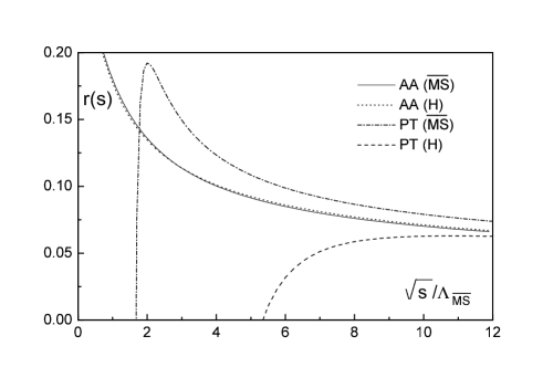
Figure 1: Plot of the QCD correction $r_{f=3}(s)$ calculated in the cases of perturbation theory (PT) and the analytic approach (AA) in two different RS’s with approximately the same cancellation index $C_{R}\simeq 2$: H and $\overline{\rm MS}$.

In Fig. 1, we plot the QCD correction $r_{f=3}(s)$ as a function of $\sqrt{s}/\Lambda_{\overline{\rm MS}}~{}$ for these two schemes in the usual treatment, as it was considered, e.g., in Refs. racz ; ckl ; ms and within the AA. One can see that the analytically improved result for $R(s)$ obeys a stable behavior for the whole interval of energies being practically scheme-independent.

4. To incorporate threshold effects and compare our results with experiment, we use for the cross-section ratio an approximate expression – see Ref. PQW

$$\tilde{R}(s)=3\sum_{f}\,Q_{f}^{2}\,\Theta(s-4m_{f}^{2})\,T(v_{f})\,\left[1\,+\,g(v_{f})r_{f}(s)\right]\,,$$ (4)

$$v_{f}=\sqrt{1-4m_{f}^{2}/s},\;T(v)=v(3-v^{2})/2,\;g(v)=\frac{4\pi}{3}\left[\frac{\pi}{2v}-\frac{3+v}{4}\left(\frac{\pi}{2}-\frac{3}{4\pi}\right)\right],$$

and consider the “smeared” quantity

$$R_{\Delta}(q^{2})=\frac{\Delta}{\pi}\int_{0}^{\infty}\,ds\frac{\tilde{R}(s)}{(s-q^{2})^{2}+\Delta^{2}}\,.$$ (5)

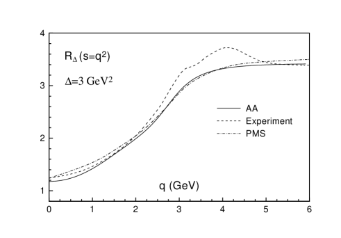
Figure 2: The smeared $e^{+}e^{-}$ annihilation ratio $R_{\Delta}(q^{2})$ vs. $q$.

In Fig. 2 we show smeared experimental data for $R_{\Delta}(q^{2})$ at $\Delta=3\,{\rm GeV}^{2}$ and the third-order PMS curve taken from Ref. ms . In the same figure we plot our three-loop result obtained with the value of the scale parameter as in Ref. pl97 .

5. Now we consider the Adler $D$-function, for which new “experimental” data have been recently obtained in Ref. EJKV98 and we will compare our results with them. It should be noted that a comparison with the $D$-function data determined in the Euclidean region does not require any “smearing procedure” and can be done directly.

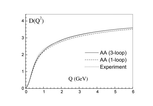
Figure 3: The $D$-function vs. $Q$.

By using Eq. (4), we can derive the Adler function, $D(Q^{2})$. Its low $Q$-shape is sensitive to the light quark mass values. To obtain the best fit, these values have to be chosen near the constituent quark mass values (compare with Ref. jeg96 ). Here, to derive $R_{\Delta}(s)$ and $D(Q^{2})$, we used $m_{u}=m_{d}=250$ MeV, $m_{s}=400$ MeV, $m_{c}=1.35$ GeV, $m_{b}=4.75$ GeV, and $m_{t}=174$ GeV. In Fig. 3 we plot our fresh results for $D$-function calculated via $r_{f}(s)$ in Eq. (4) in the ${\overline{{\rm MS}}}$ scheme. The three-loop curve agrees quite well with the one of Ref. EJKV98 . Note that our description of the $D$-function is RS stable in accordance with general features of the AA.

6. The analytically improved running coupling being a smooth function in the IR region turns out to be remarkably stable with respect to higher loop corrections. Its shape agrees well with the IR integral characteristic extracted from jet physics data. We have found further evidence that our AA reduces the RS dependence drastically: $r_{\rm an}(s)$ thus obtained turns out to be practically scheme-independent in a wide class of RS for the whole energy interval. We have also demonstrated that the AA description agrees with experimental data for the smeared $e^{+}e^{-}$ annihilation ratio and the vector current $D$-function quite well.

The authors would like to thank A.L. Kataev who brought the paper EJKV98 to our attention. We also grateful to him and F. Jegerlehner for useful discussions of the results obtained. The partial support of the RFFI grants Nos. 96-15-96030, 99-01-00091, and INTAS 96-0842 is appreciated.

References

- (1) N.N. Bogoliubov, A.A. Logunov and D.V. Shirkov, Sov. Phys. JETP 10 (1959) 574.
- (2) D.V. Shirkov and I.L. Solovtsov, JINR Rapid Comm. No. 2[76]-96, 5, hep-ph/9604363.
- (3) D.V. Shirkov and I.L. Solovtsov, Phys. Rev. Lett. 79 (1997) 1209; hep-ph/9704333.
- (4) D.V. Shirkov, Nucl. Phys. (Proc. Suppl.) B 64 (1998) 106, hep-ph/9708480.
- (5) D.V. Shirkov, Teor. Mat. Fizika 119 (1999) 55, hep-th/9810246.
- (6) K.A. Milton, I.L. Solovtsov and O.P. Solovtsova, Phys. Lett. B 415 (1997) 104, hep-ph/9706409.
- (7) K.A. Milton, I.L. Solovtsov, and O.P. Solovtsova, Phys.Lett. B 439 (1998) 421, hep-ph/9809510.
- (8) I.L. Solovtsov and D.V. Shirkov, Phys. Lett. B 442 (1998) 344, see also hep-ph/9711251.
- (9) P.A. Raczka and A. Szymacha, Phys. Rev. D 54 (1996) 3073.
- (10) K.A. Milton and I.L. Solovtsov, Phys. Rev. D 55 (1997) 5295.
- (11) P.A. Raczka, Z. Phys. C 65 (1995) 481.
- (12) P.M. Stevenson, Phys. Rev. D 23 (1981) 2916.
- (13) J. Chyla, A.L. Kataev and S.A. Larin, Phys. Lett. B 267 (1991) 269.
- (14) A.C. Mattingly and P.M. Stevenson, Phys. Rev. Lett. 69 (1992) 1320; Phys. Rev. D 49 (1994) 437.
- (15) E.C. Poggio, H.R. Quinn and S. Weinberg, Phys. Rev. D 13 (1976) 1958.
- (16) S. Eidelman, F. Jegerlehner, A.L. Kataev, and O. Veretin, Preprint DESY 98-206, hep-ph/9812521.
- (17) F. Jegerlehner, Nucl. Phys. (Proc. Suppl.) C 51 (1996) 131; DESY Preprint 96-121, June 1996; hep-ph/9606484.