CERN-TH/99-172

Saclay-T99/059

hep-ph/9906485

Ultrasoft Amplitudes in Hot QCD
Jean-Paul BLAIZOT

Service de Physique Théorique, CE-Saclay
91191 Gif-sur-Yvette, France and

Edmond IANCU

Theory Division, CERN
CH-1211, Geneva 23, Switzerland

By using the Boltzmann equation describing the relaxation of colour excitations in the QCD plasma, we obtain effective amplitudes for the ultrasoft colour fields carrying momenta of order $g^{2}T$. These amplitudes are of the same order in $g$ as the hard thermal loops (HTL), which they generalize by including the effects of the collisions among the hard particles. The ultrasoft amplitudes share many of the remarkable properties of the HTL’s: they are gauge invariant, obey simple Ward identities, and, in the static limit, reduce to the usual Debye mass for the electric fields. However, unlike the HTL’s, which correspond effectively to one-loop diagrams, the ultrasoft amplitudes resum an infinite number of diagrams of the bare perturbation theory. By solving the linearized Boltzmann equation, we obtain a formula for the colour conductivity which accounts for the contributions of the hard and soft modes beyond the leading logarithmic approximation.

PACS numbers: 11.10.Wx, 12.38.Mh, 12.38.Cy, 52.60.+h

To appear in Nuclear Physics B

1 Introduction

In recent years, kinetic theory has proven to be a powerful tool to construct effective theories for the soft fields in ultrarelativistic plasmas. Thus, the effective theory at the scale $gT$ follows from a collisionless kinetic equation, of the Vlasov type [1]. The effective theory at the scale $g^{2}T$ is generated by a Boltzmann equation which includes a collision term for colour relaxation [2, 3, 4, 5]. (Here, $T$ is the temperature, and $g$ is the coupling constant, assumed to be small.) The kinetic description relies on the separation of scales between single-particle and collective excitations. This allows for kinematical approximations which, like the relevant scales themselves, are controlled by powers of $g$. By using these approximations, kinetic equations have been rigorously constructed from the quantum equations of motion [1, 2, 4, 6], thus providing justification for numerous previous works using ad hoc transport equations inspired by classical physics [7, 8, 9, 10, 11, 12, 5, 13, 14]. Previous attempts to derive these equations [15] generally failed to recognize the proper separation of scales which turns out to be essential in order to control the gauge invariance of the approximations involved.

The single-particle excitations of the QCD plasma are hard transverse gluons with typical momenta $k\sim T$. The soft fields are colour fields $A^{\mu}_{a}(x)$ with momenta of the order $gT$ or less. When acting on the hard particles, these soft fields induce longwavelength ($\lambda\mathrel{\hbox to0.0pt{\raise 2.20013pt\hbox{$>$}\hss}{\lower 2.20013pt\hbox{$\sim$}}}1/gT$) collective excitations, with $\lambda$ much larger than the mean interparticle distance $\bar{r}\sim 1/T$ [16, 17, 6]. In the framework of the kinetic theory, these excitations are described by a colour density matrix $\delta N_{ab}({\bf k},x)$ to which the soft fields $A^{\mu}_{a}(x)$ couple via kinetic equations. By solving these equations, one can express $\delta N_{ab}$ as a functional of the fields $A^{\mu}_{a}$. The corresponding colour current (with $v^{\mu}=(1,{\bf k}/k)$) :

$$j_{a}^{\mu}(x)\equiv 2g\int{{\rm d}^{3}k\over(2\pi)^{3}}\,v^{\mu}\,{\rm Tr}\,\Bigl{(}T^{a}\delta N({\bf k},x)\Bigr{)},$$ (1.1)

acts as a generating functional for the (equilibrium) amplitudes of the soft fields [1, 6]:

$$j^{a}_{\mu}\,=\,\Pi_{\mu\nu}^{ab}A_{b}^{\nu}+{1\over 2}\,\Gamma_{\mu\nu\rho}^{abc}A_{b}^{\nu}A_{c}^{\rho}+\,...$$ (1.2)

Here, $\Pi_{\mu\nu}^{ab}=\delta^{ab}\Pi_{\mu\nu}$ is the soft polarization tensor, and the other terms represent vertex corrections. These are the amplitudes which define the effective theory for the soft fields. When applied to colour excitations at the scale $gT$ [1, 6, 16], this strategy provides the so-called “hard thermal loops” (HTL) [18, 19, 17]. It is our purpose in this paper to generalize this strategy to the ultrasoft scale $g^{2}T$, and construct the corresponding amplitudes.

Remarkably, to the order of interest the density matrix can be parametrized as:

$$\delta N_{ab}({\bf k},x)\,=\,-gW_{ab}(x,{\bf v})\,({\rm d}N_{0}/{\rm d}k),$$ (1.3)

where $N_{0}(k)\equiv 1/({\rm e}^{\beta k}-1)$ is the Bose-Einstein thermal distribution, and $W(x,{\bf v})\equiv W_{a}(x,{\bf v})T^{a}$ is a colour matrix in the adjoint representation which depends upon the velocity ${\bf v}={\bf k}/k$ (a unit vector), but not upon the magnitude $k=|{\bf k}|$ of the momentum. Then, the kinetic equations are written as equations for $W_{a}(x,{\bf v})$.

Let us briefly recall the situation at the scale $gT$. The relevant kinetic equation is a non-Abelian generalization of the Vlasov equation [1]:

$$(v\cdot D_{x})^{ab}W_{b}(x,{\bf v}) = {\bf v}\cdot{\bf E}^{a}(x).$$ (1.4)

It differs from the corresponding Abelian equation, namely (with $W(x,{\bf v})$ a fluctuation in the electric charge density)

$$(v\cdot\partial_{x})W(x,{\bf v}) = {\bf v}\cdot{\bf E}(x),$$ (1.5)

merely by the repacement of the ordinary (soft) derivative $\partial_{x}\sim gT$ by the covariant one $D_{x}=\partial_{x}+igA$. Accordingly, the soft gluon polarization tensor derived from eq. (1.4) is formally identical to the photon polarization tensor obtained from eq. (1.5). In addition, eq. (1.4) also generates, through the covariant derivative, an infinite series of gluon vertices. These are the HTL’s alluded to before, corresponding to one-loop diagrams with soft external lines and hard internal momenta [18, 19]. Note that the kinetic equation (1.5) isolates directly the dominant contributions of such diagrams, in a gauge invariant manner.

This close similitude between the response of Abelian and non-Abelian plasmas to longwavelength perturbations disappears, however, when going to very soft perturbations, where collisions start to play a role. The effects of the collisions depend upon the specific excitations one is looking at. To give a crude estimate of these effects, one may use the relaxation time approximation, where the kinetic equation is written as

$$(v\cdot D_{x})^{ab}W_{b}(x,{\bf v}) = {\bf v}\cdot{\bf E}^{a}(x)\,-\,{W^{a}(x,{\bf v})\over\tau_{col}},$$ (1.6)

and $\tau_{col}$ is the typical relaxation time for small off-equilibrium colour fluctuations. Like the damping rate $\gamma$ for hard quasiparticles [20, 21, 22, 23], to which it is intimately related (see below), the relaxation of colour is dominated by the singular forward scattering (i.e., by soft momentum transfers in the collision in Fig. 1), which yields $\tau_{col}\sim 1/\gamma\sim 1/(g^{2}T\ln(1/g))$ [8, 9]. Then, eq. (1.6) shows that the effect of the collisions become a leading order effect for inhomogeneities at the scale $\partial_{x}\sim g^{2}T$, or less. This should be contrasted with the case of colourless fluctuations, for instance fluctuations in the momentum or the electric charge distributions, where the typical relaxation time is much larger, $\tau_{el}\sim 1/(g^{4}T\ln(1/g))$, as it requires large angle scattering [7, 11, 12].

For colour fluctuations at the scale $g^{2}T$, it is further convenient to constrain the amplitudes of the associated mean fields such as $|A^{\mu}_{a}|\sim gT$; then the two terms of the ultrasoft covariant derivative are of the same order in $g$ (namely $\partial_{x}\sim gA\sim g^{2}T$) and, in the derivation of the kinetic equations, one can consistently preserve gauge symmetry with respect to the background field [4]. There is another reason which makes this constraint interesting: $|A^{\mu}_{a}|\sim gT$ is the typical amplitude of the thermal fluctuations at the scale $g^{2}T$ [24]. These fluctuations have relatively large amplitudes because of Bose-Einstein enhancement, and their dynamics is fully non-linear; as a result, perturbation theory breaks down at the scale $g^{2}T$ [17, 25]. Moreover, these large amplitude fluctuations make it impossible to give a gauge independent meaning to inhomogeneities on scales much larger than $1/g^{2}T$. A convenient strategy to deal with this situation is to observe that the soft modes can be treated as classical fields, precisely because of their large occupation numbers [26, 25, 27, 2] (and references therein). Then, the non-perturbative dynamics can be studied via classical lattice simulations of the effective theory for soft fields [28, 29, 30].

In order to explicitly construct this theory, however, one needs to go beyond the relaxation time approximation (1.6). In fact, eq. (1.6) is inconsistent with gauge symmetry, as it leads to a colour current which is not conserved. The correct kinetic equation, as derived in [2, 4] (see also Refs. [3, 5, 13]), involves a more complicated collision term, which is local in $x$, but non-local in ${\bf v}$ (see eq. (2) below). Since this collision term is saturated by soft momentum transfers (it is logarithmically sensitive to all momenta $q\mathrel{\hbox to0.0pt{\raise 2.20013pt\hbox{$<$}\hss}{\lower 2.20013pt\hbox{$\sim$}}}gT$), it is useful to isolate the ultrasoft ($q\sim g^{2}T$) background fields from the soft ($g^{2}T\mathrel{\hbox to0.0pt{\raise 2.20013pt\hbox{$<$}\hss}{\lower 2.20013pt\hbox{$\sim$}}}q\mathrel{\hbox to0.0pt{\raise 2.20013pt\hbox{$<$}\hss}{\lower 2.20013pt\hbox{$\sim$}}}gT$) gluons exchanged in the collisions by introducing an intermediate scale $\mu$ such as $g^{2}T\ll\mu\ll gT$ (e.g., $\mu\simeq g^{2}T\ln(1/g)$). Then, the Boltzmann equation generates an effective theory for the ultrasoft ($q<\mu$) fields, corresponding to “integrating out” the hard and soft ($q>\mu$) fields to leading order in perturbation theory [2, 4] (see also Secs. 2 and 3.2 below for a discussion of the relevant approximations). The scale $\mu$ acts as an infrared (IR) cutoff for the collision integral, and as an ultraviolet (UV) cutoff for the effective theory, and it must cancel in any complete calculation of ultrasoft correlation functions (a cancellation referred to as matching).

It is our purpose in this paper to study the contribution of hard and soft fields to the amplitudes with ultrasoft external fields (ultrasoft amplitudes in brief) by an analysis of the solution to the Boltzmann equation.

In previous applications of the latter — namely, to the calculation of the (transverse) colour conductivity to leading logarithmic accuracy [8, 9, 2, 3] —, the non-local piece of the collision term turned out not to be important. But this was specific to that particular approximation, which has ignored all the non-local and non-linear effects in the problem (essentially because the drift term $v\cdot D_{x}\sim g^{2}T$ has been neglected as compared to $\gamma\sim g^{2}T\ln(1/g)$; see Sec. 3.4 for more details). In that situation, the ultrasoft amplitudes in eq. (1.2) collapsed to a single, local quantity, namely the colour conductivity.

Our intention here is to go beyond this leading logarithmic approximation and study the generic ultrasoft amplitudes generated by the Boltzmann equation for colour relaxation. This includes, in particular, the non-local effects in space and time, as governed by the drift term $v\cdot D_{x}$, and also the non-local effects in ${\bf v}$ coming from the collision term. Because of the latter, the Boltzmann equation cannot be exactly solved in general. Thus, we will not be able to provide full expressions for the ultrasoft amplitudes except in some simple limits (cf. Sec. 4.2). Still, many of the important properties of these amplitudes can be inferred from an analysis of the Boltzmann equation (cf. Secs. 3.1, 3.3 and 4 below). Moreover, some formal solutions can also be obtained, by iterations, and this is specially useful for comparison with diagrammatic perturbation theory (cf. Secs. 3.2 and 3.3). The Boltzmann equation accomplishes a non-trivial resummation of the perturbative expansion, made evident by the derivation of this equation from quantum field theory [4], where the collision term has a direct diagrammatic interpretation (see Sec. 2 below for a short review of this derivation).

Let us briefly enumerate here the main properties of the ultrasoft amplitudes, to be derived below in this paper: For generic external momenta of order $g^{2}T$, these amplitudes are of the same order in $g$ as the HTL’s, which they generalize by taking into account the effects of the collisions. The ultrasoft amplitudes share many of the remarkable properties of the HTL’s: i) they are non-perturbative, in the sense that in the kinematical regime of interest ($\omega\ll p\mathrel{\hbox to0.0pt{\raise 2.20013pt\hbox{$<$}\hss}{\lower 2.20013pt\hbox{$\sim$}}}g^{2}T$), they are as large as the corresponding tree-level amplitudes; ii) they are gauge-fixing independent, as they involve only collisions among on-shell, hard, transverse gluons, iii) they satisfy simple Ward identities, which express the conservation of the colour current; iv) in the static limit $\omega\to 0$, they reduce to the usual Debye mass term $m_{D}^{2}=g^{2}NT^{2}/3$ for the electric fields. That is, to the order of interest, collisions do not modify Debye screening (see also Ref. [31], and Sec. 3.3 below for more details).

On the other hand, there are also significant differences with respect to the HTL’s: i) The ultrasoft amplitudes have no Abelian counterpart: in QED, the effects of the collisions become important only at the scale $e^{4}T$ (see also Sec. 2 below). ii) Unlike the HTL’s, which correspond to one-loop Feynman graphs, the ultrasoft amplitudes receive contributions from an infinite series of multi-loop diagrams, with a specific structure (essentially, chains of ladder diagrams). Recently, the first few such diagrams for the polarization tensor have been explicitly computed by Bödeker [32], with results which agree with the (first order iteration of the) solution to the Boltzmann equation. But it is clear that, in general, computing directly these diagrams would be a tedious exercice, especially since important cancellations occur among the various graphs [4, 32]; this will be further discussed in Secs. 3.2 and 4.1 below. iii) The resummation of the collision effects drastically modify the longwavelength behaviour of the transverse colour conductivity $\sigma_{T}(\omega=0,p\to 0)$: the would-be divergence of the HTL result for $\sigma_{T}$, namely $\sigma_{T}^{(0)}\propto m_{D}^{2}/p$, is now screened away by $\gamma$, with the net result that $\sigma_{T}(\omega=0,p\to 0)=m_{D}^{2}/3(\gamma-\delta)$. Here $\delta$ is a term of order $g^{2}T$ (and which satisfies $|\delta|<\gamma$), to be computed in Sec. 4.2 below. iv) For ultrasoft momenta $p\sim g^{2}T$, the above formula for $\sigma_{T}$ holds up to corrections of ${\rm O}(\ln^{-2})$ (with $\ln\equiv\ln(1/g)$).

Figure 1: Elastic scattering in the (resummed) Born approximation. The continuous lines refer to hard gluons (these are off-equilibrium propagators), while the wavy line is the soft gluon exchanged in the collision. The blob stands for HTL resummation.

2 The Boltzmann equation

In this section, we review the main features of the Boltzmann equation for colour relaxation which was recently derived in Ref. [4]. There are no new results to be reported here, but the equations derived in [4] will be presented in a slightly different way, to better emphasize the difference between coloured and colourless excitations, and also between Abelian and non-Abelian gauge theories. Moreover, the diagrammatic representation of the collision term will be explained in more detail, in order to facilitate the discussion of the diagrammatic interpretation of the ultrasoft amplitudes, in Sec. 3.2 below.

The space-time inhomogeneities in the distribution of the hard particles (transverse gluons) are described by a density matrix $\delta\acute{G}_{ab}(k,x)$ where the momentum $k$ is hard ($k\sim T$) and on-shell ($k_{0}^{2}={\bf k}^{2}$), and the derivative $\partial_{x}$ is ultrasoft ($\partial_{x}\sim g^{2}T$). Below, we shall be interested either in colourless fluctuations (in which case $\delta\acute{G}_{ab}=\delta_{ab}\delta\acute{G}$), or in coloured ones in the adjoint representation (such as $\delta\acute{G}_{ab}=if^{abc}\delta\acute{G}_{c}$). Also, we shall find convenient to use the following parametrization for the density matrix, where the on-shell structure is explicit:

$$\delta\acute{G}_{ab}(k,x) \equiv -\rho_{0}(k)W_{ab}(k,x)\,{{\rm d}N_{0}\over{\rm d}k_{0}}$$ (2.1)

$$= \beta\rho_{0}(k)W_{ab}(k,x)\,N_{0}(k_{0})[1+N_{0}(k_{0})].$$

In this equation, $N_{0}(k_{0})=1/({\rm e}^{\beta k_{0}}-1)$ and $\rho_{0}(k)=2\pi\epsilon(k_{0})\delta(k^{2})$ are, respectively, the thermal distribution and the spectral density for hard transverse gluons, and the new function $W_{ab}(k,x)$ has support only at the mass-shell: $W_{ab}(k,x)=\theta(k_{0})W_{ab}({\bf k},x)+\theta(-k_{0})W_{ba}(-{\bf k},x)$. [The density matrix $\delta N_{ab}({\bf k},x)$ in the Introduction, eq. (1.3), is related to the function $W_{ab}({\bf k},x)$ by $\delta N_{ab}({\bf k},x)=-W_{ab}({\bf k},x)({\rm d}N_{0}/{\rm d}k)$.]

The Boltzmann equation is the kinetic equation satisfied by the density matrix to leading order in $g$ [4]. It reads (in matrix notations):

$$2\Bigl{[}k\cdot D_{x},\,\delta\acute{G}(k,x)\Bigr{]}\,-\,2gk^{\mu}F_{\mu\nu}(x)\partial^{\nu}_{k}G_{0}^{<}(k)\,=\,C(k,x).$$ (2.2)

In the l.h.s., $k\cdot D_{x}$ is the gauge-covariant drift operator, with $D^{\mu}\equiv\partial^{\mu}+igA^{\mu}$ and $\partial_{x}\sim gA\sim g^{2}T$, so that $D_{x}={\rm O}(g^{2}T)$; $k^{\mu}F_{\mu\nu}(x)\partial^{\nu}_{k}$, with $F_{\mu\nu}\equiv[D_{\mu},D_{\nu}]/ig$, is the “force” term acting on the equilibrium correlation function $G^{<}_{0}(k)$:

$$G^{<}_{0}(k)\,\equiv\,\rho_{0}(k)N_{0}(k_{0}),\qquad G^{>}_{0}(k)\equiv\rho_{0}(k)[1+N_{0}(k_{0})].$$ (2.3)

(The second function $G^{>}_{0}(k)$ will be needed below.)

In the r.h.s. of eq. (2.2), $C(k,x)$ is the collision term associated to the one-gluon exchange process depicted in Fig. 1. A priori, all the lines in this figure (that is, both the external lines associated with the colliding particles, and the wavy line associated to the exchanged gluon) are off-equilibrium propagators. However, to the order of interest, the collision term can be linearized with respect to the off-equilibrium fluctuations in the propagators of the external lines, and the internal propagator can be taken to be the equilibrium propagator. Since the collision term for colour relaxation is dominated by soft momentum transfers ($g^{2}T\mathrel{\hbox to0.0pt{\raise 2.20013pt\hbox{$<$}\hss}{\lower 2.20013pt\hbox{$\sim$}}}q\mathrel{\hbox to0.0pt{\raise 2.20013pt\hbox{$<$}\hss}{\lower 2.20013pt\hbox{$\sim$}}}gT$) [8, 9, 2, 3, 4], the propagator of the exchanged gluon has to be dressed with the corresponding hard thermal loop [16, 17].

Figure 2: Self-energy describing collisions in the (resummed) Born approximation. All the lines represent off-equilibrium propagators. The continuous lines refer to the hard colliding particles in Fig. 1. The wavy lines with a blob denote soft gluon propagators dressed by the screening effects.

The scattering process in Fig. 1 can be associated to the collisional self-energy in Fig. 2 (see Ref. [4] for more details on the formalism). Upon linearization, this leads to the four processes displayed in Fig. 3. Each diagram involves fluctuations in one of the four external lines in Fig. 1. Thus, $C=C_{1}+C_{2}+C_{3}+C_{4}$, where $C_{1}(k,x)$ involves the fluctuations $\delta\acute{G}(k,x)$ in the incoming field with momentum ${\bf k}$ (Fig. 3.a), and $C_{2}$, $C_{3}$ and $C_{4}$ involve fluctuations along the lines with momenta ${\bf k}^{\prime}$, ${\bf p}$ and ${\bf p}^{\prime}$ (Figs. 3.b, c and d, respectively). In these figures, the off-equilibrium propagators are marked with a cross; all the other lines denote equilibrium propagators. In particular, $C_{1}(k,x)=-\Gamma(k)\,\delta\acute{G}(k,x)$, where

$$\Gamma(k)\equiv\Sigma^{<}_{eq}(k)-\Sigma^{>}_{eq}(k)=-2\,{\rm Im}\Sigma_{R}(k)\,,$$ (2.4)

is the quantity which determines the quasiparticle damping rate $\gamma\equiv\Gamma(k_{0}=k)/(4k)\,\sim\,g^{2}T\ln(1/g)$ [18, 20, 21, 22].

By using the parametrization (2.1) for the density matrix, the (linearized) collision term can be compactly written as:

Figure 3: Pictorial representation of the linearized collision term. Each one of the four diagrams correspond to off-equilibrium fluctuations in one of the colliding fields (the one which is marked with a cross). All the unmarked propagators are in equilibrium.

$$C_{ab}(k,x) = -\int{\rm d}{\cal T}\left|{\cal M}_{pk\to p^{\prime}k^{\prime}}\right|^{2}\,N_{0}(k_{0})\,N_{0}(p_{0})\,[1+N_{0}(k^{\prime}_{0})]\,[1+N_{0}(p^{\prime}_{0})]$$ (2.5)

$$\qquad\times\Bigl{\{}N\Bigl{(}NW_{ab}(k,x)-(T^{a}T^{b})_{cd}W_{cd}(k^{\prime},x)\Bigr{)}\,+$$

$$\qquad\,\,\,\,\,\,\,\,+\,(T^{a}T^{b})_{c\bar{c}}(T^{c}T^{\bar{c}})_{d\bar{d}}\Bigl{(}W_{\bar{d}d}(p,x)-W_{d\bar{d}}(p^{\prime},x)\Bigr{)}\Bigr{\}}.$$

In this equation, $\left|{\cal M}_{pk\to p^{\prime}k^{\prime}}\right|^{2}$ is the matrix element squared corresponding to the one-gluon exchange depicted in Fig. 1, and ${\rm d}{\cal T}$ is a compact notation for the measure of the phase-space integral:

$$\int{\rm d}{\cal T}\,\equiv\,\beta\int{{\rm d}^{4}p\over(2\pi)^{4}}\int{{\rm d}^{4}q\over(2\pi)^{4}}\,\rho_{0}(k)\rho_{0}(p)\rho_{0}(p+q)\rho_{0}(k-q).$$ (2.6)

The four terms within the braces in eq. (2.5) are in one to one correspondance with the diagrams 3.a, b, c and d. The appearance of the matrix element squared, and also of the various equilibrium statistical factors in eq. (2.5), is familiar. What is specific to the problem at hand is the colour structure in eq. (2.5), which is at the origin of an important difference between coloured and colourless excitations:

Consider first the case of a colourless fluctuation, for which $\delta\acute{G}_{ab}=\delta_{ab}\delta\acute{G}$, and $W_{ab}=\delta_{ab}W$. The various colour traces in eq. (2.5) are trivial (e.g., $(T^{a}T^{b})_{cc}=N\delta_{ab}$), so that $C_{ab}=\delta_{ab}C$, with

$$C(k,x) = -N^{2}\int{\rm d}{\cal T}\left|{\cal M}_{pk\to p^{\prime}k^{\prime}}\right|^{2}\,N_{0}(k_{0})\,N_{0}(p_{0})\,[1+N_{0}(k^{\prime}_{0})]\,[1+N_{0}(p^{\prime}_{0})]$$ (2.7)

$$\qquad\times\Bigl{\{}W(k,x)-W(k^{\prime},x)+W(p,x)-W(p^{\prime},x)\Bigr{\}}.$$

This is the standard collision term for one-gluon exchange used in previous applications of kinetic theory to the hot quark-gluon plasma or to the electroweak plasma [12].

What is remarkable about eq. (2.7) is that the corresponding phase-space integral is dominated by relatively hard momentum transfers $gT\mathrel{\hbox to0.0pt{\raise 2.20013pt\hbox{$<$}\hss}{\lower 2.20013pt\hbox{$\sim$}}}q\mathrel{\hbox to0.0pt{\raise 2.20013pt\hbox{$<$}\hss}{\lower 2.20013pt\hbox{$\sim$}}}T$, even though each of the four individual terms in the r.h.s. is actually saturated by soft momenta. This is a consequence of the cancellation of the leading infrared contributions among the various terms [4]. For instance, for soft $q$, $W(k^{\prime},x)\equiv W(k-q,x)\approx W(k,x)$, so that the IR contributions to the first two terms in eq. (2.7) cancel each other. This corresponds to a cancellation among the graphs displayed in Figs. 3.a and b, to be further discussed in Sec. 3.2 below. A similar cancellation occurs between the last two terms in eq. (2.7), namely $W(p,x)$ and $W(p^{\prime},x)$. Thus, in order to see the leading IR ($q\ll T$) behaviour of the full integrand in eq. (2.5), one has to expand $W(k^{\prime},x)$ and $W(p^{\prime},x)$ to higher orders in $q$. This generates extra factors of $q$ which remove the most severe IR divergences in the collision integral. (This is the familiar $(1-\cos\theta)$ factor of the “transport cross section” [33].) As a result, the typical rate involved in the calculation of the transport coefficients like the shear viscosity is $\sim\,g^{4}T\ln(1/g)$, where the logarithm originates from screening effects at the scale $gT$ [7, 11]. This is suppressed by one power of $\alpha\equiv g^{2}/4\pi$ with respect to the damping rate $\gamma\,\sim\,g^{2}T\ln(1/g)$.

Consider now the case of colour fluctuations corresponding to a density matrix $W(k,x)$ of the form $W(k,x)\equiv W_{a}(k,x)T^{a}$. The colour algebra in eq. (2.5) can be performed with the following identities:

$${\rm Tr}(T^{a}T^{b}T^{c})\,=\,if^{abc}\,{N\over 2}\,,\qquad(T^{a}T^{b})_{c\bar{c}}(T^{c}T^{\bar{c}})_{d\bar{d}}(T^{e})_{\bar{d}d}\,=\,if^{abe}\,{N^{2}\over 4}\,.$$ (2.8)

The resulting collision term is of the form $C=C_{a}T^{a}$ with

$$C_{a}(k,x) = -N^{2}\int{\rm d}{\cal T}\left|{\cal M}_{pk\to p^{\prime}k^{\prime}}\right|^{2}\,N_{0}(k_{0})\,N_{0}(p_{0})\,[1+N_{0}(k^{\prime}_{0})]\,[1+N_{0}(p^{\prime}_{0})]$$ (2.9)

$$\qquad\times\left\{W_{a}(k,x)-\,{1\over 2}\,W_{a}(k^{\prime},x)-\,{1\over 4}\Bigl{(}W_{a}(p,x)+W_{a}(p^{\prime},x)\Bigr{)}\right\}.$$

There are two notable differences with respect to eq. (2.7):
i) The first two terms within the braces enter with a relative factor 1/2, so they do not cancel each other when $q\to 0$ :

$$W_{a}(k,x)-\,{1\over 2}\,W_{a}(k-q,x)\,\simeq\,\,{1\over 2}\,W_{a}(k,x).$$ (2.10)

Rather, their overall contribution is half the corresponding contribution of the first term alone, that is, $\Gamma(k)/2$.
ii) The last two terms in eq. (2.9) enter with a factor $1/4$ and add each other. This is so because the colour matrix $W_{\bar{d}d}(p,x)$ in eq. (2.5) is antisymmetric, rather than symmetric, as it is for colourless fluctuations. Accordingly, for soft $q$,

$${1\over 4}\Bigl{(}W_{a}(p,x)+W_{a}(p+q,x)\Bigr{)}\,\simeq\,\,{1\over 2}\,W_{a}(p,x).$$ (2.11)

Thus, for colour fluctuations, the colour structure of the collision term prevents a complete cancellation of the leading infrared contributions: like the damping rate, the collision term for colour relaxation is saturated by soft momentum transfers ($g^{2}T\mathrel{\hbox to0.0pt{\raise 2.20013pt\hbox{$<$}\hss}{\lower 2.20013pt\hbox{$\sim$}}}q\mathrel{\hbox to0.0pt{\raise 2.20013pt\hbox{$<$}\hss}{\lower 2.20013pt\hbox{$\sim$}}}gT)$, for which eqs. (2.10) and (2.11) hold and the collision term (2.9) simplifies to [3, 4]:

$$C_{a}(k,x)\simeq-\,{N^{2}\over 2}\int{\rm d}{\cal T}\left|{\cal M}_{pk\to p^{\prime}k^{\prime}}\right|^{2}\,{{\rm d}N_{0}\over{\rm d}k_{0}}\,{{\rm d}N_{0}\over{\rm d}p_{0}}\,\left\{W_{a}(k,x)\,-\,W_{a}(p,x)\right\}.$$ (2.12)

In the same approximation, the matrix element $|{\cal M}|^{2}$ can be evaluated as:

$$|{\cal M}|^{2}\,=\,16g^{4}\varepsilon_{k}^{2}\varepsilon_{p}^{2}\,\Big{|}{}^{*}{\cal D}_{l}(q)+({\bf\hat{q}\times v})\cdot({\bf\hat{q}\times v}^{\prime})\,{}^{*}{\cal D}_{t}(q)\Big{|}^{2},$$ (2.13)

where ${\bf v}\equiv\hat{\bf k}$, ${\bf v}^{\prime}\equiv\hat{\bf p}$, and ${}^{*}{\cal D}_{l}$ and ${}^{*}{\cal D}_{t}$ are the longitudinal (or electric) and the transverse (or magnetic) components of the (retarded) gluon propagator, in the hard thermal loop approximation [16, 17]. The phase-space measure (2.6) can be similarly simplified. This eventually yields a simpler equation for the density matrix $W_{a}({\bf k},x)$ which, remarkably, is consistent with $W_{a}({\bf k},x)$ being independent of the magnitude $k\equiv|{\bf k}|$ of the hard momentum. That is,

$$W_{a}({\bf k},x) \equiv gW_{a}(x,{\bf v}),$$ (2.14)

where ${\bf v}\equiv{\bf k}/k$ is the velocity of the termal particle (a unit vector), and a factor of $g$ has been introduced to keep in line with the notations of Ref. [4].

Finally. the Boltzmann equation, written as an equation for $W_{a}(x,{\bf v})$, reads [4]:

$$(v\cdot D_{x})^{ab}W_{b}(x,{\bf v}) = {\bf v}\cdot{\bf E}^{a}(x)-m_{D}^{2}{g^{2}NT\over 2}\int{{\rm d}\Omega^{\prime}\over 4\pi}\,\Phi({\bf v\cdot v}^{\prime})\Bigl{\{}W^{a}(x,{\bf v})-W^{a}(x,{\bf v}^{\prime})\Bigr{\}}.$$

The angular integral above runs over all the directions of the unit vector ${\bf v}^{\prime}$, and $m_{D}^{2}$ is the Debye mass squared:

$$m^{2}_{D}\,\equiv\,-\,{g^{2}N\over\pi^{2}}\int_{0}^{\infty}{\rm d}p\,p^{2}\,{{\rm d}N_{0}\over{\rm d}p}\,=\,{g^{2}NT^{2}\over 3}\,.$$ (2.16)

Furthermore:

$$\Phi({\bf v\cdot v}^{\prime})\equiv(2\pi)^{2}\int{{\rm d}^{4}q\over(2\pi)^{4}}\,\delta(q_{0}-{\bf q\cdot v})\delta(q_{0}-{\bf q\cdot v}^{\prime})\Big{|}{}^{*}{\cal D}_{l}(q)+({\bf v}_{t}\cdot{\bf v}_{t}^{\prime})\,{}^{*}{\cal D}_{t}(q)\Big{|}^{2},\,\,\,$$ (2.17)

with the two delta functions expressing the energy conservation at the two vertices of the scattering process in Fig. 1. Up to a normalization, the function $\Phi({\bf v\cdot v}^{\prime})$ represents the cross section for the collision between two hard particles with velocities ${\bf v}$ and ${\bf v}^{\prime}$ exchanging (in the $t$-channel) a soft (dressed) gluon.

The collision term in eq. (2) involves two pieces: one which is local in ${\bf v}$ (proportional to $W^{a}(x,{\bf v})$), and one which is non-local (involving the kernel $\Phi({\bf v\cdot v}^{\prime})$. The coefficient of the local piece is proportional to $\Gamma$ :

$$m_{D}^{2}\,{g^{2}NT\over 2}\int{{\rm d}\Omega^{\prime}\over 4\pi}\,\Phi({\bf v\cdot v}^{\prime})\,=\,{\Gamma(k_{0}=k)\over 4k}\,\equiv\,\gamma.$$ (2.18)

By using the expression above, we can rewrite the Boltzmann equation (2) in the following way:

$$(v\cdot D_{x})^{ab}W_{b}(x,{\bf v}) = {\bf v}\cdot{\bf E}^{a}(x)-\gamma\Bigl{\{}W^{a}(x,{\bf v})\,-\,\langle W^{a}(x,{\bf v})\rangle\Bigr{\}},$$ (2.19)

which emphasizes the fact that the quasiparticle damping rate $\gamma$ sets the time scale for colour relaxation: $\tau_{col}\sim 1/\gamma\sim 1/(g^{2}T\ln(1/g))$ [8] (see also Sec. 4.2 below). In eq. (2.19) we have introduced a notation which will be used hereafter: for an arbitrary function of ${\bf v}$, say $F({\bf v})$, we denote by $\langle F({\bf v})\rangle$ its angular average with weight function $\Phi({\bf v\cdot v}^{\prime})$:

$$\langle F({\bf v})\rangle\,\equiv\,{\int{{\rm d}\Omega^{\prime}\over 4\pi}\,\Phi({\bf v\cdot v}^{\prime})F({\bf v}^{\prime})\over\int{{\rm d}\Omega^{\prime}\over 4\pi}\,\Phi({\bf v\cdot v}^{\prime})}\,,$$ (2.20)

which is still a function of ${\bf v}$.

We conclude this section by recalling that eq. (2) is invariant under the gauge transformations of the background field, and also with respect to the choice of a gauge for the shortwavelength fluctuations (here, the hard ($k\sim T$) fields which take part in the collective motion and the soft ($g^{2}T\mathrel{\hbox to0.0pt{\raise 2.20013pt\hbox{$<$}\hss}{\lower 2.20013pt\hbox{$\sim$}}}q\mathrel{\hbox to0.0pt{\raise 2.20013pt\hbox{$<$}\hss}{\lower 2.20013pt\hbox{$\sim$}}}gT$) gluons which are exchanged in the collision process). In Ref. [4], eq. (2) was derived in Coulomb gauge, but we expect it to be gauge-fixing independent. Except for the collision term, this has been explicitly verified in [1] (see also Refs. [18, 19]). The collision term should be gauge-fixing independent as well, since it involves only the off-equilibrium fluctuations of the (hard) transverse gluons, together with the (gauge-independent) matrix element squared (2.13). However, an explicit proof comparable to the corresponding one for the non-Abelian Vlasov equation [1] is somewhat tedious: in an arbitrary gauge (e.g., a covariant one), one has to consider collisions involving fictitious degrees of freedom (hard longitudinal gluons and ghosts), and verify that their respective contributions to the collision term mutually cancell.

3 Ultrasoft amplitudes

In this section, we introduce and study the ultrasoft amplitudes, i.e., the contributions to the one-particle irreducible amplitudes with ultrasoft external lines which are obtained from the solution to the Boltzmann equation.

3.1 The induced current

The longwavelength colour fluctuations of the hard particles generate a colour current given by (the factor of 2 below stands for the two transverse polarizations):

$$j^{a}_{\mu}(x)=2g\int{{\rm d}^{4}k\over(2\pi)^{4}}\,k_{\mu}\,{\rm Tr}\,\Bigl{(}T^{a}\delta\acute{G}(k,x)\Bigr{)},$$ (3.1)

which acts as a source in the Yang-Mills equations for the ultrasoft colour fields $A^{\mu}_{a}$:

$$(D^{\nu}F_{\nu\mu})^{a}(x) = j_{\mu}^{a}(x).$$ (3.2)

By using the parametrization (2.1) for the density matrix, one can perform the integral over the radial momentum $k\equiv|{\bf k}|$ to obtain:

$$j^{\mu}_{a}(x) = m_{D}^{2}\int{{\rm d}\Omega\over 4\pi}\,v^{\mu}\,W_{a}(x,{\bf v}),$$ (3.3)

with the Debye mass $m_{D}$ defined in eq. (2.16). By using the equation of motion (2) for $W^{a}(x,{\bf v})$, one can verify that the current (3.3) is covariantly conserved,

$$D_{\mu}j^{\mu}\,=\,0,$$ (3.4)

as necessary for the consistency of the mean field equations of motion (3.2) (recall that $D^{\mu}D^{\nu}F_{\nu\mu}=0$). Indeed, eq. (2) implies:

$$D_{\mu}j^{\mu} = m_{D}^{2}\int{{\rm d}\Omega\over 4\pi}\,{\bf v}\cdot{\bf E}^{a}(x)$$ (3.5)

$$- m_{D}^{4}{g^{2}NT\over 2}\int{{\rm d}\Omega\over 4\pi}\int{{\rm d}\Omega^{\prime}\over 4\pi}\,\Phi({\bf v\cdot v}^{\prime})\Bigl{\{}W^{a}(x,{\bf v})-W^{a}(x,{\bf v}^{\prime})\Bigr{\}},$$

which is zero because both terms in the r.h.s. vanish after the angular integration.

By solving the Boltzmann equation, one can obtain the density matrix $W_{a}(x,{\bf v})$, and therefore also the induced current $j^{\mu}_{a}(x)$, as functionals of the gauge fields $A^{\mu}_{a}(x)$. Since eq. (2) is non-linear with respect to the fields $A^{\mu}_{a}$, the resulting functional $j_{a}^{\mu}[A]$ will be non-linear as well, and can be formally expanded as follows:

$$j^{a}_{\mu}\,=\,\Pi_{\mu\nu}^{ab}A_{b}^{\nu}+{1\over 2}\,\Gamma_{\mu\nu\rho}^{abc}A_{b}^{\nu}A_{c}^{\rho}+\,...$$ (3.6)

The coefficients in this expansion are the one-particle-irreducible amplitudes of the fields $A^{\mu}_{a}$, evaluated in thermal equilibrium [16, 6, 1]. For instance, $\Pi_{\mu\nu}^{ab}=\delta^{ab}\Pi_{\mu\nu}$ is the polarization tensor, $\Gamma_{\mu\nu\rho}^{abc}\equiv if^{abc}\Gamma_{\mu\nu\rho}$ is a correction to the 3-gluon vertex, etc. These amplitudes will be referred to as the ultrasoft amplitudes.

Some of the properties of the ultrasoft amplitudes follow immediately from the previous discussion: For generic momenta of order $g^{2}T$, they are of the same order in $g$ as the hard thermal loops [18, 19, 1, 16, 17, 6], which they generalize by including the effects of the collisions. Furthermore, they are gauge-fixing independent (like the Boltzmann equation itself), indicating that only the physical hard degrees of freedom of the plasma (namely, the on-shell transverse gluons) contribute to these amplitudes. Also, they satisfy simple Ward identities which follow from the conservation law (3.4) by successive differentiations with respect to the fields $A^{\mu}_{a}$. For instance:

$$P^{\mu}\,\Pi_{\mu\nu}(P) = 0,$$

$$P^{\mu}\Gamma_{\mu\nu\rho}(P,Q,R) = \Pi_{\nu\rho}(Q)-\Pi_{\nu\rho}(R)\,.$$ (3.7)

All these properties are, of course, very reminiscent of the hard thermal loops, and, as we shall see later, there are other similarities. But let us first discuss the interpretation of the ultrasoft amplitudes in terms of Feynman diagrams.

3.2 Diagrammatic interpretation of the ultrasoft amplitudes

In this subsection, we discuss the interpretation of the solution to the Boltzmann equation in terms of Feynman diagrams. (See also Refs. [34, 35] for a related analysis in the context of scalar field theory, and Ref. [32] for a recent calculation of some of the diagrams relevant to QCD, namely those in Fig. 8 below.) This analysis will show that, unlike the HTL’s — which correspond to one-loop diagrams [18, 19] —, the ultrasoft amplitudes receive contributions from an infinite set of multi-loop Feynman graphs, which, in the kinematical regime of interest, contribute all at the same order in $g$.

Our discussion here will be only qualitative: we shall not compute Feynman graphs explicitly, but rather rely on the diagrammatic representation of the collision term (cf. Figs. 1, 2 and 3) in order to identify, by iterations, the structure of the diagrams contributing to the ultrasoft amplitudes.

To carry out the analysis, it is convenient to use the original form of the Boltzmann equation, where the collision term is directly related to the self-energy. This is eq. (2.2) with the collision term (2.5), which we rewrite here as follows:

$$\Bigl{[}v\cdot D_{x},\,\delta\acute{G}(k,x)\Bigr{]}\,=\,gv^{\mu}F_{\mu\nu}(x)\partial^{\nu}_{k}G_{0}^{<}(k)\,+\,C(k,x),$$

$$C=C_{1}+C_{2}+C_{3}+C_{4},\qquad C_{1}\,=\,-\,{1\over 2k_{0}}\,\Gamma(k)\,\delta\acute{G}(k,x),$$ (3.8)

where $v^{\mu}=k^{\mu}/k_{0}$, and the four pieces of the collision term correspond, respectively, to the linearized fluctuations depicted in Figs. 3.a, b, c and d. (Note that the present normalization of the collision term differs by a factor $1/2k_{0}$ from the previous one in eq. (2.2).) For comparison with perturbation theory, it is useful to regard the collision term as a “small perturbation” and solve the Boltzmann equation (3.2) formally by iterations.

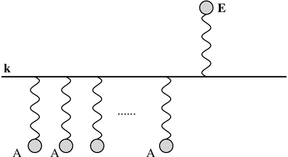
Figure 4: Mean field approximation, or zeroth order iteration for the solution to the Boltzmann equation, eq. (3.9).

The zeroth order iteration is the solution to eq. (3.2) with the collision terms excluded:

$$\delta\acute{G}^{(0)}\,=\,g\,{1\over v\cdot D}\,v^{\mu}F_{\mu\nu}\partial^{\nu}G_{0}^{<}\,.$$ (3.9)

Here, $1/(v\cdot D)$ is a compact, but formal, notation for the retarded Green’s function $\Delta_{R}(x,y;{\bf v})$ of the covariant drift operator $v\cdot D$. This satisfies:

$$(v\cdot D_{x})_{ab}\Delta_{R}^{bc}(x,y;{\bf v})\,=\,\delta^{ac}\delta^{(4)}(x-y),$$ (3.10)

with $\Delta_{R}(x,y;{\bf v})=0$ for $x_{0}<y_{0}$, and has the following expression (with $t\equiv x_{0}-y_{0}$):

$$\Delta_{R}^{ab}(x,y;{\bf v})\,=\,\theta(t)\,\delta^{(3)}\Bigl{(}{{\bf x}}-{{\bf y}}-{\bf v}t\Bigr{)}\,U^{ab}(x,y)\,\equiv\,\Bigl{\langle}x,\,a\Bigl{|}{i\over i(v\cdot D)+i\epsilon}\Bigr{|}y,\,b\Bigr{\rangle},$$ (3.11)

where $U(x,y)$ is the Wilson line connecting the points $x$ and $y\,$:

$$U(x,y)={\rm e}^{-ie\int{\rm d}z^{\mu}A_{\mu}(z)},$$ (3.12)

and the integration path in eq. (3.12) is fixed by the delta function in eq. (3.11). $\Delta_{R}(x,y;{\bf v})$ is the eikonal propagator along the straightline trajectory of velocity ${\bf v}$.

Eq. (3.9) can be given the diagrammatic representation in Fig. 4 where, for more clarity, we have distinguished the insertion of the electric mean field ${\bf E}_{a}$, the “Lorentz force” in the r.h.s. of eq. (3.2), from the insertions of colour fields $A^{\mu}_{a}$ due to the covariant derivative $v\cdot D$ in the l.h.s. Thus, the propagator on the left of the electric field ${\bf E}_{a}$ is the eikonal propagator (3.11), while the propagator on the right is $\partial_{k}G^{<}_{0}(k)$. The corresponding colour current, namely:

$$j^{(0)\,a}_{\mu}(x)=2g\int{{\rm d}^{4}k\over(2\pi)^{4}}\,k_{\mu}\,{\rm Tr}\,\Bigl{(}T^{a}\delta\acute{G}^{(0)}(k,x)\Bigr{)}\,=\,m_{D}^{2}\int{{\rm d}\Omega\over 4\pi}\,\,{v_{\mu}v^{i}E^{i}\over v\cdot D}\,,$$ (3.13)

involves a supplementary integration over the hard momenta $k$, which, in terms of diagrams, corresponds to closing the straight line in Fig. 4 into a hard loop. Thus, the polarisation amplitudes generated by $j^{(0)}_{\mu}$ (cf. eq. (3.6)) are one-loop amplitudes where the internal momentum is hard, while all the external lines are soft (or ultrasoft); some examples are shown in Fig. 5. These are precisely the hard thermal loops, which have been originally computed from one-loop diagrams indeed [18, 19].

Figure 5: Two and four-gluon vertices in the HTL approximation.

As well known, the HTL’s are only a part of the corresponding one-loop amplitudes [18, 19, 17] (namely, the leading order part for soft external lines), and this part is directly singled out by the collisionless kinetic equation, cf. eqs. (3.9) and (3.13) [1, 16, 6].

Consider now the first order iteration of the collision term, which yields:

$$\delta\acute{G}^{(1)}\,=\,{1\over v\cdot D}\,C[\delta\acute{G}^{(0)}]\,.$$ (3.14)

The collision term $C[\delta\acute{G}^{(0)}]$ is illustrated in Fig. 6, which should be compared to Fig. 3.

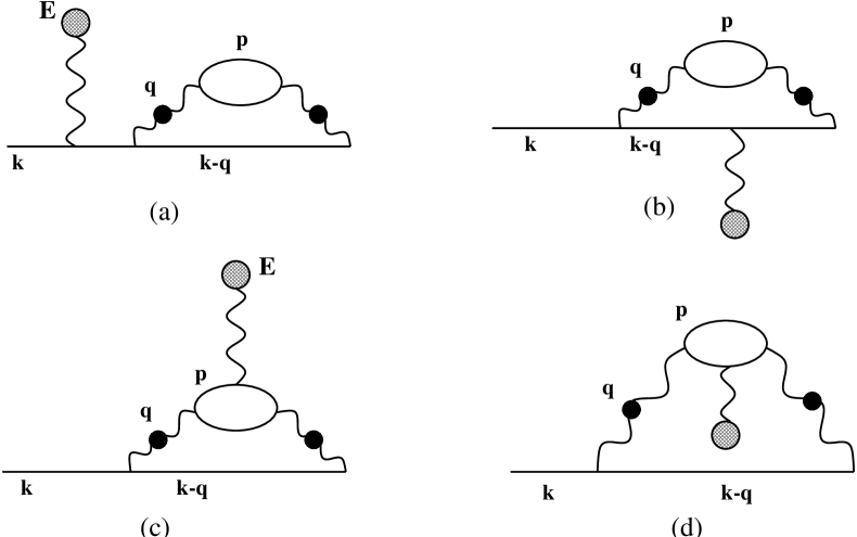
Figure 6: The first order iteration of the collision term $C[\delta\acute{G}^{(0)}]$, to linear order in the background field.

For simplicity, we have only represented here single field insertions, that is, we have linearized $C[\delta\acute{G}^{(0)}]$ with respect to the colour mean field. This is all what we need in order to compute the first-order iteration of the ultrasoft polarization tensor $\Pi_{\mu\nu}$. The corresponding result is illustrated in Fig. 7, and involves loop corrections to the corresponding HTL (cf. Fig. 5.a).

Figure 7: First order iteration for the ultrasoft polarization tensor.

Before going on with higher iterations, let us make some comments on the diagrams in Fig. 7. These should be regarded as diagrams of the thermal perturbation theory in real time, or linear combinations of them. For instance, the self-energy insertion in Fig. 7.a stands for the combination $\Gamma(k)=\Sigma^{<}_{eq}(k)-\Sigma^{>}_{eq}(k)$ (cf. eq. (2.4)) and thus corresponds to the insertion of the quasiparticle damping rate in the hard internal line. Similarly, the soft internal line (with a bubble) in Fig. 7.b stands for either ${}^{*}{\cal D}^{<}_{\mu\nu}(q)=-\Bigl{(}{}^{*}{\cal D}_{R}\Pi_{(0)}^{<}{}^{*}{\cal D}_{A}\Bigr{)}_{\mu\nu}$, or ${}^{*}{\cal D}^{>}_{\mu\nu}(q)=-\Bigl{(}{}^{*}{\cal D}_{R}\Pi_{(0)}^{>}{}^{*}{\cal D}_{A}\Bigr{)}_{\mu\nu}$, where $\Pi^{\mu\nu}_{(0)}$ denotes the two-point HTL (cf. eq. (4.18) below), and ${}^{*}{\cal D}_{\mu\nu}$ is the HTL-resummed propagator (the subscripts $R$ and $A$ refer, as usual, to retarded and advanced propagators) [4]. To simplify the graphical representation, it is convenient to replace these graphs with the corresponding ones in the imaginary time formalism, where the two diagrams in Figs. 7.a and b are replaced by the graphs in Fig. 8.a and b, respectively, while the diagrams in Figs. 7.c and d remain formally the same, and are globally represented in Fig. 8.c.

Figure 8: A simpler redrawing of the diagrams in Fig. 7.

Now, since the Boltzmann equation has been obtained from the exact field equations by using various kinematical approximations [4], the correspondence between its solution (here, eq. (3.14)) and the diagrams in Fig. 8 is only approximate: the kinetic equation isolates only the dominant parts of these diagrams for ultrasoft external lines. In fact, in the same way as the Vlasov equation (3.9) provides the leading contribution to the one loop diagrams when the external momenta are $\sim gT$, the Boltzmann equation generates automatically the leading contributions to the ultrasoft amplitudes when the external momenta are $\sim g^{2}T$. Recently, this has been verified explicitly by Bödeker [32], who computed the diagrams in Fig. 8 and got the same result (namely, eq. (4.19) below) as that obtained from the iteration of the Boltzmann equation. In fact, the approximations leading to the Boltzmann equation [4] and those performed in Ref. [32] are similar. They all rely upon the following chain of inequalities:

$$\partial_{x}\,\,\ll\,\,q\,\,\ll\,\,k\,,$$ (3.15)

which are controlled either by powers, or, at least, by a logarithm of the coupling constant. Specifically:

(a) The gauge covariant gradient expansion retains the terms of leading order in $\partial_{x}/k$; this is an excellent approximation since the neglected terms are of O$(g^{2})$ or less. Diagramatically, this translates into the fact that the smooth lines in Figs. 5, 7, or 8 (and also in the diagrams to come) represent eikonal propagators, of the form (cf. eq. (3.11)):

$$\Delta_{R}(P,{\bf v})\,=\,{i\over v\cdot P+i\epsilon}\,,$$ (3.16)

rather than standard tree-level propagators. Moreover, all the vertices in these diagrams are simplified by systematically ignoring the external momentum $P$.

(b) In the construction of the collision term, we have retained only the terms of leading order in an expansion in powers of $\partial_{x}/q$. This approximation, which assumes that both particles taking part in the collision (see Fig. 1) feel the same mean field, is needed in order to put the collision term into a form local in $x$. But for colour fluctuations at the scale $g^{2}T$, this is correct only up to corrections of O$(1/\ln(1/g))\,$: indeed, $\partial_{x}\sim g^{2}T$, while the cross section in eq. (2.6) is logarithmically sensitive to momenta $q\sim g^{2}T$ (see eq. (3.29) below). Diagrammatically, this affects only the diagram 8.c (more generally, the diagrams involving two or more hard loops; see, e.g., Fig. 10 below), where it amounts to assume that both the internal wavy lines (the two gluons connecting two hard bubbles) carry the same momentum $q$. (Strictly speaking, if one of these lines has a momentum ${\bf q}$, then the other one should rather carry a momentum ${\bf p-q}$.)

(c) Within the collision term, we have neglected, wherever possible, the exchanged momentum $q$ as compared to the hard momenta of the colliding particles (recall the discussion after eq. (2.9)). This is a good approximation since $q/k={\rm O}(g)$ or less. Diagrammatically, this entails more simplifications in the propagators and vertices in Figs. 8: the velocity remains unchanged when running along a given hard loop (e.g., in Fig. 8.c, there are only two velocities: ${\bf v}\equiv\hat{\bf k}$ for the left hand loop, and ${\bf v}^{\prime}\equiv\hat{\bf p}$ for the right hand one), and the momentum $q$ is neglected in all the vertices.

It is interesting to examine the validity of these approximations in the separate cases of colour fluctuations and colourless ones. The approximations (a) and (b) are quite generic in relation with the Boltzmann equation, and are actually better justified for colourless fluctuations than for coloured ones: Indeed, we have seen in Sec. 1.1 that the colourless fluctuations relax mainly via hard (or large angle) scattering, $q\sim T$, with a typical relaxation rate $\sim g^{4}T\ln(1/g)$. In this case, the effect of the collisions becomes a leading order effect only for very soft inhomogeneities, $\partial_{x}\sim g^{4}T$, for which both inequalities $\partial_{x}\ll k$ and $\partial_{x}\ll q$ are very well satisfied. On the other hand, the third approximation (c) does not apply to colourless fluctuations, for which, because of the cancellations discussed after eq. (2.7), $q\sim k\sim T$. Note that it is precisely approximation (c) which allowed us to reduce the original collision term (2.5) to the simpler expression in eq. (2.12).

The simplifications arising from approximation (c) (cf. eqs. (2.10) and (2.11)) have actually a simple diagrammatic interpretation as cancellations among Feynman graphs. The two diagrams in Figs. 8.a and b correspond respectively to the terms involving $W(k,x)$ and $W(k^{\prime},x)$ in eq. (2.5). For colourless fluctuations in QCD, or, equivalently, for electric fluctuations in QED, eq. (2.7) teaches us that these two diagrams cancel each other in the limit where $q$ is neglected next to $k$ or $p$. That is, each of these diagrams is individually dominated by soft momenta $q$, but their leading infrared contributions mutually cancel in the sum of the diagrams, so that we are left with the (subleading) contribution of hard $q$ momenta. (This is what makes the colourless collision term (2.7) difficult to deal with; see, e.g., [18, 9, 11].)

In QED, this cancellation has been also verified via direct diagrammatic calculations, in Refs. [20, 36, 37, 32]. In particular, in Ref. [32], this has been related to the absence of HTL vertices with four external photons. Indeed, the two diagrams in Figs. 8.a and b can be generated from the four-particle hard thermal loop in Fig. 5.b, by closing two of the external lines in all the possible ways. In QED, this involves the four-photon HTL which, however, is well known to vanish [18, 1] : the HTL-like contributions of the individual diagrams with four external photons (as in Fig. 5.b) mutually cancel after summing over the permutations of the external lines. In the present framework, the sum over the permutations corresponds precisely to the sum of the two diagrams in Figs. 8.a and b, so this sum has to vanish as well.

In QCD, on the other hand, the sum over permutations produces a colour commutator, which thus provides both a non-vanishing four-gluon HTL [18, 19], and a non-zero global contribution from the diagrams in Figs. 8. This is the content of eqs. (2.9)–(2.12). In fact, eq. (2.10) shows that, even in QCD, there remains a partial compensation between the self-energy and vertex corrections in Figs. 8.a and b (while the two diagrams in Fig. 7.c and d rather reinforce each other; cf. eq. (2.11)). The net effect is that half of the self-energy correction is cancelled by the vertex correction, with the factor $1/2$ coming from the colour algebra (cf. the first trace identity in eq. (2.8)).

Figure 9: (a) A ladder diagram, as generated by iterations of the first two pieces, $C_{1}$ and $C_{2}$, of the collision term; the smooth lines with a bubble are eikonal propagators dressed with a damping rate $2\gamma$. (b) The sum of all the ladders in (a), as obtained after using the partial cancellation between vertex and self-energy corrections to effectively remove the ladders; the thick line is an eikonal propagator with a damping rate $\gamma$.

We now turn to the higher order iterations. Clearly, by iterating the self-energy insertion in Fig. 3.a, one ends up with replacing the propagator of the hard gluon with a dressed propagator which includes the damping rate. That is, the bare eikonal propagator (3.16) is replaced by the following dressed propagator

$${}^{*}\Delta_{R}(P,{\bf v})\,=\,{i\over v\cdot P+2i\gamma}\,,$$ (3.17)

to be graphically represented by a straight line with a blob (see Figs. 9.a and  10). Equivalently, this resummation can be achieved by moving the first collision term $C_{1}$ into the l.h.s. of the Boltzmann equation (3.2). Similarly, by iterating the vertex correction in Fig. 3.b one generates the ladders diagrams depicted in Fig. 9.a. Finally, diagrams with two or more hard loops will be generated by iterating the other two pieces, $C_{3}$ and $C_{4}$, of the collision term (cf. Figs. 3.c and d, and Fig. 8.c).

Figure 10: A generic ladder diagram contributing to the ultrasoft polarization tensor, as obtained from the Boltzmann equation.

We conclude that the typical diagrams which are resummed by the solution of the Boltzmann equation (3.2) are as shown in Fig. 10. They involve a chain of an arbitrary number of hard loops, each of them dressed by ladders and damping effects as in Fig. 9.a, and connected one to the other by pairs of soft gluons. The smooth lines with a blob represent the dressed eikonal propagator (3.17), while those without a blob are thermal correlation functions like $G^{>}_{0}$ and $G^{<}_{0}$ (cf. eq. (2.3)), or derivatives of them (cf. eq. (3.9)). Now, all the previous examples involve diagrams which contribute to the ultrasoft polarization tensor (or 2-point amplitude) $\Pi_{\mu\nu}(P)$. But, of course, similar diagrams exist for all the higher point ultrasoft vertices: they can be obtained by inserting more external lines along the hard loops in Fig. 10, on any of the internal eikonal lines (which, in general, can be seen as eikonal propagators in a background field; cf. eq. (3.11)).

It is finally possible to give a simple graphical interpretation of the (partial) infrared cancellations between self-energy and vertex corrections, as discussed above. To the order of interest, the only effect of the ladder corrections in Fig. 9.a is to reduce to damping rate in eikonal propagators like (3.17) from $2\gamma$ to $\gamma$ (cf. eq. (2.10)). This is depicted in Fig. 9.b, where the thick internal line denotes the following eikonal propagator (compare to eqs. (3.16) and (3.17)):

$$\acute{\Delta}_{R}(P,{\bf v})\,=\,{i\over v\cdot P+i\gamma}\,$$ (3.18)

while the thin line corresponds to $\partial_{k}G^{<}_{0}(k)$.

3.3 General properties and iterative solutions

We now return to a discussion of the general properties of the ultrasoft amplitudes. Since they encompass, and generalize, the HTL’s, we expect these amplitudes to describe phenomena like Debye screening or Landau damping (possibly modified by the effects of the collisions), and also transport phenomena, which are made possible by the collision term; the exemple of the colour conductivity will be discussed in the next section.

In order to look for Debye screening, it is enough to consider static fields, that is, colour field configurations which are described by time-independent vector potentials $A^{\mu}_{a}({\bf x})$. In this case, the ultrasoft amplitudes reduce to the usual Debye mass term $m_{D}^{2}=g^{2}NT^{2}/3$ for electrostatic fields, as obtained from the HTL’s. In order to see this, it is convenient to decompose the functions $W^{a}(x,{\bf v})$ as follows [1] :

$$W^{a}(x,{\bf v})\,\equiv\,-A_{0}^{a}(x)\,+\,{\cal A}^{a}(x,{\bf v}).$$ (3.19)

From qs. (2.19) and (3.19), the following equation is obtained (recall that $E^{i}_{a}=D^{i}_{ab}A^{0}_{b}-\partial^{0}A^{i}_{a}$) :

$$(v\cdot D_{x})^{ab}{\cal A}_{b}(x,{\bf v}) = \partial^{0}(v\cdot A^{a})\,-\,\gamma\Bigl{\{}{\cal A}^{a}(x,{\bf v})\,-\,\langle{\cal A}^{a}(x,{\bf v})\rangle\Bigr{\}},$$ (3.20)

while eq. (3.3) shows that the current can be rewritten as:

$$j^{\mu}_{a}(x)\,=\,-\,\delta^{\mu 0}\,m^{2}_{D}A_{0}^{a}(x)\,+\,m_{D}^{2}\int{{\rm d}\Omega\over 4\pi}\,v^{\mu}{\cal A}_{a}(x,{\bf v}).$$ (3.21)

In obtaining eq. (3.20), we have also used the fact that:

$$A_{a}^{0}(x)\,-\,\langle A^{0}_{a}(x)\rangle\,=\,0\,,$$ (3.22)

since the collision term vanishes for any function which is independent of ${\bf v}$.

In eq. (3.20), the time derivative of the vector potentials (i.e., the term $\partial^{0}(v\cdot A)$) acts as a source for the functions ${\cal A}^{a}(x,{\bf v})$. Since we are looking here for solutions which vanish in the absence of sources, it follows that ${\cal A}^{a}(x,{\bf v})=0$ (and therefore $W^{a}({\bf x},{\bf v})=-A_{0}^{a}({\bf x})$) when the gauge potentials are time-independent. Then, eq. (3.21) reduces to:

$$j_{\mu}^{a}({\bf x})\,=\,-\,\delta_{\mu 0}\,m^{2}_{D}A_{0}^{a}({\bf x})\,,$$ (3.23)

which is the same expression as in the HTL approximation [1]. That is, for static external legs, all the ultrasoft vertices with $n\geq 3$ external lines vanish, while $\Pi_{\mu\nu}(\omega=0,{\bf p})=-\delta_{\mu 0}\delta_{\nu 0}\,m_{D}^{2}$.

Eq. (3.23) shows, in particular, that the value of the Debye mass is not modified by the collisions among the hard particles. An alternative derivation of this result has been recently given in Ref. [31] (see also Sec. 4.2 below). This is not unexpected since we know [40] that the first correction to $m_{D}^{2}$, of O$(g^{3}T^{2}\ln(1/g))$, comes out from the interactions between soft and ultrasoft fields.

For time-dependent fields, however, the collisions among the hard particles do play a role, and, at very soft momenta $P\mathrel{\hbox to0.0pt{\raise 2.20013pt\hbox{$<$}\hss}{\lower 2.20013pt\hbox{$\sim$}}}g^{2}T$ (by which we mean that both the frequency $P^{0}\equiv\omega$, and the spatial momentum $p=|{\bf p}|$, are of order $g^{2}T$ or less), they can even dominate over the mean field effects. This may be seen by considering the formal solution of the Boltzmann equation (2.19) obtained by iterations. There are several ways to organize the iteration. For instance, we may iterate the whole collison term in the r.h.s. of eq. (2.19), similarly to what we have done in the previous subsection. Since the collision term is proportional to $\gamma$, the resulting solution is a formal expansion in powers of $\gamma$. Specifically, we write $W=W^{(0)}+W^{(1)}+W^{(2)}+\,\dots$, where $W_{a}^{(0)}(x,{\bf v})$ satisfies the transport equation in the mean field approximation (or Vlasov equation)

$$(v\cdot D_{x})^{ab}W_{b}^{(0)}(x,{\bf v}) = {\bf v}\cdot{\bf E}^{a}(x),$$ (3.24)

while the $N$th order correction $W_{a}^{(N)}(x,{\bf v})$ is proportional to $\gamma^{N}$. The (retarded) solution to eq. (3.24) involves the eikonal propagator $\Delta_{R}(x,y;{\bf v})$, as defined in eq. (3.11). Thus, in compact notations:

$$W^{(0)} = {{\bf v}\cdot{\bf E}\over v\cdot D}\,,$$

$$W^{(1)} = -\,{\gamma\over v\cdot D}\left\{{{\bf v}\cdot{\bf E}\over v\cdot D}\,-\,\left\langle{{\bf v}\cdot{\bf E}\over v\cdot D}\right\rangle\right\},$$

$$W^{(N)} = -\,{\gamma\over v\cdot D}\Bigl{\{}W^{(N-1)}\,-\,\Bigl{\langle}W^{(N-1)}\Bigr{\rangle}\Bigr{\}}.$$ (3.25)

This expansion maintains explicit gauge symmetry at each order in $\gamma$: indeed, since both pieces of the collision term (i.e. the local piece $-\gamma W^{a}(x,{\bf v})$ and the non-local one $\gamma\langle W^{a}(x,{\bf v})\rangle$) are treated on the same footing, the current conservation law (3.4) is verified at each step in this iteration. Then, e.g., the polarization tensor $\Pi_{\mu\nu}^{(N)}$ constructed in the $N$th iteration is guaranteed to be transverse.

The discussion in the previous subsection provides us with the diagramatic interpretation of the expansion (3.3). The zeroth order solution $W^{(0)}$ corresponds obviously to the mean field, or HTL, approximation (cf. eqs. (3.9) and (3.13), and Figs. 4 and 5). The first order iteration $W^{(1)}$ corresponds to the diagrams in Figs. 7 or 8. Specifically, the expression of $W^{(1)}$ in eq. (3.3) involves two pieces within the braces in its r.h.s.: the first piece corresponds to the sum of the self-energy and vertex corrections depicted in Figs. 7.a and b (or, equivalently, in Figs. 8.a and b); similarly, the second piece in $W^{(1)}$ corresponds to the sum of the two diagrams in Figs. 7.c and d. But it is only the set of the four diagrams in Fig. 7 which is globally gauge invariant and provides a transverse contribution $\Pi_{\mu\nu}^{(1)}$ to the polarization tensor [32] (see also Sec. 4.1 below, especially eq. (4.19)). Note that, for ultrasoft gradients $D_{x}\sim g^{2}T\sim\gamma$, the expansion (3.3) is a formal one: indeed, all the terms are equally important.

A different expansion is obtained by choosing only the second piece of the collision term, namely $\gamma\langle W^{a}(x,{\bf v})\rangle$, as the perturbation. To do this, we move the term $-\gamma W^{a}(x,{\bf v})$ to the l.h.s. of the Boltzmann equation, and define the “dressed” eikonal propagator:

$$\acute{\Delta}_{R}^{ab}(x,y;{\bf v})\,=\,\theta(t)\,\delta^{(3)}\left({{\bf x}}-{{\bf y}}-{\bf v}t\right)\,{\rm e}^{-\gamma t}\,U^{ab}(x,y)\,\equiv\,\Bigl{\langle}x,\,a\Bigl{|}{i\over i(v\cdot D)+i\gamma}\Bigr{|}y,\,b\Bigr{\rangle}.$$ (3.26)

This operation looks naively like a resummation of the damping rate $\gamma$ in the propagator of the hard particles, but in reality it is the combined effect of a self-energy and a vertex resummation (recall the discussion after eq. (2.9), and also the diagrams in Figs. 9.a and b); the resummation of the self-energy alone would have given an attenuation factor $2\gamma$. The corresponding iterative solution reads then:

$$W^{(0)} = {{\bf v}\cdot{\bf E}\over v\cdot D+\gamma}\,,$$

$$W^{(1)} = {\gamma\over v\cdot D+\gamma}\left\langle{{\bf v}\cdot{\bf E}\over v\cdot D+\gamma}\right\rangle,$$

$$W^{(N)} = {\gamma\over v\cdot D+\gamma}\Bigl{\langle}W^{(N-1)}\Bigr{\rangle},$$ (3.27)

and suggests that, for very soft colour mean fields, the damping rate $\gamma\sim g^{2}T\ln(1/g)$ may act as an effective IR cutoff. That is, for gradients $D_{x}\mathrel{\hbox to0.0pt{\raise 2.20013pt\hbox{$<$}\hss}{\lower 2.20013pt\hbox{$\sim$}}}g^{2}T$, we can even neglect the drift term $v\cdot D$ as compared to $\gamma$ (at least, to leading logarithmic accuracy; cf. Sec. 3.4 below), in which case the expansion (3.3) may be resummed into an exact solution (cf. Sec. 4.2).

Diagramatically, the zeroth order solution $W^{(0)}$ in eq. (3.3) corresponds to Fig. 9.b, i.e., to the sum of all the ladder diagrams in Fig. 9. (Incidentally, this is also equivalent to the relaxation time approximation, eq. (1.6).) This is not a gauge-invariant subset of diagrams, and, indeed, it is quite obvious that the expansion eq. (3.3) violates gauge symmetry at any finite order (since it treats the two pieces of the collision term on a different footing); see also the discussion at the end of Sec. 4.1.

3.4 The leading-logarithmic approximation

The previous applications of the Boltzmann equation (2) [2, 3, 31, 32] have been mostly limited to the leading-logarithmic approximation (LLA) that we shall describe now.

Recall first that, for colour excitations at the scale $g^{2}T$, the collision term in eq. (2) is known, strictly speaking, only to logarithmic accuracy, that is, up to corrections of O$(1/\ln(1/g))\,$. This limitation has two sources: i) the IR problem of the damping rate [18, 20, 21, 22], and ii) the gradient expansion in the presence of long range interactions [4] (i.e., the expansion in powers of $\partial_{x}/q$; cf. Sec. 3.2). Because of that, it has been previously argued that the Boltzmann equation should be further simplified, for consistency, so as to preserve only the terms which are enhanced by a logarithm. Specifically, this involves two approximations:

a) In eq. (2.17) for the collision integral $\Phi({\bf v\cdot v}^{\prime})$ one has retained only the singular piece of the magnetic propagator, namely [22]:

$$|{}^{*}{\cal D}_{t}(q_{0}\ll q)|^{2}\,\simeq\,{1\over q^{4}+(\pi m_{D}^{2}q_{0}/4q)^{2}}\,\,\,\longrightarrow_{q\to 0}\,\,\,{4\over m_{D}^{2}}\,{\delta(q_{0})\over q}\,.$$ (3.28)

This allows one to isolate the IR singular piece of eq. (2.17), which reads [2] :

$$\Phi({\bf v\cdot v}^{\prime})\,\simeq\,\Phi_{0}({\bf v\cdot v}^{\prime})\,\equiv\,{2\over\pi^{2}m_{D}^{2}}\,{({\bf v\cdot v}^{\prime})^{2}\over\sqrt{1-({\bf v\cdot v}^{\prime})^{2}}}\,\ln\,{1\over g}\,,$$ (3.29)

where the logarithm $\ln(1/g)$ in the r.h.s. has been generated via the following integral:

$$\int_{\mu}^{m_{D}}{{\rm d}q\over q}\,=\,\ln{m_{D}\over\mu}\,\simeq\,\ln\,{1\over g}\,.$$ (3.30)

In this equation, the upper cutoff $m_{D}$ is given by the screening effects at the scale $gT$ (as included in ${}^{*}{\cal D}_{t}$, eq. (3.28)), while the IR cutoff $\mu$ is either the non-perturbative “magnetic mass” [17] (in which case $\mu\sim g^{2}T$), or — in the framework of the effective theory for ultrasoft fields [2] —, the intermediate scale $\mu\simeq g^{2}T\ln(1/g)$ separating ultrasoft from soft momenta. In both cases, the estimate (3.30) holds to leading-log accuracy. By inserting the approximation (3.29) into eq. (2.18), we get the damping rate to the same accuracy ($\alpha=g^{2}/4\pi$) :

$$\gamma\,\simeq\,\gamma_{0}\,\equiv\,\alpha NT\,\ln{1\over g}\,.$$ (3.31)

In fact, the expression of $\gamma$ obtained by evaluating exactly the integrals in eqs. (2.17) and (2.18) with a sharp IR momentum cutoff $\mu$ (see Appendix B in the last paper of Ref. [22]) is:

$$\gamma\,=\,\alpha NT\,\ln{m_{D}\over\mu}\,,$$ (3.32)

up to corrections of order $\mu/m_{D}$.

b) The covariant gradient operator, or drift term, $v\cdot D_{x}\sim g^{2}T$ in the l.h.s. of eq. (2) has been neglected next to the collision term $\propto\gamma$ in the r.h.s.

After these simplifications, eq. (2) reduces to:

$${\bf v}\cdot{\bf E}^{a}(x)\,=\,\gamma_{0}\Bigl{\{}W^{a}(x,{\bf v})\,-\,\langle W^{a}(x,{\bf v})\rangle_{0}\Bigr{\}},$$ (3.33)

where the subscript 0 refers to the LLA, cf. eqs. (3.29) and (3.31) (e.g., the angular average $\langle W^{a}(x,{\bf v})\rangle_{0}$ is given by eq. (2.20) with $\Phi\to\Phi_{0}$).

Eq. (3.33) can be easily solved by iterations, as in eq. (3.3): the first iteration yields $W^{(0)}={\bf v}\cdot{\bf E}/\gamma_{0}$, and all the higher order iterations vanish ($W^{(N)}=0$ for $N\geq 1$) since $W^{(0)}$ is an odd function of ${\bf v}$, while $\Phi_{0}({\bf v\cdot v}^{\prime})$ is even (cf. eq. (3.29)). Thus,

$$W^{a}({\bf v})\,\simeq\,{{\bf v}\cdot{\bf E}^{a}\over\gamma_{0}}\,,$$ (3.34)

which, as already mentioned in the Introduction, is formally equivalent to the relaxation time approximation (1.6), and generates a colour current ${\bf j}^{a}=\sigma_{0}{\bf E}^{a}\,$, with the colour conductivity in the LLA $\sigma_{0}=m_{D}^{2}/3\gamma_{0}$ [2, 3].

However, the approximation (b) above is insufficient for several reasons:
i) It is incorrect in the electric sector, where it fails to provide Debye screening [31]. Indeed, eq. (3.34) yields $j_{a}^{0}=0$, to be contrasted with the correct result (3.23): $j^{0}_{a}=-m^{2}_{D}A_{0}^{a}({\bf x})$. This is so since, for static fields, $W^{a}({\bf x},{\bf v})=-A_{0}^{a}({\bf x})$ is an exact solution of eq. (2), for which the collision term vanishes (cf. eq. (3.22)); in this case, it is not legitimate to neglect the drift term.
ii) In some specific kinematical situations (essentially, for fields which are arbitrarily weak and slowly varying), the linearized Boltzmann equation can be solved to a higher accuracy than in the LLA, leading to a formula for the transverse colour conductivity valid beyond the LLA. This will be explained in Sec. 4.2 below.
iii) In order to study the non-local structure of the ultrasoft amplitudes, one has to retain the drift term in the Boltzmann equation. Then, both pieces of the collision term (local or non-local in ${\bf v}$, cf. eq. (2)) play a role, as required by gauge symmetry (cf. eq. (3.4)). This will be further explained on the example of the polarization tensor, in the next section.

4 The polarization tensor

In this section we shall discuss in more detail the polarization tensor $\Pi_{\mu\nu}(P)$ for ultrasoft ($P\mathrel{\hbox to0.0pt{\raise 2.20013pt\hbox{$<$}\hss}{\lower 2.20013pt\hbox{$\sim$}}}g^{2}T$) fields, as determined by the solution to the Boltzmann equation. The polarization tensor typifies the non-local structure of all the ultrasoft amplitudes: as in the HTL approximation, all the $n$-point vertices with $n\geq 3$ follow from it as a consequence of the non-Abelian gauge symmetry (these vertices are generated by the covariant derivative in the l.h.s. of the Boltzmann equation (2)).

4.1 Tensorial structure and iterative solutions

According to eq. (3.6), in order to construct the polarization tensor it is enough to consider a linearized version of the Boltzmann equation (2.19), namely:

$$(v\cdot\partial_{x})W^{a}(x,{\bf v}) = {\bf v}\cdot{\bf E}^{a}(x)-\gamma\Bigl{\{}W^{a}(x,{\bf v})\,-\,\langle W^{a}(x,{\bf v})\rangle\Bigr{\}},$$ (4.1)

where $E^{i}_{a}(x)\equiv\partial^{i}A^{0}_{a}-\partial^{0}A^{i}_{a}$ denotes only the “Abelian” piece of the electric mean field. It is then useful to go to the momentum representation, where eq. (4.1) becomes

$$(v\cdot P)W(P,{\bf v}) = i{\bf v}\cdot{\bf E}(P)\,-\,i\gamma\Bigl{\{}W(P,{\bf v})\,-\,\langle W(P,{\bf v})\rangle\Bigr{\}},$$ (4.2)

with $P^{\mu}=(\omega,{\bf p})$, $E^{i}(P)=i(\omega A^{i}(P)-p^{i}A^{0}(P))$, and the colour indices have been omitted since trivial: the linearized equations (4.1) or (4.2) are indeed diagonal in colour.

Even though linear, eq. (4.2) is still difficult to solve in general, since the term $\gamma\langle W^{a}(x,{\bf v})\rangle$ is non-local in ${\bf v}$ (cf. eq. (2.20)). Below, we shall consider an iterative solution, following the procedure explained at the end of Sec. 3.3. But before doing that, we shall derive from eq. (4.2) some general properties of $\Pi_{\mu\nu}(P)$.

First, the solution $W(P,{\bf v})$ can be written in the form:

$$W(P,{\bf v}) = i\,W^{i}(P,{\bf v})E^{i}(P),$$ (4.3)

with the new functions $W^{i}(P,{\bf v})$ satisfying:

$$(v\cdot P)W^{i}(P,{\bf v}) = v^{i}\,-\,i\gamma\Bigl{\{}W^{i}(P,{\bf v})\,-\,\langle W^{i}(P,{\bf v})\rangle\Bigr{\}}.$$ (4.4)

The corresponding colour current can then be written as:

$$j^{\mu}(P)\,\equiv\,m_{D}^{2}\int{{\rm d}\Omega\over 4\pi}\,v^{\mu}\,W(P,{\bf v})\,=\,\sigma^{\mu i}(P)E^{i}(P),$$ (4.5)

with the following conductivity tensor:

$$\sigma^{\mu i}(P)\,\equiv\,im_{D}^{2}\int{{\rm d}\Omega\over 4\pi}\,v^{\mu}\,W^{i}(P,{\bf v}).$$ (4.6)

The polarization tensor is then defined by $j^{\mu}(P)\equiv\Pi^{\mu\nu}(P)A_{\nu}(P)$, which implies:

$$\Pi^{\mu 0}(P)\,=\,-ip^{j}\sigma^{\mu j}(P),\qquad\Pi^{\mu i}(P)\,=\,-i\omega\sigma^{\mu i}(P).$$ (4.7)

By using eq. (4.4), one can verify that the resulting polarization tensor is transverse, $P_{\mu}\Pi^{\mu\nu}=0$, and symmetric, $\Pi^{\mu\nu}=\Pi^{\nu\mu}$. These properties, however, are not manifest on eqs. (4.6) and (4.7).

The transversality property reflects the conservation of the (linearized) current ($P_{\mu}j^{\mu}=0$) and has been already proven in a more general context in Sec. 3.1 (recall eq. (3.1)). Here, it immediately follows from eq. (4.4), which implies (compare to eq. (3.5)):

$$\int{{\rm d}\Omega\over 4\pi}\,(v\cdot P)W^{i}(P,{\bf v}) = 0,$$ (4.8)

so that $P_{\mu}\sigma^{\mu i}=0$, and hence $P_{\mu}\Pi^{\mu\nu}=0$. For what follows, it is useful to decompose $W^{i}(P,{\bf v})$ into its longitudinal and transverse components with respect to ${\bf p}$, by writing (with $\hat{p}^{i}=p^{i}/p$ and $p=|{\bf p}|$) :

$$W^{i}(P,{\bf v})\,=\,W_{L}(P,{\bf v})\hat{p}^{i}+W^{i}_{T}(P,{\bf v}),\qquad W_{L}\equiv{\hat{\bf p}\cdot{\bf W}},\qquad{\bf p\cdot W}_{T}=0,$$ (4.9)

and note that eq. (4.8) entails a constraint on the longitudinal component alone:

$$\int{{\rm d}\Omega\over 4\pi}\,(\omega-{\bf v\cdot p})W_{L}(P,{\bf v}) = 0.$$ (4.10)

By using this constraint, together with the properties of the angular integration, we shall now verify the symmetry property $\Pi^{\mu\nu}=\Pi^{\nu\mu}$. Eqs. (4.6) and (4.7) imply, e.g.,

$$\Pi^{0i}(P)\,=\,\omega m_{D}^{2}\int{{\rm d}\Omega\over 4\pi}\,W^{i}(P,{\bf v}),\qquad\Pi^{i0}(P)\,=\,pm_{D}^{2}\int{{\rm d}\Omega\over 4\pi}\,v^{i}\,W_{L}(P,{\bf v}).$$ (4.11)

These two expressions are indeed identical because:

$$\Pi^{i0}(P)\,=\,\hat{p}^{i}\,m_{D}^{2}\int{{\rm d}\Omega\over 4\pi}\,({\bf v}\cdot{\bf p})W_{L}\,=\,\hat{p}^{i}\,\omega m_{D}^{2}\int{{\rm d}\Omega\over 4\pi}\,W_{L}\,=\,\Pi^{0i}(P).$$ (4.12)

In writing the first equality above, we have used the fact that $\hat{\bf p}$ is the only remaining vector after performing the integral over ${\bf v}$; then, eq. (4.10) has been used to obtain the second equality. It can be similarly shown that $\Pi^{ij}=\Pi^{ji}$.

The above properties fix the tensor structure of $\Pi^{\mu\nu}$: as in the HTL approximation, $\Pi^{\mu\nu}$ is determined by two independent scalar functions $\Pi_{L}(\omega,p)$ and $\Pi_{T}(\omega,p)$, which we choose as:

$$\Pi_{L}(\omega,p) \equiv -\Pi^{00}(P)\,=\,-pm_{D}^{2}\int{{\rm d}\Omega\over 4\pi}\,W_{L}(P,{\bf v}),$$

$$\Pi_{T}(\omega,p) \equiv {1\over 2}(\delta_{ij}-\hat{p}_{i}\hat{p}_{j})\Pi^{ij}(P)\,=\,{1\over 2}\,\omega m_{D}^{2}\int{{\rm d}\Omega\over 4\pi}\,{\bf v\cdot W}_{T}(P,{\bf v}).$$ (4.13)

In terms of these functions, the components of $\Pi^{\mu\nu}$ read:

$$\Pi^{00}(P)=-\Pi_{L}(\omega,{p}),\qquad\Pi^{0i}(p)=-\,{\omega p^{i}\over p^{2}}\,\Pi_{L}(\omega,{p}),$$ (4.14)

$$\Pi^{ij}(P)=(\delta^{ij}-\hat{p}^{i}\hat{p}^{j})\Pi_{T}(\omega,{p})-\hat{p}^{i}\hat{p}^{j}\,{\omega^{2}\over p^{2}}\,\Pi_{L}(\omega,{p})\,.$$

As $p\to 0$, there is no privileged direction, and, since $\Pi_{T}(\omega,p=0)$ is non-zero (e.g., $\Pi_{T}(\omega,p=0)=m_{D}^{2}/3\equiv\omega_{pl}^{2}$ in the HTL approximation [17]), the above expression for $\Pi^{ij}$ requires $\Pi_{L}(\omega,p\to 0)$ to vanish in the following way:

$$\Pi_{L}(\omega,p\to 0)\,\approx\,-\,{p^{2}\over\omega^{2}}\,\Pi_{T}(\omega,p=0).$$ (4.15)

The longitudinal and transverse components of the conductivity tensor will be also needed later. Writing $j^{i}=\hat{p}^{i}j_{L}+j_{T}^{i}$ and $E^{i}=\hat{p}^{i}E_{L}+E_{T}^{i}$ (with $E_{L}=i(\omega A_{L}-pA_{0})$ and $E_{T}^{i}=i\omega A_{T}^{i}$), and defining $\sigma_{L}$ and $\sigma_{T}$ such that $j_{L}=\sigma_{L}E_{L}$ and $j_{T}^{i}=\sigma_{T}E_{T}^{i}$, we get:

$$\sigma_{L}(\omega,p)\,=\,-i\,{\omega\over p^{2}}\,\Pi_{L}(\omega,p),\qquad\sigma_{T}(\omega,p)\,=\,{i\over\omega}\,\Pi_{T}(\omega,p).$$ (4.16)

We now turn to a discussion of the iterative solution to eq. (4.4), following the considerations at the end of Sec. 3.3. If we treat the whole collision term as a perturbation, then the first two iterations read (cf. eq. (3.3)):

$$W_{i}^{(0)}\,=\,{v_{i}\over v\cdot P}\,,\qquad W_{i}^{(1)}\,=\,-i\,{\gamma\over v\cdot P}\left\{{v_{i}\over v\cdot P}\,-\,\left\langle{v_{i}\over v\cdot P}\right\rangle\right\}.$$ (4.17)

The first term above yields the well known HTL approximation for the (retarded) polarization tensor [16, 17], namely:

$$\Pi_{\mu\nu}^{(0)}(\omega,{\bf p})\,=\,m_{D}^{2}\left\{-\delta^{0}_{\mu}\delta^{0}_{\nu}\,+\,\omega\int{{\rm d}\Omega\over 4\pi}\,{v_{\mu}\,v_{\nu}\over\omega-{\bf v}\cdot{\bf p}+i\epsilon}\right\}\,.$$ (4.18)

The second term in eq. (4.17) gives then a correction to the HTL result which can be written in the following form:

$$\Pi_{\mu\nu}^{(1)}(P) = -i\gamma\omega m_{D}^{2}\int{{\rm d}\Omega\over 4\pi}\,{v_{\mu}\over v\cdot P}\left\{{v_{\nu}\over v\cdot P}\,-\,\left\langle{v_{\nu}\over v\cdot P}\right\rangle\right\}$$ (4.19)

$$= -i\omega m_{D}^{4}\,{g^{2}NT\over 2}\int{{\rm d}\Omega\over 4\pi}\int{{\rm d}\Omega^{\prime}\over 4\pi}\,\Phi({\bf v\cdot v}^{\prime})\,{v_{\mu}\over v\cdot P}\left\{{v_{\nu}\over v\cdot P}\,-\,{v^{\prime}_{\nu}\over v^{\prime}\cdot P}\right\},$$

where in the second line we have used the definition (2.20) of the angular averaging together with eq. (2.18) for $\gamma$. Higher order iterations $\Pi_{\mu\nu}^{(N)}$ can be written down similarly, in a straightforward way.

With the leading logarithmic approximation (3.29) for $\Phi({\bf v\cdot v}^{\prime})$, eq. (4.19) coincides with the expression recently obtained by Bödeker in Ref. [32] by diagrammatic calculations. From the discussion in Sec. 3.2, one easily associates the first term within the braces in eq. (4.19) with the two diagrams in Figs. 8.a and b, and the second term, which is non-local in ${\bf v}$, to the diagram with two hard loops in Fig. 8.c (the two unit vectors ${\bf v}$ and ${\bf v}^{\prime}$ correspond to the velocities of the hard particles running around these two loops). The higher-order iterations $\Pi_{\mu\nu}^{(N)}$ with $N\geq 2$ would similarly correspond to the diagrams illustrated in Fig. 10.

For $P\sim g^{2}T$, however, the contribution in eq. (4.19) is actually of the same order in $g$ as the HTL (4.18), and even dominates over the latter by a logarithm $\ln(1/g)$. This reflects the fact, already emphasized in Sec. 3.3, that the iterative expansion is generally not appropriate for the problem at hand, and it makes a priori no sense to try and evaluate $\Pi_{\mu\nu}$ from just a finite number of terms in this expansion. In the next subsection, we shall rather construct exact solutions to the equation (4.4) in specific kinematical limits.

Consider finally the second iterative solution, as described in eq. (3.3). In Sec. 3.4, this proved to be useful in obtaining the leading-logarithmic estimate in eq. (3.34). In general, however, this expansion must be used with caution since, as advertised at the end of Sec. 3.3, it violates gauge symmetry at every finite order. For instance, if we restrict ourself to the zeroth order iteration, we obtain (cf. eqs. (4.4) and (3.3)) :

$$W_{i}^{(0)}\,=\,{v_{i}\over v\cdot P+i\gamma}\,,$$ (4.20)

which then leads to a polarization tensor which is neither symmetric, nor transverse. For instance, the conductivity tensor $\sigma^{ij}$ built out of (4.20) reads:

$$\sigma_{ij}^{(0)}(\omega,{\bf p})\,=\,im_{D}^{2}\int{{\rm d}\Omega\over 4\pi}\,{v_{i}v_{j}\over\omega-{\bf v\cdot p}+i\gamma}\,,$$ (4.21)

which is not transverse in the static limit: $p^{i}\sigma_{ij}^{(0)}(\omega=0,{\bf p})\neq 0$.

4.2 Colour conductivities

We now study the behaviour of the polarization tensor $\Pi_{\mu\nu}(\omega,{\bf p})$ at very small energy and momentum, $\omega,\,p\ll\gamma$. This is interesting since the gradient expansion, which is only marginally justified for inhomogeneities at the scale $g^{2}T$, becomes more and more accurate as the inhomogeneity becomes softer and softer. (Strictly speaking, colour inhomogeneities cannot be unambiguously defined at extremely soft scales $p\ll g^{2}T$, for the reasons explained in the Introduction. The forthcoming discussion is nevertheless interesting since it applies also for momenta $p\sim g^{2}T$, at least within an expansion in powers of $1/\ln(1/g)$.) By solving exactly the (linearized) Boltzmann equations (4.1) or (4.4) in this kinematical limit, we shall recover the previous result about Debye screening (cf. eq. (3.23)), and compute the longitudinal and transverse colour conductivities defined in eq. (4.16). By “exact solutions” we mean here solutions which are obtained without using the leading logarithmic approximation (3.29) for $\Phi({\bf v\cdot v}^{\prime})$, and which are known up to corrections of O$(p/\gamma)$. Of course, these solutions account only for the contributions of the hard and soft modes, with $q>\mu$, to the corresponding conductivities. But they are still interesting as they allow for the matching with the corresponding contributions of the ultrasoft modes, to be computed non-perturbatively (see eq. (4.36) below, and the discussion after it).

We shall study the two following situations: (i) $\omega\ll p\ll\gamma$ (this includes the static case $\omega=0$ as a particular limit), and (ii) $p\ll\omega\mathrel{\hbox to0.0pt{\raise 2.20013pt\hbox{$<$}\hss}{\lower 2.20013pt\hbox{$\sim$}}}\gamma$. Since, generally, the electric and magnetic sectors behave differently in these limits, it is useful to project the Boltzmann equation (4.4) for $W^{i}(P,{\bf v})$ onto longitudinal and tranverse components (cf. eq. (4.9)):

$$(v\cdot P)W_{L}(P,{\bf v}) = {{\bf v}\cdot\hat{\bf p}}\,-\,i\gamma\Bigl{\{}W_{L}(P,{\bf v})\,-\,\langle W_{L}(P,{\bf v})\rangle\Bigr{\}}$$

$$(v\cdot P)W_{T}^{i}(P,{\bf v}) = v_{T}^{i}\,-\,i\gamma\Bigl{\{}W^{i}_{T}(P,{\bf v})\,-\,\langle W_{T}^{i}(P,{\bf v})\rangle\Bigr{\}}.$$ (4.22)

(i) Consider first the static limit $\omega\to 0$, where the longitudinal sector should provide Debye screening, as shown in Sec. 3.3. And, indeed, for $\omega=0$, the above equation for $W_{L}$ reduces to:

$$({{\bf v}\cdot\hat{\bf p}})(1+pW_{L})\,=\,i\gamma\Bigl{\{}W_{L}(p,{\bf v})\,-\,\langle W_{L}(p,{\bf v})\rangle\Bigr{\}},$$ (4.23)

with the obvious solution $W_{L}(\omega=0,p,{\bf v})=-1/p$. Note that the collision term in eq. (4.23) vanish identically for this solution, which is therefore independent of $\gamma$ (and thus the same as in the HTL approximation). Since, moreover, $W(\omega=0)=pW_{L}(\omega=0)A_{0}({\bf p})$ for static fields (cf. eq. (4.3)), this solution is clearly equivalent to $W(\omega=0,{\bf p},{\bf v})=-A_{0}({\bf p})$, as expected from the discussion in Sec. 3.3. When inserted into eq. (4.1), it yields:

$$\Pi_{L}(\omega=0,p) = m_{D}^{2},$$ (4.24)

which, together with the first equation (4.16), gives the behaviour of the longitudinal conductivity $\sigma_{L}$ at small $\omega$ (and for arbitrary $p$):

$$\sigma_{L}(\omega\to 0,p)\,\to\,-i\omega\,{m_{D}^{2}\over p^{2}}\,.$$ (4.25)

The results (4.24) and (4.25) are the same as in the HTL approximation [16]: at small frequencies, the electric sector is not affected by the collision effects (see also Ref. [31]).

In the same limit, however, important modifications occur in the magnetic sector. Consider, indeed, eq. (4.2) for $W_{T}$ at $\omega=0$:

$$({{\bf v}\cdot{\bf p}})W_{T}^{i}\,=\,-\,v_{T}^{i}\,+\,i\gamma\Bigl{\{}W^{i}_{T}({\bf p},{\bf v})\,-\,\langle W_{T}^{i}({\bf p,v})\rangle\Bigr{\}}.$$ (4.26)

In the absence of the collision term (that is, to zeroth order in the iteration (4.17)), this equation would imply $W_{T}^{i\,(0)}=-v_{T}^{i}/({\bf v\cdot p}-i\epsilon)$ (where the $i\epsilon$ stays for retarded boundary conditions, as in eq.(3.11)), which would then generate the small frequency limit of the HTL magnetic polarization tensor [16, 17] :

$$\Pi_{T}^{(0)}(\omega\ll p)\,\simeq\,-i\,{\pi\over 2}\,\omega m_{D}^{2}\int{{\rm d}\Omega\over 4\pi}\,v^{i}(\delta_{ij}-\hat{p}_{i}\hat{p}_{j})v^{j}\,\delta({\bf v\cdot p})\,=\,-i\,{\pi\over 2}\,{\omega\over p}\,m_{D}^{2}\,,$$ (4.27)

thus yielding $\sigma_{T}^{(0)}(\omega\ll p)\simeq(\pi/2)(m_{D}^{2}/p)$. These expressions, which are formally singular as $p\to 0$, are correct only as long as $p\gg\gamma$. For ultrasoft momenta $p\mathrel{\hbox to0.0pt{\raise 2.20013pt\hbox{$<$}\hss}{\lower 2.20013pt\hbox{$\sim$}}}\gamma$, they are modified by the collision terms, as we discuss now.

Note first that, unlike in the electric sector where $W_{L}(\omega=0)=-1/p$ is independent of ${\bf v}$, here $W_{T}^{i}({\bf p,v})$ is a non-trivial function of ${\bf v}$ already in the zeroth order iteration. For such a function, the collision term in the r.h.s. of eq. (4.26) cannot vanish; it is thus a quantity of order $\gamma$, with respect to which the drift term in the l.h.s. of (4.26) can be neglected in the longwavelength limit $p\ll\gamma$. In this limit, the equation for $W_{T}$ reduces to:

$$v_{T}^{i}\,=\,i\gamma\Bigl{\{}W^{i}_{T}({\bf v})\,-\,\langle W_{T}^{i}({\bf v})\rangle\Bigr{\}}.$$ (4.28)

This is a simple equation which can be solved exactly. Specifically, since $v_{T}^{i}$ is the only vector left in the problem, we can write: $W^{i}_{T}({\bf v})=(C/i\gamma)v_{T}^{i}$ with some coefficient $C$. Then,

$$\langle W_{T}^{i}({\bf v})\rangle\,=\,(C/i\gamma)\langle v_{T}^{i}\rangle\,=\,\kappa(C/i\gamma)v_{T}^{i},$$ (4.29)

where we have denoted $\kappa v^{i}\equiv\langle v^{i}\rangle$, so that (cf. eq. (2.20)) :

$$\kappa\,=\,{\int{{\rm d}\Omega^{\prime}\over 4\pi}\,\Phi({\bf v\cdot v}^{\prime})\,({\bf v\cdot v}^{\prime})\over\int{{\rm d}\Omega^{\prime}\over 4\pi}\,\Phi({\bf v\cdot v}^{\prime})}\,.$$ (4.30)

Physically, $\kappa=\langle\cos\alpha\rangle$, where $\alpha$ is the angle made by the velocities ${\bf v}$ and ${\bf v}^{\prime}$ of the colliding particles, and the brackets denote averaging with respect to the scattering cross section, cf. eq. (2.20); obviously, $|\kappa|<1$. Then, eq. (4.28) fixes the coefficient $C$ as $C=1/(1-\kappa)$. To conclude:

$$W_{T}^{i}({\bf v})\,=\,-\,{i\over\gamma}\,{v_{T}^{i}\over 1-\kappa}\,=\,-i\,{v_{T}^{i}\over\gamma-\delta},$$ (4.31)

with (recall eq. (2.18)):

$$\delta\,\equiv\,\gamma\kappa\,=\,m_{D}^{2}\,{g^{2}NT\over 2}\int{{\rm d}\Omega^{\prime}\over 4\pi}\,\Phi({\bf v\cdot v}^{\prime})\,({\bf v\cdot v}^{\prime}).$$ (4.32)

With the leading logarithmic approximation (3.29) for $\Phi({\bf v\cdot v}^{\prime})$ in eq. (4.32), the angular integral over ${\bf v}^{\prime}$ vanishes by parity. Thus, $\delta$ is a finite quantity of O$(g^{2}T)$, which is completely determined by the present approximation. Its explicit evaluation, however, requires the full expression (2.17) for $\Phi({\bf v\cdot v}^{\prime})$. We write $\delta\equiv\alpha NT\bar{\delta}$, and obtain $\bar{\delta}$ by numerical integration of eq. (4.32). The result is $\bar{\delta}=-0.20305024...\,$.

With $W_{T}^{i}({\bf v})$ from eq. (4.31), it is finally straightforward to estimate the transverse conductivity, or polarization tensor, in the present kinematical limit (cf. eqs. (4.1) and (4.16)) :

$$\sigma_{T}(\omega=0,p\to 0) = {i\over 2}\,m_{D}^{2}\int{{\rm d}\Omega\over 4\pi}\,{\bf v\cdot W}_{T}({\bf v})\,\simeq\,{m_{D}^{2}\over 3(\gamma-\delta)}\,=\,{\omega_{pl}^{2}\over\gamma-\delta}\,,$$

$$\Pi_{T}(\omega\ll p\ll g^{2}T) \simeq \,-i\omega_{pl}^{2}\,{\omega\over\gamma-\delta}\,,$$ (4.33)

where $\omega_{pl}\equiv m_{D}/\sqrt{3}$ is the plasma frequency, that is, the frequency of the longwavelength ($p\to 0$) collective excitations [16, 17]. Strictly speaking, eqs. (4.2) hold only for very low momenta $p\ll g^{2}T$; indeed, in their derivation above, we have neglected the drift term in the l.h.s. of (4.26), but we have kept the term $\delta\sim g^{2}T$ coming from the collision integral. In the limit where $\ln(1/g)$ is large, one can further expand these expressions in powers of $\delta/\gamma\sim 1/\ln(1/g)$ and get, to linear order,

$$\sigma_{T}(\omega=0)\,\simeq\,{\omega_{pl}^{2}\over\gamma}\,\left(1+{\delta\over\gamma}\right),$$ (4.34)

where the neglected terms are down by, at least, two inverse powers of $\ln(1/g)$. Remarkably, it turns out that, within the same accuracy, eq. (4.34) holds also for momenta $p\sim g^{2}T$, which is a case of physical interest. Indeed, since $p/\gamma\sim 1/\ln(1/g)$ as well, one can solve eq. (4.26) by iterations, as a formal expansion in powers of $\ln^{-1}\equiv 1/\ln(1/g)$. This yields (compare to eq. (4.31))

$$W_{T}^{i}(p,{\bf v})\,=\,-i\,{v_{T}^{i}\over\gamma}\left[1+{\delta\over\gamma}-i{{\bf v\cdot p}\over\gamma}+{\rm O}\left(\ln^{-2}\right)\right],$$ (4.35)

which shows that $p\sim g^{2}T$ and $\delta$ enter on the same footing in $W_{T}^{i}$. But when constructing the colour conductivity, as in eqs. (4.1) and (4.16), the term in eq. (4.35) which involves ${\bf v\cdot p}$ vanishes after angular integration, so we are left with the same expression for $\sigma_{T}$ as above, eq. (4.34). By using eq. (3.32) for $\gamma$, together with the numerical estimate for $\delta$ given above, we can rewrite eq. (4.34) in the following form:

$$\sigma_{T}^{-1}(\omega\ll p\sim g^{2}T)\,=\,{\alpha NT\over\omega_{pl}^{2}}\left[\ln{m_{D}\over\mu}-\bar{\delta}+{\rm O}\left(\ln^{-2}\right)\right].$$ (4.36)

This expression, which represents the contribution of the hard and soft modes (with momenta $k\mathrel{\hbox to0.0pt{\raise 2.20013pt\hbox{$>$}\hss}{\lower 2.20013pt\hbox{$\sim$}}}\mu$) to the colour conductivity at the scale $g^{2}T$, turns out to be useful for the matching with the corresponding contribution of the ultrasoft modes [39].

Eq. (4.36), which holds to leading and next-to-leading order in an expansion in powers of $\ln^{-1}$, extends the solution to the Boltzmann equation for $\sigma_{T}(\omega\ll p\sim g^{2}T)$ beyond the LLA of Sec. 3.4. Note that, even to this order, the transverse colour conductivity remains local (i.e., independent of the momentum $p$), as in the LLA. But this is only true within the accuracy indicated in eq. (4.36): the first corrections to this equation, of ${\rm O}(\ln^{-2})$, involve $p^{2}/\gamma^{2}$ and thus are non-local.

The expressions in eq. (4.2) should be also compared to the HTL result in eq. (4.27): this shows that it is essentially the damping rate $\gamma$ which cuts off the divergence of $\Pi_{T}$, or $\sigma_{T}$, as $p\to 0$. This is in line with Drude’s picture of the electric conductivity, and it is interesting to pursue this comparison even further, so as to emphasize the difference between colour and electric conductivity (see also Ref. [3] for a discussion on this point). The colour fluctuation induced by a uniform, and transverse, colour mean field ${\bf E}^{a}_{T}$, as determined by the solution above (cf. eqs. (4.31) and (4.3)) :

$$W(p\ll\gamma,{\bf v})\,\simeq\,{{\bf v\cdot E}_{T}\over\gamma}\,\equiv\,\tau_{col}\,{\bf v\cdot E}_{T},\qquad{\rm with}\,\,\,\,\tau_{col}\sim\,{1\over\gamma}\,\sim\,{1\over g^{2}T\ln(1/g)}\,,$$ (4.37)

should be compared with the charge fluctuation induced by an electric field, in the relaxation time approximation [12] (below, $\alpha_{em}=e^{2}/4\pi$, with $e$ the electric charge):

$$W_{el}({\bf p})\,=\,\tau_{el}(p){\bf v\cdot E}_{T},\qquad{\rm with}\,\,\,\,\tau_{el}(p)\,\sim\,{p\over\alpha_{em}\ln(1/\alpha_{em})T^{2}}\,\sim\,{1\over e^{4}T\ln(1/e)}\,.$$ (4.38)

Besides the loss of two powers of the coupling constant in the denominator ($\tau_{col}\sim 1/g^{2}$, as compared to $\tau_{el}\sim 1/e^{4}$), the colour relaxation time appears to be independent of the momentum of the hard particles (unlike $\tau_{el}$, which is proportional to $p$). Thus, the present approximation for colour transport is formally similar to the relaxation time approximation for electric charge, but with a shorter, and momentum independent, relaxation time. We emphasize, however, that in the case of colour this is a property of the exact solution of the corresponding Boltzmann equation, and not a consequence of the “relaxation time approximation”.

(ii) Another interesting limit where the (linearized) Boltzmann equation (4.4) can be solved exactly is the longwavelength, or zero momentum, limit, $p\to 0$, at fixed frequency $\omega$ (with $\omega\mathrel{\hbox to0.0pt{\raise 2.20013pt\hbox{$<$}\hss}{\lower 2.20013pt\hbox{$\sim$}}}\gamma$, for the present approximations to apply). Once again, an exact solution can be found because, once $p$ is neglected, the vector fluctuation $W^{i}({\bf v})$ is necessarily proportional to $v^{i}$. Moreover, if the momentum $p$ is strictly zero, one cannot distinguish between longitudinal and transverse polarizations, so that $W^{i}(\omega,p=0,{\bf v})=C(\omega)v^{i}$ must be the solution to (cf. eq. (4.4)) :

$$\omega W^{i}(\omega,{\bf v}) = v^{i}\,-\,i\gamma\Bigl{\{}W^{i}(\omega,{\bf v})\,-\,\langle W^{i}(\omega,{\bf v})\rangle\Bigr{\}}.$$ (4.39)

This is similar to the previous eq. (4.28), so that the corresponding solution reads (compare to eq. (4.31)):

$$W^{i}(\omega,p=0,{\bf v})\,=\,{v^{i}\over\omega+i(\gamma-\delta)},$$ (4.40)

which yields the following, isotropic, conductivity tensor:

$$\sigma^{ij}(\omega,p=0)\,=\,i\delta^{ij}\,{\omega_{pl}^{2}\over\omega+i(\gamma-\delta)}\,\equiv\,\delta^{ij}\,\sigma(\omega,p=0).$$ (4.41)

In particular, as $\omega\ll\gamma$, we obtain

$$\sigma(p=0,\omega\ll\gamma)\,\simeq\,{\omega_{pl}^{2}\over\gamma-\delta}\,,$$ (4.42)

which is formally the same result as in the static case (cf. eq. (4.2)) except that it applies now to both the longitudinal, and the transverse, conductivities: $\sigma_{L}(p=0)=\sigma_{T}(p=0)=\sigma(p=0)$. This should be compared with the previous results in eqs. (4.25) and (4.2): unlike the longitudinal conductivity, the transverse one appears to be continuous in the double limit $\omega\to 0$ and $p\to 0$ (in the sense that the two limits give identical results).

5 Conclusions

In this paper, we have used the Boltzmann equation describing the relaxation of colour fluctuations in order to generate a set of gauge-invariant amplitudes for the ultrasoft fields, i.e., the fields with momenta $\mathrel{\hbox to0.0pt{\raise 2.20013pt\hbox{$<$}\hss}{\lower 2.20013pt\hbox{$\sim$}}}g^{2}T$. These amplitudes determine the response of the hard quasiparticles to longwavelength ($\lambda\geq 1/g^{2}T$) colour mean fields. They define an effective theory for the ultrasoft fields, resulting from integrating out the modes with momenta larger than $g^{2}T$ in perturbation theory.

The strategy which has been used in this paper, namely the use of the kinetic theory in order to construct effective amplitudes for the soft fields, is reminiscent of our previous construction of the hard thermal loops from collisionless kinetic equations [1]. The new element here is the inclusion of the effects of the collisions, which is essential since these are leading order effects for the colour excitations at the scale $g^{2}T$. This results in two important differences with respect to the previous analysis of the HTL’s: a) At a technical level, kinetic theory appears to be the only workable approach toward the systematic construction of the ultrasoft amplitudes. Indeed, unlike the HTL’s, which are one-loop amplitudes and have been originally obtained in a diagrammatic approach [18, 19], the ultrasoft amplitudes correspond to an infinite series of Feynman graphs which are conveniently resummed, to the order of interest, by the solution of the Boltzmann equation. b) As for their physical content, the main new ingredient in the ultrasoft amplitudes is the effect of dissipation as a consequence of collisions. In the leading logarithmic approximation, and also in the next-to-leading order (NLO) approximation as defined in eq. (4.36), the dissipation is simply encoded in a local colour conductivity. In general, this is described by the (non-local) imaginary parts of the ultrasoft amplitudes (as, e.g., in eq. (4.19)).

By studying the Boltzmann equation, we have been able to obtain a few exact results about the ultrasoft amplitudes, in particular, the Ward identities they satisfy (cf. eq. (3.1)), the static limit of the induced current (cf. eq. (3.23)), and the colour conductivity beyond the leading logarithmic approximation (cf. eqs. (4.2), (4.36) and (4.41)). More generally, by using formal solutions obtained by iterations, we have studied the non-local structure of the ultrasoft amplitudes (cf. eq. (4.19)), and established their diagrammatic interpretation (cf. Sec. 3.2).

As already emphasized, the dynamics of the ultrasoft colour fields described by the Boltzmann equation is dissipative: any initial colour excitation will die away after a typical time $\tau_{col}\sim 1/(g^{2}T\ln(1/g))$. (This should be contrasted with the collisionless dynamics in the HTL approximation, which is conservative [1], and even Hamiltonian [41, 27].) This dissipative description is appropriate to study the relaxation of given initial off-equilibrium deviations in the average colour density, as, e.g., in the calculation of the colour conductivity, in Sec. 3.2.

For many other applications — for instance, in studies of the baryon number violation in the hot electroweak plasma —, one is interested in colour excitations at the scale $g^{2}T$ which are generated by thermal fluctuations in the plasma. The most convenient strategy to deal with such non-perturbative fluctuations is to treat them as classical fields at finite temperature, which can then be simulated on a lattice [26, 25, 28, 27, 2, 29]. In such a framework, one has to be able to also generate the correct thermal correlations of the ultrasoft fields, at least in the classical approximation. In practice, and especially for numerical simulations, it is convenient to use a Langevin description of the fluctuations, that is, to simulate the thermal correlations with an appropriate “noise” term. The “noise” is a random source with zero expectation value but non-trivial correlators which are chosen so as to induce, via the equations of motion, the proper thermal correlations of the ultrasoft fields.

For the effective theory at the scale $g^{2}T$, the appropriate noise term has been constructed by Bödeker [2]. This term does not appear naturally in the derivation of the Boltzmann equation from quantum field theory [4], where one focuses on the distribution function of the hard particles, rather than on the dynamics of the soft fields. Still, to the order of interest, the structure of the noise can be reconstructed from the known structure of the collision term, by using the fluctuation dissipation theorem. This construction will be presented somewhere else [42].

Acknowledgements We thank Françoise Guérin, Henning Heiselberg, Guy Moore and Larry Yaffe for useful discussions and comments on the manuscript. Many of these discussions took place during our stay at the Institute for Nuclear Theory, Washington University, which we thank for hospitality and support. Finally we are grateful to Tony Rebhan for his help with the numerical evaluation of $\bar{\delta}$.

References

- [1] J.P. Blaizot and E. Iancu, Nucl. Phys. B390 (1993) 589; Phys. Rev. Lett. 70 (1993) 3376; Nucl. Phys. B417 (1994) 608; B421 (1994) 565; ibid. B434 (1995) 662.
- [2] D. Bödeker, Phys. Lett. B426 (1998) 351; “From hard thermal loops to Langevin dynamics”, hep-ph/9905239.
- [3] P. Arnold, D. Son and L. Yaffe, Phys. Rev. D59 (1999) 105020.
- [4] J.P. Blaizot and E. Iancu, Nucl. Phys. B557 (1999) 183.
- [5] D.F. Litim and C. Manuel, Phys. Rev. Lett. 82 (1999) 4981; “Effective transport equations for non-Abelian plasmas”, hep-ph/9906210.
- [6] J.-P. Blaizot and E. Iancu, “The weakly coupled quark-gluon plasma: collective dynamics and hard thermal loops”, to appear in Physics Reports.
- [7] G. Baym, H. Monien, C.J. Pethick, and D.G. Ravenhall, Phys. Rev. Lett. 64 (1990) 1867.
- [8] A. V. Selikhov and M. Gyulassy, Phys. Lett. B316 (1993) 373; Phys. Rev. C49 (1994) 1726.
- [9] H. Heiselberg, Phys. Rev. Lett. 72 (1994) 3013.
- [10] P.F. Kelly, Q. Liu, C. Lucchesi and C. Manuel, Phys. Rev. Lett. 72 (1994) 3461; Phys. Rev. D50 (1994) 4209.
- [11] H. Heiselberg, Phys. Rev. D49 (1994) 4739
- [12] G. Baym and H. Heiselberg, Phys. Rev. D56 (1997) 5254.
- [13] M.A. Valle Basagoiti, “Collision terms from fluctuations in the HTL theory for the quark-gluon plasma”, hep-ph/9903462.
- [14] Yu.A. Markov, M.A. Markova, Theor. Math. Phys. 103 (1995) 444.
- [15] H.-Th. Elze and U. Heinz, Phys. Repts. 183 (1989) 81.
- [16] J.-P. Blaizot, E. Iancu and J.-Y. Ollitrault, in Quark-Gluon Plasma II, Edited by R.C. Hwa (World Scientific, Singapore, 1996).
- [17] M. Le Bellac, Thermal Field Theory, (Cambridge University Press, Cambridge, 1996).
- [18] R.D. Pisarski, Phys. Rev. Lett. 63 (1989) 1129; E. Braaten and R.D. Pisarski, Nucl. Phys. B337 (1990) 569; Phys. Rev. D42 (1990) 2156.
- [19] J. Frenkel and J.C. Taylor, Nucl. Phys. B334 (1990) 199; J.C. Taylor and S.M.H. Wong, Nucl. Phys. B346 (1990) 115; R. Efraty and V.P. Nair, Phys. Rev. Lett. 68 (1992) 2891; R. Jackiw and V.P. Nair, Phys. Rev. D48 (1993) 4991.
- [20] V.V Lebedev and A.V. Smilga, Ann. Phys. 202 (1990) 229; Physica A181 (1992) 187.
- [21] R.D. Pisarski, Phys. Rev. D47 (1993) 5589.
- [22] J.P. Blaizot and E. Iancu, Phys. Rev. Lett. 76 (1996) 3080; Phys. Rev. D55 (1997) 973; D56 (1997) 7877.
- [23] D. Boyanovsky and H.J. de Vega, Phys. Rev. D59 (1999) 105019.
- [24] E. Iancu, “Nonperturbative aspects of hot QCD”, hep-ph/9903486, to appear in Proceedings of SEWM98.
- [25] P. Arnold, D. Son and L. Yaffe, Phys. Rev. D55 (1997) 6264.
- [26] D. Bödeker, L. McLerran and A. Smilga, Phys. Rev. D52 (1995) 4675.
- [27] E. Iancu, Phys. Lett. B435 (1998) 152; “Classical theory for nonperturbative dynamics in hot QCD”, hep-ph/9809535.
- [28] C. Hu and B. Müller, Phys. Lett. B409 (1997) 377; G.D. Moore, C. Hu and B. Müller, Phys. Rev. D58 (1998) 045001.
- [29] G.D. Moore, “The sphaleron rate: Bodeker’s leading log”, hep-ph/9810313.
- [30] A. Rajantie and M. Hindmars, Phys. Rev. D60 (1999) 096001.
- [31] P. Arnold, D. Son and L. Yaffe, Phys. Rev. D60 (1999) 025007.
- [32] D. Bödeker, “Diagrammatic approach to soft non-Abelian dynamics at high temperature”, hep-ph/9903478.
- [33] E.M. Lifshitz and L.P. Pitaevskii, Physical Kinetics (Pergamon Press, Oxford, 1981).
- [34] S. Jeon, Phys. Rev. D47 (1993) 4568; D52 (1995) 3591.
- [35] S. Jeon and L. Yaffe, Phys. Rev. D53 (1996) 5799.
- [36] U. Kraemmer, A. Rebhan and H. Schulz, Ann. Phys. 238 (1995) 286.
- [37] E. Petitgirard, Phys. Rev. D59 (1999) 045004.
- [38] A. Rebhan, private communication.
- [39] Larry Yaffe, private communication; P. Arnold and L. Yaffe, in preparation.
- [40] A.K. Rebhan, Phys. Rev. D48 (1993) R3967; Nucl. Phys. B430 (1994) 319.
- [41] V.P. Nair, Phys. Rev. D48 (1993) 3432; D50 (1994) 4201.
- [42] J.P. Blaizot and E. Iancu, in preparation.