Exclusive $\Lambda_{b}\rightarrow\Lambda\ell^{+}\ell^{-}$ decay in two Higgs doublet model

Rare $\Lambda_{b}\rightarrow\Lambda\ell^{+}\ell^{-}$ decay is investigated in framework of general two Higgs doublet model, in which a new source of CP violation exists (model III). The polarization parameter, CP asymmetry and decay width are calculated. It is shown that CP asymmetry is a very sensitive tool for establishing model III.

1 Introduction

Rare decays, induced by flavor–changing neutral current (FCNC) $b\rightarrow s(d)$ transitions, provide testing grounds for the standard model (SM) at loop level and can give valuable information about the Cabibbo–Kobayashi–Maskawa (CKM) matrix elements $V_{td},~{}V_{ts}$, $V_{tb}$, etc. In addition, the study of rare decays can pave the way for establishing new physics beyond SM, such as two Higgs doublet model (2HDM), minimal supersymmetric extension of the SM (MSSM). Most important of all, study of the $b\rightarrow s(d)\ell^{+}\ell^{-}$ decays is expected to be one of the most reliable quantitative tests of FCNC. This transition has been extensively investigated in framework of the SM, 2HDM and MSSM [1]–[16].

The matrix element of the $b\rightarrow s\ell^{+}\ell^{-}$ contains terms describing the virtual effects induced by $t\bar{t}$, $c\bar{c}$ and $u\bar{u}$ loops which are proportional to $V_{tb}\,V_{ts}^{*}$, $V_{cb}\,V_{cs}^{*}$ and $V_{ub}\,V_{us}^{*}$, respectively. Using unitarity of the CKM matrix and neglecting $V_{ub}\,V_{us}^{*}$ in comparison to $V_{tb}\,V_{ts}^{*}$ and $V_{cb}\,V_{cs}^{*}$, it is obvious that the matrix element for the $b\rightarrow s\ell^{+}\ell^{-}$ involves only one independent CKM factor $V_{tb}\,V_{ts}^{*}$ so that CP–violation in this channel is strongly suppressed in the SM.

The present work is to devoted studying the exclusive $\Lambda_{b}\rightarrow\Lambda\ell^{+}\ell^{-}$ decay, which at quark level is described by $b\rightarrow s\ell^{+}\ell^{-}$ transition, in context of the general two Higgs doublet model in which a new source for CP violation exists.

2HDM model is one of the simplest extension of the SM, which contains two complex Higgs doublets, while the SM contains only one. In general, in 2HDM the flavor changing neutral currents (FCNC) that appear at tree level, are avoided by imposing an ad hoc discrete symmetry [17]. One possible solution to avoid these unwanted FCNC at tree level is that all fermions couple to only one of the above–mentioned Higgs doublets (model I). The other possibility is the coupling of the up and down quarks to the first and second Higgs doublets, with the vacuum expectation values $v_{2}$ and $v_{1}$, respectively (model II). Model II is more attractive since its Higgs sector coincides with the ones in the supersymmetric model. The strength of couplings of fermions with Higgs fields depends on $\tan\beta=v_{2}/v_{1}$, which is the free parameter of the model. The new experimental results of CLEO and ALEPH Collaborations [18, 19] on the branching ratio $b\rightarrow s\gamma$ decay impose strict restrictions on the charged Higgs boson mass and $\tan\beta$. Recently, the lower bound on these parameters were determined from the analysis of the $b\rightarrow s\gamma$ decay, including NLO QCD corrections [20, 21]. The phenomenological consequence of a more general model in 2HDM, namely, model III, without discrete symmetry has been investigated in [22]–[24]. In this model FCNC appears naturally at tree level. However, the FCNC’s involving the first two generations are highly suppressed, as is observed in the low energy experiments, and those involving the third generation is not as severely suppressed as the first two generations, which are restricted by the existing experimental results.

In this work we assume that all tree level FCNC couplings are negligible. However even with this assumption, the couplings of fermions to Higgs bosons may have a complex phase $e^{i\phi}$. In other words, in this model there exists a new source of CP violation that is absent in the SM, model I and model II. The effects of such an extra phase in the $b\rightarrow s\gamma$ and $b\rightarrow d\ell^{+}\ell^{-}$, $B\rightarrow\pi\ell^{+}\ell^{-}$ and $B\rightarrow\rho\ell^{+}\ell^{-}$ decays were discussed in [25, 26] and [27], respectively. The constraints on the phase angle $\phi$ in the product $\lambda_{tt}\lambda_{bb}$ of Higgs–fermion coupling (see below) imposed by the neutron electric dipole moment, $B^{0}-\bar{B}^{0}$ mixing. $\rho\,_{0}$ parameter and $R_{b}$ is discussed in [26].

The paper is organized as follows: In Section 2 we present the necessary theoretical framework and the branching ratio, CP–violating effects in the partial widths for the above–mentioned exclusive decay channels are studied. Section 3 is devoted to the numerical analysis and concluding remarks.

2 Theoretical calculations for the $\Lambda_{b}\rightarrow\Lambda\ell^{+}\ell^{-}$ decay

Before presenting the theoretical results for $\Lambda_{b}\rightarrow\Lambda\ell^{+}\ell^{-}$ decay, let us remember the main essential points of the general Higgs doublet model (model III). Without loss of generality we can work in a basis such that only the first doublet generates all the fermion and gauge boson masses, whose vacuum expectation values are

$$\left<\phi_{1}\right>=\left(\begin{array}[]{c}0\\ \\ \displaystyle{\frac{v}{\sqrt{2}}}\end{array}\right)~{}~{}~{}~{}~{},~{}\left<\phi_{2}\right>=0~{}.$$ (4)

In this basis the first doublet $\phi_{1}$ is the same as in the SM, and all new Higgs bosons result from the second doublet $\phi_{2}$, which can be written in the following form

$$\phi_{1}=\frac{1}{\sqrt{2}}\left(\begin{array}[]{c}\sqrt{2}\,G^{+}\\ \\ v+\chi_{1}^{0}+iG^{0}\end{array}\right)~{}~{}~{}~{}~{},~{}\phi_{2}=\frac{1}{\sqrt{2}}\left(\begin{array}[]{c}\sqrt{2}\,H^{+}\\ \\ \chi_{2}^{0}+iA^{0}\end{array}\right)~{},$$ (11)

where $G^{+}$ and $G^{0}$ are the Goldstone bosons. The neutral $\chi_{1}^{0}$ and $\chi_{2}^{0}$ are not the physical mass eigenstate, but their linear combinations give the neutral $H^{0}$ and $h^{0}$ Higgs bosons:

$$\chi_{1}^{0}=H^{0}\cos\alpha-h^{0}\sin\alpha~{},$$

$$\chi_{2}^{0}=H^{0}\sin\alpha+h^{0}\cos\alpha~{}.$$

The general Yukawa Lagrangian can be written as

$${\cal L}_{Y}=\eta_{ij}^{U}\bar{Q}_{iL}\tilde{\phi}_{1}U_{jR}+\eta_{ij}^{\cal D}\bar{Q}_{iL}\phi_{1}{\cal D}_{jR}+\xi_{ij}^{U}\bar{Q}_{iL}\tilde{\phi}_{2}U_{jR}+\xi_{ij}^{\cal D}\bar{Q}_{iL}\phi_{2}{\cal D}_{jR}+h.c.~{},$$ (12)

where $i$, $j$ are the generation indices, $\tilde{\phi}=i\sigma_{2}\phi$, $\eta_{ij}^{U,{\cal D}}$ and $\xi_{ij}^{U,{\cal D}}$, in general, are the non–diagonal coupling matrices, $L=(1-\gamma_{5})/2$ and $R=(1+\gamma_{5})/2$ are the left– and right–handed projection operators. In Eq. (1) all states are weak states, that can be transformed to the mass eigenstates by rotation. In mass eigenstates the Yukawa Lagrangian is

$${\cal L}_{Y}=-H^{+}\bar{U}\left[V_{CKM}\hat{\xi}^{\cal D}R-\hat{\xi}^{U^{+}}V_{CKM}L\right]{\cal D}~{},$$ (13)

where $U({\cal D})$ represents the mass eigenstates of $u,~{}c,~{}t~{}(d,~{}s,~{}b)$ quarks. In this work, we will use a simple ansatz for $\hat{\xi}^{U^{+},{\cal D}}$ [22],

$$\hat{\xi}^{U^{+},{\cal D}}=\lambda_{ij}\frac{g\sqrt{m_{i}m_{j}}}{\sqrt{2}m_{W}}~{},$$ (14)

assume that $\lambda_{ij}$ is complex, i.e., $\lambda_{ij}=\left|\lambda_{ij}\right|e^{i\phi}$. For simplicity we choose $\xi^{U,{\cal D}}$ to be diagonal to suppress all tree level FCNC couplings, and as a result $\lambda_{ij}$ are also diagonal but remain complex. Note that the results for model I and model II can be obtained from model III by the following substitutions:

$$\lambda_{tt}=\cot\beta~{}~{}~{}~{}~{}~{}~{}\lambda_{bb}=-\,\cot\beta~{}~{}\mbox{\rm for model I}~{},$$

$$\lambda_{tt}=\cot\beta~{}~{}~{}~{}~{}~{}~{}\lambda_{bb}=+\,\tan\beta~{}~{}\mbox{\rm for model II}~{},$$ (15)

and $\phi=0$.

After this brief introduction about the general Higgs doublet model, let us return our attention to the $b\rightarrow s\ell^{+}\ell^{-}$ decay. The powerful framework into which the perturbative QCD corrections to the physical decay amplitude incorporated in a systematic way, is the effective Hamiltonian method. In this approach, the heavy degrees of freedom, $t$ quark, $W^{\pm},~{}H^{\pm},~{}h^{0},~{}H^{0}$ are integrated out. The procedure is to match the full theory with the effective theory at high scale $\mu=m_{W}$, and then calculate the Wilson coefficients at lower $\mu\sim{\cal O}(m_{b})$ using the renormalization group equations. In our calculations we choose the higher scale as $\mu=m_{W}$, since the charged Higgs boson is heavy enough ($m_{H^{\pm}}\geq 210~{}GeV$ see [20]) to neglect the evolution from $m_{H^{\pm}}$ to $m_{W}$.

In this work the charged Higgs boson contributions are taken into account and the neutral Higgs boson exchange diagram contributions are neglected since Higgs–fermion interaction is proportional to the lepton mass. The charged Higgs boson exchange diagrams do not produce new operators and the operator basis is the same as the one used for the $b\rightarrow s\ell^{+}\ell^{-}$ decay in the SM. Therefore in model III, the charged Higgs boson contributions to leading order change only the value of the Wilson coefficients at $m_{W}$ scale, i.e.,

$$C_{7}^{2HDM}(m_{W}) = C_{7}^{SM}(m_{W})+C_{7}^{H^{\pm}}(m_{W})$$

$$C_{9}^{2HDM}(m_{W}) = C_{9}^{SM}(m_{W})+C_{9}^{H^{\pm}}(m_{W})$$

$$C_{10}^{2HDM}(m_{W}) = C_{10}^{SM}(m_{W})+C_{10}^{H^{\pm}}(m_{W})~{}.$$

The coefficients $C_{i}^{2HDM}(m_{W})$ to the leading order are given by

$$C_{7}^{2HDM}(m_{W}) = x\,\frac{(7-5x-8x^{2})}{24(x-1)^{3}}+\frac{x^{2}(3x-2)}{4(x-1)^{4}}\,\ln x$$ (16)

$$+ \left|\lambda_{tt}\right|^{2}\Bigg{[}\frac{y(7-5y-8y^{2})}{72(y-1)^{3}}+\frac{y^{2}(3y-2)}{12(y-1)^{4}}\,\ln y\Bigg{]}$$

$$+ \lambda_{tt}\lambda_{bb}\Bigg{[}\frac{y(3-5y)}{12(y-1)^{2}}+\frac{y(3y-2)}{6(y-1)^{3}}\,\ln y\Bigg{]}~{},$$

$$C_{9}^{2HDM}(m_{W}) = -\frac{1}{\sin^{2}\theta_{W}}\,B(m_{W})+\frac{1-4\sin^{2}\theta_{W}}{\sin^{2}\theta_{W}}\,C(m_{W})$$ (17)

$$+ \frac{-19x^{3}+25x^{2}}{36(x-1)^{3}}+\frac{-3x^{4}+30x^{3}-54x^{2}+32x-8}{18(x-1)^{4}}\,\ln x+\frac{4}{9}$$

$$+ \left|\lambda_{tt}\right|^{2}\Bigg{\{}\frac{1-4\sin^{2}\theta_{W}}{\sin^{2}\theta_{W}}\,\frac{xy}{8}\Bigg{[}\frac{1}{y-1}-\frac{1}{(y-1)^{2}}\,\ln y\Bigg{]}$$

$$- y\Bigg{[}\frac{47y^{2}-79y+38}{108(y-1)^{3}}-\frac{3y^{3}-6y^{3}+4}{18(y-1)^{4}}\,\ln y\Bigg{]}\Bigg{\}}~{},$$

$$C_{10}^{2HDM}(m_{W}) = \frac{1}{\sin^{2}\theta_{W}}\Big{[}B(m_{W})-C(m_{W})\Big{]}$$ (18)

$$+ \left|\lambda_{tt}\right|^{2}\frac{1}{\sin^{2}\theta_{W}}\,\frac{xy}{8}\Bigg{[}-\frac{1}{y-1}+\frac{1}{(y-1)^{2}}\,\ln y\Bigg{]}~{},$$

where

$$B(x) = -\frac{x}{4(x-1)}+\frac{x}{4(x-1)^{2}}\,\ln x~{},$$

$$C(x) = -\frac{x}{4}\Bigg{[}\frac{x-6}{3(x-1)}+\frac{3x+2}{2(x-1)^{2}}\ln x\Bigg{]}~{},$$

$$x = \frac{m_{t}^{2}}{m_{W}^{2}}~{},$$

$$y = \frac{m_{t}^{2}}{m_{H^{\pm}}^{2}}~{}.$$ (19)

and $\sin^{2}\theta_{W}=0.23$ is the Weinberg angle. It follows from Eqs. (5–8) that among all the Wilson coefficients, only $C_{7}$ involves the new phase angle $\phi$.

The effective Hamiltonian for the $b\rightarrow s\ell^{+}\ell^{-}$ decay is [28–31]

$${\cal H}=-4\frac{G_{F}}{2\sqrt{2}}V_{tb}V^{*}_{ts}\sum_{i=0}^{10}C_{i}(\mu)O_{i}(\mu)~{},$$

where $C_{i}$ are the Wilson coefficients. The explicit form of all operators $O_{i}$ can be found in [28–31].

The evolution of the Wilson coefficients from the higher scale $\mu=m_{W}$ down to the low energy scale $\mu=m_{b}$ is described by the renormalization group equation

$$\mu\frac{d}{d\mu}C_{i}^{eff(\mu)}=C_{i}^{eff}(\mu)\gamma_{\mu}^{eff}(\mu)~{},$$

where $\gamma$ is the anomalous dimension matrix. The coefficient $C_{7}^{eff}(\mu)$ at the scale $\mu=m_{b}$ in next to leading order (NLO) is calculated in [20, 21]:

$$C_{7}^{eff}(m_{b})=C_{7}^{0}(m_{b})+\frac{\alpha_{s}(m_{b})}{4\pi}C_{7}^{1,eff}(m_{b})~{},$$

where $C_{7}^{0}(m_{b})$ is the leading order (LO) term and $C_{7}^{1,eff}(m_{b})$ describes the NLO terms, whose explicit forms can be found in [20]. In our case, the expressions for these coefficients can be obtained from the results of [21] by making the following replacements:

$$\left|Y\right|^{2}\rightarrow\left|\lambda_{tt}\right|^{2}~{}~{}~{}~{}~{}\mbox{\rm and}~{}~{}~{}~{}~{}XY^{*}\rightarrow\left|\lambda_{tt}\lambda_{bb}\right|e^{i\phi}~{}.$$

In the SM, the QCD corrected Wilson coefficient $C_{9}(m_{b})$, which enters to the decay amplitude up to the next leading order has been calculated in [28–31]. The Wilson coefficient $C_{10}$ is not modified as we move from $\mu=m_{W}$ to $\mu=m_{b}$ scale, i.e., $C_{10}(m_{b})\equiv C_{10}^{2HDM}(m_{W})$. As we have already noted, in model III there does not appear any new operator other than those that exist in the SM, therefore it is enough to make the replacement $C_{9}^{SM}(m_{W})\rightarrow C_{9}^{2HDM}(m_{W})$ in [28–31], in order to calculate $C_{9}^{2HDM}$ at $m_{b}$ scale. Hence, including the NLO QCD corrections, $C_{9}(m_{b})$ can be written as:

$$C_{9}(\mu)=C_{9}^{2HDM}(\mu)\left[1+\frac{\alpha_{s}(\mu)}{\pi}\omega(\hat{s})\right]$$ (20)

$$+\,g(\hat{m}_{c},\hat{s})\Big{[}3C_{1}(\mu)+C_{2}(\mu)+3C_{3}(\mu)+C_{4}(\mu)+3C_{5}(\mu)+C_{6}(\mu)\Big{]}$$

$$-\frac{1}{2}g(0,\hat{s})\left(C_{3}(\mu)+3C_{4}(\mu)\right)-\,\frac{1}{2}g\left(1,\hat{s}\right)\left(4C_{3}+4C_{4}+3C_{5}+C_{6}\right)$$

$$-\frac{1}{2}g\left(0,\hat{s}\right)\left(C_{3}+3C_{4}\right)+\,\frac{2}{9}\left(3C_{3}+C_{4}+3C_{5}+C_{6}\right)~{},$$

where $\hat{m}_{c}=m_{c}/m_{b}~{},~{}\hat{s}=p^{2}/m_{b}^{2}$, and

$$\omega\left(\hat{s}\right)=-\frac{2}{9}\pi^{2}-\frac{4}{3}Li_{2}\left(\hat{s}\right)-\frac{2}{3}\ln\left(\hat{s}\right)\,\ln\left(1-\hat{s}\right)$$ (21)

$$-\,\frac{5+4\hat{s}}{3\left(1+2\hat{s}\right)}\ln\left(1-\hat{s}\right)-\frac{2\hat{s}\left(1+\hat{s}\right)\left(1-2\hat{s}\right)}{3\left(1-\hat{s}\right)^{2}\left(1+2\hat{s}\right)}\,\ln\left(\hat{s}\right)+\frac{5+9\hat{s}-6{\hat{s}}^{2}}{3\left(1-\hat{s}\right)\left(1+2\hat{s}\right)}~{}$$

represents the ${\cal O}\left(\alpha_{s}\right)$ correction from the one gluon exchange in the matrix element of $O_{9}$, while the function $g\left(\hat{m}_{c},\hat{s}\right)$ arises from one loop contributions of the four–quark operators $O_{1}$–$O_{6}$, whose form is

$$g\left(\hat{m}_{c},\hat{s}\right) = -\frac{8}{9}\ln\left(\hat{m}_{i}\right)+\frac{8}{27}+\frac{4}{9}y_{i}$$ (22)

$$-\frac{2}{9}\left(2+y_{i}\right)\sqrt{\left|1-y_{i}\right|}\Bigg{\{}\Theta\left(1-y_{i}\right)\Bigg{(}\ln\frac{1+\sqrt{\left|1-y_{i}\right|}}{1-\sqrt{\left|1-y_{i}\right|}}-i\,\pi\Bigg{)}$$

$$+\Theta\left(y_{i}-1\right)2\arctan\frac{1}{\sqrt{y_{i}-1}}\Bigg{\}}~{},$$

where $y_{i}=4{\hat{m}_{i}}^{2}/{\hat{p}}^{2}$.

The Wilson coefficients $C_{9}$ receives also long distance contributions, which have their origin in the real $c\bar{c}$ intermediate states, i.e., $J/\psi$, $\psi^{\prime}$, $\cdots$. The $J/\psi$ family is introduced by the Breit–Wigner distribution for the resonances through the replacement ([4–7,32])

$$g\left(\hat{m}_{c},\hat{s}\right)\rightarrow g\left(\hat{m}_{c},\hat{s}\right)-\frac{3\pi}{\alpha^{2}_{em}}\,\kappa\sum_{V_{i}=J/\psi_{i},\psi^{\prime},\cdots}\frac{m_{V_{i}}\Gamma(V_{i}\rightarrow\ell^{+}\ell^{-})}{(p^{2}-m_{V_{i}}^{2})+im_{V_{i}}\Gamma_{V_{i}}}~{},$$ (23)

where the phenomenological parameter $\kappa=2.3$ is chosen in order to reproduce correctly the experimental value of the branching ratio (see for example [15])

$${\cal B}(B\rightarrow J/\psi X\rightarrow X\ell^{+}\ell^{-})={\cal B}(B\rightarrow J/\psi X)\,{\cal B}(J/\psi\rightarrow X\ell^{+}\ell^{-})~{}.$$

The effective short–distance Hamiltonian for $b\rightarrow s\ell^{+}\ell^{-}$ decay [28–31] leads to the QCD corrected matrix element (when the $s$ quark mass is neglected)

$${\cal M} = \frac{G_{F}\alpha_{em}}{2\sqrt{2}\pi}V_{ts}V^{*}_{tb}\Bigg{\{}C_{9}^{eff}(m_{b})\bar{s}\gamma_{\mu}(1-\gamma_{5})b\,\bar{\ell}\gamma^{\mu}\ell+C_{10}(m_{b})\bar{s}\gamma_{\mu}(1-\gamma_{5})b\,\bar{\ell}\gamma^{\mu}\gamma_{5}\ell$$ (24)

$$- 2C_{7}^{eff}(m_{b})\frac{m_{b}}{p^{2}}\bar{s}i\sigma_{\mu\nu}p^{\nu}(1+\gamma_{5})b\,\bar{\ell}\gamma^{\mu}\ell\Bigg{\}}~{},$$

where $p^{2}$ is the invariant dilepton mass.

After obtaining the matrix element for $b\rightarrow s\ell^{+}\ell^{-}$ transition, our next task is, starting from this matrix element, to calculate the matrix element of the $\Lambda_{b}\rightarrow\Lambda\ell^{+}\ell^{-}$ decay. It follows from the matrix element of the $b\rightarrow s\ell^{+}\ell^{-}$ that, the matrix elements $\langle\Lambda|\bar{s}\gamma_{\mu}(1-\gamma_{5})b|\Lambda_{b}\rangle$ and $\langle\Lambda|\bar{s}i\,\sigma_{\mu\nu}p_{\nu}(1+\gamma_{5})b|\Lambda_{b}\rangle$ have to be calculated in order in order to be able to calculate the matrix element of the exclusive $\Lambda_{b}\rightarrow\Lambda\ell^{+}\ell^{-}$ decay. A lot of form factors are required for a description of this decay. However when the heavy quark effective theory (HQET) has been used, the heavy quark symmetry reduces the number of independent form factors for the baryonic transition $\Lambda_{Q}\rightarrow$ light spin–1/2 baryon, only to two $(F_{1}$ and $F_{2})$, irrelevant to the Dirac structure of the relevant operators (for more details see [33])

$$\left<\Lambda(p,s)\left|\bar{s}\Gamma b\right|\Lambda_{b}(v,s^{\prime})\right>=\bar{u}_{\Lambda}(p,s)\Big{\{}F_{1}(pv)+\not\!vF_{2}(pv)\Big{\}}\Gamma u_{\Lambda_{b}}(v,s^{\prime})~{},$$ (25)

where $v$ is the four–velocity of $\Lambda_{b}$, $\Gamma$ is an arbitrary Dirac structure (in our case $\Gamma=\gamma_{\mu}(1-\gamma_{5})$ and $i\sigma_{\mu\nu}p^{\nu}(1+\gamma_{5})$). The form factors $F_{1}$ and $F_{2}$ for the $\Lambda_{b}\rightarrow\Lambda\ell^{+}\ell^{-}$ decay are calculated in framework of the QCD sum rules approach in [34]. So the matrix element of the $\Lambda_{b}\rightarrow\Lambda\ell^{+}\ell^{-}$ decay takes the following form:

$${\cal M} = \frac{G_{F}\alpha_{em}}{2\sqrt{2}\pi}V_{ts}V^{*}_{tb}\Bigg{\{}\bar{u}_{\Lambda}(p,s)\Big{[}F_{1}+F_{2}\not\!v\Big{]}\gamma_{\mu}(1-\gamma_{5})u_{\Lambda_{b}}(v,s^{\prime})\Big{[}C_{9}^{eff}\bar{\ell}\gamma_{\mu}\ell+C_{10}\bar{\ell}\gamma_{\mu}\gamma_{5}\ell\Big{]}$$ (26)

$$- C_{7}^{eff}\frac{m_{b}}{p^{2}}\bar{u}_{\Lambda}(p,s)\Big{[}F_{1}+F_{2}\not\!v\Big{]}i\,\sigma_{\mu\nu}p_{\nu}(1+\gamma_{5})u_{\Lambda_{b}}(v,s^{\prime})\bar{\ell}\gamma_{\mu}\ell\Bigg{\}}~{}.$$

Using Eq. (15) and summing over polarization of the final leptons and averaging over polarization of the initial $\Lambda_{b}$, we get the following result for the double differential decay rate (the masses of the final leptons are neglected and all calculations are performed in the rest frame of the $\Lambda_{b}$ baryon)

$$\frac{d\Gamma}{dtdz}=\frac{G^{2}\alpha_{em}^{2}\left|V_{tb}V_{ts}^{*}\right|^{2}m_{\Lambda_{b}}^{2}}{384\pi^{5}}\sqrt{t^{2}-r^{2}}\Bigg{\{}A(t)+(\vec{s_{\Lambda}}\cdot\vec{n})\frac{\sqrt{t^{2}-r^{2}}}{t}B(t)\Bigg{\}}~{},$$ (27)

where $\vec{s_{\Lambda}}$ is the spin vector and $\vec{n}$ is the unit vector along the momentum of the $\Lambda$ baryon, $z=\cos\theta$ and the functions $A(t)$ and $B(t)$ are expressed as

$$A(t) = \frac{4m_{b}^{2}m_{\Lambda_{b}}\left|C_{7}^{eff}\right|^{2}}{(1-2t+r^{2})}\Bigg{\{}\Big{[}4(t-r^{2})(1-t)-t(1-2t+r^{2})\Big{]}F_{1}^{2}$$

$$+ 2r\Big{[}4(1-t)^{2}-(1-2t+r^{2})\Big{]}F_{1}F_{2}$$

$$+ \Big{[}8t(1-t)^{2}-4(t-r^{2})(1-t)-t(1-2t+r^{2})\Big{]}F_{2}^{2}\Bigg{\}}$$

$$+ m_{\Lambda_{b}}^{3}\left(\left|C_{9}^{eff}\right|^{2}+\left|C_{10}^{eff}\right|^{2}\right)\Bigg{\{}\Big{[}(1-2t+r^{2})t+2(t-r^{2})(1-t)\Big{]}F_{1}^{2}$$

$$+ 2r\Big{[}(1-2t+r^{2})+2(1-t)^{2}\Big{]}F_{1}F_{2}$$

$$+ \Big{[}(1-2t+r^{2})t-2(t-r^{2})(1-t)+4t(1-t)^{2}\Big{]}F_{2}^{2}\Bigg{\}}$$

$$+ 12m_{b}m_{\Lambda_{b}}^{2}\mbox{\rm Re}\left(C_{7}^{eff}C_{9}^{*eff}\right)\Bigg{\{}(t-r^{2})F_{1}^{2}+2r(1-t)F_{1}F_{2}+\Big{[}(t-r^{2})-2t(1-t)\Big{]}F_{2}^{2}\Bigg{\}}~{},$$

$$B(t) = \frac{4m_{b}^{2}m_{\Lambda_{b}}\left|C_{7}^{eff}\right|^{2}}{(1-2t+r^{2})}\Bigg{\{}r\Big{[}(1-2t+r^{2})-4(1-t)\Big{]}F_{1}^{2}$$ (28)

$$- 8(1-t)r^{2}F_{1}F_{2}+r\Big{[}8(1-t)^{2}-4(1-t)-(1-2t+r^{2})\Big{]}F_{2}^{2}\Bigg{\}}$$

$$- m_{\Lambda_{b}}^{3}\left(\left|C_{9}^{eff}\right|^{2}+\left|C_{10}^{eff}\right|^{2}\right)\Bigg{\{}r\Big{[}(1-2t+r^{2})+2(1-t)\Big{]}F_{1}^{2}$$

$$+ 4\Big{[}(1-t)r^{2}\Big{]}F_{1}F_{2}-r\Big{[}(1-2t+r^{2})-2(1-t)+4(1-t)^{2}\Big{]}F_{2}^{2}\Bigg{\}}$$

$$- 12m_{b}m_{\Lambda_{b}}^{2}\mbox{\rm Re}\left(C_{7}^{eff}C_{9}^{*eff}\right)\Bigg{\{}rF_{1}^{2}+2r^{2}F_{1}F_{2}+r(1-2t)F_{2}^{2}\Bigg{\}}~{},$$

where $r=m_{\Lambda}/m_{\Lambda_{b}}$ and $t=E/m_{\Lambda_{b}}$, respectively. It should be noted here that $A(t)$ and $B(t)$ were calculated in SM in [34] but our results do not coincide with theirs, especially on $B(t)$. Integrating Eq. (16) over $t$, the differential decay rate can be rewritten in terms of the polarization variable $\alpha$ as

$$\frac{d\Gamma}{dz}=\frac{\Gamma_{0}}{2}\Big{\{}1+(\vec{s_{\Lambda}}\cdot\vec{n})\alpha\Big{\}}~{},$$ (29)

where

$$\Gamma_{0}=\frac{G^{2}\alpha_{em}^{2}\left|V_{tb}V_{ts}^{*}\right|^{2}m_{\Lambda_{b}}^{2}}{192\pi^{5}}\int_{t_{min}}^{t_{max}}\sqrt{t^{2}-r^{2}}A(t)dt~{},$$ (30)

and $\alpha$ is the asymmetry parameter, whose form is given as

$$\alpha=\frac{\displaystyle{\int_{t_{min}}^{t_{max}}\frac{\sqrt{t^{2}-r^{2}}}{t}B(t)dt}}{\displaystyle{\int_{t_{min}}^{t_{max}}\sqrt{t^{2}-r^{2}}A(t)dt}}~{},$$ (31)

where the integration limits are determined by

$$r\leq t\leq\frac{1}{2}\left(1+r^{2}-\frac{4m_{\ell}^{2}}{m_{\Lambda_{b}}}\right)$$

As we noted previously, in model III a new phase appears. Therefore we would expect larger CP violation compared to the SM model prediction. The CP violating asymmetry between $\Lambda_{b}\rightarrow\Lambda\ell^{+}\ell^{-}$ and $\bar{\Lambda}_{b}\rightarrow\bar{\Lambda}\ell^{+}\ell^{-}$ decays is defined as

$$A_{CP}(t)=\frac{\displaystyle{\frac{d\Gamma}{dt}-\frac{d\bar{\Gamma}}{dt}}}{\displaystyle{\frac{d\Gamma}{dt}+\frac{d\bar{\Gamma}}{dt}}}~{}.$$ (32)

The differential widths of the $\Lambda_{b}\rightarrow\Lambda\ell^{+}\ell^{-}$ and $\bar{\Lambda}_{b}\rightarrow\bar{\Lambda}\ell^{+}\ell^{-}$ decays can easily be obtained from Eq. (16) by integrating over $z$. Hence the CP violating asymmetry takes the following form:

$$A_{CP}=-\frac{12m_{b}m_{\Lambda_{b}}^{2}}{A_{1}(t)}\mbox{\rm Im}C_{9}^{eff}\mbox{\rm Im}C_{7}^{eff}\Big{\{}F_{1}^{2}(t-r^{2})+2r(1-t)F_{1}F_{2}+F_{2}^{2}\Big{[}(t-r^{2})-2t(1-t)\Big{]}\Big{\}}~{},$$ (33)

where

$$A_{1}(t)=A(t)\left[\mbox{\rm Re}(C_{7}^{eff}C_{9}^{*eff})\rightarrow\mbox{\rm Re}C_{7}^{eff}\,\mbox{\rm Re}C_{9}^{eff}~{}\right].$$

In derivation of $A_{CP}$ the following representation of $C_{9}^{eff}$ and $C_{7}^{eff}$ have been used

$$C_{9}^{eff} = \mbox{\rm Re}C_{9}+i\mbox{\rm Im}C_{9}~{},$$

$$C_{7}^{eff} = \mbox{\rm Re}C_{7}+i\mbox{\rm Im}C_{7}~{},$$ (34)

and following [34] we assume that the form factors are real. It should be noted that since Im$C_{7}^{eff}=0$ in models I, II, and SM, the CP asymmetry is zero (or suppressed very strongly), which is one essential difference among the model III and models I, II and SM.

3 Numerical analysis

In the present work we have considered three different versions, namely models I, II and III of the 2HDM. For the free parameters $\lambda_{bb}$ and $\lambda_{tt}$ of model III, we have used the restrictions coming from $B\rightarrow X_{s}\gamma$ decay, $B^{0}$–$\bar{B}^{0}$ mixing, $\rho$ parameter and neutron electric–dipole moment [26], that yields $\left|\lambda_{bb}\right|=50$, $\left|\lambda_{tt}\right|\leq 0.03$. Similar analysis restricts the value of $\tan\beta$, which is the free parameter of model I and model II, to [35, 36]

$$0.7\leq\tan\beta\leq 0.6\left(m_{H^{\pm}}/1~{}GeV\right)~{},$$

(the lower limit of the charged Higgs boson mass is obtained to be $m_{H^{\pm}}\geq 200~{}GeV$ in [36]).

The values of the main input parameters, which appear in the expressions for the branching ratio and $A_{CP}$ are: $m_{b}=4.8~{}GeV,~{}m_{\Lambda_{b}}=5.64~{}GeV,~{}m_{\Lambda}=1.116~{}GeV,~{}m_{c}=1.4~{}GeV$. The values of the Wilson coefficients are, $C_{1}=-0.249$, $C_{2}=1.108$, $C_{3}=1.112\times 10^{-2}$, $C_{4}=-2.569\times 10^{-2}$, $C_{5}=7.4\times 10^{-3}$, $C_{6}=-3.144\times 10^{-2}$. As has already been noted for the form factors that are needed in the present numerical analysis, we have used the results of the work [34].

In Fig. (1) we present the dependence of the differential width of the $\Lambda_{b}\rightarrow\Lambda\ell^{+}\ell^{-}$ decay on $t$ at $\tan\beta=1.5$ and at $m_{H^{\pm}}=250~{}GeV$ for the models I and II. In this figure we also depict the dependence of the same differential decay width at $\left|\lambda_{tt}\lambda_{bb}\right|=1.5$ and at the value of the phase angle $\phi=0$ for the same value of the charged Higgs boson mass. In both cases the long distance effects are taken into account.

The values of the decay width in three different models of the $2HDM$ for different choices of the values of the charged Higgs boson mass is listed in Table 1. It follows from this table that in all three models the charged Higgs boson contribution to the decay width is negligibly small for the values of the $\lambda_{tt}$ and $\lambda_{bb}$ (or $\tan\beta$), which lies within the experimental bounds. Moreover it should be noted that if the long distance contributions ($J/\psi$ resonances) are neglected, the decay width becomes two order of magnitude smaller, i.e., $\Gamma_{shortdist.}\sim 8\times 10^{-19}~{}GeV$.

	Decay width $\Gamma$ $\times 10^{17}$ (in $GeV$)
$m_{H^{\pm}}~{}(GeV)$	Model I	Model II	Model III
100	6.12	6.13	6.09
250	6.10	6.10	6.08
400	6.10	6.10	6.08
1000	6.09	6.09	6.08

Table 1:

The dependence of the asymmetry parameter $\alpha$ on the charged Higgs boson mass $m_{H^{\pm}}$ and phase angle $\phi$ in model III is presented in Fig. (2) when long distance effects are taken into account. We observe from this figure that the asymmetry parameter $A_{CP}$ increases in magnitude as the mass of the $m_{H^{\pm}}$ increases. This is due to the fact that the decay width increases as $m_{H^{\pm}}$ increases. It is also observed when for $0\leq\phi\leq\pi$ as modulo $\alpha$ increases and decreases for $\pi\leq\phi\leq 2\pi$. This can be explained by the fact that in the region $0\leq\phi\leq\pi$ ($\pi\leq\phi\leq 2\pi$), the charged Higgs boson contribution to the SM is constructive (destructive).

For a comparison we present the asymmetry parameter $\alpha$ in SM and 2HDM with and without long distance contributions, at $m_{H^{\pm}}=250~{}GeV$ and $\phi=0$.

$$\alpha_{2HDM}^{short} = -0.48~{},$$

$$\alpha_{2HDM}^{long} = -0.54~{},$$

$$\alpha_{SM}^{short} = -0.50~{},$$

$$\alpha_{SM}^{short} = -0.54~{}.$$

As we have noted earlier, in model III a new phase appears in $\lambda_{tt}\lambda_{bb}$ vertex which is embedded in $C_{7}^{eff}$ term. As a result interference of the imaginary parts of $C_{7}^{eff}$ and $C_{9}^{eff}$ can induce CP violating asymmetry.

In Fig. (3) we present the dependence of CP asymmetry on $t$ and the phase angle $\phi$ in model III. It is observed from this figure that in the resonance region $\left|A_{CP}\right|\simeq 4\%$ , and far from resonance region $\left|A_{CP}\right|\simeq 1.5\%$. This is a very useful information in establishing model III, since in models I, II and SM $A_{CP}$ is practically zero due to the fact that in all these models the Wilson coefficient $C_{7}^{eff}$ is real.

In conclusion, we investigate the $\Lambda_{b}\rightarrow\Lambda\ell^{+}\ell^{-}$ decay in general 2HDM, in which a new extra phase is present. It is shown that investigation of the CP asymmetry which is attributed to the differential decay width differences, can give unambiguous information about model III, since in this version CP asymmetry can be quite measurable, while at the same time CP asymmetry in models I and II are highly suppressed.

Figure captions

Fig. 1 The dependence of the differential width of the $\Lambda_{b}\rightarrow\Lambda\ell^{+}\ell^{-}$ decay on $t$, for three different versions of the 2HDM, at $m_{H^{\pm}}=250~{}GeV$. The free parameter of models I and II is taken $\tan\beta=1.5$ and for model III we choose $\left|\lambda_{bb}\lambda_{tt}\right|=1.5$, $\left|\lambda_{tt}\right|=0.03$. Dotted line represents model I, dash–dotted line represents model II and solid line represents model III, respectively.

Fig. 2 The dependence of the asymmetry parameter $\alpha$ on $m_{H^{\pm}}$ and the phase angle $\phi$ for model III.

Fig. 3 The dependence of CP asymmetry parameter on the dimensionless parameter $t$ and the phase angle $\phi$ at $m_{H^{\pm}}=250~{}GeV$, for model III.

Figure 1:

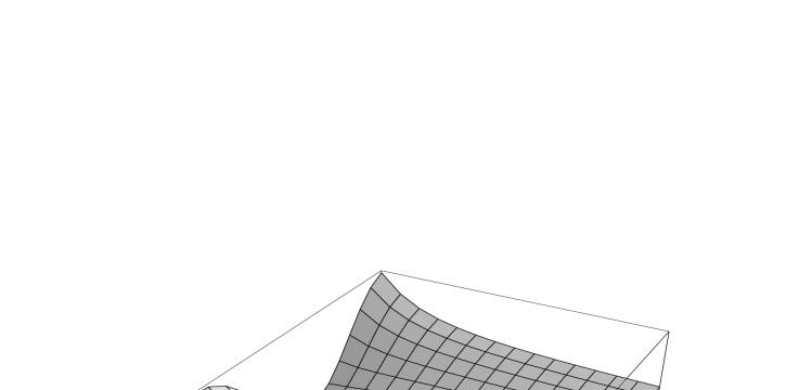
Figure 2:

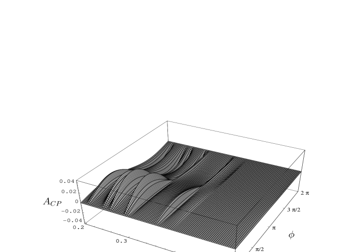
Figure 3:

References

[1] W. S. Hou, R. S. Willey and A. Soni,
Phys. Rev. Lett. 58, 1608 (1987).
[2] N. G. Deshpande and J. Trampetic,
Phys. Rev. Lett. 60, 2583 (1988).
[3] C. S. Kim, T. Morozumi and A. I. Sanda,
Phys. Lett. B 218, 343 (1989).
[4] B. Grinstein, M. J. Savage and M. B. Wise,
Nucl. Phys. B 319, 271 (1989).
[5] C. Dominguez, N. Paver and Riazuddin,
Phys. Lett. B 214, 459 (1988).
[6] N. G. Deshpande, J. Trampetic and K. Ponose,
Phys. Rev. D 39, 1461 (1989).
[7] P. J. O’Donnell and H. K. Tung,
Phys. Rev. D 43, 2067 (1991).
[8] N. Paver and Riazuddin,
Phys. Rev. D 45, 978 (1992).
[9] A. Ali, T. Mannel and T. Morozumi,
Phys. Lett. B 273, 505 (1991).
[10] A. Ali, G. F. Giudice and T. Mannel,
Z. Phys. C 67, 417 (1995).
[11] C. Greub, A. Ioannissian and D. Wyler,
Phys. Lett. B 346, 145 (1995);
D. Liu, Phys. Lett. B 346, 355 (1995);
G. Burdman, Phys. Rev. D 52, 6400 (1995);
Y. Okada, Y. Shimizu and M. Tanaka,
Phys.Lett. B 405, 297 (1997).
[12] A. J. Buras and M. Münz,
Phys. Rev. D 52, 186 (1995).
[13] N. G. Deshpande, X. -G. He and J. Trampetic,
Phys. Lett. B 367, 362 (1996).
[14] S. Bertolini, F. Borzumati, A. Masiero, G. Ridolfi,
Nucl.Phys. B 353, 591 (1991).
[15] F. Krüger and L. M. Sehgal
Phys. Rev. D 55,2799 (1997).
[16] F. Krüger and L. M. Sehgal
Phys. Rev. D 56, 5452 (1997).
[17] S. Glashow and S. Weinberg,
Phys. Rev. D 15, 1958 (1977).
[18] Talk by R. Briere, CLEO-CONF-98-17, ICHEP98-1011, in Proceedings of
ICHEP98, Vancouver, Canada, July 1998; and in talk by J. Alexander,
in Proceedings of ICHEP98, Vancouver, Canada, July 1998.
[19] R. Barate et al., ALEPH Collaboration,
Phys. Lett. B 429, 169 (1998).
[20] F. Borzumati and C. Greub,
Phys. Rev. D 58, 074004 (1998).
[21] M. Ciuchini, G. Degrassi, P. Gambino, G.F. Giudice,
Nucl.Phys. B 527, 21 (1998).
[22] T.P. Cheng and M. Sher,
Phys. Rev. D 35, 3484 (1987);
ibid. D 44, 1461 (1991);
W.S. Hou, Phys. Lett. B 296, 179 (1992);
A. Antaramian, L. Hall, and A. Rasin,
Phys. Rev. Lett. 69, 1871 (1992);
L. Hall and S. Weinberg, Phys. Rev D 48, 979 (1993);
M.J. Savage, Phys. Lett. B 266, 135 (1991).
[23] D. Atwood, L. Reina, and A. Soni,
Phys. Rev. D 55, 3156 (1997).
[24] T. M. Aliev and E. İltan,
Phys. Rev. D 58, 095014 (1998);
J. Phys. G 25, 989 (1999).
[25] L. Wolfenstein and Y.L. Wu,
Phys. Rev. Lett. 73, 2809 (1994).
[26] D. Bowser-Chao, K. Cheung, W.-Y. Keung,
Phys. Rev. D 59, 11506 (1999).
[27] T. M. Aliev and M. Savcı,
Phys. Lett. B 452, 318 (1999);
T. M. Aliev and M. Savcı,
Phys. Rev. D 60, 014005 (1999).
[28] G. Buchalla, A. Buras, and M. Lautenbacher,
Rev. Mod. Phys. 68, 1125 (1996).
[29] A.J. Buras, M. Misiak, Münz, and S. Pokorski,
Nucl. Phys. B 424, 374 (1994).
[30] B. Grinstein, R. Springer, and M. Wise,
Nucl. Phys. B 339, 269 (1990).
[31] M. Misiak,
Nucl. Phys. B 393, 23 (1993), Erratum, ibid. B 439, 461 (1995);
A. J. Buras and M. Münz,
Phys. Rev. D 52, 186 (1995).
[32] A. I. Vainshtein, V. I. Zakharov, L. B. Okun and
M. A. Shifman,
Sov. J. Nucl. Phys. 24, 427 (1976).
[33] T. Mannel, W. Roberts, Z. Ryzak,
Nucl. Phys. B 355, 38 (1991).
[34] Chao–Shang Huang and Huang–Gang Yan,
Phys. Rev. D 59, 114022 (1999).
[35] J. Kalinowski,
Phys. Lett. B 245, 201 (1990).
[36] A. K. Grant,
Phys. Rev. D 51, 207 (1995).