Status of the MSW Solutions of the Solar Neutrino Problem

Abstract

We present an updated global analysis of two-flavor MSW solutions to the solar neutrino problem. We perform a fit to the full data set corresponding to the 825-day Super–Kamiokande data sample as well as to Chlorine, GALLEX and SAGE experiments. In our analysis we use all measured total event rates as well as all Super–Kamiokande data on the zenith angle dependence, energy spectrum and seasonal variation of the events. We compare the quality of the solutions of the solar neutrino anomaly in terms of conversions of $\nu_{e}$ into active or sterile neutrinos. For the case of conversions into active neutrinos we find that, although the data on the total event rates favours the Small Mixing Angle (SMA) solution, once the full data set is included both SMA and Large Mixing Angle (LMA) solutions give an equally good fit to the data. We find that the best–fit points for the combined analysis are $\Delta m^{2}=3.6\times 10^{-5}$ eV² and $\sin^{2}2\theta=0.79$ with $\chi^{2}_{min}=35.4/30$ d. o. f and $\Delta m^{2}=5.1~{}\times 10^{-6}$ eV² and $\sin^{2}2\theta=5.5\times 10^{-3}$ with $\chi^{2}_{min}=37.4/30$ d. o. f. In contrast with the earlier 504-day study of Bahcall-Krastev-Smirnov our results indicate that the LMA solution is not only allowed, but slightly preferred. On the other hand we show that seasonal effects, although small, may still reach 11% in the lower part of the LMA region, without conflict with the negative hints of a day-night variation (6% is due to the eccentricity of the Earth’s orbit). In particular the best-fit LMA solution predicts a seasonal effect of 8.5%. For conversions into sterile neutrinos only the SMA solution is possible with best–fit point $\Delta m^{2}=5.0~{}\times 10^{-6}$ eV² and $\sin^{2}2\theta=3.\times 10^{-3}$ and $\chi^{2}_{min}=40.2/30$ d. o. f. We also consider departures of the Standard Solar Model (SSM) of Bahcall and Pinsonneault 1998 (BP98) by allowing arbitrary ${}^{8}B$ and $hep$ fluxes. These modifications do not alter significantly the oscillation parameters. The best fit is obtained for ${}^{8}B/^{8}B_{SSM}=0.61$ and $hep/hep_{SSM}=12$ for the SMA solution both for conversions into active or sterile neutrinos and ${}^{8}B/^{8}B_{SSM}=1.37$ and $hep/hep_{SSM}=38$ for the LMA solution.

I Introduction

It is already three decades since the first detection of solar neutrinos. It was realized from the very beginning that the observed rate at the Homestake experiment [1] was far lower than the theoretical expectation based on the standard solar model [2] with the implicit assumption that neutrinos created in the solar interior reach the earth unchanged, i.e. they are massless and have only standard properties and interactions. In the first two decades of solar neutrino research, the problem consisted only of the discrepancy between theoretical expectations based upon solar model calculations and the observations of the capture rate in the chlorine solar neutrino experiment. This discrepancy led to a change in the original goal of using solar neutrinos to probe the properties of the solar interior towards the study of the properties of the neutrino itself.

From the experimental point of view much progress has been done in recent years. We now have available the results of five experiments, the original Chlorine experiment at Homestake [3], the radio chemical Gallium experiments on pp neutrinos, GALLEX [4] and SAGE [5], and the water Cherenkov detectors Kamiokande [6] and Super–Kamiokande [7, 8]. The latter has been able not only to confirm the original detection of solar neutrinos at lower rates than predicted by standard solar models, but also to demonstrate directly that the neutrinos come from the sun by showing that recoil electrons are scattered in the direction along the sun-earth axis. We now have good information on the time dependence of the event rates during the day and night, as well as a measurement of the recoil electron energy spectrum. After 825 days of operation, Super–Kamiokande has also presented preliminary results on the seasonal variation of the neutrino event rates, an issue which will become important in discriminating the MSW scenario from the possibility of neutrino oscillations in vacuum [9, 10].

On the other hand there has been improvement on solar modelling and nuclear cross sections. For example, helioseismological observations have now established that diffusion is occurring and by now most solar models incorporate the effects of helium and heavy element diffusion [11, 12]. The quality of the experiments themselves and the robustness of the theory make us confident that in order to describe the data one must depart from the Standard Model (SM) of particle physics interactions, by endowing neutrinos with new properties. In theories beyond the Standard Model of particle physics neutrinos may naturally have exotic properties such as non-orthonormality [13], flavour-changing interactions [14], transition magnetic moments  [15] and neutrino decays [16], the most generic is the existence of mass. While many of these may play a role in neutrino propagation and therefore in the explanation of the data [17] it is undeniable that the most generic and popular explanation of the solar neutrino anomaly is in terms of neutrino masses and mixing leading to neutrino oscillations either in vacuum [18] or via the matter-enhanced MSW mechanism [19].

In this paper we study the implications of the present data on solar neutrinos in the framework of the two-flavor MSW solutions to the solar neutrino problem. We perform a global fit to the full data set corresponding to 825 days of data of the Super–Kamiokande experiment as well as to Chlorine, GALLEX and SAGE. In our analysis we use as SSM the latest results from the most accurate calculation of neutrino fluxes by Bahcall and Pinsonneault [20] which incorporates the new normalization for the low energy cross section $S_{17}=19^{+4}_{-2}~{}{\rm eV~{}b}$ indicated by the recent studies at the Institute of Nuclear Theory [21]. We have also considered the possibility of departing from the SSM of BP98 by allowing a free normalization of the ${}^{8}B$ flux and $hep$ neutrino fluxes and we present the results we obtain when we treat these normalization as free parameters.

We combined the measured total event rates at Chlorine, Gallium and Super–Kamiokande experiments with the Super–Kamiokande data on the zenith angle dependence, energy spectrum and seasonal variation of the events. The goal of such analysis is not only to compare the quality of the solutions to the solar neutrino anomaly in terms of flavour oscillations of $\nu_{e}$ into active or sterile neutrinos but also to study the weight of different observables on the determination of the underlying neutrino physics parameters as emphasized in Ref. [22]. The outline of the paper is as follows. In Sec. II we present the basic elements that enter into our calculation of the observables and the definitions used in the statistical combination of the data. Section III contains our results of the allowed (or excluded) regions of oscillation parameters from the analyses of the different observables. The results on the allowed regions from the combined analysis of the total event rates is contained in Sec. III A. The constraints arising from the Super–Kamiokande searches for day–night variation of the event rates are discussed in Sec. III B. In Sec. III C we discuss the information which can be extracted from the distortion of the recoil electron energy spectrum measured by Super–Kamiokande. The restrictions arising from the preliminary Super–Kamiokande data on the seasonal variation of the event rates are studied in Sec. III D. In Sec. III E we present our results from the global fit to the full data set and we determine the allowed range of oscillation parameters which are consistent with all the data. Finally in Sec. IV we discuss the possible implications of our results for future investigations.

Our results show that for oscillation into active neutrinos although the data on the total event rates favours the SMA angle solution, once the full data set is included both SMA and LMA give an equally good fit to the data. We find that the best–fit points for the combined analysis are $\Delta m^{2}=3.6\times 10^{-5}$ eV² and $\sin^{2}2\theta=0.79$ with $\chi^{2}_{min}=35.4/30$ d. o. f. and $\Delta m^{2}=5.1\times 10^{-6}$ eV² and $\sin^{2}2\theta=5.5\times 10^{-3}$ with $\chi^{2}_{min}=37.4/30$ d. o. f. We note that in contrast with the earlier 504-day study of Ref. [22] our results indicate that the LMA solution is not only allowed, but actually slightly preferred. The existence of hints that the LMA MSW solution could be correct was also discussed in Ref.[23]. On the other hand we find good quantitative agreement with the recent results of [8] as well as qualitative agreement with the old results of [24] based on a smaller sample. We show that seasonal effects may be no-negligible in the lower part of the LMA region, without conflict with the negative hints of a day-night variation. In particular the best-fit LMA solution predicts a seasonal effect of 8.5%, 6% of which is due to the eccentricity of the Earth’s orbit. For conversions into sterile neutrinos we find that only the SMA solution is possible with best–fit point $\Delta m^{2}=5.0\times 10^{-6}$ eV² and $\sin^{2}2\theta=3.0\times 10^{-3}$ and $\chi^{2}_{min}=40.2/30$ d. o. f. We also consider departures of the Standard Solar Model (SSM) of Bahcall and Pinsonneault 1998 (BP98) by allowing arbitrary ${}^{8}B$ and $hep$ fluxes. These modifications do not affect significantly the oscillation parameters. We find that the best fit is obtained for ${}^{8}B/^{8}B_{SSM}=0.61$ and $hep/hep_{SSM}=12$ for the SMA solution both for conversions into active or sterile neutrinos and ${}^{8}B/^{8}B_{SSM}=1.37$ and $hep/hep_{SSM}=38$ for the LMA solution.

II Data and Techniques

In order to study the possible values of neutrino masses and mixing for the MSW solution to the solar neutrino problem, we have used data on the total event rates measured at the Chlorine experiment in Homestake [3], at the two Gallium experiments GALLEX and SAGE [4, 5] and at the water Cerenkov detector Super–Kamiokande. Apart from total event rates we have in this case the zenith angle distribution of the events, the electron recoil energy spectrum and the seasonal distribution of events, all measured with their recent 825-day data sample [8].

We first describe our calculation of the different observables. For simplicity we consider the two-neutrino mixing case

$$\nu_{e}=\cos\theta~{}\nu_{1}+\sin\theta~{}\nu_{2}\;,\;\nu_{x}=-\sin\theta~{}\nu_{1}+\cos\theta~{}\nu_{2}~{},$$ (1)

where $x$ can label either an active, $x=\mu,\tau$, or sterile neutrino, $x=s$. In order to account for Earth regeneration effects, we have determined the solar neutrino survival probability $P_{ee}$ in the usual way, assuming that the neutrino state arriving at the Earth is an incoherent mixture of the $\nu_{1}$ and $\nu_{2}$ mass eigenstates.

$$P_{ee}=P_{e1}^{Sun}P_{1e}^{Earth}+P_{e2}^{Sun}P_{2e}^{Earth}$$ (2)

where $P_{e1}^{Sun}$ is the probability that a solar neutrino, that is created as $\nu_{e}$, leaves the Sun as a mass eigenstate $\nu_{1}$, and $P_{1e}^{Earth}$ is the probability that a neutrino which enters the Earth as $\nu_{1}$ arrives at the detector as $\nu_{e}$. Similar definitions apply to $P_{e2}^{Sun}$ and $P_{2e}^{Earth}$.

The quantity $P_{e1}^{Sun}$ is given, after discarding the fast oscillating terms, as

$$P_{e1}^{Sun}=1-P_{e2}^{Sun}=\frac{1}{2}+(\frac{1}{2}-P_{LZ})cos[2\theta_{m}(t_{0})]$$ (3)

where $P_{LZ}$ denotes the improved Landau-Zener probability [25] and $\theta(t_{0})_{m}$ is the mixing angle in matter at the neutrino production point. In our calculations of the expected event rates we have averaged this probability with respect to the production point. The electron and neutron number density in the sun and the production point distribution were taken from Ref. [26].

In order to obtain the conversion probabilities in the Earth, $P_{ie}^{Earth}$, we integrate the evolution equation in matter assuming a step function profile of the Earth matter density (the Earth as consisting of mantle and core of constant densities equal to the corresponding average densities, $\bar{\rho}_{m}\simeq 4.5$ $g/cm^{3}$ and $\bar{\rho}_{c}\simeq 11.5$ $g/cm^{3}$). To convert from the mass density to electron and neutron number density we use the charge to nucleon ratio $Z/A=0.497$ for the mantle and $Z/A=0.467$ for the core. In the notation of Ref. [27], we obtain for $P_{2e}^{Earth}=1-P_{1e}^{Earth}$

$$P_{2e}^{Earth}(\Phi)=(Zsin\theta)^{2}+(W_{1}cos\theta+W_{3}sin\theta)^{2}\\$$ (4)

where $\theta$ is the mixing angle in vacuum and the Earth matter effect is included in the formulas for $Z,W_{1}$ and $W_{3}$, which can be found in Ref. [27]. $P_{2e}^{Earth}$ depends on the amount of Earth matter travelled by the neutrino on its way to the detector, or, in other words, on its arrival direction which is usually parametrized in terms of the nadir angle, $\Phi$, of the sun at the detector site. Due to this effect the survival probability is, in general, time dependent. This Earth regeneration effect is important in the study of the zenith angle distribution of events as well as in their seasonal variation [9, 28].

A Rates

Here we update previous analyses of solar neutrino data [22, 24] by including the recent 825-day Super–Kamiokande data sample. We perform a dedicated analysis of the seasonal variation data and we anticipate its future role in discriminating between different solutions of the solar neutrino anomaly. Working in the context of the BP98 standard solar model of Ref. [20] we also allow for a free normalization of the ${}^{8}B$ flux and of the hep flux. In our statistical treatment of the data we follow closely the analysis of Ref. [29] with the updated uncertanties given in Refs. [20, 26].

In our study we use the measured rates shown in Table I. For the combined fit we adopt the $\chi^{2}$ definition:

$$\chi^{2}_{R}=\sum_{i,j=1,3}(R^{th}_{i}-R^{exp}_{i})\sigma_{ij}^{-2}(R^{th}_{j}-R^{exp}_{j})$$ (5)

where $R^{th}_{i}$ is the theoretical prediction of the event rate in detector $i$ and $R^{exp}_{i}$ is the measured rate. The error matrix $\sigma_{ij}$ contains not only the theoretical uncertainties but also the experimental errors, both systematic and statistical.

The general expression of the expected event rate in the presence of oscillations in experiment $i$ is given by $R^{th}_{i}$ :

$$R^{th}_{i} = \sum_{k=1,8}\phi_{k}\int\!dE_{\nu}\,\lambda_{k}(E_{\nu})\times\big{[}\sigma_{e,i}(E_{\nu})\langle P_{ee}(E_{\nu},t)\rangle$$ (7)

$$+\sigma_{x,i}(E_{\nu})(1-\langle P_{ee}(E_{\nu},t)\rangle)\big{]},$$

where $E_{\nu}$ is the neutrino energy, $\phi_{k}$ is the total neutrino flux and $\lambda_{k}$ is the neutrino energy spectrum (normalized to 1) from the solar nuclear reaction $k$  [30] with the normalization given in Ref. [20]. Here $\sigma_{e,i}$ ($\sigma_{x,i}$) is the $\nu_{e}$ ($\nu_{x}$, $x=\mu,\,\tau$) interaction cross section in the Standard Model [31] with the target corresponding to experiment $i$, and $\langle P_{ee}(E_{\nu},t)\rangle$ is the time–averaged $\nu_{e}$ survival probability.

For the Chlorine and Gallium experiments we use improved cross sections $\sigma_{\alpha,i}(E)$ $(\alpha=e,\,x)$ from Ref. [26]. For the Super–Kamiokande experiment we calculate the expected signal with the corrected cross section given in Sec. II C.

The expected signal in the absence of oscillations, $R^{\rm BP98}_{i}$, can be obtained from Eq.(7) by substituting $P_{ee}=1$. In Table I we also give the expected rates at the different experiments which we obtain using the fluxes of Ref. [20].

B Day-Night Variation

As already mentioned, in the MSW picture the expected event rates can be different when the neutrinos travel through the Earth due to the $\nu_{e}$ regeneration effect [28]. As a result in certain regions of the oscillation parameters the expected event rates depend on the zenith angle of the sun as observed from the experiment site, since this determines the amount of Earth matter crossed by the neutrino on its way to the detector.

The Super–Kamiokande Collaboration has studied the dependence of the event rates with the period of time along the day and the night. They present their results in the form of a zenith angle distribution of events.

In our analysis we have used the experimental results from the Super–Kamiokande Collaboration on the zenith angle distribution of events taken on 5 night periods and the day averaged value, shown in Table II which we graphically reduced from Ref. [8]

We define $\chi^{2}$ for the zenith angle data as:

$$\chi^{2}_{Z}=\sum_{i=1,6}\frac{(\alpha_{z}\frac{\displaystyle R^{th}_{i}}{\displaystyle R^{\rm BP98}_{i}}-R^{exp}_{i})^{2}}{\sigma_{i}^{2}}$$ (8)

where we have neglected the possible correlation between the errors of the different angular bins which could arise from systematical uncertainties. The factor $\alpha_{z}$ is included in order to avoid over-counting the data on the total event rate which is already included in $\chi^{2}_{R}$.

We compute the expected event rate in the period $i$ in the presence of oscillations as,

$$R^{th}_{i} = \frac{\displaystyle 1}{\displaystyle\Delta\tau_{i}}\int_{\tau(cos\Phi_{min,i})}^{\tau(cos\Phi_{max,i})}d\tau\sum_{k=1,8}\phi_{k}\int\!dE_{\nu}\,\lambda_{k}(E_{\nu})\times\big{[}\sigma_{e,i}(E_{\nu})\langle P_{ee}(E_{\nu},\tau)\rangle$$ (10)

$$+\sigma_{x,i}(E_{\nu})(1-\langle P_{ee}(E_{\nu},\tau)\rangle)\big{]}$$

where $\tau$ measures the yearly averaged length of the period $i$ normalized to 1, so $\Delta\tau_{i}=\tau(cos\Phi_{max,i})-\tau(cos\Phi_{min,i})=$ .500, .086, .091, .113, .111, .099 for the day and five night periods respectively.

Super–Kamiokande has also presented their results on the day-night variation in the form of a day-night asymmetry,

$$A_{D/N}=\frac{Day-Night}{Day+Night}=-0.065\pm 0.031\mbox{(stat.)}\pm 0.013\mbox{(syst.)}$$ (11)

Since the information included in the zenith angle dependence already contains the day-night asymmetry, we have not added the asymmetry as an independent observable in our fit. Notice also, that being a ratio of event rates, the asymmetry is not a Gaussian-distributed observable and therefore should not be included in a $\chi^{2}$ analysis.

C Recoil Electron Spectrum

The Super-Kamiokande Collaboration has also measured the recoil electron energy spectrum. In their published analysis [32] after 504 days of operation they present their results for energies above 6.5 MeV using the Low Energy (LE) analysis in which the recoil energy spectrum is divided into 16 bins, 15 bins of 0.5 MeV energy width and the last bin containing all events with energy in the range 14 MeV to 20 MeV. Below 6.5 MeV the background of the LE analysis increases very fast as the energy decreases. Super–Kamiokande has designed a new Super Low Energy (SLE) analysis in order to reject this background more efficiently so as to be able to lower their threshold down to 5.5 MeV. In their 825-day data [8] they have used the SLE method and they present results for two additional bins with energies between 5.5 MeV and 6.5 MeV.

In our study we use the experimental results from the Super–Kamiokande Collaboration on the recoil electron spectrum on the 18 energy bins including the results from the LE analysis for the 16 bins above 6.5 MeV and the results from the SLE analysis for the two low energy bins below 6.5 MeV, shown in Table III.

Notice that in Table III we have symmetrized the errors to be included in our $\chi^{2}$ analysis. We have explicitly checked that the exclusion region is very insensitive to this symmetrization. We define $\chi^{2}$ for the spectrum as

$$\chi^{2}_{S}=\sum_{i,j=1,18}(\alpha_{sp}\frac{\displaystyle R^{th}_{i}}{R^{\rm BP98}_{i}}-R^{exp}_{i})\sigma_{ij}^{-2}(\alpha_{sp}\frac{\displaystyle R^{th}_{j}}{R^{\rm BP98}_{i}}-R^{exp}_{j})$$ (12)

where

$$\sigma^{2}_{ij}=\delta_{ij}(\sigma^{2}_{i,stat}+\sigma^{2}_{i,uncorr})+\sigma_{i,exp}\sigma_{j,exp}+\sigma_{i,cal}\sigma_{j,cal}$$ (13)

Again, we introduce a normalization factor $\alpha_{sp}$ in order to avoid double-counting with the data on the total event rate which is already included in $\chi^{2}_{R}$. Notice that in our definition of $\chi^{2}_{S}$ we introduce the correlations amongst the different systematic errors in the form of a non-diagonal error matrix in analogy to our previous analysis of the total rates. These correlations take into account the systematic uncertainties related to the absolute energy scale and energy resolution, which were not yet available at the time the analysis of Ref. [22] was performed. Note that our procedure is different from that used by the Super-Kamiokande collaboration. However we will see in Sec. III C that both methods give very similar results for the exclusion regions. This provides a good test of the robustness of the results of the fits, in the sense that they do not depend on the details of the statistical analysis.

The general expression of the expected rate in the presence of oscillations $R^{th}$ in a bin, is given from Eq.(7) but integrating within the corresponding electron recoil energy bin and taking into account that the finite energy resolution implies that the measured kinetic energy $T$ of the scattered electron is distributed around the true kinetic energy $T^{\prime}$ according to a resolution function $Res(T,\,T^{\prime})$ of the form [33]:

$$Res(T,\,T^{\prime})=\frac{1}{\sqrt{2\pi}s}\exp\left[{-\frac{(T-T^{\prime})^{2}}{2s^{2}}}\right]\ ,$$ (14)

where

$$s=s_{0}\sqrt{T^{\prime}/{\rm MeV}}\ ,$$ (15)

and $s_{0}=0.47$ MeV for Super–Kamiokande [7, 34]. On the other hand, the distribution of the true kinetic energy $T^{\prime}$ for an interacting neutrino of energy $E_{\nu}$ is dictated by the differential cross section $d\sigma_{\alpha}(E_{\nu},\,T^{\prime})/dT^{\prime}$, that we take from [31]. The kinematic limits are:

$$0\leq T^{\prime}\leq{\overline{T}}^{\prime}(E_{\nu})\ ,\ \ {\overline{T}}^{\prime}(E_{\nu})=\frac{E_{\nu}}{1+m_{e}/2E_{\nu}}\ .$$ (16)

For assigned values of $s_{0}$, $T_{\rm min}$, and $T_{\rm max}$, the corrected cross section $\sigma_{\alpha}(E)$ $(\alpha=e,\,x)$ is given as

$$\sigma_{\alpha}(E_{\nu})=\int_{T_{\rm min}}^{T_{\rm max}}\!dT\int_{0}^{{\overline{T}}^{\prime}(E_{\nu})}\!dT^{\prime}\,Res(T,\,T^{\prime})\,\frac{d\sigma_{\alpha}(E_{\nu},\,T^{\prime})}{dT^{\prime}}\ .$$ (17)

In Fig. III we show our results for the recoil electron spectrum in the absence of oscillations and compare it with the expectations from the Super–Kamiokande Monte-Carlo. We see that the agreement is excellent. In this figure no normalization has been included.

D Seasonal Variation

After 825 days of operation, Super–Kamiokande has also presented preliminary results on the seasonal variation of the neutrino event rates [8] which seem to hint at a seasonal variation of the data, especially for recoil electron energies above 11.5 MeV (see Table  IV). As discussed in Ref. [9, 10] the expected MSW event rates do exhibit a seasonal effect. In the LMA region such dependence can be expected mainly due to the different night duration throughout the year at the experimental site and also due to the different averaged Earth densities crossed by the neutrino during the night periods, which lead to a seasonal-dependent $\nu_{e}$ regeneration effect in the Earth. On the other hand, in the SMA region, Earth matter effects are due to resonant conversion of neutrinos in the Earth which is only possible when neutrinos travel both through the mantle and the core [28]. Thus we find that in the SMA region the seasonal variation is associated with the fact that at Super–Kamiokande site only in October-March nights there are neutrinos arriving at sufficiently low zenith angle to satisfy the resonant condition.

We define $\chi^{2}$ for the seasonal variation data as,

$$\chi^{2}_{Sea}=\sum_{i=1,8}\frac{(\alpha_{sea}\frac{\displaystyle R^{th}_{i}}{R^{\rm BP98}_{i}\displaystyle}-R^{exp}_{i})^{2}}{\sigma_{i}^{2}}$$ (18)

where, as before, the normalization factor $\alpha_{sea}$ is introduced to avoid double-counting.

Taking into account the relative position of the Super–Kamiokande setup in each period of the year, we calculate the distribution of the events as

$$\frac{R^{th}_{i}(t_{i},\Delta t)}{R^{\rm BP98}_{i}(\Delta t)}=\frac{\displaystyle\int_{t_{i}-\Delta t/2}^{t_{i}+\Delta t/2}dt\,R^{th}(t)}{\displaystyle\Delta tR^{th}(t)}$$ (19)

Here $\Delta t=1.5$ months and $R^{th}(t)$ is obtained from Eq.(7) but using the time–dependent survival probabilities and integrating the recoil electron energy above 11.5 MeV. Notice that, unlike in the 708 days data sample, in order to compare our results with the recent data on the seasonal dependence of the event rates from the Super–Kamiokande Collaboration for the 825 data sample, we have not included the geometrical seasonal neutrino flux variation due to the variation of the Sun-Earth distance arising from the Earth’s orbit eccentricity because the new Super–Kamiokande data is already corrected for this geometrical variation.

III Fits: Results

We now turn to the results of our fits with the observables described above. We have obtained the regions of allowed oscillation parameters $\Delta m^{2}$-$\sin^{2}2\theta$ by obtaining the minimum $\chi^{2}$ and imposing the condition $\chi^{2}\leq\chi^{2}_{min}$+$\Delta\chi^{2}(2,CL)$ where $\Delta\chi^{2}(2,CL)=4.61(9.21)$ for 90% (99%) CL regions.

A Rates

We first determine the allowed range of oscillation parameters using only the total event rates of the Chlorine, Gallium and Super–Kamiokande experiments. The average event rates for these experiments are summarized in Table I. We have not included in our analysis the Kamiokande data [6] as it is well in agreement with the results from the Super–Kamiokande experiment and the precision of this last one is much higher [8]. For the Gallium experiments we have used the weighted average of the results from GALLEX [4] and SAGE [5] detectors.

Using the predicted fluxes from the BP98 model the $\chi^{2}$ for the total event rates is $\chi^{2}_{SSM}=62.4$ for 3 d. o. f. This means that the SSM together with the SM of particle interactions can explain the observed data with a probability lower than $10^{-12}$!

In the case of active-active neutrino oscillations we find that the best–fit point is obtained for the SMA solution with

$$\Delta m^{2} = 5.6\times 10^{-6}\mbox{eV}^{2}\;,$$ (20)

$$\sin^{2}2\theta = 6.3\times 10^{-3}\;,$$ (21)

$$\chi^{2}_{min} = 0.37\;,$$ (22)

what implies that the solution is acceptable with a 55% CL.

There are two more local minima of $\chi^{2}$. One is the LMA solution with the best fit for

$$\Delta m^{2} = 1.4\times 10^{-5}\mbox{eV}^{2}\;,$$ (23)

$$\sin^{2}2\theta = 0.67\;,$$ (24)

$$\chi^{2}_{min} = 2.92\;,$$ (25)

which is acceptable with at 91% CL. The other is the LOW solution with best–fit point

$$\Delta m^{2} = 1.3\times 10^{-7}\mbox{eV}^{2}\;,$$ (26)

$$\sin^{2}2\theta = 0.94\;,$$ (27)

$$\chi^{2}_{min} = 7.4\;,$$ (28)

which is only acceptable at 99% CL.

In the case of active-sterile neutrino oscillations the best–fit point is obtained for the SMA solution with

$$\Delta m^{2} = 5.0\times 10^{-6}\mbox{eV}^{2}\;,$$ (29)

$$\sin^{2}2\theta = 5.0\times 10^{-3}\;,$$ (30)

$$\chi^{2}_{min} = 2.6\;,$$ (31)

acceptable at 90% CL. The LMA and LOW solutions are not acceptable for oscillation into sterile neutrinos. In those regions $\chi^{2}_{min}\geq 19.5$ implying that they are excluded at the 99.999% CL. Unlike active neutrinos which lead to events in the Super–Kamiokande detector by interacting via neutral current with the electrons, sterile neutrinos do not contribute to the Super–Kamiokande event rates. Therefore a larger survival probability for ${}^{8}B$ neutrinos is needed to accommodate the measured rate. As a consequence a larger contribution from ${}^{8}B$ neutrinos to the Chlorine and Gallium experiments is expected, so that the small measured rate in Chlorine can only be accommodated if no ${}^{7}Be$ neutrinos are present in the flux. This is only possible in the SMA solution region, since in the LMA and LOW regions the suppression of ${}^{7}Be$ neutrinos is not enough.

In Fig. 2 we show the 90% and 99% CL allowed regions in the plane $\Delta m^{2}$-$\sin^{2}2\theta$. The best–fit points in each region are marked. We find that as far as the analysis of the total rates is concerned, there is no substantial change in the best–fit points in the three regions as compared to the previous most recent analysis including the 504 days of Super–Kamiokande data [22].

We have also considered the possibility of departing from the SSM of BP98 by allowing a free normalization of the ${}^{8}B$ flux and we treat this normalization as a free parameter $\beta$ in our analysis. Figure 3 shows the allowed regions in the MSW parameter space when $\beta$ is allowed to take arbitrary values. The best fit SMA solution is obtained for

$$\Delta m^{2} = 5.0\times 10^{-6}\mbox{eV}^{2}\;,$$ (32)

$$\sin^{2}2\theta = 5.0\times 10^{-3}\;,$$ (33)

$$\beta = 0.82$$ (34)

$$\chi^{2}_{min} = 0.05\;.$$ (35)

The best fit for the LMA solution occurs at:

$$\Delta m^{2} = 1.6\times 10^{-5}\mbox{eV}^{2}\;,$$ (36)

$$\sin^{2}2\theta = 0.63\;,$$ (37)

$$\beta = 1.32$$ (38)

$$\chi^{2}_{min} = 0.47\;,$$ (39)

and the LOW solution has its best–fit point at $\beta=.98$ and therefore coincides with the one obtained in Eq.(27).

In the case of active-sterile neutrino oscillations the best–fit point is obtained for the SMA solution :

$$\Delta m^{2} = 5.0\times 10^{-6}\mbox{eV}^{2}\;,$$ (40)

$$\sin^{2}2\theta = 3.2\times 10^{-3}\;,$$ (41)

$$\beta = 0.75$$ (42)

$$\chi^{2}_{min} = 2.16\;.$$ (43)

For all solutions we find that the main effect of considering a free normalization of the ${}^{8}B$ flux is upon the quality of the fits, as measured by the depth of the $\chi^{2}$. Next comes the position of the best–fit points, mainly a reduction in the value of the mixing angle. The allowed regions are considerably enlarged as can be seen by comparing Figs. 2 and 3.

B Yearly Averaged Zenith Angle Dependence

We now study the constraints on the oscillation parameters from the Super–Kamiokande Collaboration measurement of the zenith angle distribution of events. We use the data taken on 5 night periods and the day averaged value shown in Table II which we graphically reduced from Ref. [8].

Considering only the zenith angle data (not including the information from the total rates), the best–fit point in the case of active-active neutrino oscillations is obtained for $\Delta m^{2}=4.5\times 10^{-5}$ eV² and $\sin^{2}2\theta=1.0$ with $\chi^{2}_{min}=2.3$ for 3 d. o. f. and in the case of active-sterile neutrino oscillations is obtained for $\Delta m^{2}=3.2\times 10^{-5}$ eV² and $\sin^{2}2\theta=.98$ with $\chi^{2}_{min}=2.2$. With these values we calculate the excluded region of parameters at the 99% CL, shown in Fig 4. Notice that the zenith angle data favours the LMA solution of the solar neutrino problem.

When combining the information from both total rates and zenith angle data, we obtain that in the case of active-active neutrino oscillations the best–fit point is still obtained for the SMA solution with

$$\Delta m^{2} = 5.0\times 10^{-6}\mbox{eV}^{2}\;,$$ (44)

$$\sin^{2}2\theta = 6.3\times 10^{-3}\;,$$ (45)

$$\chi^{2}_{min} = 5.9\;,$$ (46)

for 6 d. o. f. which is acceptable with a 56% CL. However the LMA solution becomes relatively better with a local minimum at

$$\Delta m^{2} = 4.5\times 10^{-5}\mbox{eV}^{2}\;,$$ (47)

$$\sin^{2}2\theta = 0.80\;,$$ (48)

$$\chi^{2}_{min} = 7.2\;,$$ (49)

valid at 70% CL. This difference arises from the fact that, although small, some effect is observed in the zenith angle dependence which points towards a larger event rate during the night than during the day, and that this difference is constant during the night as expected for the LMA solution [23]. In the SMA solution, however, the enhancement is expected to occur mainly in the fifth night [28].

The LOW solution is almost un–modified and presents the best–fit point at

$$\Delta m^{2} = 1.0\times 10^{-7}\mbox{eV}^{2}\;,$$ (50)

$$\sin^{2}2\theta = 0.94\;,$$ (51)

$$\chi^{2}_{min} = 12.7\;,$$ (52)

which is acceptable at 95% CL.

In the case of active-sterile neutrino oscillations the best–fit point is obtained for the SMA solution with

$$\Delta m^{2} = 5.0\times 10^{-6}\mbox{eV}^{2}\;,$$ (53)

$$\sin^{2}2\theta = 5.0\times 10^{-3}\;,$$ (54)

$$\chi^{2}_{min} = 8.1\;,$$ (55)

valid at 77% CL.

Figure 4 shows the regions excluded at 99% CL by the zenith angle data alone, together with the 90% and 99% CL allowed regions in the plane $\Delta m^{2}$-$\sin^{2}2\theta$ from the combined analysis of rates plus zenith angle data. The best–fit points in each region are indicated. The main difference with respect to Fig. 2 is observed in the LMA allowed region which is cut from below, as the expected day-night variation is too large for smaller neutrino mass differences.

C Recoil Electron Spectrum

We now present the results of the study of the recoil electron spectrum data observed in Super–Kamiokande. Using the method described in Sec. II C we obtain that the $\chi^{2}$ for the undistorted energy spectrum (Standard Model case) is 20.1 for 17 d. o. f.. This corresponds to an agreement of the measured with the expected energy shape at the 27% CL. This value depends on the degree of correlation allowed between the different errors. In this way, reducing the correlation in the error matrix the agreement decreases down to 13%. This suggests that the correlations amongst the different systematic uncertainties related to the energy resolution will play an important role in the analysis of the energy spectrum. Indeed in our definition of $\chi^{2}_{S}$ we introduce the correlations amongst the different systematic errors in the form of a non-diagonal error matrix in analogy to our previous analysis of the total rates. These correlations take into account the systematic uncertainties related to the energy resolution. We believe that these might constitute the main difference between our treatment of the spectrum data and the earlier one presented in Ref. [22], when this experimental information was still unavailable.

We find that the best fit to the spectrum in the MSW plane for the case of active-active neutrino oscillations is obtained for $\Delta m^{2}=6.3\times 10^{-6}$ eV² and $\sin^{2}2\theta=0.08$ with $\chi^{2}_{min}=17.9$. For the case of active-sterile neutrino oscillations we get $\Delta m^{2}=6.3\times 10^{-6}$ eV² and $\sin^{2}2\theta=.08$ with $\chi^{2}_{min}=17$. With these values we obtain the excluded region of parameters at the 99% CL shown in Fig. 5.

We see that our results for the exclusion regions are quantitatively very similar to those of the Super-Kamiokande collaboration [8], even though our procedure is different from theirs. This provides a good test of the robustness of the results of the fit of the spectrum, in the sense that they do not depend on the details of the statistical analysis. In contrast we note that our results are different from those of Ref. [22].

When combining the information from both total rates and the recoil energy spectrum data we obtain that in the case of active-active neutrino oscillations both SMA and LMA solutions lead to fits to the data if similar quality. In this way, the best–fit for the LMA solution is

$$\Delta m^{2} = 1.4\times 10^{-5}\mbox{eV}^{2}\;,$$ (56)

$$\sin^{2}2\theta = 0.67\;,$$ (57)

$$\chi^{2}_{min} = 22.5\;,$$ (58)

while for the SMA solution we find

$$\Delta m^{2} = 5.6\times 10^{-6}\mbox{eV}^{2}\;,$$ (59)

$$\sin^{2}2\theta = 5.0\times 10^{-3}\;,$$ (60)

$$\chi^{2}_{min} = 23.4\;,$$ (61)

for 18. d. o. f. which are acceptable at  83%. Finally for the LOW solution we find

$$\Delta m^{2} = 1.0\times 10^{-7}\mbox{eV}^{2}\;,$$ (62)

$$\sin^{2}2\theta = 0.94\;,$$ (63)

$$\chi^{2}_{min} = 26.7\;,$$ (64)

with agreement with data only at the 8.5% CL.

In the case of active-sterile neutrino oscillations the best–fit point is obtained for the SMA solution with

$$\Delta m^{2} = 5.0\times 10^{-6}\mbox{eV}^{2}\;,$$ (65)

$$\sin^{2}2\theta = 3.0\times 10^{-3}\;,$$ (66)

$$\chi^{2}_{min} = 26.3\;.$$ (67)

acceptable at  90%.

In Fig. 5 we plot the excluded region at 99% CL by the energy spectrum data together with the 90% and 99% CL allowed regions in the plane $\Delta m^{2}$-$\sin^{2}2\theta$ from the combined analysis. The best–fit points in each region are marked.

The main point here is that the oscillation hypothesis does not improve considerably the fit to the energy spectrum as compared to the no-oscillation hypothesis. In this connection it has been suggested [35] that better description can be obtained by allowing a larger flux of hep neutrinos as they contribute mainly to the end part of the spectrum. In order to account for this possibility we have also analysed the data allowing for a free normalization of the ${}^{8}B$ and $hep$ fluxes, treating them as a free parameters $\beta$ and $\gamma$ correspondingly. When doing so we find that the no-oscillation hypothesis gives $\chi^{2}$ = 17.4 for 15 d. o. f. for $\beta=0.45$ and $\gamma=13.5$.

When combining the information from both total rates and the recoil energy spectrum data in the case of active-active neutrino oscillations we obtain that for the LMA:

$$\Delta m^{2} = 1.6\times 10^{-5}\mbox{eV}^{2}\;,$$ (68)

$$\sin^{2}2\theta = 0.63\;,$$ (69)

$$\beta=1.3 \gamma=33$$ (70)

$$\chi^{2}_{min} = 17.5\;,$$ (71)

for 16 d. o. f. which is acceptable at  66% while for the SMA solution

$$\Delta m^{2} = 5.0\times 10^{-6}\mbox{eV}^{2}\;,$$ (72)

$$\sin^{2}2\theta = 2.5\times 10^{-3}\;,$$ (73)

$$\beta=.61 \gamma=13$$ (74)

$$\chi^{2}_{min} = 19.5\;,$$ (75)

which is acceptable at  75% CL. Finally for the LOW solution we find

$$\Delta m^{2} = 1.0\times 10^{-7}\mbox{eV}^{2}\;,$$ (76)

$$\sin^{2}2\theta = 0.94\;,$$ (77)

$$\beta=.97 \gamma=22$$ (78)

$$\chi^{2}_{min} = 25\;,$$ (79)

acceptable at  93%.

In the case of active-sterile neutrino oscillations the best–fit point is obtained for the SMA solution :

$$\Delta m^{2} = 5.0\times 10^{-6}\mbox{eV}^{2}\;,$$ (80)

$$\sin^{2}2\theta = 2.0\times 10^{-3}\;,$$ (81)

$$\beta=0.61 \gamma=12$$ (82)

$$\chi^{2}_{min} = 22\;.$$ (83)

which is acceptable at  89% CL.

In Fig. 6 we display the normalized expected energy spectra for SMA, LMA solutions for active-active oscillations and for no-oscillation with non-standard ${}^{8}B$ and $hep$ fluxes.

D Seasonal Dependence

Recently Super–Kamiokande has also presented preliminary results which seem to hint for a seasonal variation of the event rates, especially for recoil electron energy above 11.5 MeV. As explained in Sec. II D the expected MSW event rates do exhibit a seasonal effect due to the the seasonal-dependent $\nu_{e}$ regeneration effect in the Earth. We explore here the constraints on the MSW oscillation parameters which can be extracted from the seasonal dependence data given in Table  IV.

Considering only the seasonal variation data above 11.5 MeV (allowing a free normalization for the ${}^{8}B$ flux) we find that the the SSM yields a value of $\chi^{2}=8.$ for 7 d. o. f. This shows that the data is still not precise enough to enable one to draw any definitive conclusion. However one can still obtain some preliminary information on the MSW parameters from the analysis of these data. In this way, when allowing oscillations into active flavours we obtain the best–fit point for $\Delta m^{2}=3.2\times 10^{-6}$ eV² and $\sin^{2}2\theta=.1$ with $\chi^{2}_{min}=1.8$ for 5 d. o. f. and in the case of active-sterile neutrino oscillations best fit is obtained for $\Delta m^{2}=1.3\times 10^{-6}$ eV² and $\sin^{2}2\theta=0.1$ with $\chi^{2}_{min}=2.0$.

In Fig. 7 we show the exclusion regions at 95% and 99% CL. The larger area represents the allowed region at 95% CL. Being an allowed region, it means that at 95% CL, some effect is observed. The darker area shows the small excluded region at 99% CL.

Since the seasonal variation of the event rates in the MSW region is due to neutrino regeneration in the Earth one expects a correlation with the day-night variation which arises from the same origin. This correlation is observed as the 95% allowed regions in Fig. 7 have a large overlap with the 99% excluded region from the observed zenith angle dependence in Fig. 4. Notice however that the upper part of the 95% CL allowed region for the oscillation in active flavours (larger $\Delta m^{2}$ and larger mixing angles) is still in agreement with the observed zenith angle dependence. Thus, should the seasonal effect be confirmed in the higher energy part of the spectrum, it will favour the LMA solution to the solar neutrino problem.

E Combined Analysis

We now present our results for the simultaneous fits to all the available data and observables. In the combination we define the global $\chi^{2}$ as the sum of the different $\chi^{2}$ defined above. In principle such analysis should be taken with a grain of salt as these pieces of information are not fully independent; in fact, they are just different projections of the double differential spectrum of events as a function of time and energy. Thus in our combination we are neglecting possible correlations between the uncertainties in the energy and time dependence of the event rates.

From the full data sample we obtain that the for the SSM of Ref. [20]

$$\chi^{2}_{min}(SSM)=96.$$ (84)

for 32 d. o. f. So the probability of explaining the full data sample as a statistical fluctuation of the the SSM together with the SM of particle interactions is smaller than $10^{-7}$.

In the MSW oscillation region we obtain that for oscillations into active flavours the best fits are obtained for the LMA solution with

$$\Delta m^{2} = 3.65\times 10^{-5}\mbox{eV}^{2}\;,$$ (85)

$$\sin^{2}2\theta = 0.79\;,$$ (86)

$$\chi^{2}_{min} = 35.4\;,$$ (87)

for 30 d. o. f. which implies that the solution is acceptable at 77% CL., while in the SMA region the local best–fit point is

$$\Delta m^{2} = 5.1\times 10^{-6}\mbox{eV}^{2}\;,$$ (88)

$$\sin^{2}2\theta = 5.5\times 10^{-3}\;,$$ (89)

$$\chi^{2}_{min} = 37.4\;,$$ (90)

valid at the 83% CL.. The global analysis still presents a minimum in the LOW region with best–fit point:

$$\Delta m^{2} = 1.0\times 10^{-7}\mbox{eV}^{2}\;,$$ (91)

$$\sin^{2}2\theta = 0.94\;,$$ (92)

$$\chi^{2}_{min} = 40.\;,$$ (93)

which is acceptable at 90% CL.

The results of the global analysis for the case of of active-sterile neutrino oscillations, show the fit is slightly worse in this case than in the active-active oscillation scenario. The best–fit point is obtained for the SMA solution with

$$\Delta m^{2} = 5.0\times 10^{-6}\mbox{eV}^{2}\;,$$ (94)

$$\sin^{2}2\theta = 3.0\times 10^{-3}\;,$$ (95)

$$\chi^{2}_{min} = 40.2\;,$$ (96)

acceptable at 90% CL.

In Fig. 8 we show the 90% (lighter) and 99% (darker) CL allowed regions in the plane $\Delta m^{2}$-$\sin^{2}2\theta$. Best–fit points in each regions are also indicated.

By comparing Figs. 8 and  2 we see the effect of the inclusion of the full data from Super-Kamiokande on both time and energy dependence of the event rates. For oscillations into active neutrinos, the larger modification is in the LMA solution region which has its lower part cut by the day-night variation data while the upper part is suppressed by the data on the recoiled energy spectrum. The best fit point is also shifted towards a larger mass difference by a more than a factor 2. As for the SMA solution region the position of the best fit point is shifted towards a slightly smaller mixing angle, while the size of the region at the 90% CL is reduced. At 99% CL the allowed SMA region is very little modified. For oscillations into sterile neutrinos the best fit point is also shifted towards a smaller mixing angle.

We finally study the allowed parameter space with the normalization of the ${}^{8}B$ and $hep$ fluxes are left free. Figure 9 shows the allowed regions in the MSW parameter space when the normalizations are allowed to take arbitrary values. The best fit for the LMA solution occurs at

$$\Delta m^{2} = 3.6\times 10^{-5}\mbox{eV}^{2}\;,$$ (97)

$$\sin^{2}2\theta = 0.67\;,$$ (98)

$$\beta=1.37 \gamma=38$$ (99)

$$\chi^{2}_{min} = 30.7\;,$$ (100)

which is acceptable at 64% CL. The best fit SMA solution is obtained for

$$\Delta m^{2} = 5.0\times 10^{-6}\mbox{eV}^{2}\;,$$ (101)

$$\sin^{2}2\theta = 2.5\times 10^{-3}\;,$$ (102)

$$\beta=0.61 \gamma=12$$ (103)

$$\chi^{2}_{min} = 34\;.$$ (104)

which is acceptable at 80% CL., The best fit for the LOW solution occurs at

$$\Delta m^{2} = 1.0\times 10^{-7}\mbox{eV}^{2}\;,$$ (105)

$$\sin^{2}2\theta = 0.94\;,$$ (106)

$$\beta=0.97 \gamma=21$$ (107)

$$\chi^{2}_{min} = 38.1\;,$$ (108)

which is acceptable at 90% CL.,

In the case of active-sterile neutrino oscillations

$$\Delta m^{2} = 5.0\times 10^{-6}\mbox{eV}^{2}\;,$$ (109)

$$\sin^{2}2\theta = 2.0\times 10^{-3}\;,$$ (110)

$$\beta=0.61 \gamma=12$$ (111)

$$\chi^{2}_{min} = 35.8\;.$$ (112)

which is acceptable at 85% CL.,

For all solutions we find that the main effect of considering free normalization of the ${}^{8}B$ and $hep$ fluxes is upon the position of the best-fit points, mainly a reduction in the value of the mixing angle. The allowed regions are also enlarged as can be seen by comparing Figs. 8 and 9.

IV Summary and Discussion

We have presented an updated global analysis of two-flavor MSW solutions to the solar neutrino problem using the full data set corresponding to the 825-day Super–Kamiokande sample plus Chlorine, GALLEX and SAGE experiments. In addition to all measured total event rates we included all Super–Kamiokande data on the zenith angle dependence, energy spectrum and seasonal variation of the events. We have given a comparison of the quality of different solutions of the solar neutrino anomaly in terms of MSW conversions of $\nu_{e}$ into active and sterile neutrinos. For the case of conversions into active neutrinos we have found that once the full data set is included both SMA and LMA solutions give an equally good fit to the data. We find that the best–fit points for the combined analysis are $\Delta m^{2}=3.6\times 10^{-5}$ eV² and $\sin^{2}2\theta=0.79$ with $\chi^{2}_{min}=35.4/30$ d. o. f and $\Delta m^{2}=5.1~{}\times 10^{-6}$ eV² and $\sin^{2}2\theta=5.5~{}\times 10^{-3}$ with $\chi^{2}_{min}=37.4/30$ d. o. f. In contrast with the earlier 504-day study of Bahcall-Krastev-Smirnov our results indicate that the LMA solution is slightly preferred. Although small, there is a hint for seasonality in the data and this should therefore take into account in future studies, as we have indicated here. Defining the seasonal variation (in percent) as

$$Var\equiv 2\frac{R^{th}_{max}-R^{th}_{min}}{R^{th}_{max}+R^{th}_{min}}$$

where $R^{th}_{max(min)}$ is the expected event rate during the winter (summer) period, we find that the seasonal effect may still reach 11% in the lower part of the allowed LMA region (6% comes from the variation expected from the geometric effect due to the eccentricity of the Earth’s orbit), without conflict with the negative hints of a day-night variation. Such seasonal dependence is correlated with the day-night effect and this in turn can be used in order to discriminate the MSW from the vacuum oscillation solution to the solar neutrino anomaly. We have performed a numerical study of this correlation [10] which generalizes the estimate presented by Smirnov at the 1999 edition of Moriond for a constant Earth density. Our results show that due to the Earth matter profile the seasonal variation can be substantially enhanced or suppressed as compared to the expected value obtained with an average Earth density. One must notice, however, that the exact values of masses and mixing for which a significant enhancement is possible may depend on the precise model of the Earth density profile. The numerical results presented above were obtained using the step function profile and thus numerical differences with the results obtained with, for instance the PREM model [23] can be expected for a given point in the MSW plane.

With the results from the combined analysis one can also predict the expected event rates at future experiments. For example, we find that the average oscillation probabilities for ${}^{7}Be$ neutrinos in the different allowed regions for MSW oscillations into active neutrinos is

$${P_{\rm{}^{7}Be~{}SMA}}=0.01^{+0.14}_{-0.004},$$ (113)

$${P_{\rm{}^{7}Be~{}LMA}}=0.55^{+0.08}_{-0.08}.$$ (114)

These results imply that, at Borexino we expect a suppression on the number of events as compared with the predictions of the SSM of

$$R^{\rm SMA}/R^{\rm BP98}=0.22^{+0.11}_{-0.004},$$ (115)

$$R^{\rm LMA}/R^{\rm BP98}=0.65^{+0.06}_{-0.06}.$$ (116)

For conversions into sterile neutrinos only the SMA solution is possible with best–fit point $\Delta m^{2}=5.0~{}\times 10^{-6}$ eV² and $\sin^{2}2\theta=3.2\times 10^{-3}$ and $\chi^{2}_{min}=40.2/30$ d. o. f which leads to

$$P_{\rm{}^{7}Be~{}sterile}=0.015^{+0.090}_{-0.002},$$ (117)

and one expects a larger suppression of events at Borexino

$$R^{\rm sterile}/R^{\rm BP98}=0.015^{+0.090}_{-0.002}.$$ (118)

As a way to improve the description of the observed recoil electron energy spectrum we have also considered the effect of departing from the SSM of Bahcall and Pinsonneault 1998 by allowing arbitrary ${}^{8}B$ and $hep$ fluxes. Our results show that this additional freedom does not lead to a significant modification of the oscillation parameters. The best fit is obtained for ${}^{8}B/^{8}B_{SSM}=0.61$ and $hep/hep_{SSM}=12$ for the SMA solution both for conversions into active or sterile neutrinos and ${}^{8}B/^{8}B_{SSM}=1.37$ and $hep/hep_{SSM}=38$ for the LMA solution.

Experiment	Rate	Ref.	Units	$R^{\rm BP98}_{i}$
Homestake	$2.56\pm 0.23$	[3]	SNU	$7.8\pm 1.1$
GALLEX + SAGE	$72.3\pm 5.6$	[4, 5]	SNU	$130\pm 7$
Super–Kamiokande	$2.45\pm 0.08$	[8]	$10^{6}$ cm${}^{-}2$ s-1	$5.2\pm 0.9$

TABLE I.: Measured rates for the Chlorine, Gallium and Super–Kamiokande experiments.

Angular Range	Data${}_{i}\pm\sigma_{i}$
Day $0<\cos\theta<1$	$0.463\pm 0.0115$
N1 $-0.2<\cos\theta<0$	$0.512\pm 0.026$
N2 $-0.4<\cos\theta<-0.2$	$0.471\pm 0.025$
N3 $-0.6<\cos\theta<-0.4$	$0.506\pm 0.021$
N4 $-0.8<\cos\theta<-0.6$	$0.484\pm 0.023$
N5 $-1<\cos\theta<-0.8$	$0.478\pm 0.023$

TABLE II.: Super–Kamiokande Collaboration zenith angle distribution of events [8].

Energy bin	Data${}_{i}\pm\sigma_{i,stat}$	$\sigma_{i,exp}$ (%)	$\sigma_{i,cal}$ (%)	$\sigma_{i,uncorr}$ (%)
5.5 MeV $<E_{e}<6$ MeV	$0.472\pm 0.037$	1.3	0.3	4.0
6 MeV $<E_{e}<6.5$ MeV	$0.444\pm 0.025$	1.3	0.3	2.5
6.5 MeV $<E_{e}<7$ MeV	$0.427\pm 0.022$	1.3	0.3	1.7
7 MeV $<E_{e}<7.5$ MeV	$0.469\pm 0.022$	1.3	0.5	1.7
7.5 MeV $<E_{e}<8$ MeV	$0.516\pm 0.022$	1.5	0.7	1.7
8 MeV $<E_{e}<8.5$ MeV	$0.488\pm 0.025$	1.8	0.9	1.7
8.5 MeV $<E_{e}<9$ MeV	$0.444\pm 0.025$	2.2	1.1	1.7
9 MeV $<E_{e}<9.5$ MeV	$0.454\pm 0.025$	2.5	1.4	1.7
9.5 MeV $<E_{e}<10$ MeV	$0.516\pm 0.029$	2.9	1.7	1.7
10 MeV $<E_{e}<10.5$ MeV	$0.437\pm 0.030$	3.3	2.0	1.7
10.5 MeV $<E_{e}<11$ MeV	$0.439\pm 0.032$	3.8	2.3	1.7
11 MeV $<E_{e}<11.5$ MeV	$0.476\pm 0.035$	4.3	2.6	1.7
11.5 MeV $<E_{e}<12$ MeV	$0.481\pm 0.039$	4.8	3.0	1.7
12. MeV $<E_{e}<12.5$ MeV	$0.499\pm 0.044$	5.3	3.4	1.7
12.5 MeV $<E_{e}<13$ MeV	$0.538\pm 0.054$	6.0	3.8	1.7
13 MeV $<E_{e}<13.5$ MeV	$0.530\pm 0.069$	6.6	4.3	1.7
13.5 MeV $<E_{e}<14$ MeV	$0.689\pm 0.092$	7.3	4.7	1.7
14 MeV $<E_{e}<20$ MeV	$0.612\pm 0.077$	9.2	5.8	1.7

TABLE III.: Recoil energy spectrum of solar neutrinos from the 825-day Super–Kamiokande Collaboration data sample [8]. Here $\sigma_{i,stat}$ is the statistical error, $\sigma_{i,exp}$ is the error due to correlated experimental errors, $\sigma_{i,cal}$ is the error due to the calculation of the expected spectrum, and $\sigma_{i,uncorr}$ is due to uncorrelated systematic errors.

Period (month)	Data${}_{i}\pm\sigma_{i}$ $(E>11.5)$
$0.0<t<1.5$	$0.588\pm 0.057$
$1.5<t<3.0$	$0.588\pm 0.057$
$3.0<t<4.5$	$0.532\pm 0.069$
$4.5<t<6.0$	$0.392\pm 0.059$
$6.0<t<7.5$	$0.473\pm 0.059$
$7.5<t<9.0$	$0.521\pm 0.065$
$9.0<t<10.5$	$0.548\pm 0.065$
$10.5<t<12.0$	$0.522\pm 0.058$

TABLE IV.: Seasonal distribution of events given by the Super–Kamiokande Collaboration [8].

FIG. 1.: Theoretical recoil electron energy spectrum obtained by our calculation in Eqs. (7), (17) (solid histogram) compared with the Super–Kamiokande MC predictions (dotted histogram). Also shown are the data points from Super–Kamiokande data [8].

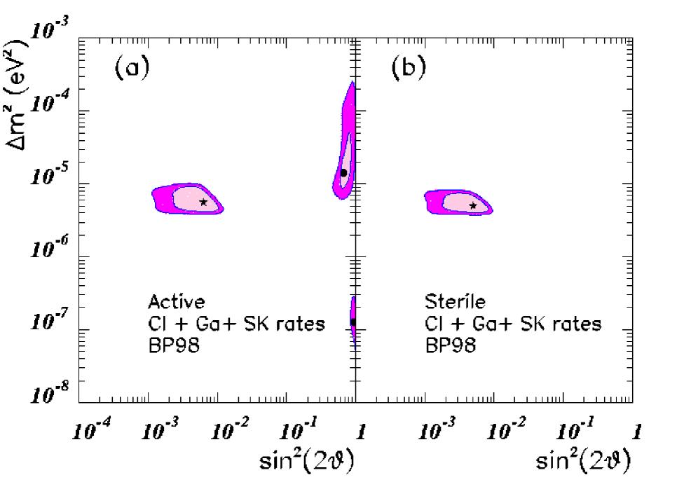
FIG. 2.: Allowed regions in $\Delta m^{2}$ and $\sin^{2}\theta$ from the measurements of the total event rates at Chlorine, Gallium and Super–Kamiokande (825-day data sample) for active-active transitions (a) and active-sterile (b). The darker (lighter) areas indicate the 99% (90%)CL regions. Global best–fit point is indicated by a star. Local best–fit points are indicated by a dot.

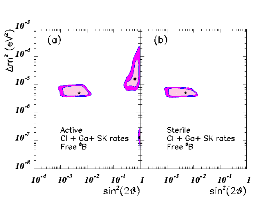
FIG. 3.: Same as previous figure but allowing a free ${}^{8}B$ flux normalization.

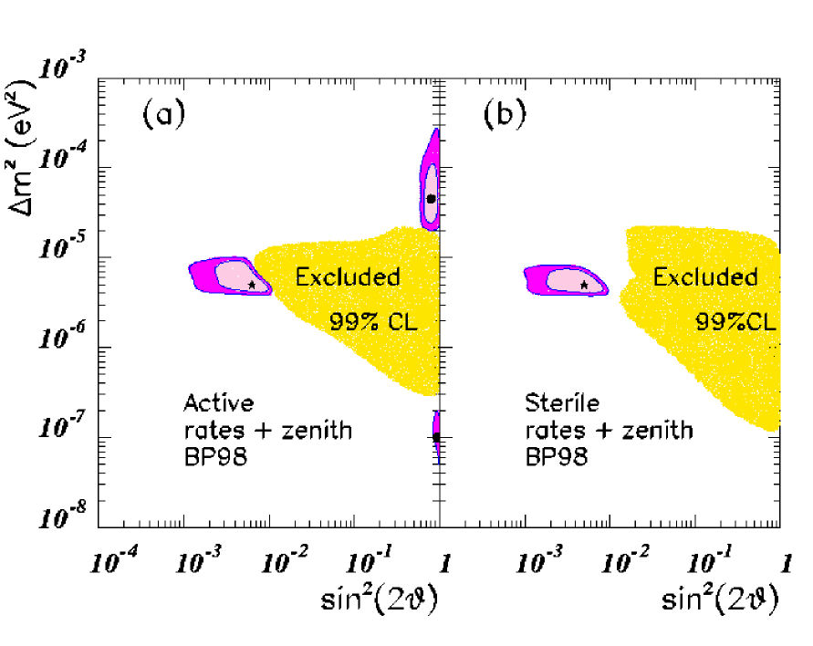
FIG. 4.: Allowed regions in $\Delta m^{2}$ and $\sin^{2}\theta$ from the measurements of the total event rates at Chlorine, Gallium and Super–Kamiokande (825-day data sample) combined with the zenith angle distribution observed in Super–Kamiokande for active-active (a) and active-sterile transitions (b). The darker (lighter) areas indicate 99% (90%)CL regions. Global best–fit point is indicated by a star. Local best–fit points are indicated by a dot. The shadowed area represents the region excluded by the zenith angle distribution data at 99% CL.

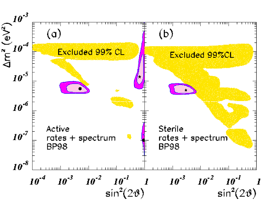
FIG. 5.: Allowed regions in $\Delta m^{2}$ and $\sin^{2}\theta$ from the measurements of the total event rates at the Chlorine, Gallium and Super–Kamiokande (825-day data sample) combined with the recoil electron spectrum data observed in Super–Kamiokande for active-active oscillations (a) and active-sterile oscillations (b) . The darker (lighter) area indicate 99% (90%)CL regions. Global best–fit point is indicated by a star. Local best–fit points are indicated by a dot. The shadowed area represents the region excluded by the spectrum data at (99%)CL.

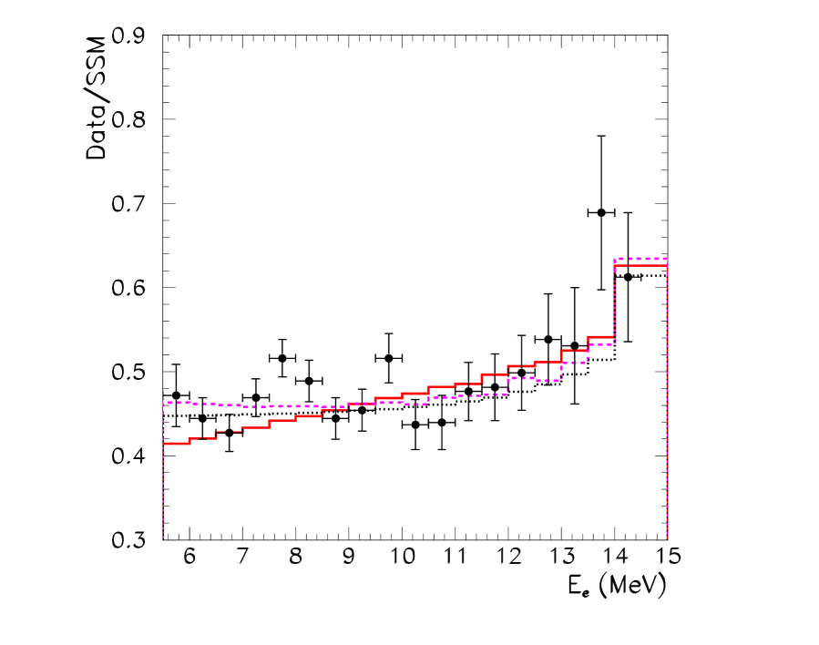
FIG. 6.: Expected normalized recoil electron energy spectrum compared with the experimental data [8]. The solid line represents the prediction for the best–fit SMA solution with free ${}^{8}B$ and $hep$ normalizations ($\beta=0.61$, $\gamma=12$), while the dashed line gives the corresponding prediction for the best–fit LMA solution ($\beta=1.37$, $\gamma=38$). Finally, the dotted line represents the prediction for the best non-oscillation scheme with free ${}^{8}B$ and $hep$ normalizations ($\beta=0.45$, $\gamma=13.5$).

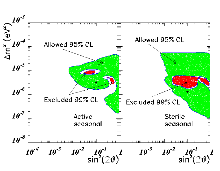
FIG. 7.: 95 and 99% CL regions obtained from the analysis of the seasonal dependence of the event rates observed in Super–Kamiokande from data with $E_{e}>11.5$ for active-active oscillations (a) and active-sterile oscillations (b). The larger area represents the allowed region at 95% CL. The darker area is the excluded region at 99% CL.

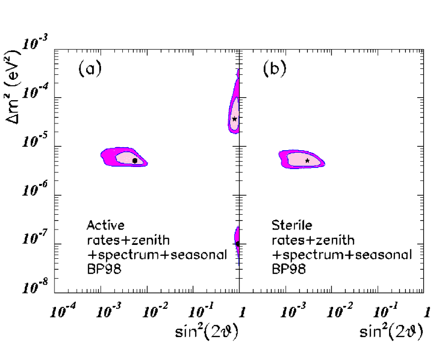
FIG. 8.: Allowed regions in $\Delta m^{2}$ and $\sin^{2}\theta$ from the measurements of the total event rates at the Chlorine, Gallium and Super–Kamiokande (825-day data sample) combined with the zenith angle distribution observed in Super–Kamiokande, the recoil energy spectrum and the seasonal dependence of the event rates, for active-active oscillations (a) and active-sterile oscillations (b) . The darker (lighter) areas indicate 99% (90%)CL regions. Global best–fit point is indicated by a star. Local best–fit points are indicated by a dot.

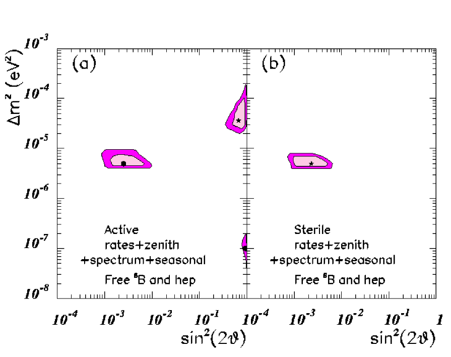
FIG. 9.: Same as previous figure allowing free ${}^{8}B$ and $hep$ neutrino flux normalizations.