Higgs Physics at a $\gamma\gamma$-Collider

Abstract

High precision measurements of electroweak observables at $e^{\pm}$ colliders indicate the existence of a light Higgs boson below the $W^{\pm}$ threshold. If such a fundamental scalar should be found in the near future it is important to fully investigate the electroweak symmetry braking sector of the Standard Model. This is particularly important for an intermediate mass Higgs as its existence might indicate physics beyond the Standard Model, for instance in form of its minimal supersymmetric extension (MSSM). In this work we present first results on the expected precision of the partial $\Gamma(H\longrightarrow\gamma\gamma)$ width at the $\gamma\gamma$ option of a future linear collider. This quantity is sensitive to new physics as heavy particles do not decouple in general and differences between the SM and MSSM predictions can differ by up to 10% even in the decoupling limit of large pseudoscalar Higgs masses. This regime is difficult and for some values of $\tan\beta$ impossible to cover at the LHC. We find that the well understood background process $\gamma\gamma\longrightarrow q\overline{q}$ allows for a ${\cal O}(2\%)$ determination of $\Gamma(H\longrightarrow\gamma\gamma)$ using conservative collider parameters.

1 Introduction

At a future linear $e^{\pm}$ collider the possibility of using Compton backscattered photons off the highly energetic and polarized incident electron beams [1, 2] can be used for many interesting physics applications. Important examples include the study of anomalous vector boson couplings through the large $W^{\pm}$ cross section, the search for heavy Higgs bosons up to $0.8\sqrt{s}$ (compared to $0.5\sqrt{s}$ in the $e^{\pm}$ mode), the CP-properties of fundamental scalars and the partial $\Gamma(H\longrightarrow\gamma\gamma)$ width (and thus the total Higgs-width assuming a knowledge of BR$(H\longrightarrow\gamma\gamma)$ from the LHC for instance). In addition one has the unique chance to study the polarized photon structure, complimentary processes involving supersymmetric particles (if they exist) at comparable event rates and, more exoticly, can even study theories predicting new dimensions at the TeV scale through Kaluzza-Klein excitations.

The main physics motivation of a future linear collider is not as much the discovery of new physics but its clarification. In analogous ways as SLC/LEP results have made precision tests of the SM after the discovery of massive vector bosons in hadronic collisions, the principle motivation for a linear collider is based on the hope that precise measurements of processes at the electroweak scale can shed light on the deeper structure of physical laws up to much higher energies, possibly GUT scales or evens regimes where the gravitational coupling becomes comparable to the other gauge couplings.

In this context the partial $\Gamma(H\longrightarrow\gamma\gamma)$ stands out as an observable of considerable theoretical and experimental importance. For intermediate mass Higgs bosons below 140 GeV it is the only decay channel accessible at the LHC as a relatively background free process [3]. At the Compton backscattered $\gamma\gamma$ option of the linear $e^{\pm}$ collider it represents the production process of a fundamental scalar. All charged particles contribute in the loop and heavy states which obtain their mass through the Higgs mechanism don’t decouple due to the Yukawa coupling at the vertex. Fig. 1 depicts the SM contributions from $W^{\pm}$ bosons and t-and b-quarks. In 2-Higgs Doublet Models (2HDM), such as in the Higgs sector of the MSSM, there are five fundamental scalars. The additional supersymmetry of the MSSM leads to only two free parameters of the electroweak braking sector, commonly chosen as the ratio of the vacuum expectation values of the up- and down-type Higgs bosons, $\tan\beta$, and the mass of the pseudoscalar Higgs boson, $m_{A}$. At tree level, all other masses and mixing angles are then fixed. The diphoton partial Higgs width prediction of the MSSM depends sensitively on these two parameters, even in the decoupling limit of large $m_{A}>500$ GeV. This regime, down to even lower $m_{A}$ for intermediate values of $\tan\beta$, is not covered at the LHC [3].

It is therefore important at this stage of the design of future collider schemes to investigate what the Compton collider option can contribute to the high precision measurements of the parameters of physics above the electroweak braking scales. In this context we summarize the status of the background (BG) process $\gamma\gamma\longrightarrow q\overline{q}$, $q=\{b,c\}$ relevant to the accurate determination of the signal (S) process $\gamma\gamma\longrightarrow H\longrightarrow b\overline{b}$ in the next section. We then discuss our jet definition and assumptions about the collider parameters and present first Monte Carlo results.

Figure 1: The Standard Model process $\gamma\gamma\longrightarrow H\longrightarrow b\overline{b}$ is mediated by $W-$boson and $t-$ and $b-$quark loops.

2 Radiative Corrections

The QCD corrections for both S and BG reactions are considerable and must be taken into account properly in order to precisely determine the diphoton Higgs width. In the next two sections we briefly summarize the radiative corrections relevant to our desired high ($\sim$ few %) accuracy for both processes.

2.1 The process $\gamma\gamma\longrightarrow q\overline{q}$

In this section we review the QCD corrections to the continuum heavy quark production in polarized photon-photon collisions. For the two possible $J_{z}$ states we have at the Born level:

$$\frac{d\sigma(\gamma\gamma(J_{z}=0)\longrightarrow q\overline{q})}{d\;\cos\;\theta} =$$

$$\frac{12\pi\alpha^{2}Q^{4}_{q}\beta}{s\;(1-\beta^{2}\cos^{2}\theta)^{2}}(1\!\!\!\!\! - \!\!\!\!\!\beta^{4})$$ (1)

$$\frac{d\sigma(\gamma\gamma(J_{z}=\pm 2)\longrightarrow q\overline{q})}{d\;\cos\;\theta} =$$

$$\frac{12\pi\alpha^{2}Q^{4}_{q}\beta^{3}}{s\;(1-\beta^{2}\cos^{2}\theta)^{2}}(1\!-\!\cos^{2}\theta)(2\!\!\!\!\!\! - \!\!\!\!\!\!\beta^{2}(1\!-\!\cos^{2}\theta))$$ (2)

where $\beta=\sqrt{1-4m^{2}_{q}/s}$ denotes the quark velocity, $\sqrt{s}\equiv w$ the $\gamma\gamma$ c.m. collision energy, $\alpha^{-1}\approx 128$ the electromagnetic coupling, $Q_{q}$ the charge of quark $q$ and $m_{q}$ its pole mass. The scattering angle of the produced (anti)quark relative to the beam direction is denoted by $\theta$. Eq. 1 clearly displays the important feature that the $J_{z}=0$ cross section has a relative $\frac{m^{2}_{q}}{s}$ suppression compared to the $J_{z}=\pm 2$ cross section. Since the Higgs $\gamma\gamma\to H\to q\overline{q}$ process only occurs for $J_{z}=0$, it is this polarization that is crucial for the precision measurement of the Higgs partial decay width.

There are, however, important radiative corrections to the $J_{z}=0$ cross section as large non-Sudakov double logarithm enter into loop effects [4] and real Bremsstrahlung corrections can even remove the mass suppression [5]. In this work we will include the exact one loop corrections of Ref. [4] (for both spin configurations) and use the recently achieved all orders resummed DL-result of Ref. [6] for $J_{z}=0$:

$$\sigma^{DL}_{{\rm virt}+{\rm soft}}\!\!\! = \!\!\!\sigma_{\rm Born}\left\{1+{\cal F}\;\;_{2}F_{2}(1,1;2,\frac{3}{2};\frac{1}{2}{\cal F})\right.$$ (3)

$$\!\!\!\left.+2\;{\cal F}\;\;_{2}F_{2}(1,1;2,\frac{3}{2};\frac{C_{A}}{4C_{F}}{\cal F})\right\}^{2}\times$$

$$\!\!\!\exp\left(\frac{\alpha_{s}C_{F}}{\pi}\left[\log\frac{s}{m_{q}^{2}}\left(\frac{1}{2}-\log\frac{s}{4l_{c}^{2}}\right)\right.\right.$$

$$\!\!\!\left.\left.+\log\frac{s}{4l_{c}^{2}}-1+\frac{\pi^{2}}{3}\right]\right)$$

where ${\cal F}=-C_{F}\frac{\alpha_{s}}{4\pi}\log^{2}\frac{s}{m_{q}^{2}}$ is the one-loop hard form factor, $\alpha_{s}$ is taken as a fixed parameter, and $l_{c}\ll\sqrt{s}$ is the soft-gluon upper energy limit.

In Ref. [7] it was pointed out that one needs to include at least four loops (at the cross section level) of the non-Sudakov hard logarithms in order to achieve positivity and stability. At this level of approximation there is an additional major source of uncertainty in the scale choice of the QCD coupling, two possible ‘natural’ choices — $\alpha_{s}(m_{H}^{2})$ and $\alpha_{s}(m_{q}^{2})$ — yielding very different numerical results. These uncertainties were removed in Ref. [8] by employing a running coupling into each loop integration. The correct running scale was found to be ${\bf l_{\perp}^{2}}$ in terms of the perpendicular Sudakov components and was implemented by using

$$\alpha_{s}({\bf l^{2}_{\perp}})\!\!\!\! = \!\!\!\!\frac{\alpha_{s}(m^{2})}{1\!+\!\left(\beta_{0}\frac{\alpha_{s}(m^{2})}{\pi}+\beta_{1}\left(\frac{\alpha_{s}(m^{2})}{\pi}\right)^{2}\right)\log\frac{{\bf l^{2}_{\perp}}}{m^{2}}}$$ (4)

$$\equiv \!\!\!\!\frac{\alpha_{s}(m^{2})}{1+c\;\log\frac{{\bf l^{2}_{\perp}}}{m^{2}}}$$

where $\beta_{0}=\frac{11}{12}C_{A}-\frac{4}{12}T_{F}n_{F}$, $\beta_{1}=\frac{17}{24}C_{A}^{2}-\frac{5}{12}C_{A}T_{F}n_{F}-\frac{1}{4}C_{F}T_{F}n_{F}$ and for QCD we have $C_{A}=3$, $C_{F}=\frac{4}{3}$ and $T_{F}=\frac{1}{2}$ as usual. Up to two loops the massless $\beta$-function is independent of the chosen renormalization scheme and is gauge invariant in minimally subtracted schemes to all orders. These features also hold for the renormalization group (RG) improved form factors below and lead to [8]:

$$\frac{\sigma^{DL}_{RG}}{\sigma_{\rm Born}}=\left\{1+\widetilde{{\cal F}}_{h}^{RG}\right\}^{2}\exp\left(\widetilde{{\cal F}}^{RG}_{S_{R}}+2\widetilde{{\cal F}}^{RG}_{S_{V}}\right)$$ (5)

where the RG-massive Sudakov form factor is given by:

$$\widetilde{{\cal F}}^{RG}_{S_{R}}+2\widetilde{{\cal F}}^{RG}_{S_{V}}\!\!\!\! = \!\!\!\!\frac{\alpha_{s}(m^{2})C_{F}}{\pi}\left\{\frac{1}{c}\int_{\frac{2l_{c}m^{2}}{(s+m^{2})\sqrt{s}}}^{\frac{2l_{c}\sqrt{s}}{s+m^{2}}}\frac{d\beta_{1}}{\beta_{1}}\times\right.$$ (6)

$$\!\!\!\!\log\frac{1+c\;\log\left(\left(\frac{2l_{c}}{\sqrt{s}}-\beta_{1}\right)\beta_{1}\frac{s}{m^{2}}\right)}{\left(1+c\;\log\frac{s\beta_{1}}{m^{2}}\right)}$$

$$\!\!\!\!-\frac{1}{c}\log\frac{s}{m^{2}}\log\frac{\alpha_{s}(2l_{c}\sqrt{s})}{\alpha_{s}(s)}$$

$$\!\!\!\!-\frac{1}{c}\log\frac{2l_{c}}{\sqrt{s}}\log\frac{\alpha_{s}(2l_{c}\sqrt{s})}{\alpha_{s}\left(\frac{2l_{c}m^{2}}{\sqrt{s}}\right)}$$

$$\!\!\!\!-\frac{1}{c^{2}}\log\frac{\alpha_{s}(m^{2})\alpha_{s}(2l_{c}\sqrt{s})}{\alpha_{s}(s)\alpha_{s}\left(\frac{2l_{c}m^{2}}{\sqrt{s}}\right)}$$

$$\!\!\!\!\left.+\!\frac{1}{2}\log\frac{s}{m^{2}}\!+\!\log\frac{s}{4l_{c}^{2}}\!-\!1\!+\!\frac{\pi^{2}}{3}\!\right\}$$

Figure 2: The effect of the renormalization group improved form factor (circles) of Eq. 5 in comparison to using the DL form factors of Eq. 3 with the indicated values of the strong coupling. The energy cutoff is chosen to be $l_{c}=0.1\sqrt{s}$. The effect is displayed for the bottom quark with $m_{b}=4.5$ GeV.

and the hard (non-Sudakov) RG form factor by:

$$\widetilde{{\cal F}}_{h}^{RG} = \sum^{\infty}_{i=0}\int^{s}_{m^{2}}\frac{d{\bf l^{2}_{\perp}}}{{\bf l^{2}_{\perp}}}\left(\frac{C_{F}}{2\pi}\right)^{i+1}\left(\frac{\alpha_{s}(m^{2})}{c}\right)^{i}\times$$ (7)

$$\frac{\alpha_{s}({\bf l^{2}_{\perp}})}{(i+1)!}\log^{i+1}\frac{{\bf l^{2}_{\perp}}}{s}\log^{i}\frac{\alpha_{s}(m^{2})}{\alpha_{s}({\bf l^{2}_{\perp}})}+$$

$$2\sum^{\infty}_{i=0}\int^{s}_{m^{2}}\frac{d{\bf l^{2}_{\perp}}}{{\bf l^{2}_{\perp}}}\frac{C_{F}C_{A}^{i}}{2^{2i+1}\pi^{i+1}}\left(\frac{\alpha_{s}(m^{2})}{c}\right)^{i}\times$$

$$\frac{\alpha_{s}({\bf l^{2}_{\perp}})}{(i+1)!}\log^{i+1}\frac{{\bf l^{2}_{\perp}}}{s}\log^{i}\frac{\alpha_{s}(m^{2})}{\alpha_{s}({\bf l^{2}_{\perp}})}$$

The effect of using the RG-form factors compared to the DL resummed result is displayed in Fig. 2. Here we choose the gluon energy cut $l_{c}=0.1\sqrt{s}$. At one loop there is no $l_{c}$ dependence while at higher orders there inevitably is.

2.2 The process $\gamma\gamma\longrightarrow H\longrightarrow b\overline{b}$

An intermediate mass Higgs boson has a very narrow total decay width. It is therefore appropriate to compare the total number of Higgs signal events with the number of (continuum) background events integrated over a narrow energy window around the Higgs mass. The size of this window depends on the level of monochromaticity that can be achieved for the polarized photon beams.

In general, the number of events for the (signal) process $S$ is given by

$$N_{S}=\int\frac{dL}{dw}\sigma_{S}(w)dw$$ (8)

where $w$ denotes the center of mass energy. For $S\equiv\gamma\gamma\longrightarrow H\longrightarrow b\overline{b}$ we have the following Breit-Wigner cross section [5]

$$\sigma_{S}(w)=\frac{16\pi\Gamma(H\longrightarrow\gamma\gamma)\Gamma(H\longrightarrow b\overline{b})}{(w^{2}-m^{2}_{H})^{2}+\Gamma_{H}^{2}m^{2}_{H}}(\hbar c)^{2}$$ (9)

where the conversion factor $(\hbar c)^{2}=3.8937966\times 10^{11}$ fb GeV². In the narrow width approximation we then find for the expected number of events

$$\frac{N_{S}}{(\bar{h}c)^{2}}\!\!=\!\!\left.\frac{dL_{\gamma\gamma}}{dw}\right|_{m_{H}}\!\!\!\!\!\!\!\!\frac{8\pi^{2}\Gamma(H\!\!\longrightarrow\gamma\gamma)BR(H\!\!\longrightarrow b\overline{b})}{m^{2}_{H}}$$ (10)

To quantify this, we take the design parameters of the proposed TESLA linear collider [9], which correspond to an integrated peak $\gamma\gamma$-luminosity of 15 fb^-1 for the low energy running of the Compton collider. The polarizations of the incident electron beams and the laser photons are chosen such that the product of the helicities $\lambda_{e}\lambda_{\gamma}=-1$. This ensures high monochromaticity and polarization of the photon beams. In this scenario we find a typical Higgs mass resolution of 10 GeV, so that for the background process $BG\equiv\gamma\gamma\longrightarrow q\overline{q}$ we use

$$\frac{L_{\gamma\gamma}}{10\;{\rm GeV}}=\left.\frac{dL_{\gamma\gamma}}{dw}\right|_{m_{H}}$$ (11)

with $\left.\frac{dL_{\gamma\gamma}}{dw}\right|_{m_{H}}=$0.5 fb^-1/GeV. The number of background events is then given by

$$N_{BG}=L_{\gamma\gamma}\sigma_{BG}$$ (12)

In other words, the number of signal events is proportional to $N_{S}\sim\left.\frac{dL_{\gamma\gamma}}{dw}\right|_{m_{H}}$ while the number of continuum heavy quark production events is proportional to $N_{BG}\sim L_{\gamma\gamma}$. In principle it is possible to use the exact Compton profile of the backscattered photons to obtain the full luminosity distributions. The number of expected events is then given as a convolution of the energy dependent luminosity and the cross sections. Our approach described above corresponds to an effective description of these convolutions, since these functions are not precisely known at present. Note that the functional forms currently used generally assume that only one scattering takes place for each photon, which may not be realistic. Once the exact luminosity functions are experimentally determined it is of course trivial to incorporate them into a Monte Carlo program containing the physics described in this paper.

We next summarize the radiative corrections entering into the calculation of the expected number of Higgs events. For the quantity $\Gamma(H\longrightarrow\gamma\gamma)$ there are three main Standard Model contributions, depicted in Fig. 1: the $W^{\pm}$ and $t-$ and $b-$quark loops. We include these at the one loop level, since the radiative corrections are significant only for the $b-$quark. The branching ratio $BR(H\longrightarrow b\overline{b})$ is treated in the following way. The first component consists of the partial $\Gamma(H\longrightarrow b\overline{b})$ width. Obviously we must use the same two-jet criterion for the signal as for the background. For our purposes a cone-type algorithm is most suitable, and so we use the Sterman-Weinberg two-jet definition depicted in Fig. 3. Note that the signal cross section is corrected by the same resummed renormalization group improved form factor given in Eq. 6, since this factor does not depend on the spin of the particle coupling to the final state quark anti-quark pair.

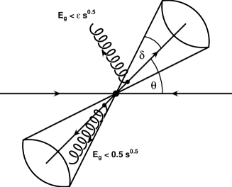
Figure 3: The parameters of the Sterman-Weinberg two jet definition used in this work. Inside an angular cone of size $\delta$ arbitrary hard gluon Bremsstrahlung is included. Radiation outside this cone is only permitted if the gluon energy is below a certain fraction ($\epsilon$) of the incident center of mass energy. The thrust angle is denoted by $\theta$.

Figure 4: The number of both signal and background events for jet parameters $\epsilon=0.1$ and $\delta=20^{o}$ and the indicated values of the thrust angle $\theta$. The upper row assumes a ratio of $J_{0}/J_{2}=20$ and the lower row of $50$. The background is composed of bottom and charm contributions assuming 70 % double b-tagging efficiency and a 3 % probability to count a $c\overline{c}$ pair as $b\overline{b}$. The dash-dot line corresponds to $J_{z}=\pm 2$ for $m_{c}$, the full line to $J_{z}=0$ for $m_{b}$, the dotted line to $J_{z}=\pm 2$ for $m_{b}$ and the dashed line to $J_{z}=0$ for $m_{c}$. All lines are are normalized to add up to the total background and all radiative corrections discussed in the text are included.

In addition we use the exact one-loop corrections from Ref. [10]. These revealed that the largest radiative corrections are well described by using the running quark mass evaluated at the Higgs mass scale. We therefore resum the leading running mass term to all orders. For the real Bremsstrahlung corrections we use our own $H\longrightarrow q\bar{q}g$ matrix elements. An important check is obtained by integrating over all phase space and reproducing the analytical results of Ref. [10].

The second quantity entering the branching ratio is the total Higgs width $\Gamma_{H}$. Here we use the known results summarized in Ref. [3], and include the partial Higgs to $b\overline{b}$, $c\overline{c}$, $\tau^{\pm}$, $WW^{*}$, $ZZ^{*}$ and $gg$ decay widths with all relevant radiative corrections.

3 Numerical Results

Figure 5: The ratio of signal to background events based on the jet parameters of Fig. 4. The smaller phase space cut $|\cos\theta|<0.5$ gives a larger ratio as expected.

Figure 6: The statistical accuracy of the measurement based on a one year running with the parameters of Fig. 4. Surprisingly the larger thrust angle cuts gives a slightly better statistical significance.

In this section we are presenting first (conservative) results based on the minimally achievable detector performance expected for the Tesla design [11]. All relevant radiative corrections discussed above are included and the two jet definition is the one discussed in Ref. [8] based on Sterman-Weinberg parameters and identifying $\epsilon\sqrt{s}\equiv l_{c}$. We thus arrive at

$$\sigma_{\rm 2j}=\sigma^{DL}_{RG}(\epsilon\sqrt{s})+\tilde{\sigma}_{\rm SV}+\sigma_{\rm H}(\epsilon\sqrt{s},\epsilon,\delta)\;.$$ (13)

where the three contributions contain the RG-improved form factors, the exact one loop subleading corrections and the hard Bremsstrahlung radiation inside the cone of half-angle $\delta=20^{o}$ respectively. Fig. 4 assumes a 70% double b-tagging efficiency and a 3% probability of counting a $c\overline{c}$-pair as a $b\overline{b}$-pair. The figures show two curves for a ratio of $J_{0}/J_{2}=20$ and $50$ as well as differing cuts on the jet thrust angle $\theta$. One can see clearly that a high charm suppression rate is highly desirable. While the larger thrust angle cut $|\cos\theta|<0.5$ leads to a larger ratio of S to BG events (see Fig. 5), the inverse statistical significance, displayed in Fig. 6, is slightly lower for $|\cos\theta|<0.7$. Although several questions concerning the dependence of these Monte Carlo results on the various jet parameters should be addressed more carefully, it seems safe to assume that statistically an ${\cal O}(2\%)$ measurement for the diphoton partial Higgs width is feasible. More thorough investigations will be presented in Ref. [12].

4 Conclusions

In this paper we have included all available and relevant radiative corrections for the measurement of the partial Higgs width $\Gamma(H\longrightarrow\gamma\gamma)$. Conservative assumptions about the expected machine and detector parameters lead to the preliminary result that over a four years of running time the diphoton partial width can be measured with a statistical uncertainty of ${\cal O}(2\%)$. This level of precision could be very important for large pseudoscalar Higgs masses in theories, such as the MSSM, with extended Higgs sectors and could significantly enhance the kinematical reach for new physics.

References

- [1] I.F. Ginzburg et al., Nucl.Inst.Meth. 205 (1983) 47 & Nucl.Inst.Meth. 219 (1984) 5.
- [2] V.I. Telnov, Nucl.Inst.Meth. A 355 (1995) 5.
- [3] M. Spira, hep-ph/9705337, Fortsch.Phys. 46:203-284,1998.
- [4] G. Jikia, A. Tkabladze, Phys. Rev. D 54 (1996) 2030 and Nucl. Inst. Meth. A 355 (1995) 81.
- [5] D.L. Borden, V.A. Khoze, J. Ohnemus and W.J. Stirling, Phys. Rev. D 50 (1994) 4499.
- [6] M. Melles, W.J. Stirling, hep-ph/9807332, to appear in Phys. Rev. D.
- [7] M. Melles, W.J. Stirling, hep-ph/9810432, to appear in Eur. Phys. J.
- [8] M. Melles, W.J. Stirling, hep-ph/9903507, to appear in Nucl. Phys. B.
- [9] V.I. Telnov, private communications.
- [10] E. Braaten, J.P. Leveille, Phys.Rev.D22 (1980) 715.
- [11] M. Battaglia, private communications.
- [12] M. Melles, W.J. Stirling, V.A. Khoze, to be published.