Theory of $Z$ boson decays

Abstract

The precision data on $Z$ boson decays from LEP-I and SLC colliders are compared with the predictions based on the Minimal Standard Theory. The Born approximation of the theory is based on three most accurately known observables: $G_{\mu}$ – the four fermion coupling constant of muon decay, $m_{Z}$ – the mass of the $Z$ boson, and $\alpha(m_{Z})$ – the value of the “running fine structure constant” at the scale of $m_{Z}$. The electroweak loop corrections are expressed, in addition, in terms of the masses of higgs, $m_{H}$, of the top and bottom quarks, $m_{t}$ and $m_{b}$, and of the strong interaction constant $\alpha_{s}(m_{Z})$. The main emphasis of the review is focused on the one-electroweak-loop approximation. Two electroweak loops have been calculated in the literature only partly. Possible manifestations of new physics are briefly discussed.

Contents.

1. Introduction.

2. Basic parameters of the theory.

3. Amplitudes, widths, and asymmetries.

4. One-loop corrections to hadronless observables.
                     4.1 Four types of Feynman diagrams.
                     4.2 The asymptotic limit at $m_{t}^{2}\gg m_{Z}^{2}$.
                     4.3 The functions $V_{m}(t,h)$, $V_{A}(t,h)$ and $V_{R}(t,h)$.
                     4.4 Corrections $\delta V_{i}(t)$.
                     4.5 Accidental (?) compensation and the mass of the $t$-quark.
                     4.6 How to calculate $V_{i}$? ‘Five steps’.

5. One-loop corrections to hadronic decays of the $Z$ boson.
                     5.1 The leading quarks and hadrons.
                     5.2 Decays to pairs of light quarks.
                     5.3 Decays to $b\bar{b}$ pair.

6. Comparison of one-electroweak-loop results and experimental LEP-I and SLC data.
                     6.1 LEPTOP code.
                     6.2 One-loop general fit.

7. Two-loop electroweak corrections and theoretical uncertainties.
                     7.1 $\alpha_{W}^{2}t^{2}$ corrections to $m_{W}/m_{Z}$ , $g_{A}$ and $g_{V}/g_{A}$ from reducible diagrams.
                     7.2 $\alpha^{2}_{W}t^{2}$ corrections from irreducible diagrams.
                     7.3 $\alpha^{2}_{W}t$ corrections and the two-loop fit of experimental data.
   

8. Extensions of the Standard Model.
                     8.1 Sequential heavy generations in the Standard Model.
                     8.2 SUSY extensions of the Standard Model.
   

9. Conclusions.

Appendix A. Regularization of Feynman integrals.

Appendix B. Relation between $\bar{\alpha}$ and $\alpha(0)$.

Appendix C. How $\alpha_{W}(q^{2})$ and $\alpha_{Z}(q^{2})$ ‘crawl’.

Appendix D. General expressions for one-loop corrections to hadronless observables.

Appendix E. Radiators $R_{Aq}$ and $R_{Vq}$.

Appendix F. $\alpha_{W}^{2}t^{2}$ corrections from reducible diagrams.

Appendix G. Oblique corrections from new generations and SUSY.

Appendix H. Other parametrizations of radiative corrections.

References.

Figure captions.

1 Introduction

$Z$ boson, electrically neutral vector boson (its spin equals 1) with mass $m_{Z}\simeq 91$ GeV and width $\Gamma_{Z}\simeq 2.5$ GeV, occupies a unique place in physics. This heavy analog of the photon was experimentally discovered in 1983, practically simultaneously with its charged counterparts $W^{\pm}$ bosons with mass $m_{W}\simeq 80$ GeV and width $\Gamma_{W}\simeq 2$ GeV [1].

The discovery was crowned by Nobel Prize to Carlo Rubbia (for the bosons) and to Simon van der Meer (for the CERN proton-antiproton collider, which was specially constructed to produce $W$ and $Z$ bosons) [2].

The extremely short-lived vector bosons ($\tau=1/\Gamma\simeq 10^{-25}$ sec) were detected by their decays into various leptons and hadrons. The detectors, in which these decay products were observed, were built and operated by collaborations of physicists and engineers the largest in the previous history of physics.

The discovery of $W$ and $Z$ bosons was a great triumph of experimental physics, but even more so of theoretical physics. The masses and widths of the particles, the cross-sections of their production turned out to be in perfect agreement with the predictions of electroweak theory of Sheldon Glashow, Abdus Salam and Steven Weinberg [3]. The theory was so beautiful that its authors received the Nobel Prize already in 1979 [4], four years before its crucial confirmation.

The electroweak theory unified two types of fundamental interactions: electromagnetic and weak. The theory of electromagnetic interaction – quantum electrodynamics, or QED, was cast in its present relativistically covariant form in the late 1940’s and early 1950’s and served as a “role model” for the relativistic field theories of two other fundamental interactions: weak and strong.

The main virtue of QED was its renormalizability. Let us explain this “technical” term by using the example of interaction of photons with electrons. One can find systematic presentation in modern textbooks [5]. In the lowest approximation of perturbation theory (the so called tree approximation in the language of Feynman diagrams) all electromagnetic phenomena can be described in terms of electric charge and mass of the electron ($e$, $m$). The small parameter of perturbation theory is the famous $\alpha=e^{2}/4\pi\simeq 1/137$.

The problem with any quantum field theory is that in higher orders of perturbation theory, described by Feynman graphs with loops, the integrals over momenta of virtual particles have ultraviolet divergences, so that all physical quantities including electric charge and mass of the electron themselves become infinitely large. To avoid infinities an ultraviolet cut-off $\Lambda$ could be introduced. Another, more sophisticated method is to use dimensional regularization: to calculate the Feynman integrals in momentum space of $D$ dimensions. These integrals diverge at $D=4$, but are finite, proportional to $1/\varepsilon$ in vicinity of $D=4$, where by definition $2\varepsilon=4-D\to 0$ (see Appendix A).

The theory is called renormalizable, if one can get rid of this cut-off (or $1/\varepsilon$) by establishing relations between observables only. In the case of electrons and photons such basic observables are physical (renormalized) charge and mass of the electron. This allows to calculate higher order effects in $\alpha$ and compare the theoretical predictions with the results of high precision measurements of such observables as e.g. anomalous magnetic moments of electron or muon.

The renormalizability of electrodynamics is guaranteed by the dimensionless nature of the coupling constant $\alpha$ and by conservation of electric current.

After this short description of QED let us turn to the weak interaction.

The first manifestation of the weak interaction was discovered by Henri Becquerel at the end of the XIX century. Later this type of radioactivity was called $\beta$-decay. The first theory of $\beta$-decay was proposed by Enrico Fermi in 1934 [6]. The theory was modelled after quantum electrodynamics with two major differences: first, instead of charge conserving, “neutral”, electrical current of the type $-\bar{e}\gamma_{\alpha}e+\bar{p}\gamma_{\alpha}p$ there were introduced two charge changing, “charged”, vector currents: one for nucleons, transforming neutron into a proton, $\bar{p}\gamma_{\alpha}n$, another for leptons, transforming neutrino into electron or creating a pair: electron plus antineutrino, $\bar{e}\gamma_{\alpha}\nu$. (Here $\bar{e}(e)$ denotes operator, which creates (annihilates) electron and annihilates (creates) positron. The symbols of other particles have similar meaning; $\gamma_{\alpha}$ are four Dirac matrices, $\alpha=0,1,2,3$.)

The second difference between the Fermi theory and electrodynamics was that the charged currents interacted locally via four fermion interaction:

$$G\cdot\bar{p}\gamma_{\alpha}n\cdot\bar{e}\gamma_{\alpha}\nu+\mbox{\rm h.c.}\;\;,$$ (1)

where summation over index $\alpha$ is implied (in this summation we use Feynman’s convention: $+$ for $\alpha=0$ and $-$ for $\alpha=1,2,3$); h.c. means hermitian conjugate. The coupling constant $G$ of this interaction was called Fermi coupling constant.

From simple dimensional considerations it is evident that dimension of $G$ is (mass)^-2 and therefore the four-fermion interaction is not renormalizable, the higher orders being divergent as $G^{2}\Lambda^{2}$, $G^{3}\Lambda^{4}$ … . Why these divergent corrections still allow one to rely on the lowest order approximation, remained a mystery. But for many years the lowest order four-fermion interaction served as a successful phenomenological theory of weak interactions.

It is in the framework of this phenomenological theory that a number of subsequent experimental discoveries were accommodated. First, it turned out that $\beta$-decay is one of the large family of weak processes, involving newly discovered particles, such as pions, muons and muonic neutrinos, strange particles, etc. Second, it was discovered that all these processes are caused by selfinteraction of one weak charged current, involving leptonic and hadronic terms. Later on, when the quark structure of hadrons was established, the hadronic part of the current was expressed through corresponding quark current. Third, it was established in 1957 that all weak interactions violate parity conservation $P$ and charge conjugation invariance $C$. This violation turned out to have a universal pattern: the vector form of the current $V$, introduced by Fermi, was substituted [7] by one half of the sum of vector and axial vector, $A$, which meant that $\gamma_{\alpha}$ should be substituted by $\frac{1}{2}\gamma_{\alpha}(1+\gamma_{5})$.

In other words one can say that fermion $\psi$ enters the charged current only through its left-handed chiral component

$$\psi_{L}=\frac{1}{2}(1+\gamma_{5})\psi$$ (2)

From such structure of the charged current it follows that the corresponding antifermions interact only through their right-handed components.

Attempts to construct a renormalizable theory of weak interaction resulted in a unified theory of electromagnetic and weak interactions – the electroweak theory [3, 4] with two major predictions. The first prediction was the existence alongside with the charged weak current also of a neutral weak current. The second prediction was the existence of the vector bosons: $Z$ coupled to the weak neutral current and $W^{+}$ and $W^{-}$ coupled to the charged current (like $\frac{1}{2}\bar{e}\gamma_{\alpha}(1+\gamma_{5})\nu$) and its hermitian conjugate current (like $\frac{1}{2}\bar{\nu}\gamma_{\alpha}(1+\gamma_{5})e$).

The vector bosons were massive analogues of the photon $\gamma$; their couplings to the corresponding currents, $f$ and $g$, were the analogues of the electric charge $e$. Thus $\alpha_{Z}=f^{2}/4\pi$ and $\alpha_{W}=g^{2}/4\pi$ were dimensionless like $\alpha=e^{2}/4\pi$, which was a necessary (but not sufficient) condition of renormalizability of the weak interaction.

The first theory, involving charged vector bosons and photon, was proposed by Oscar Klein just before World War II [8]. Klein based his theory on the notion of local isotopic symmetry: he considered isotopic doublets $(p,n)$ and $(\nu,e)$, and isotopic triplet $(B^{+},A^{0},B^{-})$. Where $B^{\pm}$ denoted what we call now $W^{\pm}$, while $A^{0}$ was electromagnetic field. He also mentioned the possibility to incorporate a neutral massive field $C^{0}$ (the analogue of our $Z^{0}$). In fact this was the first attempt to construct a theory based on a non-abelian gauge symmetry, with vector fields playing the role of gauge fields. The gauge symmetry was essential for conservation of the currents. Unfortunately, Klein did not discriminate between weak and strong interaction and his paper was firmly forgotten.

The non-abelian gauge theory was rediscovered in 1954 by C.N.Yang and R.Mills [9] and became the basis of the so-called Standard Model with its colour $SU(3)_{c}$ group for strong interaction of quarks and gluons and $SU(2)_{L}\times U(1)_{Y}$ group for electroweak interaction (here indices denote: $c$ – colour, $L$ – weak isospin of left-handed spinors, and $Y$ – the weak hypercharge). The electric charge $Q=T_{3}+Y/2$, where $T_{3}$ is the third projection of isospin. $Y=1/3$ for a doublet of quarks, $Y=-1$ for a doublet of leptons. As for the right-handed spinors, they are isosinglets, and hence

$$Y(\nu_{R})=0\;,\;\;Y(e_{R})=-2\;,\;\;Y(u_{R})=4/3\;,\;\;Y(d_{R})=-2/3\;\;.$$

Thus, parity violation and charge conjugation violation were incorporated into the foundation of electroweak theory.

Out of the four fields (three of $SU(2)$ and one of $U(1)$, usually denoted by $W^{+},W^{0},W^{-}$ and $B^{0}$, respectively) only two directly correspond to the observed vector bosons: $W^{+}$ and $W^{-}$. The $Z^{0}$ boson and photon are represented by two orthogonal superpositions of $W^{0}$ and $B^{0}$:

$$Z^{0} = cW^{0}-sB^{0}$$ (3)

$$A^{0} = sW^{0}+cB^{0}\;\;,$$

where $c=\cos\theta$, $s=\sin\theta$, while the weak angle $\theta$ is a free parameter of electroweak theory. The value of $\theta$ is determined from experimental data on $Z$ boson coupling to neutral current. The “$Z$-charge”, characterizing the coupling of $Z$ boson to a spinor with definite helicity is given by

$$\bar{f}(T_{3}-Qs^{2})\;\;,$$ (4)

where

$$\bar{f}=\bar{g}/c\;\;.$$ (5)

Note that the “$Z$-charge” is different for the right- and left-handed spinors with the same value of $Q$ because they have different values of $T_{3}$. The coupling constant of $W$-bosons is also expressed in terms of $\bar{e}$ and $\theta$:

$$\bar{g}=\bar{e}/s\;\;.$$ (6)

The theory described above has many nice features, the most important of which is its renormalizability. But at first sight it looks absolutely useless: all fermions and bosons in it are massless. This drawback cannot be fixed by simply adding mass terms to the Lagrangian. The mass terms of fermions would contain both $\psi_{L}$ and $\psi_{R}$ and thus explicitly break the isotopic invariance and hence renormalizability. The gauge invariance would also be broken by the mass terms of the vector bosons. All this would result in divergences of the type $\Lambda^{2}/m^{2}$, $\Lambda^{4}/m^{4}$, etc.

The way out of this trap is the so called Higgs mechanism [10]. In the framework of the Minimal Standard Model the problem of mass is solved by postulating the existence of the doublet $\varphi_{H}=(\varphi^{+},\varphi^{0})$ and corresponding antidoublet $(\bar{\varphi}^{0},-\varphi^{-})$ of spinless particles. These four bosons differ from all other particles by the form of their self-interaction, the energy of which is minimal when the neutral field $\varphi_{1}=\frac{1}{\sqrt{2}}(\varphi^{0}+\bar{\varphi}^{0})$ has a nonvanishing vacuum expectation value. The isospin of the Higgs doublet is $1/2$, its hypercharge is $1$. Thus, it interacts with all four gauge bosons. In particular, it has quartic terms $\frac{1}{4}\bar{g}^{2}\bar{W}W\varphi_{1}^{2}$,     $\frac{1}{8}\bar{f}^{2}\bar{Z}Z\varphi_{1}^{2}$, which give masses to the vector bosons when $\varphi_{1}$ acquires its vacuum expectation value (vev) $\eta$:

$$m_{W}=\bar{g}\eta/2\;,\;\;m_{Z}=\bar{f}\eta/2\;\;.$$ (7)

The magnitude of $\eta$ can easily be derived from that of the four-fermion interaction constant $G_{\mu}$ in muon decay:

$$\frac{G_{\mu}}{\sqrt{2}}\cdot\bar{\nu}_{\mu}\gamma_{\alpha}(1+\gamma_{5})\mu\cdot\bar{e}\gamma_{\alpha}(1+\gamma_{5})\nu_{e}\;\;.$$ (8)

In the Born approximation of electroweak theory this four-fermion interaction is caused by an exchange of a virtual $W$-boson (see Figure 1). Hence

$$\frac{G_{\mu}}{\sqrt{2}}=\frac{g^{2}}{8m_{W}^{2}}=\frac{\bar{g}^{2}}{8m_{W}^{2}}\;,\;\;\eta=(\sqrt{2}G_{\mu})^{-1/2}=246\;\mbox{\rm GeV}\;\;.$$ (9)

Such mechanism of appearance of masses of $W$ and $Z$ bosons is called spontaneous symmetry breaking. It preserves renormalizability [11]. (As a hint, one can use the symmetrical form of Lagrangian by not specifying the vev $\eta$.)

The fermion masses can be introduced also without explicitly breaking the gauge symmetry. In this case the mass arises from an isotopically invariant term $f_{Y}\cdot\varphi_{H}\bar{\psi}_{L}\psi_{R}+{\rm h.c.}$, where $f_{Y}$ is called Yukawa coupling. The mass of a fermion $m=f_{Y}\eta/\sqrt{2}$. There is a separate Yukawa coupling for each of the known fermions. Their largely varying values are at present free parameters of the theory and await for the understanding of this hierarchy.

Let us return for a moment to the vector bosons. A massless vector boson (e.g. photon) has two spin degrees of freedom – two helicity states. A massive vector boson has three spin degrees of freedom corresponding, say, projections $\pm 1,0$ on its momentum. Under spontaneous symmetry breaking three out of four spinless states, $\varphi^{\pm},\varphi_{2}^{0}=\frac{1}{\sqrt{2}}(\varphi^{0}-\bar{\varphi}^{0})$ become third components of the massive vector bosons. Thus, in the Minimal Standard Model there must exist only one extra particle: a neutral Higgs scalar boson, or simply, higgs, representing a quantum of excitation of field $\varphi_{1}^{0}$ over its vev $\eta$. The discovery of this particle is crucial for testing the correctness of MSM.

The first successful test of electroweak theory was provided by the discovery of neutral currents in the interaction of neutrinos with nucleons [12]. Further study of this deep inelastic scattering (DIS) allowed to extract the rough value of the $\sin\theta$: $s^{2}\simeq 0.23$ and thus to predict the values of $m_{W}\simeq 80$ GeV and $m_{Z}\simeq 90$ GeV, which served as leading lights for the discovery of these particles.

A few other neutral current interactions have been discovered and studied: neutrino-electron scattering [13], parity violating electron-nucleon scattering at high energies [14], parity violation in atoms [15]. All of them turned out to be in agreement with electroweak theory. A predominant part of theoretical work on electroweak corrections prior to the discovery of the $W$ and $Z$ bosons was devoted to calculating the neutrino-electron [16] and especially nucleon-electron [17] interaction cross sections.

After the discovery of $W$ and $Z$ bosons it became evident that the next level in the study of electroweak physics must consist in precision measurements of production and decays of $Z$ bosons in order to test the electroweak radiative correction. For such measurements special electron-positron colliders SLC (at SLAC) and LEP-I (at CERN) were constructed and started to operate in the fall of 1989. SLC had one intersection point of colliding beams and hence one detector (SLD); LEP-I had four intersection points and four detectors: ALEPH, DELPHI, L3, OPAL.

In connection with the construction of LEP and SLC, a number of teams of theorists carried out detailed calculations of the required radiative corrections. These calculations were discussed and compared at special workshops and meetings. The result of this work was the publication of two so-called ‘CERN yellow reports’ [18], [19], which, together with the ‘yellow report’ [20], became the ‘must’ books for experimentalists and theoreticians studying the $Z$ boson. The book [21] (which should be published in 1999) summarizes results of theoretical studies.

More than 2.000 experimentalists and engineers and hundreds of theorists participated in this unique collective quest for truth!

The sum of energies of $e^{+}+e^{-}$ was chosen to be equal to the $Z$ boson mass. LEP-I was terminated in the fall of 1995 in order to give place to LEP-II, which will operate in the same tunnel till 2001 with maximal energy $200$ GeV. SLC continued at energy close to $91$ GeV.

The reactions, which has been studied at LEP-I and SLC may be presented in the form (see Figure 2) :

$$e^{+}e^{-}\to Z\to f\bar{f}\;\;,$$ (10)

where

$$\begin{array}[]{ll}f\bar{f}=&\nu\bar{\nu}(\nu_{e}\bar{\nu}_{e},\nu_{\mu}\bar{\nu}_{\mu},\nu_{\tau}\bar{\nu}_{\tau})\;\;\mbox{\rm-- ~{} invisible}\;\;,\\ &l\bar{l}(e\bar{e},\mu\bar{\mu},\tau\bar{\tau})\;\;\mbox{\rm-- ~{} charged~{} leptons}\;\;,\\ &q\bar{q}(u\bar{u},d\bar{d},s\bar{s},c\bar{c},b\bar{b})\;\;\mbox{\rm-- ~{}~{} hadrons}\;\;.\end{array}$$

About 20,000,000 $Z$ bosons have been detected at LEP-I and 550 thousands at SLC (but here electrons are polarized, which compensates the lower number of events).

Experimental data from all five detectors were summarized and analyzed by the LEP Electroweak Working Group and the SLD Heavy Flavour and Electroweak Groups which prepared a special report “A Combination of Preliminary Electroweak Measurements and Constraints on the Standard Model” [22]. These data were analyzed in [22] by using ZFITTER code (see below section 6.1) and independently by J.Erler and P.Langacker [23].

Fantastic precision has been reached in the measurement of the $Z$ boson mass and width [22]:

$$m_{Z}=91,186.7(2.1)\;\mbox{\rm MeV}\;,\;\;\Gamma_{Z}=2,493.9\pm 2.4\;\mbox{\rm MeV}\;\;.$$ (11)

Of special interest is the measurement of the width of invisible decays of $Z$:

$$\Gamma_{\mbox{\rm invisible}}=500.1\pm 1.9\;\;\mbox{\rm MeV}\;\;.$$ (12)

By comparing this number with theoretical predictions for neutrino decays it was established that the number of neutrinos which interact with $Z$ boson is three ($N_{\nu}=2.994\pm 0.011$). This is a result of fundamental importance. It means that there exist only 3 standard families (or generations) of leptons and quarks . Extra families (if they exist) must have either very heavy neutrinos ($m_{N}>m_{Z}/2$), or no neutrinos at all.

This review is devoted to the description of the theory of electroweak radiative corrections in $Z$ boson decays and to their comparison with experimental data [22]. Our approach to the theory of electroweak corrections differs somewhat from that used in [18]-[23]. We believe that it is simpler and more transparent (see Section 6.1). In Section 2 we introduce the basic input parameters of the electroweak Born approximation. In Section 3 we present phenomenological formulas for amplitudes, decay widths, and asymmetries of numerous decay channels of $Z$ bosons. The main subject of our review is the calculation of one-electroweak loop radiative corrections to the Born approximation. In Section 4 they are calculated to the hadronless decays and the mass of the $W$ boson, while in Section 5 – to the hadronic decays. In Section 6 the results of the one-electroweak loop calculations are compared with the experimental data. Section 7 gives a sketch of two-electroweak loop corrections and of their influence on the fit of experimental data. Section 8 discusses possible manifestations of new physics (extra generations of fermions and supersymmetry). Section 9 contains conclusions.

In order to make easier the reading of the main text, technical details and derivations are collected in Appendices.

2 Basic parameters of the theory.

The first step in the theoretical analysis is to separate genuinely electroweak effects from purely electromagnetic ones, such as real photons emitted by initial and final particles in reaction (10) and virtual photons emitted and absorbed by them. The electroweak quantities extracted in this way are called sometimes [20] pseudoobservables, but for the sake of brevity we will refer to them as observables.

A key role among purely electromagnetic effects is played by a phenomenon which is called the running of electromagnetic coupling “constant” $\alpha(q^{2})$. The dependence of the electric charge on the square of the four-momentum transfer $q^{2}$ is caused by the photon polarization of vacuum, i.e. by loops of charged leptons and quarks (hadrons) (see Figure 3(a)).

As is well known (see e.g. [27])

$$\alpha\equiv\alpha(q^{2}=0)=[137.035985(61)]^{-1}\;\;.$$ (13)

It has a very high accuracy and is very important in the theory of electromagnetic processes at low energies. As for electroweak processes in general and $Z$ decays in particular, they are determined by [22]

$$\bar{\alpha}\equiv\alpha(q^{2}=m_{Z}^{2})=[128.878(90)]^{-1}\;\;,$$ (14)

the accuracy of which is much worse.

It is convenient to denote

$$\bar{\alpha}=\frac{\alpha}{1-\delta\alpha}\;\;,$$ (15)

where

$$\delta\alpha=\delta\alpha_{l}+\delta\alpha_{h}=0.031498(0)+0.05940(66)\;\;$$ (16)

(for the value of $\delta\alpha_{l}$ see ref. [28], while for the value of $\delta\alpha_{h}$ see [29]).

It is obvious that the uncertainty of $\delta\alpha$ and hence of $\bar{\alpha}$ stems from that of hadronic contribution $\delta\alpha_{h}$.

While $\alpha(q^{2})$ is running electromagnetically fast, $\alpha_{Z}(q^{2})$ and $\alpha_{W}(q^{2})$ are “crawling” electroweakly slow for $q^{2}\mathrel{\mathchoice{\lower 3.6pt\vbox{\halign{$\mathsurround=0pt\displaystyle\hfil#\hfil$\cr<\crcr\sim\crcr}}}{\lower 3.6pt\vbox{\halign{$\mathsurround=0pt\textstyle\hfil#\hfil$\cr<\crcr\sim\crcr}}}{\lower 3.6pt\vbox{\halign{$\mathsurround=0pt\scriptstyle\hfil#\hfil$\cr<\crcr\sim\crcr}}}{\lower 3.6pt\vbox{\halign{$\mathsurround=0pt\scriptscriptstyle\hfil#\hfil$\cr<\crcr\sim\crcr}}}}m_{Z}^{2}$:

$$\alpha_{Z}\equiv\alpha_{Z}(0)=1/23.10\;,\;\;\bar{\alpha}_{Z}\equiv\alpha_{Z}(m_{Z}^{2})=1/22.91$$ (17)

$$\alpha_{W}\equiv\alpha_{W}(0)=1/29.01\;,\;\;\bar{\alpha}_{W}\equiv\alpha_{W}(m_{Z}^{2})=1/28.74\;\;.$$ (18)

The small differences $\alpha_{Z}-\bar{\alpha}_{Z}$ and $\alpha_{W}-\bar{\alpha}_{W}$ are caused by electroweak radiative corrections. Therefore one could and should neglect them when defining the electroweak Born approximation. (We used this recipe ($g=\bar{g}$) when deriving the relation (9) between $G_{\mu}$ and $\eta$.)

The theoretical analysis of electroweak effects in this article is based on three most accurately known parameters $G_{\mu}$, $\bar{\alpha}$ (Eq.(14)) and $m_{Z}$ (Eq.(11)).

$$G_{\mu}=1.16639(1)\cdot 10^{-5}\;\mbox{\rm GeV}^{-2}\;\;.$$ (19)

This value of $G_{\mu}$ [27] is extracted from the muon life-time after taking into account the purely electromagnetic corrections (including bremsstrahlung) and kinematical factors [31]:

$$\frac{1}{\tau_{\mu}}\equiv\Gamma_{\mu}=\frac{G_{\mu}^{2}m_{\mu}^{5}}{192\pi^{3}}f(\frac{m_{e}^{2}}{m_{\mu}^{2}})[1-\frac{\alpha(m_{\mu})}{2\pi}(\pi^{2}-\frac{25}{4})]\;\;,$$ (20)

where

$$f(x)=1-8x+8x^{3}-x^{4}-12x^{2}\log x\;\;,$$

and

$$\alpha(m_{\mu})^{-1}=\alpha^{-1}-\frac{2}{3\pi}\log(\frac{m_{\mu}}{m_{e}})+\frac{1}{6\pi}\approx 136\;\;.$$

Now we are ready to express the weak angle $\theta$ in terms of $G_{\mu}$, $\bar{\alpha}$ and $m_{Z}$. Starting from Eqs.(9), (5) and (6), we get in the electroweak Born approximation:

$$G_{\mu}=\frac{\bar{g}^{2}}{4\sqrt{2}m_{W}^{2}}=\frac{\bar{f}^{2}}{4\sqrt{2}m_{Z}^{2}}=\frac{\pi\bar{\alpha}}{\sqrt{2}m_{Z}^{2}s^{2}c^{2}}$$ (21)

Wherefrom:

$$\bar{f}^{2}=4\sqrt{2}G_{\mu}m_{Z}^{2}=0.54863(3)\;\;,$$ (22)

$$\bar{f}=0.74070(2)$$

$$\sin^{2}2\theta=4\pi\bar{\alpha}/\sqrt{2}G_{\mu}m_{Z}^{2}=0.71090(50)\;\;,$$ (23)

$$s^{2}=0.23116(23)\;\;,$$ (24)

$$c=0.87683(13)\;\;.$$ (25)

The angle $\theta$ was introduced in mid-1980s [32]. However its consistent use began only in the 1990s [33]. Using $\theta$ automatically takes into account the running of $\alpha(q^{2})$ and makes it possible to concentrate on genuinely electroweak corrections as will be demonstrated below.

( In this review we consistently use $m_{Z}$ as defined by EWWG in accord with our eq. (D.7). Note that a different definition of the $Z$ boson mass $\overline{m_{Z}}$ is known in the literature, related to a different parametrization of the shape of the $Z$ boson peak [34]. )

The introduction of the Born approximation described above differs from the traditional approach in which $\bar{\alpha}-\alpha$ is treated as the largest electroweak correction, masses $m_{W}$ and $m_{Z}$ are handled on an equal footing, and the angle $\theta_{W}$, defined by

$$c_{W}\equiv\cos\theta_{W}=m_{W}/m_{Z}\;,\;\;s_{W}^{2}=1-c_{W}^{2}\;\;,$$ (26)

is considered as one of the basic parameters of the theory. (Note that the experimental accuracy of $\theta_{W}$ is much worse than that of $\theta$.)

After discussing our approach and its main parameters we are prepared to consider various decays of $Z$ bosons.

3 Amplitudes, widths, and asymmetries.

Phenomenologically the amplitude of the $Z$ boson decay into a fermion-antifermion pair $f\bar{f}$ can be presented in the form:

$$M(Z\to f\bar{f})=\frac{1}{2}\bar{f}\bar{\psi}_{f}(g_{Vf}\gamma_{\alpha}+g_{Af}\gamma_{\alpha}\gamma_{5})\psi_{f}Z_{\alpha}\;\;,$$ (27)

where coefficient $\bar{f}$ is given by Eq.(22). In the case of neutrino decay channel there is no final state interaction or bremsstrahlung. Therefore the width into any pair of neutrinos is given by

$$\Gamma_{\nu}\equiv\Gamma(Z\to\nu\bar{\nu})=4\Gamma_{0}(g^{2}_{A\nu}+g^{2}_{V\nu})=8\Gamma_{0}g^{2}_{\nu}\;\;,$$ (28)

where neutrino masses are assumed to be negligible, and $\Gamma_{0}$ is the so-called standard width:

$$\Gamma_{0}=\frac{\bar{f}^{2}m_{Z}}{192\pi}=\frac{G_{\mu}m_{Z}^{3}}{24\sqrt{2}\pi}=82.940(6)\;\mbox{\rm MeV}\;\;.$$ (29)

For decays to any of the pairs of charged leptons $l\bar{l}$ we have:

$$\Gamma_{l}\equiv\Gamma(Z\to l\bar{l})=4\Gamma_{0}\left[g_{Vl}^{2}(1+\frac{3\bar{\alpha}}{4\pi})+g_{Al}^{2}(1+\frac{3\bar{\alpha}}{4\pi}-6\frac{m_{l}^{2}}{m_{Z}^{2}})\right]\;\;.$$ (30)

The QED “radiator” ($1+3\bar{\alpha}/4\pi$) is due to bremsstrahlung of real photons and emission and absorption of virtual photons by $l$ and $\bar{l}$. Note that it is expressed not through $\alpha$, but through $\bar{\alpha}$.

For the decays to any of the five pairs of quarks $q\bar{q}$ we have

$$\Gamma_{q}\equiv\Gamma(Z\to q\bar{q})=12\Gamma_{0}[g_{Aq}^{2}R_{Aq}+g_{Vq}^{2}R_{Vq}]\;\;.$$ (31)

Here an extra factor of 3 in comparison with leptons takes into account the three colours of each quark. The radiators $R_{Aq}$ and $R_{Vq}$ contain contributions from the final state gluons and photons. In the crudest approximation

$$R_{Vq}=R_{Aq}=1+\frac{\hat{\alpha}_{s}}{\pi}\;\;,$$ (32)

where $\alpha_{s}(q^{2})$ is the QCD running coupling constant:

$$\hat{\alpha}_{s}\equiv\alpha_{s}(q^{2}=m_{Z}^{2})\simeq 0.12\;\;.$$ (33)

(For additional details on $\hat{\alpha}_{s}$ and radiators see Appendix E.)

The full hadron width (to the accuracy of very small corrections, see Sections 5 and 7) is the sum of widths of five quark channels:

$$\Gamma_{h}=\Gamma_{u}+\Gamma_{d}+\Gamma_{s}+\Gamma_{c}+\Gamma_{b}\;\;.$$ (34)

The total width of the $Z$ boson:

$$\Gamma_{Z}=\Gamma_{h}+\Gamma_{e}+\Gamma_{\mu}+\Gamma_{\tau}+3\Gamma_{\nu}\;\;.$$ (35)

The cross section of annihilation of $e^{+}e^{-}$ into hadrons at the $Z$ peak is given by the Breit-Wigner formula

$$\sigma_{h}=\frac{12{\pi}}{m_{Z}^{2}}\frac{\Gamma_{e}\Gamma_{h}}{\Gamma_{Z}^{2}}\;\;.$$ (36)

Finally the following notations for the ratio of partial widths are widely used:

$$R_{b}=\frac{\Gamma_{b}}{\Gamma_{h}}\;,\;\;R_{c}=\frac{\Gamma_{c}}{\Gamma_{h}}\;,\;\;R_{l}=\frac{\Gamma_{h}}{\Gamma_{l}}\;\;.$$ (37)

(Note that $\Gamma_{l}$ in the numerator of $R_{l}$ refers to a single charged lepton channel, whose lepton mass is neglected.)

Parity violating interference of $g_{Af}$ and $g_{Vf}$ leads to a number of effects: forward-backward asymmetries $A_{FB}$, longitudinal polarization of $\tau$-lepton $P_{\tau}$, dependence of the total cross-section at $Z$-peak on the longitudinal polarization of the initial electron beam $A_{LR}$, etc. Let us define for the channels of charged lepton and light quark ($u,d,s,c$) whose mass may be neglected the quantity

$$A_{f}=\frac{2g_{Af}g_{Vf}}{g_{Af}^{2}+g_{Vf}^{2}}\;\;.$$ (38)

For $f=b$:

$$A_{b}=\frac{2g_{Ab}g_{Vb}}{v_{b}^{2}g_{Ab}^{2}+(3-v_{b}^{2})g_{Vb}^{2}/2}\;\;,$$ (39)

where $v_{b}$ is the velocity of the $b$-quark:

$$v_{b}=\sqrt{1-\frac{4\hat{m}_{b}^{2}}{m_{Z}^{2}}}\;\;.$$ (40)

Here $\hat{m}_{b}$ is the value of the running mass of the $b$-quark at scale $m_{Z}$ calculated in $\overline{MS}$ scheme [36].

The forward-backward charge asymmetry in the decay to $f\bar{f}$ equals:

$$A_{FB}^{f}=\frac{N_{F}-N_{B}}{N_{F}+N_{B}}=\frac{3}{4}A_{e}A_{f}\;\;,$$ (41)

where $N_{F}(N_{B})$ – the number of events with $f$ going into forward (backward) hemisphere; $A_{e}$ refers to the creation of $Z$ boson in $e^{+}e^{-}$-annihilation, while $A_{f}$ refers to its decay in $f\bar{f}$.

The longitudinal polarization of the $\tau$-lepton in the decay $Z\to\tau\bar{\tau}$ is $P_{\tau}=-A_{\tau}$. If, however, the polarization is measured as a function of the angle $\theta$ between the momentum of a $\tau^{-}$ and the direction of the electron beam, this allows the determination of not only $A_{\tau}$, but $A_{e}$ as well:

$$P_{\tau}(\cos\theta)=-\frac{A_{\tau}(1+\cos^{2}\theta)+2A_{e}\cos\theta}{1+\cos^{2}\theta+2A_{\tau}A_{e}}\;\;.$$ (42)

The polarization $P_{\tau}$ is found from $P_{\tau}(\cos\theta)$ by separately integrating the numerator and the denominator in Eq.(42) over the total solid angle.

The relative difference between total cross-section at the $Z$-peak for the left- and right-polarized electrons that collide with non-polarized positrons (measured at the SLC collider) is

$$A_{LR}\equiv\frac{\sigma_{L}-\sigma_{R}}{\sigma_{L}+\sigma_{R}}=A_{e}\;\;.$$ (43)

The measurement of parity violating effects allows one to determine experimentally the ratios $g_{Vf}/g_{Af}$, while the measurements of leptonic and hadronic widths allow to find $g_{Af}$ and $\hat{\alpha}_{s}$.

Table 1

Observable	Experiment	Born	Pull
$m_{W}$ [GeV]	80.390(64)	79.956(12)	6.8
$m_{W}/m_{Z}$	0.8816(7)	0.8768(1)	6.8
$s_{W}^{2}$	0.2228(12)	0.2312(2)	-6.8
$\Gamma_{l}$ [MeV]	83.90(10)	83.57(1)	3.3
$g_{Al}$	-0.5010(3)	-0.5000(0)	-3.3
$g_{Vl}/g_{Al}$	0.0749(9)	0.0754(9)	-0.5
$s_{l}^{2}$	0.2313(2)	0.2312(2)	0.5

Table 1 compares the experimental and the Born values of the so-called “hadronless” observables $m_{W}$, $g_{Al}$ and $g_{Vl}$. For the reader’s convenience the table lists different representations of the same observable known in the literature

$$s_{W}^{2}=1-\frac{m_{W}^{2}}{m_{Z}^{2}}\;\;,$$ (44)

$$s_{l}^{2}\equiv s_{eff}^{2}\equiv\sin^{2}\theta_{eff}^{lept}\equiv\frac{1}{4}(1-\frac{g_{Vl}}{g_{Al}})$$ (45)

The experimental values in the table are taken from ref. [22], assuming that lepton universality holds. The pull shown in the last column is obtained by dividing the difference “Exp - Born” by experimental uncertainty (shown in brackets). One can see that the discrepancy between experimental data and Born values are very large for $m_{W}$ and substantial for $g_{Al}$. That means that electroweak radiative corrections are essential. As for $g_{Vl}/g_{Al}$, its experimental and Born values coincide. Moreover the theoretical uncertainty is the same as the experimental one; thus the pull is vanishing practically. Such high experimental accuracy for $g_{Vl}/g_{Al}$ has been achieved only recently. As for $m_{W}$ and $\Gamma_{l}$, their experimental uncertainties are much larger than the theoretical ones.

We would like to mention that in 1991, when we published our first paper on electroweak corrections to $Z$-decays, the LEP experimental data were in perfect agreement with Born predictions of Table1. This demonstrates the remarkable progress in experimental accuracy.

4 One-loop corrections to hadronless observables.

4.1 Four types of Feynman diagrams.

Four types of Feynman diagrams contribute to electroweak corrections for the observables of interest to us here, $m_{W}/m_{Z},g_{Al},g_{Vl}/g_{Al}$:

1. Self-energy loops for $W$ and $Z$ bosons with virtual $\nu,l,q,H,W$ and $Z$ in loops (see Figures 3(b)-3(n)).

2. Loops of charged particles that result in transition of $Z$ boson into a virtual photon (see Figures 3(o)-3(r)).

3. Vertex triangles with virtual leptons and a virtual $W$ or $Z$ boson (see Figures 4(a)-4(c)).

4. Electroweak corrections to lepton and Z boson wavefunctions (see Figures 4(d)-4(g)).

It must be emphasized that $Z$ boson self-energy loops contribute not only to the mass $m_{Z}$ and, consequently, to the $m_{W}/m_{Z}$ ratio but also to the $Z$ boson decay to $l\bar{l}$, to which $Z\leftrightarrow\gamma$ transitions also contribute because these diagrams give corrections to the $Z$-boson wavefunction. Moreover, there is no simple one-to-one correspondence between Feynman diagrams and amplitudes. This is caused by the choice of $G_{\mu}$ as an input observable which enters the expression for $s$ and $c$. As a result e.g. there is a contribution to $m_{W}/m_{Z}$ coming from the box and vertex diagrams in the one-loop amplitude of the muon decay. In a similar way the self-energy of the $W$ boson enters the amplitudes for decay $Z\to l\bar{l}$. More on that see in Appendix D.

Obviously, electroweak corrections to $m_{W}/m_{Z},g_{Al}$ and $g_{Vl}/g_{Al}$ are dimensionless and thus can be expressed in terms of $\bar{\alpha},c,s$ and the dimensionless parameters

$$t=(\frac{m_{t}}{m_{Z}})^{2}\;\;,\;\;h=(\frac{m_{H}}{m_{Z}})^{2}\;\;,$$ (46)

where $m_{t}$ is the mass of the $t$-quark and $m_{H}$ is the higgs mass. (Masses of leptons and all quarks except $t$ give only very small corrections.)

4.2 The asymptotic limit at $m^{2}_{t}\gg m^{2}_{Z}$.

Starting from papers by Veltman [37] it became clear that in the limit $t\gg 1$ electroweak radiative corrections are dominated by terms proportional to $t$. These terms stem from the violation of weak isotopic invariance by large difference of $m_{t}$ and $m_{b}$ (see Figures 3(c), 3(i), and 3(j)).

After the discovery of the top quark it turned out that experimentally $t\simeq 3.7$. As we will demonstrate in this review, for such value of $t$ the contributions of the terms, which are not enhanced by the factor $t$ are comparable to the enhanced ones. Still it is convenient to split the calculation of corrections into a number of stages and begin with calculating the asymptotic limit for $t\gg 1$.

The main contribution comes from diagrams that contain $t$- and $b$-quarks because large difference of $m_{t}$ and $m_{b}$ strongly breaks isotopic invariance. A simple calculation (see Appendix D) gives the following result for the sum of the Born and one-loop terms:

$$m_{W}/m_{Z}=c+\frac{3c}{32\pi s^{2}(c^{2}-s^{2})}\bar{\alpha}t\;\;.$$ (47)

$$g_{Al}=-\frac{1}{2}-\frac{3}{64\pi s^{2}c^{2}}\bar{\alpha}t\;\;,$$ (48)

$$R\equiv g_{Vl}/g_{Al}=1-4s^{2}+\frac{3}{4\pi(c^{2}-s^{2})}\bar{\alpha}t\;\;,$$ (49)

$$g_{\nu}=\frac{1}{2}+\frac{3}{64\pi s^{2}c^{2}}\bar{\alpha}t\;\;.$$ (50)

The presence of $t$-enhanced terms in radiative corrections to $Z$ boson decays allowed to predict the mass of the top quark before its actual discovery [38, 39].

4.3 The functions $V_{m}(t,h)$, $V_{A}(t,h)$ and $V_{R}(t,h)$.

If we now switch from the asymptotic case of $t\gg 1$ to the realistic value of $t$, then one should make the substitution in the eqs.(47) - (50):

$$t\to t+T_{i}(t)\;\;,$$ (51)

in which the index $i=m,A,R$, $\nu$ denotes $m_{W}/m_{Z},\;\;g_{Al},\;\;R\equiv g_{Vl}/g_{Al}$ and $g_{\nu}$, respectively.

The functions $T_{i}$ are relatively simple combinations of algebraic and logarithmic functions. Their numerical values for a range of values of $m_{t}$ are given in Table 2. The functions $T_{i}(t)$ thus describe the contribution of the quark doublet $t,b$ to $m_{W}/m_{Z}$, $g_{A}$, $R=g_{Vl}/g_{Al}$ and $g_{\nu}$. If, however, we now take into account the contributions of the remaining virtual particles, then the result can be given in the form

$$t\to V_{i}(t,h)=t+T_{i}(t)+H_{i}(h)+C_{i}+\delta V_{i}(t)\;\;.$$ (52)

Here $H_{i}(h)$ contain the contribution of the virtual vector and higgs bosons $W,Z$ and $H$ and are functions of the higgs mass $m_{H}$. (The mass of the $W$-boson enters $H_{i}(h)$ via the parameter $c$, defined by equation (25)). The explicit form of the functions $H_{i}$ is given in refs. [41, 42] and their numerical values for various values of $m_{H}$ are given in Table 3.

Table 2

$m_{t}$	$t$	$T_{m}$	$T_{A}$	$T_{R}$
(GeV)
120	1.732	0.323	0.465	0.111
130	2.032	0.418	0.470	0.154
140	2.357	0.503	0.473	0.193
150	2.706	0.579	0.476	0.228
160	3.079	0.649	0.478	0.261
170	3.476	0.713	0.480	0.291
180	3.896	0.772	0.481	0.319
190	4.341	0.828	0.483	0.345
200	4.810	0.880	0.484	0.370
210	5.303	0.929	0.485	0.393
220	5.821	0.975	0.485	0.415
230	6.362	1.019	0.486	0.436
240	6.927	1.061	0.487	0.456

Table 3

$m_{H}$	$h$	$H_{m}$	$H_{A}$	$H_{R}$
(GeV)
0.01	0.000	1.120	-8.716	1.359
0.10	0.000	1.119	-5.654	1.354
1.00	0.000	1.103	-2.652	1.315
10.00	0.012	0.980	-0.133	1.016
50.00	0.301	0.661	0.645	0.360
100.00	1.203	0.433	0.653	-0.022
150.00	2.706	0.275	0.588	-0.258
200.00	4.810	0.151	0.518	-0.430
250.00	7.516	0.050	0.452	-0.566
300.00	10.823	-0.037	0.392	-0.679
350.00	14.732	-0.112	0.338	-0.776
400.00	19.241	-0.178	0.289	-0.860
450.00	24.352	-0.238	0.244	-0.936
500.00	30.065	-0.292	0.202	-1.004
550.00	36.378	-0.341	0.164	-1.065
600.00	43.293	-0.387	0.128	-1.122
650.00	50.809	-0.429	0.095	-1.175
700.00	58.927	-0.469	0.064	-1.223
750.00	67.646	-0.506	0.035	-1.269
800.00	76.966	-0.540	0.007	-1.311
850.00	86.887	-0.573	-0.019	-1.352
900.00	97.410	-0.604	-0.044	-1.390
950.00	108.534	-0.633	-0.067	-1.426
1000.00	120.259	-0.661	-0.090	-1.460

The constants $C_{i}$ in eq.(52) include the contributions of light fermions to the self-energy of the $W$ and $Z$ bosons, and also to the Feynman diagrams, describing the electroweak corrections to the muon decay, as well as triangle diagrams, describing the $Z$ boson decay. The constants $C_{i}$ are relatively complicated functions of $s^{2}$ (see [41, 42]). We list here their numerical values for $s^{2}=0.23110-\delta s^{2}$:

$$C_{m}=-1.3497+4.13\delta s^{2}\;\;,$$ (53)

$$C_{A}=-2.2621-2.63\delta s^{2}\;\;,$$ (54)

$$C_{R}=-3.5045-5.72\delta s^{2}\;\;,$$ (55)

$$C_{\nu}=-1.1641-4.88\delta s^{2}\;\;.$$ (56)

4.4 Corrections $\delta V_{i}(t)$.

Finally, the last term in equation (52) includes the sum of corrections of three different types. Their common feature is that they do not contain more than one electroweak loop.

$$\delta V_{i}=\delta_{1}V_{i}+\delta_{2}V_{i}+\delta_{3}V_{i}$$ (57)

1. The corrections $\delta_{1}V_{i}$ are extremely small. They contain contributions of the $W$-boson and the $t$-quark to the polarization of the electromagnetic vacuum $\delta_{W}\alpha$ and $\delta_{t}\alpha$, which traditionally are not included into the running of $\alpha(q^{2})$, i.e. into $\bar{\alpha}$ (see Figure 5). It is reasonable to treat them as electroweak corrections. This is especially true for the $W$-loop that depends on the gauge chosen for the description of the $W$ and $Z$ bosons. Only after this loop is taken into account, the resultant electroweak corrections become gauge-invariant, as it should indeed be for physical observables. Here and hereafter in the calculations the ’t Hooft–Feynman gauge is used.

   $$\delta_{1}V_{m}(t,h)=-\frac{16}{3}\pi s^{4}\frac{1}{\alpha}(\delta_{W}\alpha+\delta_{t}\alpha)=-0.055\;\;,$$ (58)

   $$\delta_{1}V_{R}(t,h)=-\frac{16}{3}\pi s^{2}c^{2}\frac{1}{\alpha}(\delta_{W}\alpha+\delta_{t}\alpha)=-0.181\;\;,$$ (59)

   $$\delta_{1}V_{A}(t,h)=\delta_{1}V_{\nu}(t,h)=0\;,$$ (60)

   where

   $$\delta_{W}\alpha=0.00050\;,$$ (61)

   $$\delta_{t}\alpha\simeq-0.00005(1)\;\;.$$ (62)

   (See eqs.(B.18) and (B.17) from Appendix B. Unless specified otherwise, we use $m_{t}=175$ GeV in numerical evaluations.)

2. The corrections $\delta_{2}V_{i}$ are the largest ones. They are caused in the order $\bar{\alpha}\hat{\alpha}_{s}$ by virtual gluons in electroweak loops of light quarks $q=u,d,s,c,b$ and heavy quark $t$ (see Figure 6):

   $$\delta_{2}V_{i}(t)=\delta^{q}_{2}V_{i}+\delta^{t}_{2}V_{i}(t)\;\;.$$ (63)

   Due to asymptotic freedom of QCD [40] these corrections were calculated in perturbation theory. The analytical expressions for corrections $\delta^{q}_{2}V_{i}$ and $\delta^{t}_{2}V_{i}(t)$ are given in [41, 42]. Here we only give numerical estimates for them,

   $$\delta^{q}_{2}V_{m}=-0.377\frac{\hat{\alpha}_{s}}{\pi}\;\;,$$ (64)

   $$\delta^{q}_{2}V_{A}=1.750\frac{\hat{\alpha}_{s}}{\pi}\;\;,$$ (65)

   $$\delta^{q}_{2}V_{R}=0\;\;,$$ (66)

   $$\delta^{t}_{2}V_{m}(t)=-11.67\frac{\hat{\alpha}_{s}(m_{t})}{\pi}=-10.61\frac{\hat{\alpha}_{s}}{\pi}\;\;,$$ (67)

   $$\delta^{t}_{2}V_{A}(t)=-10.10\frac{\hat{\alpha}_{s}(m_{t})}{\pi}=-9.18\frac{\hat{\alpha}_{s}}{\pi}\;\;,$$ (68)

   $$\delta^{t}_{2}V_{R}(t)=-11.88\frac{\hat{\alpha}_{s}(m_{t})}{\pi}=-10.80\frac{\hat{\alpha}_{s}}{\pi}\;\;,$$ (69)

   where [40]

   $$\hat{\alpha}_{s}(m_{t})=\frac{\hat{\alpha}_{s}}{1+\frac{23}{12\pi}\hat{\alpha}_{s}\log t}\;\;.$$ (70)

   (For numerical evaluation, we use $\hat{\alpha}_{s}\equiv\hat{\alpha}_{s}(m_{Z})=0.120$.) We have mentioned already that the corrections $\delta^{t}_{2}V_{i}(t)$, whose numerical values were given in (67)–(69), are much larger than all other terms included in $\delta V_{i}$. We emphasize that the term in $\delta^{t}_{2}V_{i}$ that is leading for high $t$ is universal: it is independent of $i$. As shown in [43], this leading term is obtained by multiplying the Veltman asymptotics $t$ by a factor

   $$1-\frac{2\pi^{2}+6}{9}\frac{\hat{\alpha}_{s}(m_{t})}{\pi}\;\;,$$ (71)

   or, numerically,

   $$t\to t(1-2.86\frac{\hat{\alpha}_{s}(m_{t})}{\pi})\;\;.$$ (72)

   Qualitatively the factor (71) corresponds to the fact that the running mass of the $t$-quark at momenta $p^{2}\sim m^{2}_{t}$ that circulate in the $t$-quark loop is lower than the ”on the mass-shell” mass of the $t$-quark. It is interesting to compare the correction (72) with the quantity

   $$\tilde{m}^{2}_{t}\equiv m^{2}_{t}(p^{2}_{t}=-m^{2}_{t})=m^{2}_{t}(1-2.78\frac{\hat{\alpha}_{s}(m_{t})}{\pi})\;\;,$$ (73)

   calculated in the Landau gauge in [44], p. 102. The agreement is overwhelming. There is, therefore, a simple mnemonic rule for evaluating the main gluon corrections for the $t$-loop.

3. Corrections $\delta_{3}V_{i}$ of the order of $\bar{\alpha}\hat{\alpha}^{2}_{s}$ are extremely small. They were calculated in the literature [45] for the term leading in $t$ (i.e. $\bar{\alpha}\hat{\alpha}^{2}_{s}t$). They are independent of $i$ (in numerical estimates we use for the number of light quark flavors $N_{f}=5$):

   $$\delta_{3}V_{i}(t)\simeq-(2.38-0.18N_{f})\hat{\alpha}_{s}^{2}(m_{t})t\simeq-1.48\hat{\alpha}_{s}^{2}(m_{t})t=-0.07\;\;.$$ (74)

4.5 Accidental (?) compensation and the mass of the $t$-quark.

Now that we have expressions for all terms in eq.(52), it will be convenient to analyze their roles and the general behaviour of the functions $V_{i}(t,h)$. As functions of $m_{t}$ at three fixed values of $m_{H}$, they are shown in Figures 7, 8, 9. On all these figures, we see a cusp at $m_{t}=m_{Z}/2$. This is a typical threshold singularity that arises when the channel $Z\to t\bar{t}$ is opened. It is of no practical significance since experiments give $m_{t}\simeq 175$ GeV. What really impresses is that the function $V_{R}$ vanishes at this value of $m_{t}$. This happens because of the compensation of the leading term $t$ and the rest of the terms which produce a negative aggregate contribution, the main negative contribution coming from the light fermions (see eq.(55) for the constant $C_{R}$).

In the one-electroweak loop approximation each function $V_{i}(t,h)$ is a sum of two functions one of which is $t$-dependent but independent of $h$, while the other is $h$-dependent but independent of $t$ (plus, of course, a constant which is independent of both $t$ and $h$). Therefore the curves for $m_{H}=100$ and $800$ GeV in Figures 7, 8, 9 are produced by the parallel transfer of the curve for $m_{H}=200$ GeV.

We see in Figure 9 that if the $t$-quark were light, radiative corrections would be large and negative, and if it were very heavy, they would be large and positive. This looks like a conspiracy of the observable mass of the $t$-quark and all other parameters of the electroweak theory, as a result of which the electroweak correction $V_{R}$ becomes anomalously small.

One should specially note the dashed parabola in Figures 7, 8 and 9 corresponding to the Veltman term $t$. We see that in the interval $0<m_{t}<250$ GeV it lies much higher than $V_{A}$ and $V_{R}$ and approaches $V_{m}$ only in the right-hand side of Figure 7. Therefore, the so-called non-leading ‘small’ corrections that were typically replaced with ellipses in standard texts, are found to be comparable with the leading term $t$.

A glance at Figure 9 readily explains how the experimental analysis of electroweak corrections allowed, despite their smallness, a prediction, within the framework of the minimal standard model, of the $t$-quark mass. Even when the experimental accuracy of LEP-I and SLC experiments was not sufficient for detecting electroweak corrections, it was sufficient for establishing the $t$-quark mass using the points at which the curves $V_{R}(m_{t})$ intersect the horizontal line corresponding to the experimental value of $V_{R}$ and the parallel to it thin lines that show the band of one standard deviation. The accuracy in determining $m_{t}$ is imposed by the band width and the slope of $V_{R}(m_{t})$.

The dependence $V_{i}(m_{H})$ for three fixed values of $m_{t}=150$, 175 and 200 GeV can be presented in a similar manner. As follows from the explicit form of the terms $H_{i}(m_{H})$, the dependence $V_{i}(m_{H})$ is considerably less steep (it is logarithmic). This is the reason why the prediction of the higgs mass extracted from electroweak corrections has such a high uncertainty. The accuracy of prediction of $m_{H}$ greatly depends on the value of the $t$-quark mass. If $m_{t}=150\pm 5$ GeV, then $m_{H}<80$ GeV at the $3\sigma$ level. If $m_{t}=200\pm 5$ GeV, then $m_{H}>150$ GeV at the $3\sigma$ level. If, however, $m_{t}=175\pm 5$ GeV, as given by FNAL experiments [27], we are hugely unlucky: the constraint on $m_{H}$ is rather mild (see Figure 10).

Before starting a discussion of hadronic decays of the $Z$ boson, let us ‘go back to the roots’ and recall how the equations for $V_{i}(m_{t},m_{H})$ were derived.

4.6 How to calculate $V_{i}$? ‘Five steps’.

An attentive reader should have already come up with the question: what makes the amplitudes of the lepton decays of the $Z$ boson in the one-loop approximation depend on the self-energy of the $W$ boson? Indeed, the loops describing the self-energy of the $W$ boson appear in the decay diagrams of the $Z$ boson only beginning with the two-loop approximation. The answer to this question was already given at the beginning of Section 4. We have already emphasized that we find expressions for radiative corrections to $Z$-boson decays in terms of $\bar{\alpha}$, $m_{Z}$ and $G_{\mu}$. However, the expression for $G_{\mu}$ includes the self-energy of the $W$ boson even in the one-loop approximation. The point is that we express some observables (in this particular case, $m_{W}/m_{Z}$, $g_{Al}$, $g_{Vl}/g_{Al}$) in terms of other, more accurately measured observables ($\bar{\alpha}$, $m_{Z}$, $G_{\mu}$).

Let us trace how this is achieved, step by step. There are altogether ‘five steps to happiness’, based on the one-loop approximation. All necessary formulas can be found in Appendix D.

Step I. We begin with the electroweak Lagrangian after it had undergone the spontaneous violation of the $SU(2)\times U(1)$-symmetry by the higgs vacuum condensate (vacuum expectation value – vev) $\eta$ and the $W$ and $Z$ bosons became massive. Let us consider the bare coupling constants (the bare charges $e_{0}$ of the photon, $g_{0}$ of the $W$-boson and $f_{0}$ of the $Z$-boson) and the bare masses of the vector bosons:

$$m_{Z0}=\frac{1}{2}f_{0}\eta\;\;,$$ (75)

$$m_{W0}=\frac{1}{2}g_{0}\eta\;\;,$$ (76)

and also bare masses: $m_{t0}$ of the $t$-quark and $m_{H0}$ of the higgs.

Step II. We express $\bar{\alpha}$, $G_{\mu}$, $m_{Z}$ in terms of $f_{0}$, $g_{0}$, $e_{0}$, $\eta$, $m_{t0}$, $m_{H0}$ and $1/\varepsilon$ (see Appendix D). Here $1/\varepsilon$ appears because we use the dimensional regularization, calculating Feynman integrals in the space of $D$ dimensions (see Appendix A). These integrals diverge at $D=4$ and are finite in the vicinity of $D=4$. By definition,

$$2\varepsilon=4-D\to 0\;\;.$$ (77)

Note that in the one-loop approximation $m_{t0}=m_{t}$, $m_{H0}=m_{H}$, since we neglect the electroweak corrections to the masses of the $t$-quark and the higgs.

Step II is almost physics: we calculate Feynman diagrams (we say ‘almost’ to emphasize that observables are expressed in terms of nonobservable, ‘bare’, and generally infinite quantities).

Step III. Let us invert the expressions derived at step II and write $f_{0}$, $g_{0}$, $\eta$ in terms of $\bar{\alpha}$, $G_{\mu}$, $m_{Z}$, $m_{t}$, $m_{H}$ and $1/\varepsilon$. This step is a pure algebra.

Step IV. Let us express $V_{m}$, $V_{A}$, $V_{R}$ (or the electroweak one-loop correction to any other electroweak observable, all of them being treated on an equal basis) in terms of $f_{0}$, $g_{0}$, $\eta$, $m_{t}$, $m_{H}$ and $1/\varepsilon$. (Like step II, this step is again almost physics.)

Step V. Let us express $V_{m}$, $V_{A}$, $V_{R}$ (or any other electroweak correction) in terms of $\bar{\alpha}$, $G_{\mu}$, $m_{Z}$, $m_{t}$, $m_{H}$ using the results of steps III and IV. Formally this is pure algebra, but in fact pure physics, since now we have expressed certain physical observables in terms of other observables. If no errors were made on the way, the terms $1/\varepsilon$ cancel out. As a result, we arrive at formula (52) which gives $V_{i}$ as elementary functions of $t$, $h$ and $s$.

The five steps outlined above are very simple and visually clear. We obtain the main relations without using the ‘heavy artillery’ of quantum field theory with its counterterms in the Lagrangian and the renormalization procedure. This simplicity and visual clarity became possible owing to the one-loop electroweak approximation (even though this approach to renormalization is possible in multiloop calculations, it becomes more cumbersome than the standard procedures). As for the QCD-corrections to quark electroweak loops hidden in the terms $\delta V_{i}$ in equation (52), we take the relevant formulas from the calculations of other authors.

5 One-loop corrections to hadronic decays of the ${\bf{Z}}$ boson.

5.1 The leading quarks and hadrons.

As discussed above (see formulas (31)–(37)), an analysis of hardronic decays reduces to the calculation of decays to pairs of quarks: $Z\to q\bar{q}$. The key role is played by the concept of leading hadrons that carry away the predominant part of the energy. For example, the $Z\to c\bar{c}$ decay mostly produces two hadron jets flying in opposite directions, in one of which the leading hadron is the one containing the $\bar{c}$-quark, for example, $D^{-}=\bar{c}d$, and in the other the hadron with the c-quark, for example, $D^{0}=c\bar{u}$ or $\Lambda^{+}_{c}=udc$. Likewise, $Z\to b\bar{b}$ decays are identified by the presence of high-energy $B$ or $\bar{B}$ mesons. If one selects only particles with energy close to $m_{Z}/2$, the identification of the initial quark channels is unambiguous. The total number of such cases will, however, be small. If one takes into account as a signal less energetic $B$-mesons, one faces the problem of their origin. Indeed, a pair $b\bar{b}$ can be created not only directly by a $Z$ boson but also by a virtual gluon in, say, a $Z\to c\bar{c}$ decay or $Z\to u\bar{u}$, or $s\bar{s}$. This example shows the sort of difficulty encountered by experimentalists trying to identify a specific quark–antiquark channel. Furthermore, owing to such secondary pairs, the total hadron width is not strictly equal to the sum of partial quark widths.

We remind the reader that for the partial width $\Gamma_{q}$ of the $Z\to q\bar{q}$ decay we had eq.(31), where the standard width $\Gamma_{0}$ was given by eq.(29) and the radiators $R_{Aq}$ and $R_{Vq}$ are given in Appendix E. As for the electroweak corrections, they are included in the coefficients $g_{Aq}$ and $g_{Vq}$. The sum of the Born and one-loop terms has the form

$$g_{Aq}=T_{3q}[1+\frac{3\bar{\alpha}}{32\pi s^{2}c^{2}}V_{Aq}(t,h)]\;\;,$$ (78)

$$R_{q}\equiv g_{Vq}/g_{Aq}=1-4|Q_{q}|s^{2}+\frac{3|Q_{q}|}{4\pi(c^{2}-s^{2})}\bar{\alpha}V_{Rq}(t,h)\;\;.$$ (79)

5.2 Decays to pairs of light quarks.

Here, as in the case of hadronless observables, the quantities $V$ that characterize corrections are normalized in the standard way: $V\to t$ as $t\gg 1$. Naturally, those terms in $V$ that are due to the self-energies of vector bosons are identical for both leptons and quarks. The deviation of the differences $V_{Aq}-V_{Al}$ and $V_{Rq}-V_{Rl}$ from zero are caused by the differences in radiative corrections to vertices $Z\to q\bar{q}$ and $Z\to l\bar{l}$. For four light quarks we have

$$V_{Au}(t,h)=V_{Ac}(t,h)=V_{Al}(t,h)+[\frac{128\pi s^{3}c^{3}}{3\bar{\alpha}}(F_{Al}+F_{Au})=0.2634]\;\;,$$ (80)

$$V_{Ad}(t,h)=V_{As}(t,h)=V_{Al}(t,h)+[\frac{128\pi s^{3}c^{3}}{3\bar{\alpha}}(F_{Al}-F_{Ad})=0.6295]\;\;,$$ (81)

$$V_{Ru}(t,h)=V_{Rc}(t,h)=V_{Rl}(t,h)+[\frac{16\pi sc(c^{2}-s^{2})}{3\bar{\alpha}}\times$$

$$\times[F_{Vl}-(1-4s^{2})F_{Al}+\frac{3}{2}(-(1-\frac{8}{3}s^{2})F_{Au}+F_{Vu})]=0.1220]\;\;,$$ (82)

$$V_{Rd}(t,h)=V_{Rs}(t,h)=V_{Rl}(t,h)+[\frac{16\pi sc(c^{2}-s^{2})}{3\bar{\alpha}}\times$$

$$\times[F_{Vl}-(1-4s^{2})F_{Al}+3((1-\frac{4}{3}s^{2})F_{Ad}-F_{Vd})]=0.2679]\;\;,$$ (83)

where (see [41, 42]):

$$F_{Al}=\frac{\bar{\alpha}}{4\pi}(3.0099+16.4\delta s^{2})\;,$$ (84)

$$F_{Vl}=\frac{\bar{\alpha}}{4\pi}(3.1878+14.9\delta s^{2})\;,$$ (85)

$$F_{Au}=-\frac{\bar{\alpha}}{4\pi}(2.6802+14.7\delta s^{2})\;,$$ (86)

$$F_{Vu}=-\frac{\bar{\alpha}}{4\pi}(2.7329+14.2\delta s^{2})\;,$$ (87)

$$F_{Ad}=\frac{\bar{\alpha}}{4\pi}(2.2221+13.5\delta s^{2})\;,$$ (88)

$$F_{Vd}=\frac{\bar{\alpha}}{4\pi}(2.2287+13.5\delta s^{2})\;.$$ (89)

The values of $F$ are given here for $s^{2}=0.23110-\delta s^{2}$. The accuracy to five decimal places is purely arithmetic. The physical uncertainties introduced by neglecting higher-order loops manifest themselves already in the third decimal place.

In addition to the changes given by eqs.(80) - (83), one has to take into account also emission of virtual or “free” gluon from a vertex quark triangle.

The corresponding effect cannot be parametrized in terms $V_{Aq}$ and $V_{Rq}$, because it contributes also to the radiators $R_{Aq}$ and $R_{Vq}$. The change of $\Gamma_{h}$ caused by it has been calculated only recently [46] and turned out to be rather small:

$$\delta\Gamma_{h}(Z\to u,d,s,c)=-0.59(3){\rm MeV}$$ (90)

5.3 Decays to $b\bar{b}$ pair.

In the $Z\to b\bar{b}$ decay it is necessary to take into account additional $t$-dependent vertex corrections:

$$V_{Ab}(t,h)=V_{Ad}(t,h)-\left[\frac{8s^{2}c^{2}}{3(3-2s^{2})}(\phi(t)+\delta_{\alpha_{s}}\phi(t))=5.03\right]\;\;,$$ (91)

$$V_{Rb}(t,h)=V_{Rd}(t,h)-\left[\frac{4s^{2}(c^{2}-s^{2})}{3(3-2s^{2})}(\phi(t)+\delta_{\alpha_{s}}\phi(t))=1.76\right]\;\;.$$ (92)

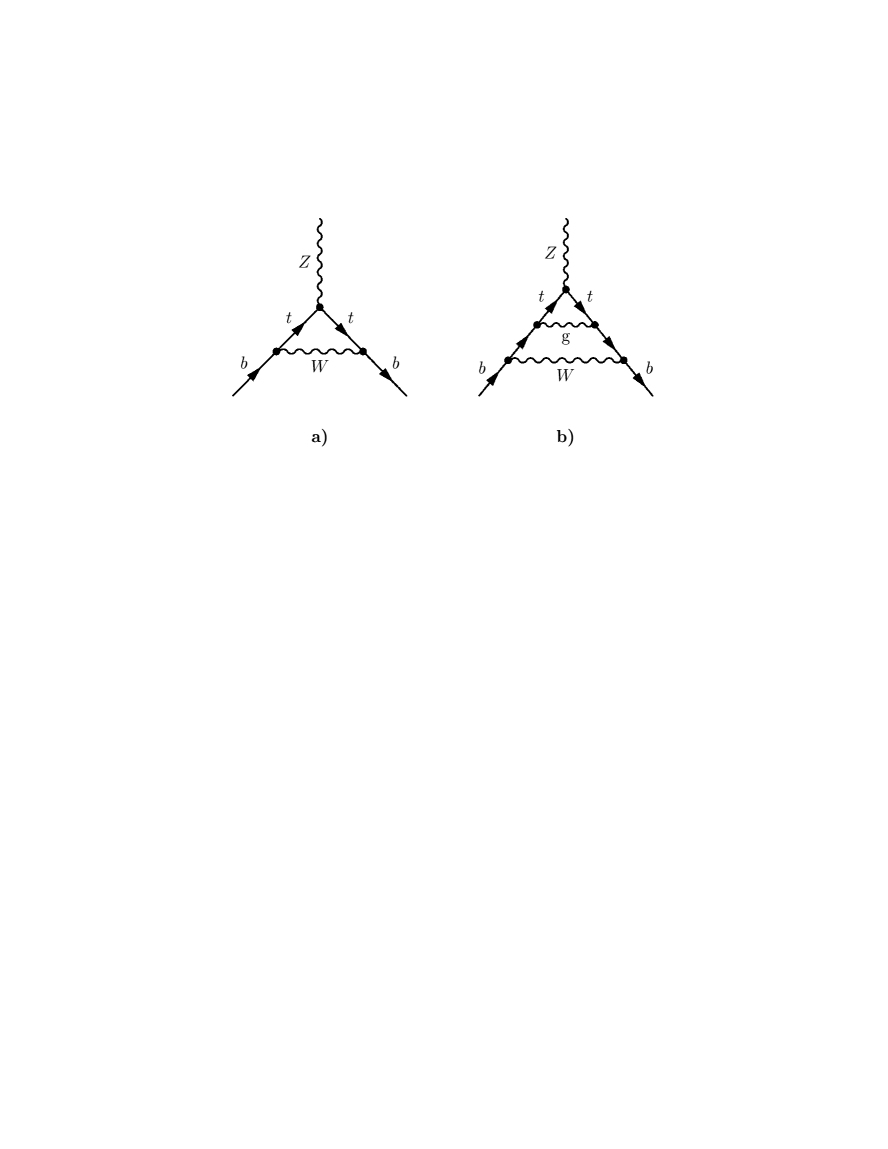
Figure 11: The vertex electroweak diagrams involving t-quark and contributing to the $Z\to b\bar{b}$ decay. Diagram (b) represents gluon corrections to diagram (a).

Here the term $\phi(t)$ calculated in [47] corresponds to a $t\bar{t}W$ vertex triangle (see Figure 11 (a)), while the term $\delta_{\alpha_{s}}\phi(t)$ calculated in [48], corresponds to the leading gluon corrections to the term $\phi(t)$ (see Figure 11 (b)): $\delta_{\alpha_{s}}\phi(t)\sim\alpha_{s}t$. Expressions for $\phi(t)$ and $\delta_{\alpha_{s}}\phi(t)$ are given in refs. [41, 42]. For $m_{t}=175$ GeV, $\hat{\alpha}_{s}(m_{Z})=0.120$

$$\phi(t)=29.96\;\;,$$ (93)

$$\delta_{\alpha_{s}}\phi(t)=-3.02\;\;,$$ (94)

and correction terms in equations (91) and (92) are very large. The subleading gluon corrections to $\phi(t)$ calculated recently [49] are very small: $\delta\Gamma_{h}(Z\to b)=-0.04$ MeV.

6 Comparison of one-electroweak-loop results and experimental LEP-I and SLC data.

6.1 LEPTOP code.

A number of computer programs (codes) were written for comparing high-precision data of LEP-I and SLC. The best known of these programs in Europe is ZFITTER [50], which takes into account not only electroweak radiative corrections but also all purely electromagnetic ones, including, among others, the emission of photons by colliding electrons and positrons. Some of the first publications in which the $t$ quark mass was predicted on the basis of precision measurements [51], were based on the code ZFITTER. Other European codes, BHM, WOH [52], TOPAZO [53], somewhat differ from ZFITTER. The best known in the USA are the results generated by the code used by Erler and Langacker [54], [23].

The original idea of the authors of this review in 1991–1993 was to derive simple analytical formulas for electroweak radiative corrections, which would make it possible to predict the $t$-quark mass using no computer codes, just by analyzing experimental data on a sheet of paper. Alas, the diversity of hadron decays of $Z$ bosons, depending on the constants of strong gluon interaction $\hat{\alpha}_{s}$, was such that it was necessary to convert analytical formulas into a computer program which we jokingly dubbed LEPTOP [55]. The LEPTOP calculates the electroweak observables in the framework of the Minimal Standard Model and fits experimental data so as to determine the quantities $m_{t}$, $m_{H}$ and $\hat{\alpha}_{s}(m_{Z})$. The logical structure of LEPTOP is clear from the preceding sections of this review and is shown in the Flowchart. The code of LEPTOP can be downloaded from the Internet home page: http://cppm.in2p3.fr./leptop/intro$\_$leptop.html

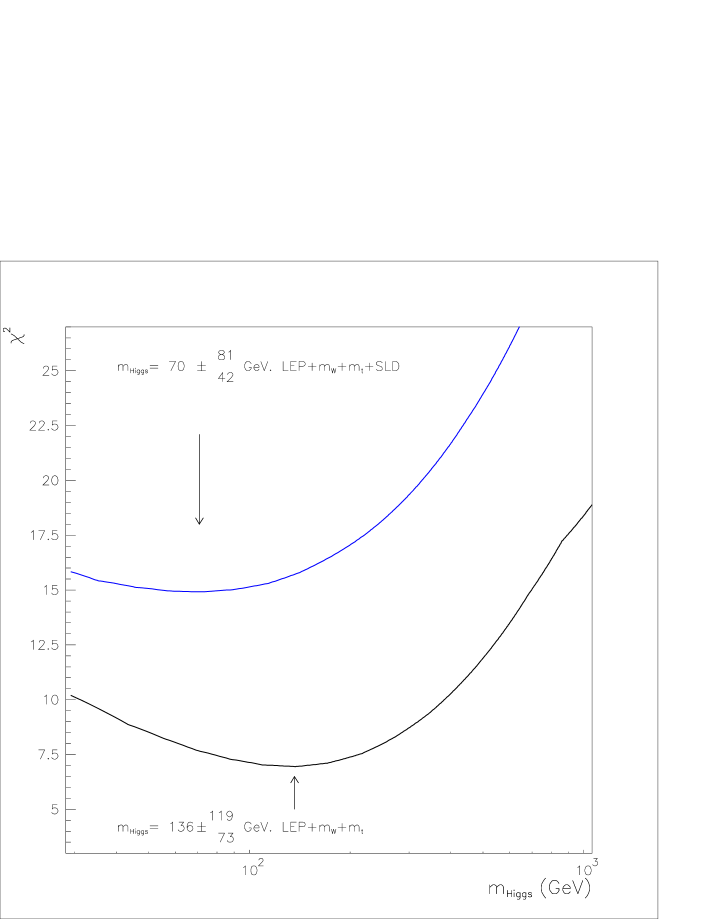
Figure 13: $\chi^{2}$ vs. $m_{H}$ curves.

A comparison of the codes ZFITTER, BHM, WOH, TOPAZO and LEPTOP carried out in 1994–95 [20] has demonstrated that their predictions for all electroweak observables coincide with accuracy that is much better than the accuracy of the experiment. The Flowcharts of LEPTOP and ZFITTER are compared on pages 25 and 27 of [20]; numerical comparison of five codes (their 1995 versions) for twelve observables is presented in figures 11-23 of the same reference. The results of processing the experimental data using LEPTOP are shown below.

6.2 One-loop general fit.

Second column of Table 4 shows experimental values of the electroweak observables, obtained by averaging the results of four LEP detectors (part a), and also SLC data (part b) and the data on $W$ boson mass (part c). (The data on the W boson mass from the $p\bar{p}$-colliders and LEP-II are also shown, for the reader’s convenience, in the form of $s^{2}_{W}$, while the data on $s_{W}^{2}$ from $\nu N$-experiments are also shown in the form of $m_{W}$. These two numbers are given in italics, emphasizing that they are not independent experimental data. The same refers to $s^{2}_{l}$ ($A_{LR}$).) We take experimental data from the paper [22]. The experimental data of Table 4 are used for determining (fitting) the parameters of the standard model in one-electroweak-loop approximation: $m_{t}$, $m_{H}$, $\hat{\alpha}_{s}(m_{Z})$ and $\bar{\alpha}$. (In fitting $m_{t}$ the direct measurements of $m_{t}$ by CDF and D0 [collaborations] [27] are also used. In fitting $\bar{\alpha}$ its value from eq.(14) was used.) The third column shows the results of the fit of electroweak observables with one loop electroweak formulas. The last column shows the value of the ‘pull’. By definition, the pull is the difference between the experimental and the theoretical values divided by experimental uncertainty. The pull values show that for most observables the discrepancy is less than $1\sigma$. The number of degrees of freedom is $18-4=14$.

Table 4. Fit of the experimental data [22] with one-electroweak-loop formulas.

$m_{Z}=91.1867(21)$ GeV is used as an input.

Output of the fit: $m_{H}=139.1^{+134.2}_{-76.5}$ GeV, $\hat{\alpha}_{s}=0.1195\pm 0.0030$, $\chi^{2}/n_{d.o.f.}=15.1/14$

	Experimental	Fit
Observable	data	standard	Pull
		model
a) LEP
shape of $Z$-peak
and lepton asymmetries:
$\Gamma_{Z}$ [GeV]	2.4939(24)	2.4959(18)	-0.8
$\sigma_{h}[nb]$	41.491(58)	41.472(16)	0.3
$R_{l}$	20.765(26)	20.747(20)	0.7
$A^{l}_{FB}$	0.0168(10)	0.0161(3)	0.8
$\tau$-polarization:
$A_{\tau}$	0.1431(45)	0.1465(14)	-0.8
$A_{e}$	0.1479(51)	0.1465(14)	0.3
Results for $b$ and $c$
quarks:
$R_{b}$∗	0.2166(7)	0.2158(2)	1
$R_{c}$∗	0.1735(44)	0.1723(1)	0.3
$A^{b}_{FB}$	0.0990(21)	0.1027(10)	-1.8
$A^{c}_{FB}$	0.0709(44)	0.0734(8)	-0.6
Charge asymmetry for pairs
of light quarks $q\bar{q}$:
$s^{2}_{l}(Q_{FB})$	0.2321(10)	0.2316(2)	0.5
b) SLC
$A_{LR}$	0.1504(23)	0.1465(14)	1.7
$s^{2}_{l}(A_{LR})$	0.2311(3)	0.2316(2)	-1.7
$R_{b}$∗	0.2166(7)	0.2158(2)	0.9
$R_{c}$∗	0.1735(44)	0.1723(1)	0.3
$A_{b}$	0.8670(350)	0.9348(1)	-1.9
$A_{c}$	0.6470(400)	0.6676(6)	-0.5
c) $p\bar{p}+$ LEP-II $+\nu N$
$m_{W}$ [GeV] $(p\bar{p})$ + LEP-II	80.39(6)	80.36(3)	0.5
	0.2228(13)
$s_{W}^{2}$ $(\nu N)$	0.2254(21)	0.2234(6)	0.9
	80.2547(1089)
$m_{t}$ [GeV]	173.8(5.0)	171.6(4.9)	0.4

^∗ Experimental values of $R_{b}$ and $R_{c}$ correspond to the average of LEP-I and SLC results.

Table 5

Observable	$s^{2}_{l}$	Average over	Cumulative	$\chi^{2}/n_{d.o.f.}$
		groups of observations	average
$A^{l}_{FB}$	0.23117(55)
$A_{\tau}$	0.23202(57)
$A_{e}$	0.23141(65)	0.23153(34)	0.23153(34)	1.2/2
$A^{b}_{FB}$	0.23226(38)
$A^{c}_{FB}$	0.23223(112)	0.23226(36)	0.23187(25)	3.4/4
$<Q_{FB}>$	0.23210(100)	0.23210(100)	0.23189(24)	3.4/5
$A_{LR}$ (SLD)	0.23109(30)	0.23109(30)	0.23157(19)	7.8/6

Table 5 gives experimental values of $s^{2}_{l}$. The third column was obtained by averaging of the second column, and the fourth by cumulative averaging of the third; it also lists the values of $\chi^{2}$ over the number of degrees of freedom.

7 Two-loop electroweak corrections and theoretical uncertainties.

In this Section we will discuss heavy top corrections of the second order in $\alpha_{W}$ to $m_{W}$ and to coupling constants of $Z$-boson with fermions. Full calculation of $\alpha_{W}^{2}$ corrections is still absent. What have been calculated are corrections of the order $\alpha_{W}^{2}$ $t^{2}=\alpha_{W}^{2}(m_{t}/m_{Z})^{4}$ [56, 57] and corrections $\sim\alpha_{W}^{2}t$ [58] - [60].

There are two sources of $\alpha_{W}^{2}t^{2}$ corrections in our approach. The first source are reducible diagrams with top quark in each loop. The second source are irreducible two-loop Feynman diagrams which contain top quark [56, 57]. We start our consideration with the first source the contribution of which is proportional to $(\Pi_{Z}(0)-\Pi_{W}(0))^{2}$. Detailed calculations are presented in Appendix F.

7.1 $\alpha_{W}^{2}t^{2}$ corrections to $m_{W}/m_{Z}\;,\;\;g_{A}$ and $g_{V}/g_{A}$ from reducible diagrams.

We start our consideration from the ratio of vector boson masses. From eq.(F.12) and (F.13) we obtain:

$$\frac{m_{W}}{m_{Z}}=c[1+\frac{c^{2}}{2(c^{2}-s^{2})}\delta+\frac{3c^{4}-10c^{4}s^{2}}{8(c^{2}-s^{2})^{3}}\delta^{2}]\;\;.$$ (95)

Substituting the expression for $\delta$ from (F.10) and using definition of $V_{m}$ eq.(47), (52) we obtain the following correction to the function $V_{m}$:

$$\delta^{\prime}_{4}V_{m}=\frac{4\pi s^{2}c^{4}(3-10s^{2})}{3\bar{\alpha}(c^{2}-s^{2})^{2}}\delta^{2}=\frac{3(3-10s^{2})\bar{\alpha}t^{2}}{64\pi s^{2}(c^{2}-s^{2})^{2}}\;\;,$$ (96)

The correction to axial coupling constant $g_{Al}$ is easily derived from equations (F.14) (since $g_{Al}\sim f_{0}$), (F.10) and definition of $V_{Al}$, equations (48), (52):

$$g_{Al}=-\frac{1}{2}-\frac{1}{4}\delta-\frac{3}{16}\delta^{2}\;\;,$$ (97)

$$\delta^{\prime}_{4}V_{A}=\frac{9\bar{\alpha}t^{2}}{64\pi s^{2}c^{2}}\;\;.$$ (98)

Finally, taking into account definition of $V_{R}$, equations (49), (52), and equations (F.15), (F.7) we get:

$$g_{Vl}/g_{Al} = 1-4[1-c^{2}-\frac{c^{2}s^{2}}{c^{2}-s^{2}}\delta+\frac{c^{4}s^{4}}{(c^{2}-s^{2})^{3}}\delta^{2}]=$$ (99)

$$= 1-4s^{2}+\frac{4c^{2}s^{2}}{c^{2}-s^{2}}\delta-\frac{4c^{4}s^{4}}{(c^{2}-s^{2})^{3}}\delta^{2}\;\;,$$

$$\delta^{\prime}_{4}V_{R}=-\frac{3\bar{\alpha}t^{2}}{16\pi(c^{2}-s^{2})^{2}}$$ (100)

Formulas (96), (98) and (100) contain corrections to the functions $V_{i}$ which come from the squares of polarization operators and are proportional to $\bar{\alpha}t^{2}$ – so, it is leading ($\sim t^{2}$) parts of $(\Pi_{Z}-\Pi_{W})^{2}$ corrections. Numerically they are several times smaller than $\bar{\alpha}t^{2}$ corrections which originate from irreducible diagrams.

7.2 $\alpha_{W}^{2}t^{2}$ corrections from irreducible diagrams.

The major part of $\alpha_{W}^{2}t^{2}$ corrections comes from the irreducible two-loop Feynman diagrams [56, 57]. The key observation in performing their calculation is that these corrections are of the order of $[\alpha_{W}(\frac{m_{t}}{m_{Z}})^{2}]^{2}\sim\lambda_{t}^{4}$, where $\lambda_{t}$ is the coupling constant of higgs doublet with the top quark. That is why they can be calculated in a theory without vector bosons, taking into account only top-higgs interactions [56]. Corresponding pieces of vector boson self-energies can be extracted from the self-energies of would-be-goldstone bosons which enter Higgs doublet (those components which after mixing with massless vector bosons form massive $W$- and $Z$-bosons). Correction of the order of $\alpha_{W}^{2}t^{2}$ is contained in the difference $\Pi_{Z}(0)-\Pi_{W}(0)$ (see Figure 12), so it is universal, i.e. one and the same for $V_{m}$, $V_{A}$ and $V_{R}$. In [42] we call these corrections $\delta_{4}V_{i}$:

$$\delta_{4}V_{i}(t,h)=-\frac{\bar{\alpha}}{16\pi s^{2}c^{2}}A(h/t)\cdot t^{2}\;\;,$$ (101)

where function $A(h/t)$ is given in the Table 6. To obtain this Table for $m_{H}/m_{t}<4$ we use a Table from the paper [57], and for $m_{H}/m_{t}>4$ we use expansion over $m_{t}/m_{H}$ from the paper [56]. For $m_{t}=175$ GeV and $m_{H}=150$ GeV we get $A=6.4$ and $\delta_{4}V_{i}(t,h)=-0.08$. This corresponds to the shifts: $-12$ MeV for $m_{W}$, $7\cdot 10^{-5}$ for $s_{l}^{2}$ and $5\cdot 10^{-5}$ for $g_{Al}$. One should compare these shifts with one-loop results: $\delta_{1{\rm loop}}m_{W}=400$ MeV, $\delta_{1{\rm loop}}s_{l}^{2}=50\cdot 10^{-5}$ and $\delta_{1{\rm loop}}g_{A}=100\cdot 10^{-5}$. Let us remind that present experimental accuracy in $m_{W}$ is $64$ MeV, in $s_{l}^{2}$ is $20\cdot 10^{-5}$ and in $g_{Al}$ is $30\cdot 10^{-5}$.

There is one more place from which corrections $\sim\alpha_{W}^{2}t^{2}$ appear: this is the $Z\to b\bar{b}$ decay. At one electroweak loop $t$-quark can propagate in the vertex triangle ($t\bar{t}W$) (see Section 5). That is why at two loops correction of the order $\alpha_{W}^{2}t^{2}$ emerges. Due to this correction functions $V_{Ab}(t,h)$ and $V_{Rb}(t,h)$ differ from the corresponding functions describing $Z\to d\bar{d}$ decay:

$$V_{Ab}(t,h)=V_{Ad}(t,h)-\frac{8s^{2}c^{2}}{3(3-2s^{2})}(\phi(t)+\delta\phi(t,h))\;\;,$$ (102)

$$V_{Rb}(t,h)=V_{Rd}(t,h)-\frac{4s^{2}(c^{2}-s^{2})}{3(3-2s^{2})}(\phi(t)+\delta\phi(t,h))\;\;,$$ (103)

where function $\phi(t)$ was discussed in Section 5 and

$$\delta\phi(t,h)=\delta_{\alpha_{s}}(t)\phi+\delta_{H}\phi(t,h)=\frac{3-2s^{2}}{2s^{2}c^{2}}\left\{-\frac{\pi^{2}}{3}(\frac{\hat{\alpha}_{s}(m_{t})}{\pi})t+\frac{1}{16s^{2}c^{2}}(\frac{\bar{\alpha}}{\pi})t^{2}\tau_{b}^{(2)}(\frac{h}{t})\right\}\;\;,$$ (104)

First term in curly braces, $\delta_{\alpha_{s}}\phi$, was taken into account earlier, see Section 5, and the new correction $\delta_{H}\phi(t,h)$ is proportional to function $\tau_{b}^{(2)}(h/t)$. Function $\tau_{b}^{(2)}$ is given in Table 6. To obtain this Table for $m_{H}/m_{t}<4$ we use a Table from the paper [57], and for $m_{H}/m_{t}>4$ we use expansion over $m_{t}/m_{H}$ from the paper [56] in full analogy with function $A(h/t)$.

For $m_{t}=175$ GeV, $m_{H}=150$ GeV we have $\tau_{b}^{(2)}=1.6$.

The change of $\Gamma_{b}$ due to $\tau_{b}^{(2)}=1.6$ equals $0.03$ MeV, which corresponds to $2\cdot 10^{-5}$ shift in $R_{b}$, while experimental accuracy in $R_{b}$ is $7\cdot 10^{-4}$ (the one e-w loop correction in $R_{b}$ is $-3.9\cdot 10^{-3}$). The influence of $\tau_{b}^{(2)}$ on $A_{FB}^{b}$ and $A_{b}$ is even smaller (by a few orders of magnitude).

Table 6: Functions $A(m_{H}/m_{t})$ and $\tau_{b}^{(2)}(m_{H}/m_{t})$.

$m_{H}/m_{t}$	$A(m_{H}/m_{t})$	$\tau_{b}^{(2)}(m_{H}/m_{t})$	$m_{H}/m_{t}$	$A(m_{H}/m_{t})$	$\tau_{b}^{(2)}(m_{H}/m_{t})$
.00	.739	5.710	2.60	10.358	1.661
.10	1.821	4.671	2.70	10.473	1.730
.20	2.704	3.901	2.80	10.581	1.801
.30	3.462	3.304	2.90	10.683	1.875
.40	4.127	2.834	3.00	10.777	1.951
.50	4.720	2.461	3.10	10.866	2.029
.60	5.254	2.163	3.20	10.949	2.109
.70	5.737	1.924	3.30	11.026	2.190
.80	6.179	1.735	3.40	11.098	2.272
.90	6.583	1.586	3.50	11.165	2.356
1.00	6.956	1.470	3.60	11.228	2.441
1.10	7.299	1.382	3.70	11.286	2.526
1.20	7.617	1.317	3.80	11.340	2.613
1.30	7.912	1.272	3.90	11.390	2.700
1.40	8.186	1.245	4.00	11.396	2.788
1.50	8.441	1.232	4.10	11.442	2.921
1.60	8.679	1.232	4.20	11.484	3.007
1.70	8.902	1.243	4.30	11.523	3.094
1.80	9.109	1.264	4.40	11.558	3.181
1.90	9.303	1.293	4.50	11.590	3.268
2.00	9.485	1.330	4.60	11.618	3.356
2.10	9.655	1.373	4.70	11.644	3.445
2.20	9.815	1.421	4.80	11.667	3.533
2.30	9.964	1.475	4.90	11.687	3.622
2.40	10.104	1.533	5.00	11.704	3.710
2.50	10.235	1.595

7.3 $\alpha_{W}^{2}t$ corrections and the two-loop fit of experimental data.

Corrections of the order $\alpha_{W}^{2}t$ originate from the top loop contribution to $W$- and $Z$-boson self-energies with higgs or vector boson propagating inside the loop and are of the order of $g^{2}\lambda_{t}^{2}$. We take into account these corrections in our code LEPTOP using results of the papers [58] - [60].

Before we will present results of electroweak precision data fit which take into account $\alpha_{W}^{2}$ corrections, described in this Section, we must discuss how good the approximation which takes into account $\alpha_{W}^{2}t^{2}$ and $\alpha_{W}^{2}t$ terms but neglects (still not calculated) $\alpha_{W}^{2}$ terms should be. For $m_{t}=175$ GeV we obtain $t\simeq 3.7$, thus at first glance we have good expansion parameter so that $\alpha_{W}^{2}$ terms could be safely neglected. To check this let us consider first the one electroweak loop, where the enhanced $\alpha_{W}t$ terms can be compared with non-enhanced $\alpha_{W}$ terms.

By using eqs.(47) and (49) and by comparing them with experimental data one sees that for $m_{W}/m_{Z}$ the $\alpha_{W}t$ term is equal to $0.0057$, while the $\alpha_{W}$ term is $-0.0014$. As for $g_{Vl}/g_{Al}$, the two terms are $0.0122$ and $-0.0142$. Thus for $m_{W}/m_{Z}$ the $\alpha_{W}t$ term dominates, while for $g_{Vl}/g_{Al}$ it is practically cancelled by the $\alpha_{W}$ term.

Coming back to two-loop corrections we observe, that $\alpha_{W}^{2}t^{2}$ correction to $m_{W}$ is not larger than $\alpha_{W}^{2}t$ correction; for $m_{t}=175$ GeV and $m_{H}=150$ GeV it diminishes $m_{W}$ by $23$ MeV (compare with Section 7.2).

In the Table 7 we present results of the fit of the data where we use theoretical formulas which include two-loop electroweak corrections described in this Section. Comparing Table 7 with Table 4 where the fit of the one-loop electroweak corrected formulas was presented, we see that the fitted values of all physical observables are practically the same with one (very important) exception: the central value of the higgs mass becomes $\sim 70$ GeV lower. In view of the previous discussion it seems reasonable to consider this shift as a cautious estimate of the theoretical uncertainty in $m_{H}$.

We have a simple qualitative explanation why $\alpha_{W}^{2}t$ corrections reduce the higgs mass by $\sim 70$ GeV. The point is that these corrections shift the theoretical value of $s_{l}^{2}$ by $+0.0002$, which is close to experimental error in $s_{l}^{2}$. In order to compensate the shift the fitted mass of the higgs changes. This change can be easily derived. Indeed, from eqs.(49), (52), (45) we get:

$$\delta s^{2}=-\frac{3}{16\pi(c^{2}-s^{2})}\bar{\alpha}\delta H_{R}=-0.00086\delta H_{R}\;\;,$$ (105)

while from Table 3 we see that changing $m_{H}$ from $150$ GeV to $100$ GeV gives $\delta H_{R}=+0.236$ and $\delta s^{2}=-0.0002$.

In Figure 13 the dependence of $\chi^{2}$ on the value of higgs mass is shown separately with and without inclusion of SLD data ($Z$-decays into heavy quark pairs are taken into account on both plots). When all existing data are taken into account we get central value of higgs mass $m_{H}=71$ GeV which is twenty GeV below direct bound [22] from LEP-II search: $m_{H}>95$ GeV. However, uncertainty in the value of $m_{H}$ extracted from radiative corrections is quite large, thus there is no contradiction between these two numbers.

At the end of this Section we would like to make two remarks demonstrating that one should not take too seriously the central values of $m_{H}$ extracted from the global fits.

First, if one disregards the FNAL measurements of $m_{t}$, then one obtains from the fit:

$$m_{t}=160.7^{+7.7}_{-6.8}\;\mbox{\rm GeV}\;\;,$$

$$m_{H}=30.3^{+38.8}_{-14.4}\;\mbox{\rm GeV}\;\;.$$

Such value of $m_{H}$ is by 1.5 standard deviations below the lower bound from direct searches of LEP-II.( Note also that the fitted value of the top mass $m_{t}$ is substantially lower than measured at FNAL).

Second, as it was stressed in ref. [61], the values of $s_{l}^{2}$ extracted from different observables lead to very different central values of $m_{H}$. For example, from SLAC data on $A_{LR}$ it follows that $m_{H}=25$ GeV with 90% confidence interval from $6$ GeV to $100$ GeV. Even smaller values of $m_{H}$ follow from LEP measurement of $A_{FB}^{\tau}$: $m_{H}=4$ GeV ($0.2$ GeV $<m_{H}<95$ GeV at 90% C.L.). As for other asymmetries measured at LEP, they lead to much heavier higgs: from $A_{FB}^{b}$, for example, $m_{H}=370$ GeV ($100$ GeV $<m_{H}<1400$ GeV at 90% C.L.). That is why the average of all these values of $m_{H}$ seems to be not very reliable.

Table 7. Fit of experimental data [22] with two-electroweak-loop formulas.

$m_{Z}=91.1867(21)$ GeV is used as an input.

Output of the fit: $m_{H}=70.8^{+82}_{-43}$ GeV^∗, $\hat{\alpha}_{s}=0.1194\pm 0.0029$, $\chi^{2}/n_{d.o.f.}=15.0/14$

Observable	Experimental	Fit Standard	Pull
	data	Model
a) LEP-I
shape of $Z$-peak and
lepton asymmetries:
$\Gamma_{Z}$ [GeV]	2.4939(24)	2.4960(18)	-0.9
$\sigma_{h}$ [nb]	41.491(58)	41.472(16)	0.3
$R_{l}$	20.765(26)	20.746(20)	0.7
$A_{FB}^{l}$	0.0168(10)	0.0161(4)	0.7
$\tau$-polarization:
$A_{\tau}$	0.1431(45)	0.1467(16)	-0.8
$A_{e}$	0.1479(51)	0.1467(16)	0.2
results for heavy quarks:
$R_{b}$∗∗	0.2166(7)	0.2158(2)	1.0
$R_{c}$∗∗	0.1735(44)	0.1723(1)	0.3
$A_{FB}^{b}$	0.0990(21)	0.1028(12)	-1.8
$A_{FB}^{c}$	0.0709(44)	0.0734(9)	-0.6
charge asymmetry for pairs of
light quarks $q\bar{q}$:
$s_{l}^{2}(Q_{FB})$	0.2321(10)	0.2316(2)	0.5
b) SLC
$s_{l}^{2}$ ($A_{LR}$)	0.2311(3)	0.2316(2)	-1.6
$A_{LR}$	0.1504(23)	0.1467(16)	1.6
$R_{b}$∗∗	0.2166(7)	0.2158(2)	0.9
$R_{c}$∗∗	0.1735(44)	0.1723(1)	0.3
$A_{b}$	0.8670(350)	0.9348(2)	-1.9
$A_{c}$	0.6470(400)	0.6677(7)	-0.5
c) $p\bar{p}+$ LEP-II $+\nu N$
$m_{W}$ [GeV] ($p\bar{p}+$ LEP-II)	80.3902(64)	80.3659(34)	0.4
	0.2228(13)
$s_{W}^{2}$ ($\nu N$)	0.2254(21)	0.2233(7)	1.0
	80.255(109)
$m_{t}$ [GeV]	173.8(5.0)	170.8(4.9)	0.6

^∗ The most optimistic errors on $M_{H}$ are obtained in the fit including $\bar{\alpha}(DH)^{-1}=128.923(36)$ [30] and $\alpha_{s}(PDG)=0.1178(23)$ from low energy data [27]. Such a fit gives $m_{H}=93^{+63}_{-41}$ GeV, $m_{t}=171.3\pm 4.8$ GeV, $\alpha_{s}=0.1184\pm 0.0018$, $\chi^{2}/n_{d.o.f.}=15.2/14$. However the systematic errors due to the model assumptions used in the calculations of $\alpha_{s}(PDG)$ and $\bar{\alpha}(DH)$ are not easy to estimate. That is why we prefer to use the result with less optimistic assumptions leading to bigger error in $m_{H}$.
^∗∗ Experimental values of $R_{b}$ and $R_{c}$ correspond to the average of LEP-I and SLC results.

As can be seen from the Table 8, the LEPTOP fit is very close to the ZFITTER fit [22] and to the fit by Erler and Langacker [23]. This indicates that theoretical uncertainties are very small, except for the non-calculated part of the corrections, that is common to all three programs.

Table 8. Comparison of the LEPTOP fit with the ZFITTER fit [22] and with the fit by Erler and Langacker [23].

Observable	Experimental	Fit LEPTOP	Fit EWWG	Fit Erler-
	data		ZFITTER	Langacker∗
a) LEP-I
$M_{Z}$ [GeV]	91.1867(21)	91.1867 fix.	91.1865	91.1865(21)
$\Gamma_{Z}$ [GeV]	2.4939(24)	2.4960(18)	2.4958	2.4957(17)
$\sigma_{h}$ [nb]	41.491(58)	41.472(16)	41.473	41.473(15)
$R_{l}$	20.765(26)	20.746(20)	20.748	20.748(19)
$A_{FB}^{l}$	0.0168(10)	0.0161(4)	0.01613	0.0161(3)
$A_{\tau}$	0.1431(45)	0.1467(16)	0.1467	0.1466(15)
$A_{e}$	0.1479(51)	0.1467(16)	0.1467	0.1466(13)
$R_{b}$	0.2166(7)	0.2158(2)	0.2159	0.2158(2)
$R_{c}$	0.1735(44)	0.1723(1)	0.1722	0.1723(1)
$A_{FB}^{b}$	0.0990(21)	0.1028(12)	0.1028	0.1028(10)
$A_{FB}^{c}$	0.0709(44)	0.0734(9)	0.0734	0.0734(8)
$s_{l}^{2}(Q_{FB})$	0.2321(10)	0.2316(2)	0.23157	0.2316(2)
b) SLC
$s_{l}^{2}$($A_{LR}$)	0.2311(3)	0.2316(2)	0.23157	–
$A_{LR}$	0.1504(23)	0.1467(16)	—	0.1466(15)
$A_{b}$	0.8670(350)	0.9348(2)	0.935	0.9347(1)
$A_{c}$	0.6470(400)	0.6677(7)	0.668	0.6676(6)
c) $p\bar{p}+$ LEP-II $+\nu N$
$m_{W}$ [GeV] ($p\bar{p}+$ LEP-II)	80.3902(64)	80.3659(34)	80.37	80.362(23)
	0.2228(13)
$s_{W}^{2}$ ($\nu N$)	0.2254(21)	0.2233(7)	0.2232
	80.255(109)
$m_{t}$ [GeV]	173.8(5.0)	170.8(4.9)	171.1(4.9)	171.4(4.8)
$m_{H}$ [GeV]		$71.^{+82}_{-43}$	$76.^{+85}_{-47}$	$107.^{+67}_{-45}$
$\alpha_{s}$		0.1194(29)	0.119(3)	0.1206(30)
$\bar{\alpha}^{-1}$	128.878(90)	128.875	128.878

^∗ Erler-Langacker use slightly different experimental dataset for their fit. This may cause some of the discrepancies with LEPTOP and ZFITTER.

8 Extensions of the Standard Model.

The Standard Model works well at the energy scale of the order of the vector bosons masses. We see that the SM description of the electroweak observables in this energy region is in perfect agreement with the precision measurements.

However there are many natural physical questions that have no satisfactory answers within the framework of the SM. So it is hard to believe that the Standard Model is the Final Theory. The common expectation is that there should be New Physics beyond the Standard Model.

Direct accelerator searches did not find yet any trace of New Physics. Their negative results gave lower bounds on the masses and upper bounds on the production cross sections for the new particles. In this section we are going to study the indirect bounds on New Physics that can be theoretically derived from the precision measurements at low energy of the order of $Z$ and $W$ boson masses. Loops with hypothetical new particles change the predictions of the SM for electroweak observables. Since the SM gives a very good description of the data there is little room for such new contributions. In this way one can get some kind of constraints on new theory.

Any possible generalizations of the SM are naturally divided into two classes: theories with and without decoupling. In the first class the contribution of new particles into $W$ and $Z$ boson parameters are suppressed as positive powers of $(m_{Z}^{2}/m^{2})^{n}$ when the masses of new particles $m$ become larger than electroweak scale. One cannot exclude such theory by studying loop corrections to low-energy observables. In this way one may have hopes to bound the masses of new particles from below. The most famous example of such theory are supersymmetric extensions of the SM.

In the second class of theories the contribution of new particles into low-energy observables does not decouple even when their masses become very large. Such SM generalizations can be excluded if the additional nondecoupled contributions exceed the discrepancy between SM fit and experimental data. The example of such generalization is the SM with additional sequential generations of quarks and leptons.

8.1 Sequential heavy generations in the Standard Model.

We start the discussion of New Physics with the simplest extension of the SM, namely with the SM with additional sequential generations of leptons and quarks ([62]- [64]). Nobody knows any deep reason for the number of generations to be equal to three. So it is interesting to study whether it is allowed to have four and more generations. Certainly these new generations should be heavy enough not to be produced in the $Z$ decays and at LEP-II.

We consider the case of no mixing between the known generations and the new ones. In this case the new fermion generations affect the ratio $m_{W}/m_{Z}$ and the widths and the decay asymmetries of the $Z$ boson only through the vector bosons self-energies. Such kind of corrections have been dubbed [88] ”oblique corrections”. We start their study with the case of $SU(2)$ degenerate fourth generation:

$$m_{U}=m_{D}=m_{Q}\;\;,\quad\quad m_{N}=m_{E}=m_{L}$$ (106)

New terms in the self-energies modify the functions $V_{m},V_{A},V_{R}$ , i.e. the radiative corrections to $m_{W}/m_{Z}$, $g_{Al}$ and $g_{Vl}/g_{Al}$. The contribution to $V_{i}$ from the fourth generation can be written in the form:

$$V_{m}\to V_{m}+\delta^{4}V_{m}\;,\;\;V_{A}\to V_{A}+\delta^{4}V_{A}\;,\;\;V_{R}\to V_{R}+\delta^{4}V_{R}\;\;.$$ (107)

The analytical expressions for $\delta^{4}V_{i}$ for quark or lepton doublets (neglecting gluonic corrections) can be found in Appendix G, eqs (G.1)-(G.3).

In the limit of a very heavy fourth generation of leptons and quarks one has :

$$\Sigma\delta^{4}V_{m}\to-\frac{16}{9}s^{2}\;,\;\;\Sigma\delta^{4}V_{R}\to-\frac{8}{9}\;,\;\;\Sigma\delta^{4}V_{A}\to 0\;\;,$$ (108)

where $\Sigma$ denotes sum over leptons and quarks with $m_{Q}=m_{L}=m_{4}$, $s^{2}\simeq 0.23$. Equations (108) reflect the non-decoupling of the heavy degrees of freedom in electroweak theory, caused by the axial current. It is interesting that the contribution of degenerate generation to $V_{m},V_{R}$ has negative sign.

The fourth generation with strong violation of $SU(2)$ symmetry (i.e. with very large mass difference in the doublet) gives universal contribution to functions $\delta^{4}V_{i}$ (similar to the universal contribution of $t$- and $b$-quarks from the third generation to $V_{i}$)

$$\delta^{4}V_{i}=4|m^{2}_{T}-m^{2}_{B}|/3m^{2}_{Z}.$$ (109)

In the case of large mass splitting $\delta^{4}V_{i}$ are positive. From eqs.(108) and (109) it is clear that somewhere in the intermediate region of mass splitting the functions $\delta^{4}V_{m}$ and $\delta^{4}V_{R}$ intersect zero. In the vicinities of these zeroes the contribution of new generation to these specific observables is negligible and one can not exclude these regions of masses studying only one of the observables. Fortunately for different observables these zeroes are located in the different places and the general fit overcomes such conspiracy of new physics.

For different up- and down- quark (and lepton) masses analytical expressions for $\delta^{4}V_{i}$ are given in Appendix G, eqs.(G.4) - (G.6).

Figure 14 demonstrates 2-dimensional exclusion plot for the case of $n$ extra generations, where $n$ is formally considered as a continuous parameter. We see from this plot that at 90% c.l. we have less than one extra generation and at 99% c.l.– less than two extra generations for any differences of up- and down- quarks masses.

8.2 SUSY extensions of the Standard Model.

In this section we consider another example of new physics: supersymmetric extensions of the SM. There are certain aesthetic and conceptual merits of such SUSY generalization of the SM. Here are some of them:

1) Supersymmetry gives a solution for the problem of fine tuning, i.e. it prevents the electroweak scale of the SM from mixing with the Planck scale.

2) The problem of unification of electroweak and strong coupling constants seems to have solution in the framework of SUSY extensions.

3) Finally, any ambitious ”Theory of Everything” inevitably includes SUSY as the basic element of the construction.

To make systematic introduction into SUSY extensions of the SM one needs a separate review paper ( for the review papers see e.g. [65] ). Here we are going to make a short sketch of this well developed branch of physics in applications to the theory of $Z$ boson. To construct SUSY extensions one has to introduce a lot of new particles. For example minimal $N=1$ supersymmetry automatically doubles the number of degrees of freedom of the SM: any fermionic degree of freedom has to be coupled with bosonic degree of freedom and vice versa. Thus the left ( right ) leptons have to be accompanied by scalars: “left” (“right” ) sleptons, quarks by squarks, gauge bosons by spinor particles – gauginos, etc. The Higgs mechanism of mass generation for up and down quarks requests for two Higgs boson doublets ( and two higgsino doublets respectively).

Not a one of these numerous new particles has been observed yet. If they do exist they are too heavy to be produced at the working accelerators. On the other hand, these heavy supersymmetric particles (again if they do exist) are produced in the virtual states, i.e. in the loops. Loops with new particles change the predictions of the SM for the low-energy observables. ( Under “low-energy” we mean here $E\mathrel{\mathchoice{\lower 3.6pt\vbox{\halign{$\mathsurround=0pt\displaystyle\hfil#\hfil$\cr<\crcr\sim\crcr}}}{\lower 3.6pt\vbox{\halign{$\mathsurround=0pt\textstyle\hfil#\hfil$\cr<\crcr\sim\crcr}}}{\lower 3.6pt\vbox{\halign{$\mathsurround=0pt\scriptstyle\hfil#\hfil$\cr<\crcr\sim\crcr}}}{\lower 3.6pt\vbox{\halign{$\mathsurround=0pt\scriptscriptstyle\hfil#\hfil$\cr<\crcr\sim\crcr}}}}m_{Z}$ ). In this indirect way one can get some information about existence or nonexistence of SUSY.

The SUSY extensions of the SM belong to the class of new physics that decouples from the low-energy observables when the mass scale of this new physics becomes very large. It means that the additional contribution into electroweak observables due to the supersymmetric particles are of the order of $\alpha_{W}(m_{W}/m_{SUSY})^{2}$ or $\alpha_{W}(m_{t}/m_{SUSY})^{2}$ , where $m_{SUSY}$ characterizes the mass scale of superpartners. Since the fit of the precision data in the framework of the SM statistically is very good these new additional contributions have to be small. So in this way one expects to get strong restrictions on the value of $m_{SUSY}$.

Supersymmetric contributions into low-energy observables were studied in papers [66] - [69]. The results depend on the model and on the pattern of SUSY violation. Within a given model the results for low-energy observables are formulated in terms of the functions that depend on the fundamental parameters of the SUSY Lagrangian that are fixed at the high energy scale of SUSY violation. The fit of experimental data in the framework of a given SUSY model imposes certain restrictions on the allowed region of these high-energy scale parameters of the model. As for the masses of sparticles their values are calculated by numerical solution of the renormalization group equations. They also depend on the fundamental SUSY parameters at high energy scale. In this rather indirect way one gets restrictions on the physical masses of sparticles in general case.

To give the reader the taste of exploration of the new supersymmetric physics we consider in this section only that part of the multi-dimensional space of SUSY parameters for which all sparticles have more or less the same masses, i.e. when we have no light sparticles. (It seems reasonable to start the study of the unknown field with such kind of the simplest assumptions). In this case one can find the class of enhanced oblique corrections that are universal, i.e. that are the same for any model. Another merit of these corrections is that they directly depend on the masses of sparticles.

As will be shown, the enhanced electroweak radiative SUSY corrections are induced by the large violation of $SU(2)_{L}$ symmetry in the third generation of squarks. Therefore we start the discussion of the SUSY corrections to the functions $V_{i}$ with the brief description of the stop $(\tilde{t}_{L},\tilde{t}_{R})$ and sbottom $(\tilde{b}_{L},\tilde{b}_{R})$ sector of the theory. The following relation between masses of quarks $q$ and diagonal masses of left squarks $\tilde{q}_{L}$ takes place in a wide class of SUSY models:

$$m^{2}_{\tilde{q}_{L}}=m_{q}^{2}+m_{SUSY}^{2}+m_{Z}^{2}\cos(2\beta)(T_{3}-s^{2}Q_{q})\;\;,$$ (110)

where $s^{2}\simeq 0.23$, $Q_{q}$ is the charge and $T_{3}$ is the third projection of weak isospin of quark and ${\rm tg}\beta$ is equal to the ratio of the vevs of two Higgs fields, introduced in SUSY models. The second term in the r.h.s of the eq.(110) violates supersymmetry. It is some universal SU(2)-blind SUSY violating soft mass term. The third term in r.h.s of the eq.(110) also violates SUSY. It originates from quartic $D$ term in the effective potential and is different for $up$ and $down$ components of the doublets. The only hypothesis that is behind this relation is that the origin of the large breaking of this $SU(2)_{L}$ is in the quark-higgs interaction.

Therefore from eq.(110) we get the following relation between masses of stop $m^{2}_{\tilde{t}_{L}}$, of sbottom $m^{2}_{\tilde{b}_{L}}$ and of top $m^{2}_{t}$ ( we neglect $m_{b}$ ):

$$m^{2}_{\tilde{t}_{L}}-m^{2}_{\tilde{b}_{L}}=m_{t}^{2}+m_{Z}^{2}\cos(2\beta)c^{2}\;\;,$$ (111)

Relation (111) is central for this approach. It demonstrates the large violation of $SU(2)_{L}$ symmetry in the third generation of squarks. On the other hand it demonstrates that in the limit of very large mass the left stop and left sbottom become degenerate and the parameter $(m^{2}_{\tilde{t}_{L}}-m^{2}_{\tilde{b}_{L}})/m^{2}_{\tilde{b}_{L}}$ goes to zero when $m_{SUSY}$ goes to infinity. That is why the physical observables can depend on this decoupling parameter.

As for the right sparticles from the third generation, they are $SU(2)_{L}$ singlets. But they can mix with the left sparticles and in this way they contribute into enhanced corrections. The mixing between $\tilde{b}_{L},\tilde{b}_{R}$ has to be proportional to $m_{b}$ and can be neglected. The $\tilde{t}_{L}\tilde{t}_{R}$ mass matrix in general has the following form:

$$\left(\begin{array}[]{cc}m^{2}_{\tilde{t}_{L}}&m_{t}A^{\prime}_{t}\\ m_{t}A^{\prime}_{t}&m^{2}_{\tilde{t}_{R}}\end{array}\right)\;\;,$$ (112)

where $\tilde{t}_{L}\tilde{t}_{R}$ mixing is proportional to $m_{t}$ and therefore is not small. Coefficient $A^{\prime}_{t}$ depends on the model. Diagonalizing matrix (112) we get the following eigenstates:

$$\left\{\begin{array}[]{l}\tilde{t}_{1}=c_{u}\tilde{t}_{L}+s_{u}\tilde{t}_{R}\\ \tilde{t}_{2}=-s_{u}\tilde{t}_{L}+c_{u}\tilde{t}_{R}\;\;,\end{array}\right.$$ (113)

where $c_{u}\equiv\cos\theta_{LR}$, $s_{u}\equiv\sin\theta_{LR}$, $\theta_{LR}$ is the $\tilde{t}_{L}\tilde{t}_{R}$ mixing angle, and

$${\rm tg}^{2}\theta_{LR}=\frac{m_{1}^{2}-m_{\tilde{t}_{L}}^{2}}{m_{\tilde{t}_{L}}^{2}-m_{2}^{2}}\;\;,\;\;m_{1}^{2}\geq m_{\tilde{t}_{L}}^{2}\geq m_{2}^{2}\;\;.$$ (114)

Parameters $m_{1}$ and $m_{2}$ are the mass eigenvalues:

$$m_{1,2}^{2}=\frac{m^{2}_{\tilde{t}_{L}}+m^{2}_{\tilde{t}_{R}}}{2}\pm\frac{|m^{2}_{\tilde{t}_{L}}-m^{2}_{\tilde{t}_{R}}|}{2}\sqrt{1+\frac{4m_{t}^{2}A^{\prime 2}_{t}}{(m^{2}_{\tilde{t}_{L}}-m^{2}_{\tilde{t}_{R}})^{2}}}\;\;.$$ (115)

The enhanced electroweak radiative corrections are induced by the contribution of the third generation of squarks into self-energy operators of vector bosons. Nondiagonal vector currents of squarks are not conserved only because of violation of SU(2) by mass terms. Thus one should expect that the self-energy operators are proportional to the divergency of the currents. To calculate these enhanced terms it is sufficient to expand the operators of the vector bosons $\Sigma_{V}(k^{2})$ at $k^{2}=0$. The terms enhanced as $m_{t}^{4}/M_{SUSY}^{2}$ come from $\Sigma_{W}(0)$, while those enhanced as $m_{t}^{2}M_{W}^{2}/M_{SUSY}^{2}$ come from $\Sigma^{\prime}_{W,Z}(0)$ (see Figure 15). These simple self-energy corrections are obviously universal since stop and sbottom should exist in any SUSY model and the coupling constants are universal since they are fixed by gauge invariance only. The higher-order derivatives of self energies are suppressed as $(m_{W,Z}/m_{SUSY})^{2}$. They are of the same order of magnitude as the numerous model-dependent terms coming from vertex and box diagrams. If there are no very light sparticles the first two universal terms have rather large enhancement factor of the order of $t^{2}\simeq 14$ and $t\simeq 3.7$ respectively.(The presence of terms $\sim m_{t}^{4}$ in SUSY models was recognized long ago [70] ). We neglect the non-enhanced terms. The accuracy of such approximation may be of the order of ten percent if we are lucky, but it may be as well of the order of unity (see discussion of $V_{R}$ in Sections 5 and of the two-loop corrections in Section 7). As for the stop contributions to the vertex corrections there is only one relevant case - the amplitude of $Z\to b\bar{b}$ decay. For vertex with stop exchange there are no terms enhanced as $(m_{t}/m_{W})^{4}$ [71]. Thus we will neglect corresponding corrections as well.

The calculation of the enhanced two terms is a rather trivial exercise. The only subtle point is the diagonalization of the stop propagators. The result of calculations depends on 3 parameters: $m_{1}$, $m_{2}$ and $m_{\tilde{b}_{L}}$. The dependence on angle $\beta$ is very moderate and in numerical fits we will use rather popular value ${\rm tg}\beta=2$. In what follows instead of $m_{\tilde{b}_{L}}$ we will write $m_{\tilde{b}}$, bearing in mind that $\tilde{b}_{L}\tilde{b}_{R}$ mixing is proportional to $m_{b}$ and can be neglected. The formulas that describe the enhanced SUSY corrections to the functions $V_{i}$ can be found in the Appendix G, eqs.(G.7) - (9).

There is also another source of the potentially large SUSY corrections: vertices with gluino exchange of the order $\hat{\alpha}_{s}(m_{Z}/m_{SUSY})^{2}$.

These corrections shift the radiators $R_{V_{q}}$ and $R_{A_{q}}$ in eq.(31) [73]:

$$\delta R_{V_{q}}=\delta R_{A_{q}}=1+\frac{\hat{\alpha}_{s}(m_{Z})}{\pi}\Delta_{1}(x,y)\;\;,$$ (116)

$$\Delta_{1}(x,y)=-\frac{4}{3}\int\limits_{0}^{1}dz_{1}\int\limits_{0}^{1-z_{1}}dz_{2}\log[1-\frac{xyz_{1}z_{2}}{x+(z_{1}+z_{2})(y-x)}]\;\;,$$ (117)

where $x=(m_{Z}/m_{\tilde{q}})^{2}$, $y=(m_{Z}/m_{\tilde{g}})^{2}$, and $\Delta_{1}(x,x)\simeq\frac{1}{18}x+...$. We take these gluino corrections into account in our analysis. The electroweak SUSY corrections to $g_{A_{q}}$ and $g_{V_{q}}$ are generated by the corrections to the function $V_{A}$ eq.(G.7) and $V_{R}$ eq.(G.8).

Having all the necessary formulas in hands we start the new fit of the data with the simplest case of the absence of $\tilde{t}_{L}\tilde{t}_{R}$ mixing, $\sin\theta_{LR}=0$. In this case we have only one additional mass parameter. Thus we expect that this mass should be heavy enough not to destroy the perfect SM fit of the experimental data. First let us take the value of the lightest neutral Higgs boson mass as a free parameter and take the masses of the other three Higgs bosons to be very heavy. The results of the fit are shown in Table 9. We see that to fit the data with light sbottom one has to take the mass of the Higgs boson much larger than its Standard Model fit value. Even in this case the quality of the fit is worse than the SM one. For very heavy sbottom one reproduces the SM fit. (To reduce the number of parameters we take $m_{\tilde{g}}=m_{\tilde{b}}$ in this fit. Let us stress that light squarks with masses of the order of $100-200$ GeV are usually allowed only if gluinos are heavy, $m_{\tilde{g}}\geq 500$ GeV [74]. In the case of heavy gluino the correction $\Delta_{1}$ (eq. (117)) becomes power suppressed and we return to the Standard Model fit value of $\hat{\alpha}_{s}=0.119(3)$).

Table 9

$m_{\tilde{b}}$ (GeV)	$m_{h}$ (GeV)	$\hat{\alpha}_{s}$	$\chi^{2}/n_{d.o.f.}$
100	$850^{+286}_{-320}$	$0.113\pm 0.003$	20.3/14
150	$484^{+364}_{-235}$	$0.116\pm 0.003$	18.1/14
200	$280^{+240}_{-144}$	$0.117\pm 0.003$	17.3/14
300	$152^{+145}_{-87}$	$0.118\pm 0.003$	16.3/14
400	$113^{+115}_{-68}$	$0.119\pm 0.003$	15.8/14
1000	$77^{+87}_{-47}$	$0.119\pm 0.003$	15.2/14

Fit of the precision data with SUSY corrections taken into account in the case of the absence of $\tilde{t}_{L}\tilde{t}_{R}$ mixing, $\sin\theta_{LR}=0$ and $m_{h}$ taken as a free parameter. For $m_{\tilde{b}}>300$ GeV SUSY corrections become negligible and SM fit of the data is reproduced.

We see that to get reasonably good fit of the data in the framework of the SUSY extensions with light squarks one has to put the lightest Higgs mass in the TeV region. It is time to remind that in SUSY models the mass of Higgs boson is not an absolutely free parameter. In MSSM (Minimal Supersymmetric Standard Model) among three neutral Higgs bosons the lightest one should have mass less than approximately $120-135$ GeV [76]. If other higgses are considerably heavier the lightest scalar boson has the same couplings with gauge bosons as in the Standard Model. As a result the same SM formulas for radiative corrections can be used in the SUSY extensions of the SM. (Deviations from the SM formulas are suppressed as $(m_{h}/m_{A})^{2}$, where $m_{A}$ – the mass of the heavier higgs. We will assume in our analysis that $m_{A}$ is large). For maximal allowed value $m_{h}\simeq 120$ GeV the results of the fit are shown in Table 10. (In what follows we will always take $m_{h}\simeq 120$ GeV since for $90$ GeV $<m_{h}<135$ GeV results of the fit are practically the same.) This table demonstrates that superpartners should be heavy if we want to have good quality fit of the data.

Table 10

$m_{\tilde{b}}$ (GeV)	$\hat{\alpha}_{s}$	$\chi^{2}/n_{d.o.f.}$
100	$0.110\pm 0.003$	30.2/15
150	$0.115\pm 0.003$	21.9/15
200	$0.116\pm 0.003$	18.6/15
300	$0.118\pm 0.003$	16.4/15
400	$0.119\pm 0.003$	15.8/15
1000	$0.119\pm 0.003$	15.5/15

The same as Table 9 but with the value of the lightest Higgs boson mass $m_{h}=120$ GeV which is about the maximum allowed value in the simplest SUSY models.

The next step is to take into account $\tilde{t}_{L}\tilde{t}_{R}$ mixing. In the Figure 16 we show the dependence of SUSY corrections $\delta_{SUSY}V_{i}$ on $m_{1}$ and $m_{2}$ for $m_{\tilde{b}}=200$ GeV. One clearly sees from this Figure that even for this small value of $m_{\tilde{b}}$ there exist the domain of low $m_{2}$ values where the enhanced radiative corrections are suppressed. In Figure 16 one sees the valley where $\delta_{SUSY}V_{i}$ reaches its minimum values which are considerably smaller than 1. The valley starts at $m_{2}\simeq m_{\tilde{b}}$, $m_{1}\simeq 1000$ GeV and goes to $m_{2}\simeq 100$ GeV, $m_{1}\simeq 400$ GeV. The smallness of the radiative corrections at the point $m_{2}\simeq m_{\tilde{b}}$, $m_{1}\simeq 1000$ GeV can be easily understood: here $\theta_{LR}\simeq\pi/2$, $\tilde{t}_{2}\simeq\tilde{t}_{L}$, $\tilde{t}_{1}\simeq\tilde{t}_{R}$. Thus nondiagonal charged left current of squarks is conserved and the main enhanced term vanishes. Indeed in $\delta_{SUSY}V_{A}$ only the term proportional to $g(m_{2},m_{\tilde{b}})$ remains in eq.(G.7), but for $m_{2}=m_{\tilde{b}}$ it is equal to zero. At this end point of the valley $\tilde{t}_{2}\simeq\tilde{t}_{L}$, $\tilde{t}_{1}\simeq\tilde{t}_{R}$, so $m^{2}_{\tilde{t}_{R}}\gg m^{2}_{\tilde{t}_{L}}$, which is opposite to the relation between $m_{\tilde{t}_{R}}$ and $m_{\tilde{t}_{L}}$ occurring in a wide class of models. In these models (e.g. in the MSSM) the left and the right squark masses are equal at high energy scale. When renormalizing them to low energies one gets $m^{2}_{\tilde{t}_{L}}>m^{2}_{\tilde{t}_{R}}$. Almost along the whole valley we have ${\rm tg}^{2}\theta_{LR}>1$, which means that $m^{2}_{\tilde{t}_{R}}>m^{2}_{\tilde{t}_{L}}$. This possibility to suppress radiative corrections was discussed in [75] . However, in the vicinity of the end point $m_{1}\simeq 300$ GeV, $m_{2}\simeq 70$ GeV the value of ${\rm tg}^{2}\theta_{LR}$ becomes smaller than 1 and $m^{2}_{\tilde{t}_{R}}<m^{2}_{\tilde{t}_{L}}$.

In Table 11 we show values of $\chi^{2}$ along the valley of its minimum, which is formed for $m_{\tilde{b}}=200$ GeV. We observe that good quality of fit is possible for light superpartners if $\tilde{t}_{L}\tilde{t}_{R}$ mixing is taken into account.

Table 11

$m_{1}$ (GeV)	$m_{2}$ (GeV)	$\hat{\alpha}_{s}$	$\chi^{2}/n_{d.o.f.}$
1296	193	$0.118\pm 0.003$	15.6/15
888	167	$0.118\pm 0.003$	15.8/15
387	131	$0.118\pm 0.003$	16.1/15
296	72	$0.117\pm 0.003$	16.7/15

Results of fit along the valley of minimum of $\chi^{2}$ for fixed value $m_{\tilde{b}}\simeq 200$ GeV and $m_{h}\simeq 120$ GeV .

The main lesson of this subsection is the following. The fit of the precision data on electroweak observables (i.e. of $Z$-boson decay parameters from LEP and SLC and the values of $m_{W}$ and the $m_{t}$ from Tevatron) in the framework of SUSY extension of the SM assuming small value of $m_{\tilde{b}}$, the absence of $\tilde{t}_{L}\tilde{t}_{R}$ mixing and $m_{h}=120$ GeV leads to the growth of $\chi^{2}$ value. For heavy squarks the SUSY sector of the theory decouples from low-energy observables and the results of Standard Model fit are reproduced. On the other hand even for light sbottom and for small mass of one of two stops, one can find the values of $\tilde{t}_{L}\tilde{t}_{R}$ mixing where supersymmetric corrections appear to be small and not excluded by experimental data. In this case the quality of the fit (i.e. the value of $\chi^{2}$) is almost the same as in the Standard Model.

9 Conclusions.

The comparison of LEP-I and SLC precision data on $Z$ boson decays with calculations based on the Minimal Standard Model has confirmed the predictive power of the latter:

1. It was proved that there exist only three generations of quarks and leptons with light neutrinos.

2. The $Z$ boson couplings of quarks, charged leptons and neutrinos are in accord with the theory.

3. From the analysis of the radiative corrections the mass of the top quark had been correctly predicted before this particle was discovered at Tevatron.

4. All electroweak observables (except for the mass of the higgs) are perfectly fitted by one loop electroweak corrections (with virtual and ”free” gluons being taken into account).

5. The dependence of the radiative corrections on the mass of the higgs is feeble when higgs is heavy. Therefore the value of the higgs mass extracted from LEP-I and SLC data has rather large error bars. Within one standard deviation the central fitted value of the higgs mass becomes smaller when the leading two-electroweak-loop corrections are taken into account. In this case it is close to 90 GeV – its direct lower limit from the LEP-II search. However the non-leading two loop corrections may change this result. Calculation of these corrections is a challenge to theorists. Better understanding of systematic discrepancies between various asymmetries in $Z$-decays is a challenge to experimentalists.

6. One of the main conclusions of the one-electroweak-loop case is that in this case the value of the leading and non-leading corrections are comparable and even may cancel each other (in the case of leptonic parity violating parameter $g_{Vl}/g_{Al}$).

7. The remarkable agreement between the Minimal Standard Model and experimental data on $Z$-decays puts strong limits on the hypothetical ”new physics”, such as extra generations of heavy quarks and leptons and/or properties of supersymmetric particles.

The discovery of the higgs, more precise measurements of the mass of the $W$ boson at LEP-II and Tevatron, and more accurate prediction of the value of electric charge at the scale of $m_{Z}$, may substantially improve the sensitivity of the $Z$-decay data to the possible manifestations of the new physics.

We conclude this review with a flowchart summarizing the theoretical approach used by us.

Acknowledgements

L.B.O. is grateful to Alexander von Humboldt Stiftung for an award, A.N.R. is grateful to
CPPM/IN2P3/CNRS for supporting this work. The grants of RFBR No. 96-15-96578,
98-07-90076, 98-02-17372 and 98-0217453 and of INTAS-RFBR 95-05678 are acknowledged. The authors would like to thank D.Bardin, A.Olshevski and P.Renton for correspondence. We are grateful to our collaborators on various topics on $Z$-boson decays.

Flowchart.

Appendix A.

Regularization of Feynman integrals.

Integrals corresponding to diagrams with loops formally diverge and thus need regularization. Note that there does not exist yet a consistent regularization of electroweak theory in all loops. A dimensional regularization can be used in the first several loops; this corresponds to a transition to a $D$-dimensional spacetime in which the following finite expression is assigned to the diverging integrals:

$$\int\frac{d^{D}p}{\mu^{D-4}}\frac{(p^{2})^{s}}{(p^{2}+m^{2})^{\alpha}} = \frac{\pi^{\frac{D}{2}}}{\Gamma(\frac{D}{2})}\frac{\Gamma(\frac{D}{2}+s)\Gamma(\alpha-\frac{D}{2}-s)}{\Gamma(\alpha)}\times$$ (A.1)

$$\times \frac{(m^{2})^{\frac{D}{2}-\alpha+s}}{\mu^{D-4}}\;\;,$$

where $\mu$ is a parameter with mass dimension, introduced to conserve the dimension of the original integral.

This formula holds in the range of convergence of the integral. In the range of divergence, a formal expression (A.1) is interpreted as the analytical continuation. Obviously, the integral allows a shift in integration variable in the convergence range as well. Therefore, a shift $p\to p+q$ for arbitrary $D$ can also be done in (A.1). This factor is decisive in proving the gauge invariance of dimensional regularization.

At $D=4$ the integrals in (A.1) contain a pole term

$$\Delta=\frac{2}{4-D}+\log 4\pi-\gamma-\log\frac{m^{2}}{\mu^{2}}\;\;,$$ (A.2)

where $\gamma=0.577...$ is the Euler constant. Choice of constant terms in (A.2) is a matter of convention.

The algebra of $\gamma$-matrices in the $D$-dimensional space is defined by the relations

$$\gamma_{\mu}\gamma_{\nu}+\gamma_{\nu}\gamma_{\mu}=2g_{\mu\nu}\times I\;\;,$$ (A.3)

$$g_{\mu\mu}=D\;\;,$$ (A.4)

$$\gamma_{\mu}\gamma_{\nu}\gamma_{\mu}=(2-D)\gamma_{\nu}\;\;,$$ (A.5)

where $I$ is the identity matrix.

As for the dimensionality of spinors, different approaches can be chosen in the continuation to the $D$-dimensional space. One possibility is to assume that the $\gamma$ matrices are $4\times 4$ matrices, so that

$$SpI=4\;\;.$$ (A.6)

The $D$-dimensional regularization creates difficulties when one has to define the absolutely antisymmetric tensor and (or) $\gamma_{5}$ matrix. For calculations in several first loops, a formal definition of $\gamma_{5}$,

$$\gamma_{5}\gamma_{\mu}+\gamma_{\mu}\gamma_{5}=0\;\;,$$ (A.7)

$$\gamma_{5}^{2}=I$$ (A.8)

does not lead to contradictions.

Thus, the amplitudes of physical processes, once they are expressed in terms of bare charges and bare masses, contain pole terms $\sim 1/(D-4)$.

If we eliminate bare quantities and express some physical observables in terms of other physical observables, then all pole terms cancel out. The general property of renormalizability guarantees this cancellation. (We have verified this cancellation directly in [33].) The “Five steps” described in Section 4.6 are based on this renormalization procedure.

In order to avoid divergences in intermediate expressions, one can agree to subtract from each Feynman integral the pole terms $\sim 1/(4-D)$, since they will cancel out anyway in the final expressions. Depending on which constant terms (in addition to pole terms) are subtracted from the diagrams, different subtraction schemes arise: the $\overline{MS}$ scheme corresponds to subtracting the universal combination

$$\frac{2}{4-D}-\gamma+\log 4\pi\;\;.$$

Appendix B.

Relation between $\bar{\alpha}$ and $\alpha(0)$.

We begin with the following famous relation of quantum electrodynamics [77]:

$$\alpha(q^{2})=\frac{\alpha(0)}{1+\Sigma_{\gamma}(q^{2})/q^{2}-\Sigma^{\prime}_{\gamma}(0)}\;\;.$$ (B.1)

Here the fine structure constant $\alpha\equiv\alpha(0)$ is a physical quantity. It can be measured as a residue of the Coulomb pole $1/q^{2}$ in the scattering amplitude of charged particles. As for the running coupling constant $\alpha(q^{2})$, it can be measured from the scattering of particles with large masses $m$ at low momentum transfer: $m\gg\sqrt{|q^{2}|}$. In the standard model we have the $Z$-boson, and the contribution of the photon cannot be identified unambiguously if $q^{2}\neq 0$. Therefore, the definition of the running constant $\alpha(q^{2})$ becomes dependent on convention and on details of calculations.

At $q^{2}=m^{2}_{Z}$, the contribution of $W$-bosons to $\bar{\alpha}\equiv\alpha(m^{2}_{Z})$ is not large, so it is convenient to make use of the definition accepted in QED:

$$\bar{\alpha}=\frac{\alpha}{1-\delta\alpha}\;\;,$$ (B.2)

where

$$\delta\alpha=-\Pi_{\gamma}(m^{2}_{Z})+\Sigma^{\prime}_{\gamma}(0)\;\;,$$

$$\Pi_{\gamma}(m^{2}_{Z})=\frac{1}{m^{2}_{Z}}\Sigma_{\gamma}(m^{2}_{Z})\;\;.$$ (B.3)

One-loop expression for the self-energy of the photon can be rewritten as [78]:

$$\Sigma_{\gamma}(s) = (\alpha/3\pi)\sum_{f}N^{f}_{c}Q^{2}_{f}[s\Delta_{f}+(s+2m^{2}_{f})F(s,m_{f},m_{f})-s/3]-$$ (B.4)

$$- (\alpha/4\pi)[3s\Delta_{W}+(3s+4m^{2}_{W})F(s,m_{W},m_{W})]\;\;,$$

where $s\equiv q^{2}$, the subscript $f$ denotes fermions, the sum $\Sigma_{f}$ runs through lepton and quark flavors, and $N^{f}_{c}$ is the number of colors. The contribution of fermions to $\Sigma_{\gamma}(q^{2})$ is independent of gauge. The last term in (B.4) refers to the gauge-dependent contribution of $W$-bosons; the ’t Hooft–Feynman gauge was used in equation (B.4).

The singular term $\Delta_{i}$ is:

$$\Delta_{i}=\frac{1}{\epsilon}-\gamma+\log 4\pi-\log\frac{m^{2}_{i}}{\mu^{2}}\;\;,$$ (B.5)

where $2\epsilon=4-D$ ($D$ is the variable dimension of spacetime, $\epsilon\to 0$), $\gamma=-\Gamma^{\prime}(1)=0.577...$ is the Euler constant and $\mu$ is an arbitrary parameter. Both $1/\epsilon$ and $\mu$ vanish in relations between observables.

The function $F(s,m_{1},m_{2})$ is defined by the contribution to self-energy of a scalar particle at $q^{2}=s$, owing to a loop with two scalar particles (with masses $m_{1}$ and $m_{2}$) and with the coupling constant equal to unity:

$$F(s,m_{1},m_{2}) = -1+\frac{m^{2}_{1}+m^{2}_{2}}{m^{2}_{1}-m^{2}_{2}}\log\frac{m_{1}}{m_{2}}-$$ (B.6)

$$- \int\limits^{1}_{0}dx\log\frac{x^{2}s-x(s+m^{2}_{1}-m^{2}_{2})+m^{2}_{1}-i\epsilon}{m_{1}m_{2}}\;\;.$$

The function $F$ is normalized in such a way that it vanishes at $q^{2}=0$, which corresponds to subtracting the self-energy at $q^{2}=0$:

$$F(0,m_{1},m_{2})=0\;\;,$$ (B.7)

The following formula holds for $m_{1}=m_{2}=m$:

$$F(s,m,m)\equiv F(\tau)=\left\{\begin{array}[]{ll}2\left[1-\sqrt{4\tau-1}\arcsin\frac{1}{\sqrt{4\tau}}\right]\;\;,&4\tau>1\;\;,\\ 2\left[1-\sqrt{1-4\tau}\log\frac{1+\sqrt{1-4\tau}}{\sqrt{4\tau}}\right]\;\;,&4\tau<1\;\;,\end{array}\right.$$ (B.10)

where $\tau=m^{2}/s$.

Let us present the following useful equality which holds for $F(\tau)$ derivative:

$$F^{\prime}(\tau)\equiv-\tau\frac{d}{d\tau}F(\tau)=\frac{1-2\tau F(\tau)}{4\tau-1}$$ (B.11)

To calculate the contributions of light fermions, the $t$-quark and the $W$-boson to $\delta\alpha$, we need the asymptotics $F(\tau)$ for small and large $\tau$:

$$F(\tau)\simeq\log\tau+2+...,\;\;|\tau|\ll 1\;\;,$$ (B.12)

$$F(\tau)\simeq\frac{1}{6\tau}+\frac{1}{60\tau^{2}}+...,\;\;|\tau|\gg 1\;\;,$$ (B.13)

As a result we obtain

$$\Pi_{\gamma}(m^{2}_{Z}) \equiv \frac{\Sigma_{\gamma}(m^{2}_{Z})}{m^{2}_{Z}}=\frac{\alpha}{3\pi}\sum_{8}N^{f}_{c}Q^{2}_{f}(\Delta_{Z}+\frac{5}{3})+$$ (B.14)

$$+ \frac{\alpha}{\pi}Q^{2}_{f}\left[\Delta_{t}+(1+2t)F(t)-\frac{1}{3}\right]-$$

$$- \frac{\alpha}{4\pi}[3\Delta_{W}+(3+4c^{2})F(c^{2})]\;\;,$$

where $t=m^{2}_{t}/m^{2}_{Z}$, and

$$\Sigma^{\prime}_{\gamma}(0)=\frac{\alpha}{3\pi}\sum_{9}N^{f}_{c}Q^{2}_{f}\Delta_{f}-\frac{\alpha}{4\pi}(3\Delta_{W}+\frac{2}{3})\;\;,$$ (B.15)

$$\delta\alpha = \frac{\alpha}{\pi}\left\{\sum_{8}\frac{N^{f}_{c}Q^{2}_{f}}{3}\left(\log\frac{m^{2}_{Z}}{m^{2}_{f}}-\frac{5}{3}\right)-\right.$$ (B.16)

$$- \left.Q^{2}_{t}\left[(1+2t)F(t)-\frac{1}{3}\right]+\left[\left(\frac{3}{4}+c^{2}\right)F(c^{2})-\frac{1}{6}\right]\right\}\;\;.$$

Therefore, $\delta\alpha$ is found as a sum of four terms,

$$\delta\alpha=\delta\alpha_{l}+\delta\alpha_{h}+\delta\alpha_{t}+\delta\alpha_{W}\;\;,$$ (B.17)

In one-loop approximation:

$$\delta\alpha_{l}=\frac{\alpha}{3\pi}\sum_{3}\left[\log\frac{m^{2}_{Z}}{m^{2}_{l}}-\frac{5}{3}\right]=0.03141\;\;.$$ (B.18)

Higher loops [28] give:

$$\delta\alpha_{l}=0.031498\;\;.$$ (B.19)

Loops with top quarks give:

$$\delta\alpha_{t}\simeq-\frac{\alpha}{\pi}\frac{4}{45}\left(\frac{m_{Z}}{M_{t}}\right)^{2}=-0.00005(1)\;\;,$$ (B.20)

where we have used that $m_{t}=175\pm 10$ GeV. Note that $\delta\alpha_{t}$ is negligible and has the antiscreening sign (the screening of the $t$-quark loops in QED begins at $q^{2}\gg m^{2}_{t}$, while in our case $q^{2}=m^{2}_{Z}<m^{2}_{t})$.

Finally, the $W$ loop gives

$$\delta\alpha_{W}=\frac{\alpha}{2\pi}\left[(3+4c^{2})\left(1-\sqrt{4c^{2}-1}\arcsin\frac{1}{2c}\right)-\frac{1}{3}\right]=0.00050\;\;.$$ (B.21)

The value of $\delta\alpha_{W}$ depends on gauge [79]; here we give the result of calculations in the ’t Hooft–Feynman gauge. Traditionally, the definition of $\bar{\alpha}$ takes into account the contributions of leptons and five light quarks only. The terms $\delta\alpha_{t}$ and $\delta\alpha_{W}$ are taken into account in the electroweak radiative corrections. In our approach, these terms give the corrections $\delta_{1}V_{i}$. In the same way the loops of not yet discovered heavy new particles (“New Physics”) should be accounted for.

Appendix C.

How $\alpha_{W}(q^{2})$ and $\alpha_{Z}(q^{2})$ ‘crawl’.

The effect of ‘running’ of electromagnetic coupling constants $\alpha(q^{2})$ (logarithmic dependence of the effective charge on momentum transfer $q^{2}$) is known for more than four decades) [77]. In contrast to $\alpha(q^{2})$, the effective constants of $W$ and $Z$ bosons $\alpha_{W}(q^{2})$ and $\alpha_{Z}(q^{2})$ in the region $0<q^{2}\mathrel{\mathchoice{\lower 3.6pt\vbox{\halign{$\mathsurround=0pt\displaystyle\hfil#\hfil$\cr<\crcr\sim\crcr}}}{\lower 3.6pt\vbox{\halign{$\mathsurround=0pt\textstyle\hfil#\hfil$\cr<\crcr\sim\crcr}}}{\lower 3.6pt\vbox{\halign{$\mathsurround=0pt\scriptstyle\hfil#\hfil$\cr<\crcr\sim\crcr}}}{\lower 3.6pt\vbox{\halign{$\mathsurround=0pt\scriptscriptstyle\hfil#\hfil$\cr<\crcr\sim\crcr}}}}m_{Z}^{2}$ ‘crawl’ rather than run [80].

If we define the effective gauge coupling constant $g^{2}(q^{2})$ in terms of the bare charge $g_{0}^{2}$ and the bare mass $m_{0}$, and sum up the geometric series with the self-energy $\Sigma(q^{2})$ inserted in the gauge boson propagator, this gives the expression

$$g^{2}(q^{2})=\frac{g_{0}^{2}}{1+g_{0}^{2}\frac{\Sigma(q^{2})-\Sigma(m^{2})}{q^{2}-m^{2}}}\;\;.$$ (C.1)

Here $m$ is the physical mass, and $\Sigma(q^{2})$ contains the contribution of fermions only, since loops with $W$, $Z$ and $H$ bosons do not contain large logarithms in the region $|q^{2}|\leq m_{Z}^{2}$.

The bare coupling constant in the difference $1/g^{2}(q^{2})-1/g^{2}(0)$ is eliminated, which gives a finite expression. The result is

$$1/\alpha_{Z}(q^{2})-1/\alpha_{Z}(0)=b_{Z}F(x)\;\;,\;\;{\rm where}\;\;x=q^{2}/m_{Z}^{2}\;\;,$$ (C.2)

$$1/\alpha_{W}(q^{2})-1/\alpha_{W}(0)=b_{W}F(y)\;\;,\;\;{\rm where}\;\;y=q^{2}/m_{Z}^{2}\;\;,$$ (C.3)

$$F(x)=\frac{x}{1-x}\log|x|$$ (C.4)

If $x\gg 1$, equations (C.2) and (C.3) define the logarithmic running of charges owing to leptons and quarks, and $b_{Z}$ and $b_{W}$ represent the contribution of fermions to the first coefficient of the Gell-Mann–Low function:

$$b_{Z} = \frac{1}{48\pi}\{N_{u}3[1+(1-\frac{8}{3}s^{2})^{2}]+N_{d}3[1+(-1+\frac{4}{3}s^{2})^{2}]+N_{l}[2+(1+(1-4s^{2})^{2})]\}\;\;,$$

$$b_{W} = \frac{1}{16\pi}\ [6N_{q}+2N_{l}]\;\;,$$ (C.5)

where $N_{u,d,q,l}$ are the numbers of quarks and leptons with masses that are considerably lower than $\sqrt{q^{2}}$.

For $q^{2}\mathrel{\mathchoice{\lower 3.6pt\vbox{\halign{$\mathsurround=0pt\displaystyle\hfil#\hfil$\cr<\crcr\sim\crcr}}}{\lower 3.6pt\vbox{\halign{$\mathsurround=0pt\textstyle\hfil#\hfil$\cr<\crcr\sim\crcr}}}{\lower 3.6pt\vbox{\halign{$\mathsurround=0pt\scriptstyle\hfil#\hfil$\cr<\crcr\sim\crcr}}}{\lower 3.6pt\vbox{\halign{$\mathsurround=0pt\scriptscriptstyle\hfil#\hfil$\cr<\crcr\sim\crcr}}}}m_{Z}^{2}$, the numerical values of the coefficients $b_{Z,W}$ are [80]:

$$b_{Z}\simeq 0.195$$

$$b_{W}\simeq 0.239$$

The massive propagator $\frac{1}{q^{2}-m^{2}}$ in (C.1) greatly suppresses the running of $\alpha_{W}(q^{2})$ and $\alpha_{Z}(q^{2})$. Thus, according to (C.2) and (C.3), the constant $\alpha_{Z}(q^{2})$ grows by 0.85% from $q^{2}=0$ to $q^{2}=m_{Z}^{2}$,

$$1/\alpha_{Z}(m_{Z}^{2})=22.905$$

$$1/\alpha_{Z}(m_{Z}^{2})-1/\alpha_{Z}(0)=-0.195\;\;,$$ (C.6)

and the constant $\alpha_{W}(q^{2})$ grows by 0.95%,

$$1/\alpha_{W}(m_{Z}^{2})=28.74$$

$$1/\alpha_{W}(m_{Z}^{2})-1/\alpha_{W}(0)=-0.272\;\;,$$ (C.7)

while the electromagnetic constant $\alpha(q^{2})$ increases by 6.34%:

$$1/\alpha(m_{Z}^{2})-1/\alpha_{W}(0)=128.90-137.04=-8.14$$ (C.8)

With the accuracy indicated above, we can thus assume

$$\alpha_{Z}(m_{Z}^{2})\simeq\alpha_{Z}(0)$$

$$\alpha_{W}(m_{Z}^{2})\simeq\alpha_{W}(0).$$ (C.9)

At the same time, $\alpha(m_{Z}^{2})$ differs greatly from $\alpha(0)$; therefore the latter has no connection to the electroweak physics but only to the purely electromagnetic physics.

Appendix D.

General expressions for one-loop corrections to hadronless observables.

The bare quantities are marked by the subscript ‘0’. In the electroweak theory, three bare charges $e_{0}$, $f_{0}$ and $g_{0}$ that describe the interactions of $\gamma$, $Z$ and $W$ are related by a single constraint:

$$(e_{0}/g_{0})^{2}+(g_{0}/f_{0})^{2}=1\;\;.$$ (D.1)

The bare masses of the vector bosons are defined by the bare vacuum expectation value of the higgs field $\eta$:

$$m_{Z0}=\frac{1}{2}f_{0}\eta\;\;,\;\;m_{W0}=\frac{1}{2}g_{0}\eta\;\;.$$ (D.2)

The fine structure constant $\alpha=e^{2}/4\pi$ is related to the bare charge $e_{0}$ by the formula

$$\alpha\equiv\alpha(q^{2}=0)=\frac{e_{0}^{2}}{4\pi}\left(1-\Sigma^{\prime}_{\gamma}(0)-2\frac{s}{c}\frac{\Sigma_{\gamma Z}(0)}{m_{Z}^{2}}\right)\;\;,$$ (D.3)

where $\Sigma^{\prime}(0)=\lim_{q^{2}\to 0}\Sigma(q^{2})/q^{2}$. In the Feynman gauge $\Sigma_{\gamma Z}(0)\approx-(\alpha/2\pi)(m^{2}_{W}/cs)(1/\epsilon)$, where the dimension of spacetime is $D=4-2\varepsilon$. In the unitary gauge $\Sigma_{\gamma Z}(0)=0$.

The simplest way to verify the presence of the term $2(s/c)\Sigma_{\gamma Z}(0)/m_{Z}^{2}$ is by considering the interaction of a photon with the right-handed electron $e_{R}$. Note that in this case there are no weak vertex corrections due to the $W$-boson exchange. (Note also that the left-handed neutrino remains neutral even when loop corrections are taken into account, since the diagram with the $\gamma-Z-\nu_{L}\bar{\nu}_{L}$ interaction is compensated for by the vertex diagram with the $W$ exchange).

The relation between $\bar{\alpha}=\alpha(q^{2}=m_{Z}^{2})$ and $\alpha_{0}$ has the following form:

$$\bar{\alpha}=\alpha_{0}\left[1-\tilde{\Pi}_{\gamma}(m_{Z}^{2})-\Sigma^{\prime}_{\gamma}(0)+\tilde{\Sigma}^{\prime}_{\gamma}(0)-2\frac{s}{c}\Pi_{\gamma Z}(0)\right]\;\;,$$ (D.4)

where $\tilde{\Pi}_{\gamma}(q^{2})=\tilde{\Sigma}_{\gamma}(q^{2})/m_{Z}^{2}$, $\Pi_{\gamma Z}(q^{2})=\Sigma_{\gamma Z}(q^{2})/m_{Z}^{2}$, while $\tilde{\Sigma}_{\gamma}$ mean that contributions of $W$-boson and $t$-quark are not accounted for. It is convenient to introduce in (D.4) explicit expression for $\delta\alpha_{W}+\delta\alpha_{t}$:

$$\bar{\alpha}=\alpha_{0}[1-\Pi_{\gamma}(m_{Z}^{2})-2\frac{s}{c}\Pi_{\gamma Z}(0)-\delta\alpha_{W}-\delta\alpha_{t}]\;\;,$$ (D.5)

where in accordance with eq.(B.3)

$$\delta\alpha_{W}+\delta\alpha_{t}=\tilde{\Pi}_{\gamma}(m_{Z}^{2})-\Pi_{\gamma}(m_{Z}^{2})+\Sigma^{\prime}_{\gamma}(0)-\tilde{\Sigma}^{\prime}_{\gamma}(0)\;\;.$$ (D.6)

In the case of “New Physics” one should add to eq.(D.5) the term $\delta\alpha_{NP}$. Our first basic equation is eq.(D.5).

The second basic equation is:

$$m_{Z}^{2}=m_{Z0}^{2}[1-\Pi_{Z}(m_{Z}^{2})]=m_{W0}^{2}/c_{0}^{2}[1-\Pi_{Z}(m_{Z}^{2})]\;\;.$$ (D.7)

A similar equation holds for $m_{W}^{2}$:

$$m_{W}^{2}=m_{W0}^{2}[1-\Pi_{W}(m_{W}^{2})]\;\;,$$ (D.8)

where $\Pi_{i}(q^{2})=\Sigma_{i}(q^{2})/m_{i}^{2}$, $i=W,Z$.

Finally, the third basic equation is

$$G_{\mu}=\frac{g_{0}^{2}}{4\sqrt{2}m_{W0}^{2}}[1+\Pi_{W}(0)+D]\;\;,$$ (D.9)

where $\Pi_{W}(0)=\Sigma_{W}(0)/m_{W}^{2}$ comes from the propagator of $W$, while $D$ is the contribution of the box and the vertex diagrams (minus the electromagnetic corrections to the four-fermion interaction) to the muon decay amplitude. According to Sirlin [81],

$$D=\frac{\bar{\alpha}}{4\pi s^{2}}(6+\frac{7-4s^{2}}{2s^{2}}\log c^{2}+4\Delta_{W})\;\;,$$ (D.10)

where

$$\Delta_{W}\equiv\Delta(m_{W})=\frac{2}{4-D}+\log 4\pi-\gamma-\log(m_{W}^{2}/\mu^{2})\;\;.$$ (D.11)

Now we are able to express $f_{0}$ and $g_{0}$ in terms of $\bar{\alpha}$, $G_{\mu}$, $m_{Z}$ and the loop corrections. From (D.2), (D.7) and (D.9) we obtain:

$$f_{0}^{2}=4\sqrt{2}G_{\mu}m_{Z}^{2}[1-\Pi_{W}(0)+\Pi_{Z}(m_{Z}^{2})-D]\;\;.$$ (D.12)

From (D.1), (D.5) and (D.12) we get:

$$c_{0}\equiv\frac{g_{0}}{f_{0}}=c\left[1+\frac{s^{2}}{2(c^{2}-s^{2})}(-2\frac{s}{c}\Pi_{\gamma Z}(0)-\Pi_{\gamma}(m_{Z}^{2})-\delta\alpha_{W}-\delta\alpha_{t}+\Pi_{Z}(m_{Z}^{2})-\Pi_{W}(0)-D)\right]\;\;.$$ (D.13)

The next step is to express $m_{W}/m_{Z}$, $g_{A}$ and $g_{V}$ through $c$, $s$ and loop corrections. Let us start with $m_{W}/m_{Z}$. From (D.8) and (D.7) we get:

$$m_{W}/m_{Z}=c_{0}[1-\frac{1}{2}\Pi_{W}(m_{W}^{2})+\frac{1}{2}\Pi_{Z}(m_{Z}^{2})]\;\;.$$ (D.14)

Substituting $c_{0}$ given by (D.13) we obtain:

$$\frac{m_{W}}{m_{Z}} = c+\frac{cs^{2}}{2(c^{2}-s^{2})}\left(\frac{c^{2}}{s^{2}}[\Pi_{Z}(m_{Z}^{2})-\Pi_{W}(m_{W}^{2})]+\Pi_{W}(m_{W}^{2})-\Pi_{W}(0)-\right.$$ (D.15)

$$- \left.\Pi_{\gamma}(m_{Z}^{2})-2\frac{s}{c}\Pi_{\gamma Z}(0)-D-\delta\alpha_{W}-\delta\alpha_{t}\right)\;\;.$$

In order to obtain expression for $g_{A}$ we should recall that it is proportional to $f_{0}$ and take into account the $Z$ boson wave function renormalization and $Z\bar{l}l$ vertex loop correction:

$$g_{A}=-\frac{1}{2}-\frac{1}{4}[\Pi_{Z}(m_{Z}^{2})-\Pi_{W}(0)-D-\Sigma^{\prime}_{Z}(m_{Z}^{2})-8csF_{A}]\;\;,$$ (D.16)

where $F_{A}$ originates from the vertex correction.

The last quantity is the ratio $g_{V}/g_{A}$. One-loop corrections come from $s_{0}^{2}\equiv 1-c_{0}^{2}$ (eq.(D.13)), from vector and axial $Z\bar{l}l$ vertices and from $Z\to\gamma$ transition which contributes to $g_{V}$ only:

$$\frac{g_{V}}{g_{A}} = 1-4s^{2}-\frac{4c^{2}s^{2}}{c^{2}-s^{2}}[2\frac{s}{c}\Pi_{\gamma Z}(0)+\Pi_{\gamma}(m_{Z}^{2})+\delta\alpha_{W}+\delta\alpha_{t}-$$ (D.17)

$$- \Pi_{Z}(m_{Z}^{2})+\Pi_{W}(0)+D]-4csF_{V}+4csF_{A}(1-4s^{2})-$$

$$- 4cs\Pi_{\gamma Z}(m_{Z}^{2})\;\;.$$

Formulas (D.15), (D.16) and (D.17) are derived in this Appendix according to the “Five Steps” procedure described in Section 4.6. They describe finite one-loop corrections to hadronless observables.

It is easy to evaluate the contribution of $t$-quark to physical observables in the approximation $\sim\alpha_{W}m_{t}^{2}$. In this approximation $\Pi_{W}(m_{W}^{2})=\Pi_{W}(0)$, $\Pi_{Z}(m_{Z}^{2})=\Pi_{Z}(0)$, $\Pi_{Z}(0)-\Pi_{W}(0)=3\bar{\alpha}/16\pi s^{2}c^{2}\;t$ and from eq.(D.15)-(D.17) we get:

$$\frac{m_{W}}{m_{Z}}\approx c+\frac{3\bar{\alpha}c}{32\pi(c^{2}-s^{2})s^{2}}t\;\;,$$ (D.18)

$$g_{A}\approx-\frac{1}{2}(1+\frac{3\bar{\alpha}}{32\pi s^{2}c^{2}}t)\;\;,$$ (D.19)

$$\frac{g_{V}}{g_{A}}\approx 1-4s^{2}+\frac{3\bar{\alpha}}{4\pi(c^{2}-s^{2})}t\;\;.$$ (D.20)

The corrections proportional to $m_{t}^{2}$ were first pointed out by Veltman [37], who emphasized the appearance of such corrections for a large difference $m_{t}^{2}-m_{b}^{2}$ which violates the isotopic symmetry. In this review the coefficients in front of the factors $t$ in equations (D.18)-(D.20) are used as coefficients for normalized radiative corrections $V_{i}$ (see Sections 4.2 and 4.3).

Appendix E.
Radiators ${\bf R_{Aq}}$ and ${\bf R_{Vq}}$.

For decays to light quarks $q=u,d,s$, we neglect the quark masses and take into account the gluon exchanges in the final state up to terms $\sim\alpha^{3}_{s}$ [82] - [85], and also one-photon exchange in the final state and the interference of the photon and the gluon exchanges [86]. These corrections are slightly different for the vector and the axial channels.

For decays to quarks we have

$$\Gamma_{q}=\Gamma(Z\to q\bar{q})=12[g^{2}_{Aq}R_{Aq}+g^{2}_{Vq}R_{Vq}]\Gamma_{0}$$ (E.1)

where the factors $R_{A,V}$ are responsible for the interaction in the final state. According to [82] - [85]:

$$R_{Vq} = 1+\frac{\hat{\alpha}_{s}}{\pi}+\frac{3}{4}Q^{2}_{q}\frac{\bar{\alpha}}{\pi}-\frac{1}{4}Q^{2}_{q}\frac{\bar{\alpha}}{\pi}\frac{\hat{\alpha}_{s}}{\pi}+$$ (E.2)

$$+ [1.409+(0.065+0.015\log t)\frac{1}{t}](\frac{\hat{\alpha}_{s}}{\pi})^{2}-$$

$$- 12.77(\frac{\hat{\alpha}_{s}}{\pi})^{3}+12\frac{\hat{m}^{2}_{q}}{m^{2}_{Z}}\frac{\hat{\alpha}_{s}}{\pi}\delta_{vm}$$

$$R_{Aq}=R_{Vq}-(2T_{3q})[I_{2}(t)(\frac{\hat{\alpha}_{s}}{\pi})^{2}+I_{3}(t)(\frac{\hat{\alpha}_{s}}{\pi})^{3}]-$$

$$-12\frac{\hat{m}^{2}_{q}}{m^{2}_{Z}}\frac{\hat{\alpha}_{s}}{\pi}\delta_{vm}-6\frac{\hat{m}^{2}_{q}}{m^{2}_{Z}}\delta^{1}_{am}-10\frac{\hat{m}^{2}_{q}}{m^{2}_{t}}(\frac{\hat{\alpha}_{s}}{\pi})^{2}\delta^{2}_{am}\;\;,$$ (E.3)

where $\hat{m}_{q}$ is the running quark mass (see below),

$$\delta_{vm}=1+8.7(\frac{\hat{\alpha}_{s}}{\pi})+45.15(\frac{\hat{\alpha}_{s}}{\pi})^{2},$$ (E.4)

$$\delta^{1}_{am}=1+3.67(\frac{\hat{\alpha}_{s}}{\pi})+(11.29-\log t)(\frac{\hat{\alpha}_{s}}{\pi})^{2},$$ (E.5)

$$\delta^{2}_{am}=\frac{8}{81}+\frac{\log t}{54},$$ (E.6)

$$I_{2}(t)=-3.083-\log t+\frac{0.086}{t}+\frac{0.013}{t^{2}}\;\;,$$ (E.7)

$$I_{3}(t) = -15.988-3.722\log t+1.917\log^{2}t\;\;,$$ (E.8)

$$t = m^{2}_{t}/m^{2}_{Z}\;\;.$$

Terms of the order of $(\hat{\alpha}_{s}/\pi)^{3}$ caused by the diagrams with three gluons in intermediate state were calculated in [85]. For $R_{Vq}$ they are numerically very small, $\sim 10^{-5}$; for this reason, we dropped them from formula (E.2).

For the $Z\to b\bar{b}$ decay, the $b$-quark mass is not negligible; it reduces $\Gamma_{b}$ by about 1 MeV ($\sim 0.5\%$). The gluon corrections result in a replacement of the pole mass $m_{b}\simeq 4.7$ GeV by the running mass at $q^{2}=m_{Z}^{2}\;:\;m_{b}\to\hat{m}_{b}(m_{Z})$. We express $\hat{m}_{b}(m_{Z})$ in terms of $m_{b}$, $\hat{\alpha}_{s}(m_{Z})$ and $\hat{\alpha}_{s}(m_{b})$ using standard two-loop equations in the $\overline{MS}$ scheme (see [36]).

For the $Z\to c\bar{c}$ decay, the running mass $\hat{m}_{c}(m_{Z})$ is of the order of $0.8$ GeV and the corresponding contribution to $\Gamma_{c}$ is of the order of $0.05$ MeV. We have included this tiny term in the LEPTOP code, since it is taken into account in other codes (see, for example, [20]).

We need to remark in connection with $\Gamma_{c}$ that the term $I_{2}(t)$, given by equation (E.7), contains interference terms $\sim(\hat{\alpha}_{s}/\pi)^{2}$. These terms are related to three types of final states: one quark pair, a quark pair and a gluon, two quark pairs. This last contribution comes to about 5% of $I_{2}$ and is below the currently achievable experimental accuracy. Nevertheless, in principle these terms require special consideration, especially if these quark pairs are of different flavors, for example, $b\bar{b}c\bar{c}$. Such mixed quark pairs must be discussed separately.

Note that $\hat{\alpha}_{s}$ stands for the strong interaction constant in the $\overline{MS}$ subtraction scheme, with $\mu^{2}=m^{2}_{Z}$.

Appendix F.

${\bf\alpha_{W}^{2}t^{2}}$ corrections from reducible diagrams.

In [33] when deriving equations for physical observables we systematically took into account corrections which contained first power of polarization operators and neglected terms $\sim(\Pi_{W,Z})^{2}$. This procedure was correct at one loop, but since $\Pi_{W,Z}$ contain terms of the order of $\alpha_{W}t$ we evidently lost $\alpha_{W}^{2}t^{2}$ terms. To restore them let us repeat the procedure implemented in [33] this time taking squares of $\Pi_{W}$ and $\Pi_{Z}$ (reducible two-loop diagrams) into account.

Our starting point are three basic equations for quantities $m_{Z}$, $G_{\mu}$ and $\bar{\alpha}=\alpha(m_{Z}^{2})$. Since terms $\sim\alpha_{W}t$ are absent in $\Pi_{\gamma}$, $\Pi_{\gamma Z}$ and $D$ functions, we will not consider these functions in this Section. Equation for $m_{Z}$ is the same as in Appendix D, eqs.(D.7), (D.2):

$$m_{Z}^{2}=\frac{1}{4}f_{0}^{2}\eta^{2}[1-\Pi_{Z}(m_{Z}^{2})]\;\;,$$ (F.1)

while for $G_{\mu}$ we have:

$$G_{\mu}=\frac{g_{0}^{2}}{\sqrt{2}g_{0}^{2}\eta^{2}[1-\Pi_{W}(0)]}=\frac{1}{\sqrt{2}\eta^{2}(1-\Pi_{W}(0)]}\;\;,$$ (F.2)

and we keep $\Pi_{W}(0)$ in the denominator to avoid loosing of the $\Pi_{W}^{2}(0)$ term (compare with eq.(D.9)). From these two equations we get:

$$f_{0}^{2}=4\sqrt{2}G_{\mu}m_{Z}^{2}\frac{1-\Pi_{W}(0)}{1-\Pi_{Z}(m_{Z}^{2})}=4\sqrt{2}G_{\mu}m_{Z}^{2}\frac{1-\Pi_{W}(0)}{1-\Pi_{Z}(0)}\;\;,$$ (F.3)

where we use equality $\Pi_{Z}(m_{Z}^{2})=\Pi_{Z}(0)$ which is valid for the leading term $\sim\alpha_{W}t$.

Finally dividing the equation for the running electromagnetic coupling constant, which in our approximation is simply:

$$e^{2}(m_{Z}^{2})=4\pi\bar{\alpha}=g_{0}^{2}(1-\frac{g_{0}^{2}}{f_{0}^{2}})\;\;,$$ (F.4)

by (F.3), we obtain:

$$\frac{g_{0}^{2}}{f_{0}^{2}}(1-\frac{g_{0}^{2}}{f_{0}^{2}})=\frac{\pi\bar{\alpha}}{\sqrt{2}G_{\mu}m_{Z}^{2}}[1-\delta]\;\;,$$ (F.5)

$$\delta\equiv 1-\frac{1-\Pi_{Z}(0)}{1-\Pi_{W}(0)}=\frac{\Pi_{Z}(0)-\Pi_{W}(0)}{1-\Pi_{W}(0)}\;\;.$$ (F.6)

Considering $\delta$ as a small parameter and solving equation (F.5) perturbatively, we get:

$$\frac{g_{0}^{2}}{f_{0}^{2}}=c^{2}[1+\frac{s^{2}}{c^{2}-s^{2}}\delta-\frac{c^{2}s^{4}}{(c^{2}-s^{2})^{3}}\delta^{2}]\;\;,$$ (F.7)

where we keep terms linear and quadratic in $\delta$. For definitions of $c$ and $s$ see eq.(23).

Our next step should be the calculation of the $\delta^{2}$ corrections to the functions $V_{i}$. But first let us discuss the expression for $\delta$ as given by eq.(F.6) which contains factor $1-\Pi_{W}(0)$ in denominator. At one loop, corrections proportional to $\delta$ appear in physical observables. They should be carefully calculated in order not to induce extra $\alpha_{W}^{2}t^{2}$ terms. Fortunately this can be done straightforwardly, using the following chains of equalities:

$$\Pi_{Z}(0)\equiv\frac{4}{f_{0}^{2}\eta^{2}}f_{0}^{2}[\Sigma_{Z}(0)/f_{0}^{2}]=4\sqrt{2}G_{\mu}(1-\Pi_{W}(0))[\Sigma_{Z}(0)/f_{0}^{2}]\;\;,$$ (F.8)

$$\Pi_{W}(0)\equiv\frac{4}{g_{0}^{2}\eta^{2}}g_{0}^{2}[\Sigma_{W}(0)/g_{0}^{2}]=4\sqrt{2}G_{\mu}(1-\Pi_{W}(0))[\Sigma_{W}(0)/g_{0}^{2}]\;\;,$$ (F.9)

where expressions in square brackets contain self-energies without coupling constants ($\Sigma_{Z}/f_{0}^{2}$ and $\Sigma_{W}/g_{0}^{2}$ respectively) and eq.(F.2) is used to express $\eta$ through $G_{\mu}$. Substituting eq.(F.8) and eq.(F.9) into eq.(F.6) we get:

$$\delta = 4\sqrt{2}G_{\mu}[\Sigma_{Z}(0)/f_{0}^{2}-\Sigma_{W}(0)/g_{0}^{2}]=4\sqrt{2}G_{\mu}m_{Z}^{2}\frac{[\Sigma_{Z}(0)/f_{0}^{2}-\Sigma_{W}(0)/g_{0}^{2}]}{m_{Z}^{2}}=$$ (F.10)

$$= \frac{3\bar{\alpha}}{16\pi s^{2}c^{2}}(\frac{m_{t}}{m_{Z}})^{2}\;\;.$$

Now everything is prepared for the calculation of $\delta^{2}$ corrections to physical observables. Let us start from the $W$-boson mass. For the ratio of the squares of vector boson masses we have:

$$\frac{m_{W}^{2}}{m_{Z}^{2}}=\frac{g_{0}^{2}}{f_{0}^{2}}\frac{1-\Pi_{W}(m_{W}^{2})}{1-\Pi_{Z}(m_{Z}^{2})}\;\;.$$ (F.11)

Taking the ratio of bare coupling constants from equation (F.7) we get:

$$\frac{m_{W}}{m_{Z}}=c\sqrt{\frac{1-\Pi_{W}(0)}{1-\Pi_{Z}(0)}}[1+\frac{s^{2}}{2(c^{2}-s^{2})}\delta+\frac{s^{6}-5s^{4}c^{2}}{(c^{2}-s^{2})^{3}}\frac{\delta^{2}}{8}]\;\;.$$ (F.12)

It is easy to see that:

$$\sqrt{\frac{1-\Pi_{W}(0)}{1-\Pi_{Z}(0)}}=\frac{1}{\sqrt{\frac{1-\Pi_{Z}(0)}{1-\Pi_{W}(0)}}}=\frac{1}{\sqrt{1-\delta}}\;\;.$$ (F.13)

Resulting formula for the correction to the ratio $m_{W}/m_{Z}$ is presented in Section 7.1.

The next step is the correction to axial coupling of $Z$ boson to charged leptons. Axial coupling is proportional to $f_{0}$, and from eq.(F.3) and eq.(F.13) we immediately obtain:

$$f_{0}\sim\frac{1}{\sqrt{1-\delta}}=1+\frac{1}{2}\delta+\frac{3}{8}\delta^{2}\;\;.$$ (F.14)

The final formula for the correction to $g_{Al}$ is presented in Section 7.1.

For the ratio of vector to axial constants in our approximation we have:

$$g_{Vl}/g_{Al}=1-4s_{0}^{2}=1-4(1-\frac{g_{0}^{2}}{f_{0}^{2}})$$ (F.15)

The expression for the correction to $g_{Vl}/g_{Al}$ through physical parameters is presented in Section 7.1 as well.

Appendix G.

Oblique corrections from new generations and SUSY.

In this Appendix we collect analytical formulas for different oblique corrections.

For the degenerate case the contribution of additional quark and lepton to $\delta^{4}V_{i}$ are given by ( [63]):

$$\delta^{4}V_{m} = \frac{4}{9}N_{c}\left\{[(1-l)F(l)-(1-l/c^{2})F(l/c^{2})]+2s^{2}[(1-l/c^{2})F(l/c^{2})-\right.$$ (G.1)

$$- \left.(1+2l)F(l)]+4s^{4}(Q^{2}_{U}+Q^{2}_{D})[(1+2l)F(l)-\frac{1}{3}]\right\}$$

$$\delta^{4}V_{A} = \frac{4}{9}N_{c}\left\{[1-l+(6l^{2}-3l)F(l)]+[4s^{4}(Q_{U}^{2}+Q_{D}^{2})-\right.$$ (G.2)

$$- \left.2s^{2}][2l+1-12l^{2}F(l)]\right\}/(1-4l)\;\;,$$

$$\delta^{4}V_{R}=-\frac{4}{9}N_{c}\left\{3lF(l)-4s^{2}c^{2}(Q^{2}_{U}+Q^{2}_{D})[(1+2l)F(l)-\frac{1}{3}]\right\}\;\;,$$ (G.3)

where $N_{c}=3$, $Q_{U}=2/3$, $Q_{D}=-1/3$ for quark doublet; $N_{c}=1$, $Q_{U}=0$, $Q_{D}=-1$ for lepton doublet;

$$\ell=m^{2}_{Q}/m^{2}_{Z}\quad{\rm for~{}quarks}~{},\quad\quad\ell=m^{2}_{L}/m^{2}_{Z}\quad{\rm for~{}leptons}~{},$$

and the function $F(l)$ is defined in Appendix B, eqs.(B8), (B.10).

For different up- and down- quark (and lepton) masses analytical expressions for $\delta^{4}V_{i}$ are given in by

$$\frac{1}{n}\delta^{4}V_{m} = (\frac{64}{27}s^{4}-\frac{16}{9}s^{2})[(1+2u)F(u)+(1+2d)F(d)-\frac{2}{3}]+$$ (G.4)

$$+ \frac{8}{9}[(1-u)F(u)+(1-d)F(d)-\frac{2}{3}]+\frac{4}{3}\frac{s^{2}}{c^{2}}[u+d-\frac{2ud}{u-d}\log\frac{u}{d}]+$$

$$+ \frac{8}{9}(1-\frac{s^{2}}{c^{2}})[\frac{u-d}{2}\log\frac{u}{d}+(u+d)+(c^{2}-\frac{u+d}{2})\frac{u+d}{u-d}\log\frac{u}{d}-\frac{4}{3}c^{2}-$$

$$- (2c^{2}-u-d-\frac{(u-d)^{2}}{c^{2}})F(m_{W}^{2},m_{U}^{2},m_{D}^{2})]\;\;;$$

$$\frac{1}{n}\delta^{4}V_{A} = \frac{4}{9}\left\{(\frac{16}{3}s^{4}-4s^{2}-1)[2uF(u)-(1+2u)F^{\prime}(u)+2dF(d)-(1+2d)F^{\prime}(d)]+\right.$$ (G.5)

$$+ \left.3[u+d-\frac{2ud}{u-d}\log\frac{u}{d}-F^{\prime}(u)-F^{\prime}(d)]\right\}\;\;;$$

$$\frac{1}{n}\delta^{4}V_{R}=-\frac{8}{3}[uF(u)+dF(d)+\frac{ud}{u-d}\log\frac{u}{d}-\frac{u+d}{2}]+\frac{64}{27}s^{2}c^{2}[(1+2u)F(u)+(1+2d)F(d)-\frac{2}{3}]\;\;,$$ (G.6)

where $n$ is the number of generations and $m_{N}=m_{U}$, $m_{E}=m_{D}$, $u=m_{U}^{2}/m_{Z}^{2}$, $d=m_{D}^{2}/m_{Z}^{2}$; $F^{\prime}(u)=-u(d/du)F(u)$ and $F(s,m_{1}^{2},m_{2}^{2})$ is defined in Appendix B, eq.(B.6).

The formulae that describe the enhanced SUSY corrections to the functions $V_{i}$ have the following form [72]:

$$\delta_{SUSY}^{LR}V_{A}=\frac{1}{m_{Z}^{2}}[c_{u}^{2}g(m_{1},m_{\tilde{b}})+s_{u}^{2}g(m_{2},m_{\tilde{b}})-c_{u}^{2}s_{u}^{2}g(m_{1},m_{2})]\;\;,$$ (G.7)

$$\delta_{SUSY}^{LR}V_{R}=\delta_{SUSY}^{LR}V_{A}+\frac{1}{3}Y_{L}[c_{u}^{2}\log(\frac{m_{1}^{2}}{m^{2}_{\tilde{b}}})+s_{u}^{2}\log(\frac{m_{2}^{2}}{m^{2}_{\tilde{b}}})]-\frac{1}{3}c_{u}^{2}s_{u}^{2}h(m_{1},m_{2})\;\;,$$ (G.8)

$$\delta_{SUSY}^{LR}V_{m} = \delta_{SUSY}^{LR}V_{A}+\frac{2}{3}Y_{L}s^{2}[c_{u}^{2}\log(\frac{m_{1}^{2}}{m^{2}_{\tilde{b}}})+s_{u}^{2}\log(\frac{m_{2}^{2}}{m^{2}_{\tilde{b}}})]+$$ (G.9)

$$+ \frac{c^{2}-s^{2}}{3}[c_{u}^{2}h(m_{1},m_{\tilde{b}})+s_{u}^{2}h(m_{2},m_{\tilde{b}})]-\frac{c_{u}^{2}s_{u}^{2}}{3}h(m_{1},m_{2})\;\;,$$

where

$$g(m_{1},m_{2})=m_{1}^{2}+m_{2}^{2}-2\frac{m_{1}^{2}m_{2}^{2}}{m_{1}^{2}-m_{2}^{2}}\log(\frac{m_{1}^{2}}{m_{2}^{2}})\;\;,$$ (G.10)

$$h(m_{1},m_{2})=-\frac{5}{3}+\frac{4m_{1}^{2}m_{2}^{2}}{(m_{1}^{2}-m_{2}^{2})^{2}}+\\ \frac{(m_{1}^{2}+m_{2}^{2})(m_{1}^{4}-4m_{1}^{2}m_{2}^{2}+m_{2}^{4})}{(m_{1}^{2}-m_{2}^{2})^{3}}\log(\frac{m_{1}^{2}}{m_{2}^{2}})\;\;,$$

and $Y_{L}=Q_{t}+Q_{b}=1/3$ is the hypercharge of the left doublet.

Appendix H.

Other parametrizations of radiative corrections.

Here we will present formulas which connect our functions $V_{i}$ with two other sets of parameters widely used in the literature to describe electroweak radiative corrections. All formulas of this Appendix are valid at one electroweak loop approximation.

A set of three parameters $\varepsilon_{1}$, $\varepsilon_{2}$, $\varepsilon_{3}$ has been suggested by Altarelli, Barbieri and Jadach [87] for phenomenological analysis of New Physics:

$$\varepsilon_{1}=\Delta\rho\;\;,$$ (H.1)

$$\varepsilon_{2}=c^{2}\Delta\rho+\frac{s^{2}}{c^{2}-s^{2}}\Delta r_{W}-2s^{2}\Delta k^{\prime}\;\;,$$ (H.2)

$$\varepsilon_{3}=c^{2}\Delta\rho+(c^{2}-s^{2})\Delta k^{\prime}\;\;,$$ (H.3)

where $\Delta\rho$ describes the correction to $g_{A}$, $\Delta k^{\prime}$ to $g_{V}$ and $\Delta r_{W}$ to $m_{W}/m_{Z}$:

$$g_{A}=-\frac{1}{2}(1+\frac{1}{2}\Delta\rho)\;\;,$$ (H.4)

$$g_{V}/g_{A}=1-4s^{2}(1+\Delta k^{\prime})\;\;,$$ (H.5)

$$m_{W}/m_{Z}=c[1-s^{2}\Delta r_{W}/2(c^{2}-s^{2})]\;\;.$$ (H.6)

By comparing these definitions with the definitions of $V_{A}$, $V_{R}$ and $V_{m}$ we obtain:

$$\Delta\rho=\frac{3\bar{\alpha}}{16\pi}\frac{V_{A}}{s^{2}c^{2}}\;\;,$$ (H.7)

$$\Delta k^{\prime}=-\frac{3\bar{\alpha}}{16\pi}\frac{V_{R}}{(c^{2}-s^{2})s^{2}}\;\;,$$ (H.8)

$$\Delta r_{W}=-\frac{3\bar{\alpha}}{16\pi}\frac{V_{m}}{s^{4}}\;\;.$$ (H.9)

Hence:

$$\varepsilon_{1}=\frac{3\bar{\alpha}}{16\pi s^{2}c^{2}}V_{A}\;\;,$$ (H.10)

$$\varepsilon_{2}=\frac{3\bar{\alpha}}{16\pi(c^{2}-s^{2})s^{2}}[(V_{A}-V_{m})-2s^{2}(V_{A}-V_{R})]\;\;,$$ (H.11)

$$\varepsilon_{3}=\frac{3\bar{\alpha}}{16\pi s^{2}}(V_{A}-V_{R})\;\;.$$ (H.12)

As is evident from the last two formulas, the virtue of $\varepsilon_{2}$ and $\varepsilon_{3}$ is that they do not contain the term $t$. So, at the time when top-quark mass was not measured at Tevatron the corresponding uncertainties in $\varepsilon_{2}$ and $\varepsilon_{3}$ were diminished.

Another set of parameters, $S$, $T$, $U$ was introduced a few years earlier by Peskin and Takeuchi [88]. These parameters were proposed to describe only the so-called oblique corrections due to the physics beyond the Standard Model. Using the definitions of $S$, $T$, $U$ from [88] and designating New Physics contributions to $\varepsilon_{i}$ as $\delta\varepsilon_{i}$ we obtain:

$$\delta\varepsilon_{1}=\bar{\alpha}T\;\;,$$ (H.13)

$$\delta\varepsilon_{2}=-\bar{\alpha}U/4s^{2}\;\;,$$ (H.14)

$$\delta\varepsilon_{3}=\bar{\alpha}S/4s^{2}\;\;.$$ (H.15)

From (H.10) - (H.12) we get:

$$T=\frac{3}{16\pi s^{2}c^{2}}\delta V_{A}\;\;,$$ (H.16)

$$U=-\frac{3}{4\pi(c^{2}-s^{2})}[(\delta V_{A}-\delta V_{m})-2s^{2}(\delta V_{A}-\delta V_{R})]\;\;,$$ (H.17)

$$S=\frac{3}{4\pi}(\delta V_{A}-\delta V_{R})\;\;,$$ (H.18)

where $\delta V_{i}$ are New Physics contributions to $V_{i}$.

According to [88]

$$S=16\pi[\Sigma^{\prime}_{33}(0)-\Sigma^{\prime}_{3Q}(0)]=16\pi[\Sigma^{\prime}_{A}(0)-\Sigma^{\prime}_{V}(0)]\;\;,$$ (H.19)

$$T=\frac{4\pi}{s^{2}m^{2}_{W}}[\Sigma_{11}(0)-\Sigma_{33}(0)]\;\;,$$ (H.20)

$$U=16\pi[\Sigma^{\prime}_{11}(0)-\Sigma^{\prime}_{3}(0)]\;\;,$$ (H.21)

where $\Sigma^{\prime}(0)=d\Sigma(q^{2})/dq^{2}|_{q^{2}=0}$ and $\Sigma$’s are defined by the corresponding currents (isotopic, 1 and 3, and electromagnetic, $Q$, vector, $V$, and axial, $A$) with coupling constants being extracted. Thus $S$ characterizes the degree of chiral symmetry breaking, while both $T$ and $U$ that of isotopic symmetry. Note that in eqs.(H.19) - (H.21) only the contribution of New Physics should be considered. Since new particles should be heavy it is reasonable to take into account only values of self-energies at $q^{2}=0$ and their first derivatives (higher derivatives are power suppressed) [88]. Altogether we have eight parameters ($\Sigma_{WW}(0)$, $\Sigma_{ZZ}(0)$, $\Sigma_{\gamma Z}(0)$, $\Sigma_{\gamma\gamma}(0)$, $\Sigma^{\prime}_{WW}(0)$, $\Sigma^{\prime}_{ZZ}(0)$, $\Sigma^{\prime}_{Z\gamma}(0)$, $\Sigma^{\prime}_{\gamma\gamma}(0)$), two of which are equal zero ($\Sigma_{\gamma\gamma}(0)$ and $\Sigma_{\gamma Z}(0)$), while three combinations can be absorbed in the definition of $\alpha$, $G_{\mu}$ and $m_{Z}$. The remaining three combinations enter $S$, $T$ and $U$ (or $\delta\varepsilon_{i}$, $i=1,2,3$).

Figure Captions

Figure 1: Muon decay in the tree approximation.

Figure 2: The $Z$ boson as a resonance in $e^{+}e^{-}$ annihilations.

Figure 3: Photon polarization of the vacuum, resulting in the logarithmic running of the electromagnetic charge $e$ and the ‘fine structure constant’ $\alpha\equiv\frac{e^{2}}{4\pi}$, as a function of $q^{2}$, where $q$ is the 4-momentum of the photon (a). Some of the diagrams that contribute to the self-energy of the $W$-boson (b)-(g). Some of the diagrams that contribute to the self-energy of the $Z$-boson (h)-(n). Some of the diagrams that contribute to the $Z\leftrightarrow\gamma$ transition (o)-(r).

Figure 4: Vertex triangular diagrams in the $Z\to l\bar{l}$ decay (a), (b), (c). Loops that renormalize the lepton wavefunctions in the $Z\to l\bar{l}$ decay. (Of course, antilepton have similar loops.) (d), (e). Types of diagrams that renormalize the $Z$ boson wavefunction in the $Z\to l\bar{l}$ decay (f), (g). Virtual particles in the loops are those that we were discussing above.

Figure 5: Virtual $t$-quarks (a) and $W$ bosons (b), (c) in the photon polarization of the vacuum.

Figure 6: Gluon corrections to the electroweak quark loop of the Z-boson self-energy.

Figure 7. $V_{m}$ as a function of $m_{t}$ for three values of $m_{H}$. The dotted parabola corresponds to Veltman approximation: $V_{m}=t$. Solid horizontal line traces the experimental value of $V_{m}$ while the dashed horizontal lines give its upper and lower limits at the $1\sigma$ level.

Figure 8. $V_{A}$ as a function of $m_{t}$. The dotted parabola corresponds to Veltman approximation: $V_{A}=t$. Solid horizontal line traces the experimental value of $V_{A}$ while the dashed horizontal lines give its upper and lower limits at the $1\sigma$ level.

Figure 9: $V_{R}$ as a function of $m_{t}$. The dotted parabola corresponds to Veltman approximation: $V_{R}=t$. Solid horizontal line traces the experimental value of $V_{R}$ while the dashed horizontal lines give its upper and lower limits at the $1\sigma$ level.

Figure 10: $m_{t}-m_{H}$ exclusion plots with assumptions of: a) $m_{t}=150(5)$ GeV; b) $m_{t}=175(5)$ GeV; c) $m_{t}=200\pm 5$ GeV.

Figure 11: The vertex electroweak diagrams involving t-quark and contributing to the $Z\to b\bar{b}$ decay. Diagram (b) represents gluon corrections to diagram (a).

Figure 12: Some of Feynman diagrams that give $\alpha_{W}^{2}t^{2}$ corrections.

Figure 13: $\chi^{2}$ vs. $m_{H}$ curves.

Figure 14: The 2-dimensional exclusion plot for the case of $N$ extra generations and for the choice $m_{D}=130$ GeV – the lowest allowed value for new quark mass from Tevatron search [27], using $m_{H}>90$ GeV at 95 % C.L. from LEP-2 [89]. Little cross corresponds to $\chi^{2}$ minimum; lines show one sigma, two sigma, etc allowed domains.

Figure 15: Contribution of $\tilde{t}$ and $\tilde{b}$ squarks into W- and Z bosons self-energy.

Figure 16: Values of $\delta V_{A}$, $\delta V_{R}$ and $\delta V_{m}$ at $m_{\tilde{b}}=200$ GeV.

Figure 1: Muon decay in the tree approximation

Figure 2: The Z-boson as a resonance in $e^{+}e^{-}$ annihilations.

Figure 3: Photon polarization of the vacuum, resulting in the logarithmic running of the electromagnetic charge $e$ and the ‘fine structure constant’ $\alpha\equiv\frac{e^{2}}{4\pi}$, as a function of $q^{2}$, where $q$ is the 4-momentum of the photon (a). Some of the diagrams that contribute to the self-energy of the $W$-boson (b)-(g). Some of the diagrams that contribute to the self-energy of the $Z$-boson (h)-(n). Some of the diagrams that contribute to the $Z\leftrightarrow\gamma$ transition (o)-(r).

Figure 4: Vertex triangular diagrams in the $Z\to l\bar{l}$ decay (a), (b), (c). Loops that renormalize the lepton wavefunctions in the $Z\to l\bar{l}$ decay. (Of course, antilepton have similar loops.) (d), (e). Types of diagrams that renormalize the $Z$ boson wavefunction in the $Z\to l\bar{l}$ decay (f), (g). Virtual particles in the loops are those that we were discussing above.

Figure 5: Virtual $t$-quarks (a) and $W$ bosons (b), (c) in the photon polarization of the vacuum.

Figure 6: Gluon corrections to the electroweak quark loop of the Z-boson self-energy.

Figure 7: $V_{m}$ as a function of $m_{t}$ for three values of $m_{H}$. The dotted parabola corresponds to Veltman approximation: $V_{m}=t$. Solid horizontal line traces the experimental value of $V_{m}$ while the dashed horizontal lines give its upper and lower limits at the $1\sigma$ level.

Figure 8: $V_{A}$ as a function of $m_{t}$. The dotted parabola corresponds to Veltman approximation: $V_{A}=t$. Solid horizontal line traces the experimental value of $V_{A}$ while the dashed horizontal lines give its upper and lower limits at the $1\sigma$ level.

Figure 9: $V_{R}$ as a function of $m_{t}$. The dotted parabola corresponds to Veltman approximation: $V_{R}=t$. Solid horizontal line traces the experimental value of $V_{R}$ while the dashed horizontal lines give its upper and lower limits at the $1\sigma$ level.

Figure 10: $m_{t}-m_{H}$ exclusion plots with assumptions of: a)$m_{t}=150(5)$ GeV; b) $m_{t}=175(5)$ GeV; c)$m_{t}=200(5)$ GeV.

Figure 12: Some of Feynman diagrams that give $\alpha_{W}^{2}t^{2}$ corrections.

Figure 14: The 2-dimensional exclusion plot for the case of $N$ extra generations and for the choice $m_{D}=130$ GeV – the lowest allowed value for new quark mass from Tevatron search([27]), using $m_{H}>90$ GeV at 95 % C.L. from LEP-2 [89]. Little cross corresponds to $\chi^{2}$ minimum; lines show one sigma, two sigma, etc allowed domains.

Figure 15: Contribution of $\tilde{t}$ and $\tilde{b}$ squarks into W- and Z bosons self-energy.

Figure 16: Values of the $\delta V_{A}$, $\delta V_{R}$ and $\delta V_{m}$ at $m_{\tilde{b}}=200$ GeV.

References

-
[1]
G. Arnison et al. (UA1),
Phys. Lett. 126B (1983) 398;
P. Bagnaia et al. (UA2), Phys. Lett. 129B (1983) 310;
G. Arnison et al. (UA1-Collaboration), Phys. Lett. 122B (1983) 103;
M. Banner et al. (UA2-Collaboration), Phys. Lett. 122B (1983) 476. -
[2]
S. Van der Meer, Rep. Mod. Phys. 57 (1985) 689;
C. Rubbia, Rep. Mod. Phys. 57 (1985) 699. -
[3]
S.L. Glashow, Nucl. Phys. 22 (1961) 579;
S. Weinberg, Phys. Rev. Lett. 19 (1967) 1264;
A. Salam, in Elementary Particle Theory, ed. N. Svartholm (Almquist and Wiksells, Stockholm, 1968). -
[4]
S.L. Glashow,
Rev. Mod. Phys. 52 (1980) 539;
S. Weinberg, Rev. Mod. Phys. 52 (1980) 515;
A. Salam, Rev. Mod. Phys. 52 (1980) 525. -
[5]
M.E. Peskin, D.V. Shroeder, An Introduction to Quantum Field Theory,
Addison-Wesely, 1995;
S. Weinberg, The Quantum Theory of Fields, Cambridge University Press, 1995, 1996. - [6] E. Fermi, Zeitschrift f. Physik 88 (1934) 161.
-
[7]
R.P. Feynman, M. Gell-Mann, Phys. Rev. 109 (1958) 193;
R.E. Marshak, E.C.G. Sudarshan, Phys. Rev. 109 (1958) 1860;
J.J. Sakurai, Nuovo Cimento 7 (1958) 649. - [8] O. Klein, On the Theory of Charged Fields, New Theories in Physics. Warsaw (1938) 66. (Reprinted in Oskar Klein Memorial lectures. Vol.1. Ed. G. Ekspong. World Sci., Singapore, 1991.)
- [9] C.N. Yang, R.L.Mills, Phys. Rev. 96 (1954) 191.
-
[10]
P.W. Higgs, Phys. Rev. Lett. 12 (1964) 508; Phys. Rev.
145 (1966) 1156;
F. Englert, R. Brout, Phys. Rev. Lett. 13 (1964) 321;
G.S. Guralnik, C.R. Hagen, T.W. Kibble, Phys. Rev. Lett. 13 (1964) 585;
T.W. Kibble, Phys. Rev. 155 (1967) 1554. - [11] G.’t Hooft, Nucl. Phys. B33 (1971) 173; Nucl. Phys. B35 (1971) 167.
-
[12]
F. Hasert et al., Nucl. Phys. B73 (1974) 1;
A. Benvenuti et al., Phys. Rev. Lett. 32 (1974) 800. -
[13]
A.M. Cnops et al., Phys. Rev. Lett. 41 (1978) 357;
F. Bergsma et al., Phys. Lett. 147B (1984) 481. -
[14]
C.Y. Prescott et al.,
Phys. Lett. B77 (1978) 347;
C.Y. Prescott et al., Phys. Lett. B84 (1979) 524. -
[15]
L.M. Barkov, M.S. Zolotorev,
Pis’ma v ZhETF 26 (1978) 544;
L.M. Barkov, M.S. Zolotorev, Phys. Lett. B85 (1979) 308;
I.B. Khriplovich, Parity Nonconservation in Atomic Phenomena, Harwood Academic Publishers, 1991;
S.A. Blundell, W.R. Johnson, and J. Sapirstein, Phys. Rev. Lett. 65 (1990) 1411;
M.A. Bouchiat, L. Pottier, Science 234 (1986) 1203;
J. Rosner, W. Marciano, Phys. Rev. Lett. 65 (1990) 2963. -
[16]
D.Yu. Bardin, V.A. Dokuchaeva,
Nucl. Phys. B246 (1984) 221;
S. Sarantakos, A. Sirlin, W.J. Marciano, Nucl. Phys. B227 (1983) 84;
R.G. Stuart, Z. Phys. C34 (1987) 445. -
[17]
A. Sirlin, W.J. Marciano, Phys. Rev. D22 (1980) 2695;
Nucl. Phys. B189 (1981) 442;
J.F. Wheater, C.H. Llewellynn-Smith, Nucl. Phys. B208 (1982) 27 (errata: ibid, B226 (1983) 547);
C.H. Llewellynn-Smith, Nucl. Phys. B228 (1983) 205;
D.Yu. Bardin, V.A. Dokuchaeva, Preprint JINR, E2-86-260 (1986), Dubna, unpublished. - [18] Physics at LEP, eds. J. Ellis, R. Peccei, CERN 86-02 (1986).
- [19] Physics at LEP-I, eds. G. Altarelli, R. Kleiss, C. Verzegnassi, CERN 89-08 (1989).
- [20] Reports of the working group on precision calculations for the resonance, eds. D. Bardin, W. Hollik, G. Passarino, CERN 95-03 (1995).
- [21] D. Bardin, G. Passarino, The Standard Model in the Making: Precision Study of Electroweak Interactions, Oxford University Press (to be published in 1999) .
- [22] LEP EWWG and SLD HFEWG, CERN-EP/99-15, 8 Febr. 1999.
- [23] J. Erler, P. Langacker, Preprint UPR-0816-T (1998), hep-ph/9809352, v.2, 2 Oct 1998.
- [24] CHARM II Collab., P. Vilain et al., Phys. Lett. B335 (1994) 246.
-
[25]
CHARM Collab., J.Dorenbosch et al., Phys. Lett.
B180 (1986) 303;
LAMPF Collab., R.C. Allen et al., Phys. Rev. D47 (1993) 11. -
[26]
V.A. Novikov, L.B. Okun, M.I. Vysotsky, Phys. Lett. B298
(1993) 453;
P. Vilain et al., CHARM II Collaboration, Phys. Lett. B320 (1994) 203. - [27] Review of Particle Physics. The European Physical Journal C 3 (1998) Number 1-4.
- [28] M. Steinhauser, Phys. Lett. B429 (1998) 158.
- [29] S. Eidelman and F. Jegerlehner, Z. Phys. C67 (1995) 585.
- [30] M. Davier and A. Höcker, Phys. Lett. B419 (1998) 419.
-
[31]
S.M. Berman, A. Sirlin,
Ann. Phys. (N. Y.) 20 (1962) 20;
A. Sirlin, Rev. Mod. Phys. 50 (1978) 573. -
[32]
B.W. Lynn and M.E. Peskin, Report
SLAC-PUB-3724 (1985) (unpublished);
B.W. Lynn, M.E. Peskin and R.G. Stuart, in: Physics at LEP, (Report CERN 86-02) (CERN, Geneva, 1986). - [33] V. Novikov, L. Okun, M. Vysotsky, Nucl. Phys. B397 (1993) 35.
-
[34]
S. Willenbrock, G. Valencia, Phys. Lett. B259
(1991) 573;
A. Leike, T. Riemann, J. Rose, Phys. Lett. B273 (1991) 513;
L3 Collaboration (O. Adriani et al.), Phys. Lett. B315 (1993) 494;
H. Veltman, Z. Phys. C62 (1994) 35. -
[35]
N. Cabibbo, Phys. Rev. Lett. 10 (1963) 531;
M. Kobayashi, T. Maskawa, Progr. Theor. Phys. 49 (1973) 652. -
[36]
N. Gray et al., Z.Phys. C48 (1990) 673;
L.R. Surguladze, Univ. of Oregon Report No. OITS543, hep-ph/9405325 (1994). - [37] M. Veltman, Nucl. Phys. B123 (1977) 89; Acta Phys. Pol., B8 (1977) 475.
- [38] CDF Collaboration: F. Abe et al., Phys. Rev. Lett. 74 (1995) 2626.
- [39] D0 Collaboration: S. Abachi et al., Phys. Rev. Lett. 74 (1995) 2632.
-
[40]
H.D. Politzer, Phys. Rev. Lett. 30 (1973) 1346;
D.J. Gross, F. Wilczek, Phys. Rev. Lett. 30 (1973) 1343;
D.J. Gross, F. Wilczek, Phys. Rev. D8 (1973) 3633. - [41] M.I. Vysotsky, V.A. Novikov, L.B. Okun, A.N. Rozanov, Usp. Fiz. Nauk 39 (1996) 503.
-
[42]
V. Novikov, L. Okun, A. Rozanov, M. Vysotsky,
Preprint ITEP 19-95, Preprint CPPM-1-95;
http://cppm.in2p3.fr./leptop/introleptop.html -
[43]
A. Djouadi, C. Verzegnassi, Phys. Lett. B195 (1987)
265;
B.A. Kniehl, Nucl. Phys. B347 (1990) 86;
F. Halzen and B.A. Kniehl, Nucl. Phys. B353 (1991) 517. - [44] V. Novikov, L. Okun, M. Shifman, A. Vainshtein, M. Voloshin and V. Zakharov, Phys. Rep. 41C (1978) 1.
-
[45]
K.G. Chetyrkin, J.H. Kühn, M. Steinhauser,
Phys. Lett. B351 (1995) 331;
Phys. Rev. Lett. 75 (1995) 3394;
L. Avdeev, J. Fleisher, S. Mikhailov, O. Tarasov, Phys. Lett. B336 (1994) 560; B349 (1995) 597 (E). - [46] A. Czarnecki and J.H. Kühn, Phys. Rev. Lett. 77 (1996) 3955.
-
[47]
A.A. Akhundov, D.Yu. Bardin, T. Riemann,
Nucl. Phys. B276 (1986) 1;
J. Bernabeu, A. Pich, A. Santamaria, Phys. Lett. B200 (1986) 569;
W. Beenaker, W. Hollik, Z. Phys. C40 (1988) 141. -
[48]
J. Fleisher, F. Jegerlehner, P. Raczka, O.V. Tarasov,
Phys. Lett. B293 (1992) 437;
C. Buchalla, A. Buras, Nucl. Phys. B398 (1990) 285;
G. Degrassi, Nucl. Phys. B407 (1993) 271;
K.G. Chetyrkin, A. Kwiatkowski, M. Steinhauser, Mod. Phys. Lett. A8 (1993) 2785. - [49] R. Harlander, T. Seidensticker and M. Steinhauser, Phys. Lett. B426 (1998) 125.
- [50] D. Bardin et al., Program ZFITTER 4. 9, Nucl. Phys. B351 (1991) 1; Z. Phys. C44 (1989) 493; Phys. Lett. B255 (1991) 290; CERN-TH. 6443-92 (1992).
-
[51]
J. Ellis, G. Fogli, Phys. Lett. 213B (1988) 189, 526;
232B (1989) 139;
J. Ellis, G. Fogli, Phys. Lett. B249 (1990) 543. -
[52]
W. Hollik, Fortschr. Phys. 38 (1990) 3, 165;
M. Consoli, W. Hollik and F. Jegerlehner, Proceedings of the Workshop on physics at LEP-I, CERN Report 89-08 Vol. I, 7;
G. Burgers, F. Jegerlehner, B. Kniehl and J.H. Kühn, CERN Report 89-08 Vol. I, 55. -
[53]
G. Montagna, O. Nicrosini, G. Passarino, F. Piccinini and R. Pittau,
Nucl. Phys. B401 (1993) 3;
G. Montagna, O. Nicrosini, G. Passarino, F. Piccinini and R. Pittau, Program TOPAZO, Comput. Phys. Commun. 76 (1993) 328. - [54] J. Erler, P. Langacker, The European Journal of Phys. 3 (90) 1998.
- [55] V. Novikov, L. Okun, A. Rozanov, M. Vysotsky, Preprint ITEP 19-95, CPPM-1-95. http://cppm.in2p3.fr./leptop/introleptop.html
- [56] R. Barbieri, M. Beccaria, P. Ciafaloni, G. Curci and A. Vicere, Phys. Lett. B288 (1992) 95; Nucl. Phys. B409 (1993) 105.
- [57] J. Fleischer, O.V. Tarasov and F. Jegerlehner, preprint BI-TP-93/24 and PSI-PR-93-14; Phys. Lett. B319 (1993) 249.
- [58] G. Degrassi, P. Gambino and A. Vicini, Phys. Lett. B383 (1996) 219.
- [59] G. Degrassi, P. Gambino and A. Sirlin, Phys. Lett. B394 (1997) 188.
- [60] G. Degrassi, P. Gambino, M. Passera and A. Sirlin, Phys. Lett. B418 (1998) 209.
-
[61]
M. Chanowitz, Phys. Rev. Lett. (1998).
M. Chanowitz, Preprint LBNL-42103 (1998); hep-ph/9807452. - [62] T. Inami, T. Kawakami, and C.S. Lim, Mod. Phys. Lett. A10 (1995) 1471.
-
[63]
V. Novikov, L. Okun, A. Rozanov, M. Vysotsky, and V. Yurov,
MPL A10 (1995) 1915. - [64] A. Masiero, F. Feruglio, S. Rigolin, and R. Strocchi, Phys. Lett. B355 (1995) 329.
-
[65]
H.P. Nilles, Phys.Rep. 110 (1984) 1;
H.E. Haber and G.L. Kane, Phys.Rep. 117 (1985) 75;
M. Peskin, in: N. Ellis and M. Neubert, eds., Proc. 1996 European School of High-Energy Physics, Carry-le-Rouet, France, CERN report 97-03, p.49, hep-ph/9705479;
J. Ellis, in: Proc. 1998 European School of High-Energy Physics, St.Andrews, Scotland, CERN-TH/98-329, hep-ph/9812235. - [66] P. Chankowski, A. Dabelstein, W. Hollik et al., Nucl. Phys. B417 (1994) 101.
- [67] D. Garcia, R.J. Jimenez and J. Sola, Phys. Lett. B347 (1995) 309, 321.
- [68] W.de Boer, A. Dabelstein, W. Hollik et al., Z.Phys. C75 (1997) 627.
- [69] J. Erler, D.M. Pierce, Nucl. Phys. B526 (1998) 53.
-
[70]
L. Alvarez-Gaume, J. Polchinski and M. Wise, Nucl. Phys. B211 (1983) 495;
R. Barbieri and L. Maiani, Nucl. Phys. B224 (1983) 32. - [71] M. Boulware, D. Finnell, Phys. Rev. D44 (1991) 2054.
-
[72]
I.V. Gaidaenko, A.V. Novikov, V.A. Novikov, A.N. Rozanov,
M.I. Vysotsky, JETP Lett. 67 (1998) 761;
I.V. Gaidaenko, A.V. Novikov, V.A. Novikov, A.N. Rozanov,
M.I. Vysotsky, hep-ph/9812346. - [73] K. Hagiwara, H. Murayama, Phys. Lett. 246B (1990) 533.
- [74] S. Lammel, FERMILAB-CONF-98-055-E (1998).
- [75] P. Chankowski, Proc. Quantum effects in the MSSM, Barcelona 1997, p.87, preprint IFT/97-18, hep-ph/9711470.
-
[76]
H.E. Haber and R. Hempfling,
Phys. Rev. Lett. 66 (1991) 1815;
Y. Okada, M. Yamaguchi, T. Yanagida, Progr. Theor. Phys. 85 (1991) 1;
J. Ellis, G. Ridolfi, F. Zwirner, Phys. Lett. B257 (1991) 83. -
[77]
L.D. Landau, A.A. Abrikosov, I.M. Khalatnikov,
Doklady Akad. Nauk SSSR 95 (1954) 497, 1177;
M. Gell-Mann and F. Low, Phys. Rev. 95 (1954) 1300. - [78] In Physics at LEP-I Vol.1 (Eds. G. Altarelli, R. Kleiss, C. Verzegnassi) (CERN 89-08, Geneva, 1989) p. 7. (Conveners: M. Consoli, W. Hollik; Working Group: F.Jegerlehner).
- [79] R. Nevzorov, A. Novikov, Yad. Fiz. 59 (1996) 540.
- [80] V.A. Novikov, L.B. Okun and M.I. Vysotsky, Mod. Phys. Lett. A9 (1994) 1489.
- [81] A. Sirlin, Phys. Rev. D22 (1980) 971.
-
[82]
S.G. Gorishny, A.L. Kataev and S.A. Larin,
Phys. Lett. B259 (1991) 144;
L.R. Surguladze and M.A. Samuel, Phys. Rev. Lett. 66 (1991) 560. -
[83]
K.G. Chetyrkin, J.H. Kühn,
Phys. Lett. B248 (1990) 359;
K.G. Chetyrkin, J.H. Kühn and A. Kwiatkowski, Phys. Lett. 282 (1992) 221. -
[84]
K.G. Chetyrkin and A. Kwiatkowski,
Phys. Lett. B305 (1993) 288;
K.G. Chetyrkin and A. Kwiatkowski, Phys. Lett. B319 (1993) 307;
K.G. Chetyrkin, Phys. Lett. B307 (1993) 169. -
[85]
S.A. Larin, T.van Ritberger, J.A.M. Vermaseren,
Phys. Lett. B320 (1994) 159;
K.G. Chetyrkin, O.V. Tarasov, Phys. Lett. B327 (1994) 114. - [86] A.L. Kataev, Phys. Lett. 287 (1992) 209.
-
[87]
G. Altarelli, R. Barbieri, Phys. Lett. B253 (1991) 161;
G. Altarelli, R. Barbieri, S. Jadach, Nucl. Phys. B369 (1992) 3. - [88] M. Peskin, T. Takeuchi, Phys. Rev. Lett. 65 (1990) 964; Phys. Rev. D46 (1992) 381.
- [89] Limits on Higgs boson masses from combining the data of the four LEP experiments at GeV, ALEPH, DELPHI, L3 and OPAL Collaborations, Preprint CERN-EP (1999), in preparation.