HIP-1999-39/TH

NORDITA-99/40 HE

June 21, 1999

On chaoticity of the amplification of the
neutrino asymmetry in the early universe

Kari Enqvist^1,2, Kimmo Kainulainen³ and Antti Sorri¹

¹Physics Department, University of Helsinki,
P.O. Box 9, FIN-00014 University of Helsinki
²Helsinki Institute of Physics
P.O. Box 9, FIN-00014 University of Helsinki
³NORDITA, Blegdamsvej 17, DK-2100 Copenhagen Ø, Denmark

Abstract

We consider numerically the growth of neutrino asymmetry in active-sterile neutrino oscillations in the early universe. It is shown that the final sign of the asymmetry can be highly sensitive to small variations of the oscillation parameters. We find regions which are completely or partially chaotic, but also regions where the sign remains very robust. The consequences for atmospheric neutrino oscillations and primordial nucleosynthesis are then discussed. In the completely chaotic region the predicted ⁴He-abundance has an inherent arbitrariness $\Delta Y\simeq 10^{-2}$.

Active-sterile neutrino oscillations in the early Universe is a fascinating possibility with far-reaching consequences e.g.  for nucleosynthesis [1-12] and CMB radiation [13]. Nucleosynthesis considerations in particular have made it possible to place stringent constraints on model building aimed at understanding the observed neutrino anomalies in terrestrial observations. In the very first papers [1] it was observed that the mixing with an active species ($SU(2)$-doublet) endows the sterile ($SU(2)$-singlet) neutrino with effective interactions, which can be strong enough to bring the sterile species in equilibrium. The ensuing excess energy density would result in a failure of the nucleosynthesis explanation of the observed light element abundances [14]. This line of reasoning was put to a solid computational foundation in refs. [2, 4], and these results were later reproduced in ref.  [6]. Of particular interest was the observation that nucleosynthesis is in conflict with $\nu_{\mu}-\nu_{s}$-oscillation solution to the atmospheric neutrino problem [7].

Already in [2] it was noted that nucleosynthesis constraints [4, 6] depend on the reasonable assumption that the leptonic asymmetries are not many orders of magnitudes larger than the baryonic one. More specifically, e.g.  for a mass squared difference $|\delta m^{2}|=10^{-4}\;\mbox{eV}^{2}$ a large initial asymmetry, $L_{\nu}^{\rm in}\;\raise 1.29167pt\hbox{$>$\kern-7.5pt\raise-4.73611pt\hbox{$\sim$}}\;10^{-5}$ (here $L_{\alpha}=(N_{\alpha}-N_{\bar{\alpha}})/N_{\gamma}$) would suppress the effective mixing angle so much that the equilibration would never take place. This observation was later revived by Foot and Volkas [9], who basing on this and another previously observed effect, an exponential growth of leptonic asymmetry [8], suggested an interesting way to circumvent the nucleosynthesis constraints without invoking unnatural initial conditions [10]. Their scenario assumes a novel mass-mixing scenario, where a $\nu_{\tau}-\nu_{s}$-mixing, with carefully chosen parameters, produces a large leptonic asymmetry (but does not equilibrate $\nu_{s}$), which suppresses the subsequent $\nu_{\mu}-\nu_{s}$-mixing angle and thereby prevents the $\nu_{s}$-equilibration from taking place. Some details concerning the growth of the asymmetry in this scenario are still under debate [11, 12].

It was later observed by Shi [15] that the period of exponential growth exhibits chaotic features and therefore, while the amplitude of the final asymmetry is robust, its sign appeared to be essentially arbitrary. This raises some interesting questions: for example, is the sign of $L_{\nu}$ sensitive to the fluctuations in the initial conditions, like in the baryon asymmetry? If so, one should expect a large suppression in the effective asymmetry present at the important epoch for the $\nu_{\mu}-\nu_{s}$-oscillations due to diffusion effects. For this purpose it is important to establish the extent of possible chaotic or regular regions in the parameter space. In this letter we have studied the dependence of the sign of $L_{\nu}$ on neutrino mixing parameters. We find a rather clearcut division of the parameter space into non chaotic and partly or completely chaotic regions. In chaotic regions the final sign of the asymmetry is indeed found to be highly sensitive also to fluctuations in the initial conditions.

Another, more direct consequence follows from the fact that sign($L$) affects the computed ⁴He abundance, either directly in the case of $\nu_{e}-\nu_{s}$ oscillations, or when induced by large $L_{\nu}$ created in $\nu_{\mu}-\nu_{s}$ or $\nu_{\tau}-\nu_{s}$ oscillations and later transferred to $\nu_{e}$-sector via active-active oscillations [16] . It then follows that possible chaotic behavior will constrain our chances to draw any definite conclusions about the effects of sterile neutrinos on Big Bang nucleosynthesis, as we will discuss below.

In the early Universe neutrinos experience frequent scatterings, which tend to bring their distributions into thermal equilibrium. The requisite mathematical formalism is therefore very different from the one particle approach valid for description of accelerator physics (beams) and even solar neutrinos. Indeed, the objects of interest are the (reduced) density matrices for the neutrino and antineutrino ensembles

$$\rho_{\nu}\equiv{\frac{1}{2}}P_{0}(1+{\bf P})\;,\qquad\rho_{\bar{\nu}}\equiv{\frac{1}{2}}\bar{P}_{0}(1+{\bf\bar{P}}).$$ (1)

Solving full momentum dependent kinetic equations for $\rho_{\nu}(p)$ and $\rho_{\bar{\nu}}(p)$ [4, 17, 18, 19] is obviously a very difficult task. Instead, we employ the momentum averaged equations for ${\bf P}={\bf P}(\langle p\rangle)$, with $\langle p\rangle\simeq 3.15T$, which should be expected to give a good approximation for the full system [4]. (Our preliminary studies with full momentum dependent equations support this assumption). Moreover, for the parameters we are interested in, one can neglect the collision terms so that $P_{0}$ remains a constant and can be set to a unity. The coupled equations of motion then are (for definiteness we shall focus here on $\nu_{\tau}-\nu_{s}$ oscillations; other cases are obtained from this by simple redefinitions)

$$\dot{\bf P} = {\bf V}\times{\bf P}-D{\bf P}_{T}$$

$$\dot{\bf{\bar{P}}} = {\bf\bar{V}}\times{\bf\bar{P}}-D{\bf\bar{P}}_{T}$$ (2)

where $\dot{\bf P}\equiv{d{\bf P}/dt}$ and we defined ${\bf P}_{T}\equiv P_{x}{\bf\hat{x}}+P_{y}{\bf\hat{y}}$. In the case of $\nu_{\tau}-\nu_{s}$ oscillations the damping coefficient is $D\simeq 1.8G_{F}^{2}T^{5}$ [4], and $\bar{D}\simeq D$ to a very high accuracy. It is convenient to decompose the rotation vector ${\bf V}$ as

$${\bf V}=V_{x}\;{\bf\hat{x}}+\bigl{(}V_{0}+V_{L}\bigr{)}\;{\bf\hat{z}},$$ (3)

with the components

$$V_{x} = \Delta\sin 2\theta$$

$$V_{0} = -\Delta\cos 2\theta+\delta V_{\tau}$$

$$V_{L} = \sqrt{2}G_{F}N_{\gamma}\;L,$$ (4)

where $\theta$ is the vacuum mixing angle, $\Delta\equiv\delta m^{2}/2\langle p\rangle$ and the photon number density $N_{\gamma}\equiv 2\zeta(3)T^{3}/\pi^{2}$. The effective asymmetry $L$ appearing in the leading contribution $V_{L}$ to the neutrino effective potential is

$$L=-{\frac{1}{2}}L_{n}+L_{{\nu_{e}}}+L_{{\nu_{\mu}}}+2L_{{\nu_{\tau}}}(P)$$ (5)

where $n$ refers to neutrons and we have assumed electrical neutrality of the plasma. The remaining piece to the effective potential $\delta V_{\tau}$ is given by [4, 20]

$$\delta V_{\tau}=-\sqrt{2}G_{F}N_{\gamma}A_{\tau}\frac{\langle p\rangle T}{2M_{Z}^{2}},$$ (6)

with $A_{\tau}=14\zeta(4)/\zeta(3)\simeq 12.61$. The rotation vector for antineutrinos is simply ${\bf\bar{V}}(L)={\bf V}(-L)$. The coupling of particle and antiparticle sectors occurs through the asymmetry term, where

$$L_{\nu_{\tau}}(P)=L_{\nu_{\tau}}^{\rm in}+\frac{3}{8}(P_{z}-\bar{P}_{z}).$$ (7)

with $L_{\nu_{\tau}}^{\rm in}$ being the initial ${\nu_{\tau}}$ asymmetry.

Even the simplified one state-quantum kinetic equations (2) are very difficult to handle numerically, because of the vast difference in the time scales involved (Hubble expansion rate, matter oscillation frequency and the width of the resonance, for example) on one hand and due to extremely strong coupling induced by the asymmetry term on the other. The so-called static approximation employed in [9] reduces the system to one first order differential equation. Unfortunately it is not really suitable for the treatment of oscillations at the resonance, since many of its basic assumptions – that the system is adiabatic, that the MSW-effect can be neglected, and that the rate of change of lepton number is dominated by the collisions – break down at the resonance.

These considerations emphasize the need for a very careful numerical approach. In practice, the accuracy is much improved if one makes separation between the large ($\sim$ number density) and small components ($\sim$ asymmetry) in equations (2). To this end we change the variables into

$$P_{i}^{\pm}\equiv P_{i}\pm\bar{P}_{i},$$ (8)

in terms of which (2) become

$$\dot{P}_{x}^{+} = -V_{0}P_{y}^{+}-V_{L}P_{y}^{-}-DP_{x}^{+}$$

$$\dot{P}_{y}^{+} = \phantom{-}V_{0}P_{x}^{+}+V_{L}P_{x}^{-}-DP_{y}^{+}$$

$$\dot{P}_{z}^{+} = \phantom{-}V_{x}P_{y}^{+}$$

$$\dot{P}_{x}^{-} = -V_{0}P_{y}^{-}-V_{L}P_{y}^{+}-DP_{x}^{-}$$

$$\dot{P}_{y}^{-} = \phantom{-}V_{0}P_{x}^{-}+V_{L}P_{x}^{+}-DP_{y}^{-}$$

$$\dot{P}_{z}^{-} = \phantom{-}V_{x}P_{y}^{-}.$$ (9)

We have studied numerically the behaviour of the system described by (9) as a function of the oscillation parameters $\delta m^{2}$ and $\sin^{2}2\theta$, and in particular the evolution of the asymmetry (7). Of crucial importance in this evolution is the occurrence of the resonance at $V_{0}=0$ if $\delta m^{2}<0$. Inserting the appropriate parameters, one finds that the resonance temperature is given by [4]

$$T_{\rm res}\simeq 16.0\;(|\delta m^{2}|\cos 2\theta)^{1/6}\;{\rm\ MeV},$$ (10)

where $\delta m^{2}$ is given in units ${\rm\ eV}^{2}$. Far above the resonance the damping terms tend to suppress the off-diagonal elements ${\bf P}_{T}$ and moreover, the system is driven towards the initially stable fixed point $L=0$. As soon as the system passes the resonance however, $L=0$ becomes an unstable fixed point and two new locally stable and degenerate minima corresponding to the solutions of $V_{L}+V_{0}=0$ appear; these are given by the condition $|L|\simeq 11(|\delta m^{2}|/{\rm eV}^{2})\,({\rm MeV}/T)^{4}$.

The system is roughly analogous to a ball rolling down a valley that branches to two, passing via a saddle configuration. Initially the branching into these two new valleys can be very shallow and it may stay that for a long time. Once on the side of the bifurcation, the ball still keeps on passing over the central barrier (the continuation of the old stable fixed point to an unstable extremum) until the barrier grows too high, or until friction (damping) reduces energy enough, and it gets trapped to one of the valleys. It is easy to picture in ones mind that in a case of a very shallow bifurcation a small change in the initial conditions ($L^{\rm in}$), or in the shape of the valleys (oscillation parameters), can very much affect which minimum the system finally chooses to settle in.

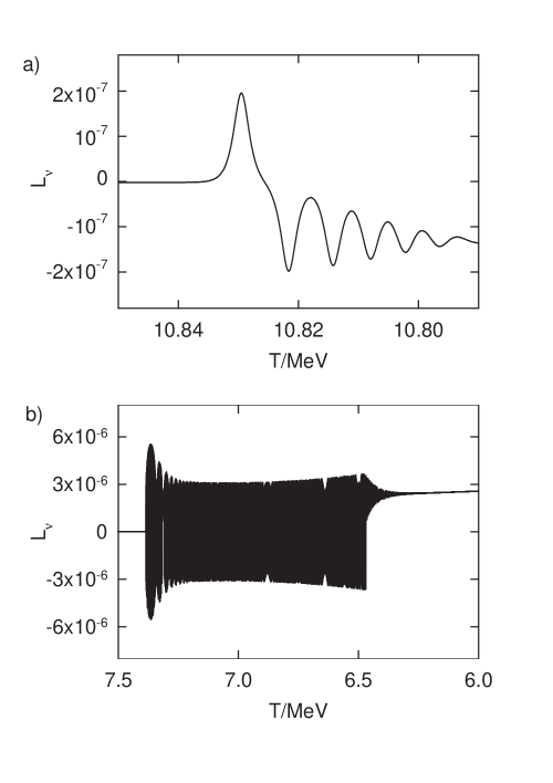
Figure 1: The evolution of the $\nu_{\tau}$-asymmetry in the neigbourhood of the resonance. In Fig. 1a $\delta m^{2}=-10^{-1}$ and $\sin^{2}2\theta=2\times 10^{-9}$; in Fig. 1b $\delta m^{2}=-10^{-2}$ and $\sin^{2}2\theta=2\times 10^{-5}$.

In Fig. 1 we show the asymmetry $L_{\nu_{\tau}}$ (7) resulting from solving equations (9) for two sets of parameters. In Fig. 1a the resonance is rather narrow and only one oscillation occurs before the system is trapped into the minimum with a negative sign of $L_{\nu_{\tau}}$. The subsequent oscillations about this new local minimum are quickly washed away by the damping terms. In contrast, Fig. 1b shows an example of oscillation parameters with which the bifurcation into new local minimum is extremely slow and for a long time there is hardly any barrier between the two minima with opposite signs of $L_{\nu_{\tau}}$, and the system oscillates thousands of times before settling down to a minimum with positive $L_{\nu_{\tau}}$. After settling down, the further evolution of the asymmetry follows a power-like behaviour. These results agree well with those of ref. [15].

It is instructive to look a little more carefully into how the system approaches the resonance. Before the resonance the off-diagonal $P^{\pm}$ components are very near zero and ${P_{z}^{-}}$ near the value $L=0$. Just before the resonance the $P^{+}_{x,y}$ components begin to increase, which triggers both the growth of $P^{-}_{x,y}$ components and the decrease of $P_{z}^{+}$. As $V_{0}$ changes the sign at the resonance it creates an instability in the equation for $P_{y}^{-}$, which eventually strongly pushes $P_{y}^{-}$ to negative direction. The simple coupling of $P_{y}^{-}$ to $P_{z}^{-}$ in (9) then drags $P_{z}^{-}$ along leading to a rapid growth of $L_{\nu_{\tau}}$. So far these phenomena have not much affected the evolution of ${P^{+}}$ variables (which have continued to grow). Eventually however, the exponential growth of ${P^{-}}$ terms causes the $V_{L}$ term in the equations for ${P_{x}^{+}}$ and ${P_{y}^{+}}$, insofar neglible, become dominant. Large $V_{L}$ then forces ${P_{x}^{+}}$ and ${P_{y}^{+}}$ to change sign and grow to opposite direction until $V_{L}$ again changes the sign. Additionally, the ensuing oscillatory motion of the $P^{+}_{x,y}$ components induces the oscillation into other variables as well, leading to the exponentially large oscillation pattern observed in $L_{\nu_{\tau}}$.

To find out the extent of chaotic and/or regular behaviour of sign($L$), we have scanned through the parameter space depicted in Fig. 2, which shows the sign of the final asymmetry $L$ with the initial value $L^{\rm in}=10^{-10}$. As can be seen, the structure of sign($L$) is highly complex. In the upper left hand corner, extending downwards to large $\theta$, there is a regular region with no change in the asymmetry. Its existence is relatively easy to understand: this is the region where only the very first oscillation is carried out before the sign of the asymmetry is fixed. Since the direction of the first oscillation is determined by the sign of the initial asymmetry $L^{\rm in}$ (not necessarily the initial $\nu_{\tau}$-asymmetry), the sign of final neutrino asymmetry in this part of the parameter space should indeed be regular and fully determined.

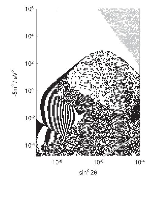
Figure 2: The distribution of the final sign of the neutrino asymmetry in the mixing parameter space. Negative sign($L$) is plotted in black, positive sign($L$) in white. The initial asymmetry was chosen to be $L^{\rm in}=10^{-10}$.

The bands seen in the left hand side of Fig. 2 are formed as the system goes through two or more oscillations. In this region the number of oscillations is slowly increased as $\theta$ grows leading to less determined sign($L$)  but it still can hardly be described as chaotic yet.

In addition to the two more or less regular regions there are regions where sign($L$) appears to be chaotic. The interval $10^{-2}\;\raise 1.29167pt\hbox{$<$\kern-7.5pt\raise-4.73611pt\hbox{$\sim$}}\;|\delta m^{2}|\;\raise 1.29167pt\hbox{$<$\kern-7.5pt\raise-4.73611pt\hbox{$\sim$}}\;1$ contains a very complicated structure. For $|\delta m^{2}|\;\raise 1.29167pt\hbox{$>$\kern-7.5pt\raise-4.73611pt\hbox{$\sim$}}\;1$ one may discern some tendency for positive $L$ to prevail, while the region with $|\delta m^{2}|\;\raise 1.29167pt\hbox{$<$\kern-7.5pt\raise-4.73611pt\hbox{$\sim$}}\;10^{-2}$ appears to be pure white noise. In the lower right-hand corner of Fig. 2 (below the gray line), with $|\delta m^{2}|/\sin^{2}2\theta\;\raise 1.29167pt\hbox{$<$\kern-7.5pt\raise-4.73611pt\hbox{$\sim$}}\;10$, oscillations in $L$ will continue past the neutrino freeze-out and will not settle into any definite value. The boundary of the regular region above which $L$ is positive is given approximately by

$$\left(\log\frac{-\delta m^{2}}{10^{-5.8}\;\mbox{eV}^{2}}\right)^{2}-0.44\left(\log\frac{\sin^{2}2\theta}{10^{4.5}}\right)^{2}\simeq-1.$$ (11)

We conjecture that the chaotic behaviour occurs only when the oscillating period is long. We have also explored in finer detail a restricted region of parameters in the chaotic regime, without finding any structure. It is possible however, that the final sign of $L$ in this region is affected by the accumulated numerical error originating from the extremely high number of oscillation periods. In this sense proving a true chaoticity is of course not possible. Nevertheless, if the system is sensitive to numerical error, it should be expected to be sensitive to parameter fluctuations as well, so the general pattern of rapid sign($L$) fluctuations is expected to be robust. Finally, the region in the upper right-hand corner does not correspond to a large asymmetry, but it is merely the region where $\nu_{s}$ is fully equilibrated [4, 7, 6] and the absolute value of final $L$ is very small.

Changing the initial value for $L^{\rm in}$ does not change the picture qualitatively, although the structures evident in Fig. 2 shift slightly to the left when $L^{\rm in}$ is increased. Moreover, the changes saturate at $L^{\rm in}\;\raise 1.29167pt\hbox{$>$\kern-7.5pt\raise-4.73611pt\hbox{$\sim$}}\;10^{-9}$. These changes, or their absence, are very interesting however: In Fig. 3 we have plotted the value of $L$ at the temperature $T=T_{\rm res}-2.5$, as a function of $L^{\rm in}$ for three representative choices of parameters. The first set, with $\sin^{2}2\theta=10^{-7}$ and $\delta m^{2}=-10^{4}$ eV² corresponds to the stable region with positive $L$ in Fig. 2. As expected, $L$ remains positive independently of the initial value $L^{\rm in}$. In fact the dependence turned out to be smooth and linear showing that not only is the sign robust, but also that the numerical solution is well under control.

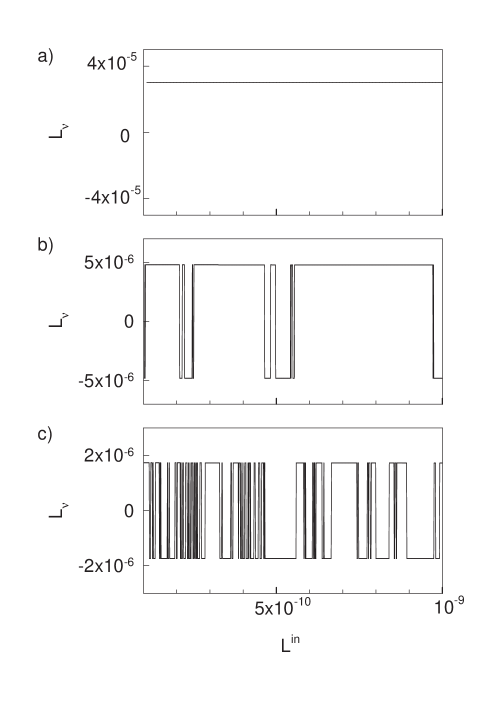
Figure 3: The sign of the asymmetry $L_{\nu_{\tau}}$ at $T=T_{\rm res}-2.5$ MeV as a function of the initial asymmetry $L^{\rm in}$ for three sets of parameters ($\sin^{2}2\theta$, $\delta m^{2}/{\rm eV}^{2}$): a) ($10^{-7}$,$-10^{4}$), b) ($10^{-6}$,$-1$) and c) ($10^{-6}$,$-10^{-3}$).

The second set, with $\sin^{2}2\theta=10^{-6}$ and $\delta m^{2}=-1$ eV², lies in the intermediate region where positive $L$ predominates, and the same dominance is seen as a function of the inital value $L^{\rm in}$. The last set with $\sin^{2}2\theta=10^{-6}$ and $\delta m^{2}=-10^{-3}$ eV² corresponds to the chaotic region. It is evident that sign($L$) is very sensitive to initial conditions, displaying clear randomness as a function of $L^{\rm in}$.

The final value of sign($L$) has consequences for both atmospheric neutrinos and primordial nucleosynthesis. It has been proposed that Super-Kamiokande results for atmospheric neutrinos, which lie in the forbidden zone [4, 6, 7], might still allow a active-sterile mixing solution if the asymmetry growth is taken into account [10]. Although the oscillation parameters in the case of atmospheric neutrinos are in the region where asymmetry growth is not expected, it has been argued that other neutrino oscillations could induce a large asymmetry in the active-sterile sector which the oscillations cannot damp.

If the outcome of neutrino oscillations is highly chaotic, the validity of such a scenario might be suspect. However, we found a large region in the parameter space where sign($L$) is very robust with respect to small variations of the mixing parameters. No chaoticity should be expected there with respect to other small perturbations, such as local perturbations in $L^{\rm in}$, either. It is in these stable domains where one would expect that the mechanism of ref. [10] can be successful.

In the region where sign($L$) is chaotic in the oscillation parameter space, it was also found to be sensitive to fluctuations in $L^{\rm in}$; these are predicted to be generated for example during the QCD phase transition, or in scenarios of electroweak baryogenesis [22, 23, 24]. In such case causally disconnected regions would be expected to develop large asymmetries with a random sign distribution. It has been argued that then the nucleosynthesis constraint on active-sterile mixing would be even more stringent, because of additional MSW conversion taking place in the boundaries of domains with different sign($L$) [25]. However, our results indicate that the new constraints obtained in [25] may be overly optimistic, because for a large part of their excluded region we have found sign($L$) to be stable against small fluctuations; hence in no domain formation should be expected to occur in the first place.

Determining the sign of $L$ is important also for considering the effect of the electron (anti)neutrino spectrum distortions on the light element abundances [16, 21]. When the momentum spectrum gets distorted from its thermal equilibrium value the neutron to proton freezing ratio will change. Direct $\nu_{e}\leftrightarrow\nu_{s}$ oscillations obviously can induce such distortions, but also scenarios where large asymmetry is first generated in $\nu_{\mu,\tau}\leftrightarrow\nu_{s}$ and then transferred to electron neutrino via $\nu_{e}\leftrightarrow\nu_{\mu,\tau}$ oscillation, could have considerable effects on the electron neutrino spectrum. It turns out that positive sign($L$) has the effect of decreasing and negative sign($L$) of increasing ⁴He abundance [16], so that the difference is $\Delta Y\simeq 10^{-2}$, with some dependence on the oscillation parameters. Because the oscillation parameters cannot be measured with an arbitrary accuracy, it follows that in the region where the sign($L$) is chaotic, the role of resonant active-sterile neutrino mixing in Big-Bang Nucleosynthesis can not be reliably estimated. Rather, in this region, depicted in Fig. 2, there always remains an arbitrariness in the ⁴He abundance given by $\Delta Y\simeq 10^{-2}$, which should be considered as a source of systematic error.

In the region where the sign is stable, more concrete conclusions can be drawn. However, in this region $L$ is positive and only a rather small negative shift in the helium abundance $-0.005\;\raise 1.29167pt\hbox{$<$\kern-7.5pt\raise-4.73611pt\hbox{$\sim$}}\;\Delta Y<0$ was found [26] for these parameters. Interestingly enough, such a shift could ameliorate the apparent conflict of the nucleosynthesis theory viz-a-viz observations [14].

Our results in this paper are based on an averaged momentum description of the neutrino ensemble. Some effects, like the diffusion of the asymmetry between different momentum states, would seem to indicate the need for using full momentum-dependent kinetic equations. This is rather hard, since one has to deal with exponential growth in every momentum state and the width of the resonance is, for most of the parameter space, so small that one needs a very large number of bins to complete the task. Our preliminary results with momentum dependent kinetic equations support the results presented here.

This work has been supported by the Academy of Finland under the contract 101-35224.

References

- [1] R. Barbieri and A. Dolgov Phys. Lett. B237 (1990) 440; Nucl. Phys. B237 (1991) 742; K. Kainulainen, Phys. Lett. B244 (191) 1990; K. Enqvist, K. Kainulainen and J. Maalampi, Phys. Lett. B249 (1990) 531; Nucl. Phys. B349 (1991) 754.
- [2] K. Enqvist, K. Kainulainen and J. Maalampi, Phys. Lett. B244 (1990) 186.
- [3] K. Enqvist, K. Kainulainen and M. Thomson, Phys. Lett. B280 (1992) 245.
- [4] K. Enqvist, K. Kainulainen and M. Thomson, Nucl. Phys. B373 (1992) 498.
- [5] J. Cline, Phys. Rev. Lett. 68 (1992) 3137.
- [6] X. Shi, D. Schramm and B. Fields, Phys. Rev. D48 (1993) 2563.
- [7] K. Enqvist, K. Kainulainen and M. Thomson, Phys. Lett. B288 (1992) 145.
- [8] See R. Barbieri and A. Dolgov in ref. [1].
- [9] R. Foot, R.R. Volkas, Phys. Rev. Lett. 75 (1995) 4350.
- [10] R. Foot, M. Thomson and R.R. Volkas, Phys. Rev. D53 (1996) 5349; R. Foot and R.R. Volkas, Phys. Rev. D55 (1997) 5147.
- [11] X. Shi and G.M. Fuller Phys. Rev. D59 (1999) 063006.
- [12] R. Foot and R.R. Volkas, astro-ph/9811067; X. Shi and G.M. Fuller, astro-ph/9812232.
- [13] S. Hannestad and G. Raffelt, Phys. Rev. D59 (1999) 043001.
- [14] K.A. Olive, G. Steigman, T.P. Walker, astro-ph/9905320; S. Burles, K.M. Nollett, J.N. Truran and M.S. Turner, Phys. Rev. Lett. 82 (1999) 4176; K.A. Olive and D. Thomas, Astropart. Phys. 7 (1997) 27.
- [15] X. Shi, Phys. Rev. D54 (1996) 2753.
- [16] R. Foot and R.R. Volkas, Phys. Rev. D56 (1997) 6653, Erratum Phys. Rev. D59 (1999) 029901; X. Shi, G.M. Fuller and K. Abazajian, astro-ph/9905259.
- [17] A. Dolgov, Sov. J. Phys. 33 (1981) 700; B.H.J. McKellar and M.J. Thomson, Phys. Rev. D49 (1994) 2710.
- [18] L. Stodolsky, Phys. Rev. D36 (1987) 2273.
- [19] G. Raffelt, Nucl. Phys. B406 (1993) 423.
- [20] D. Nötzold and G. Raffelt, Nucl. Phys. B307 (1988) 924.
- [21] D.P. Kirilova and M.V. Chizhov, Phys. Lett. B393 (1997) 375; Phys. Rev. D58 (1998) 073004; Nucl. Phys. B534 (1998) 447.
- [22] J.H. Applegate, C.J. Hogan, and R.J. Scherrer, Phys. Rev. 35 (1151) 1987.
- [23] V. Rubakov and M. Shaposhnikov, Usp. Fiz. Nauk 166 (1996) 493; Phys. Usp. 39 (1996) 461; A. Heckler Phys. Rev. D51 (1995) 405; J. Cline, K. Kainulainen and A. Vischer, Phys. Rev. D54 (1996) 2451.
- [24] K. Kainulainen, H. Kurki-Suonio, E. Sihvola, Phys. Rev. D59 (1999) 083505.
- [25] X. Shi and G.M. Fuller, astro-ph/9904041.
- [26] See X. Shi et.al. in ref. [16].