May 1999 SINP/TNP/99-22
Determination of cosmological parameters:
an introduction for non-specialists

Abstract

I start by defining the cosmological parameters $H_{0}$, $\Omega_{m}$ and $\Omega_{\Lambda}$. Then I show how the age of the universe depends on them, followed by the evolution of the scale parameter of the universe for various values of the density parameters. Then I define strategies for measuring them, and show the results for the recent determination of these parameters from measurements on supernovas of type 1a. Implications for particle physics is briefly discussed at the end.

1 Introduction

In this conference on Neutrino Physics, I have been asked to talk about the determination of cosmological parameters. The reason for this, obviously, is the potential importance of neutrinos for cosmology. They can serve as a component for the dark matter of the universe. On the other hand, many important constraints on neutrino properties are derived from various cosmological considerations. The precise values of such constraints are determined by various cosmological parameters like the Hubble parameter, the density of matter in the universe, etc. In the light of this relationship, it is important to know the cosmological parameters accurately. In this talk, I will outline the methods for the determination of cosmological parameters. Since I am not a specialist in this field, at best I can hope that this exposition will be useful to other non-specialists.

The outline of the paper is the following. In Sec. 2, I define the cosmological parameters. There are, in fact, three of them — the Hubble parameter, and the present density of matter energy and vacuum energy in the universe. In Sec. 3, I show how the age of the universe depends on these parameters. Then in Sec. 4, I show how the evolution of the universe depends on the values of the cosmological parameters. An understanding of the evolution is essential in formulating strategies for the cosmological parameters. Some such strategies are discussed in general terms in Sec. 5. At the end of this section, we indicate the outline for the rest of the paper.

2 Defining the cosmological parameters

In cosmology, we start with the the assumption of a homogeneous and isotropic universe, which is described by the Friedman-Robertson-Walker (FRW) metric:

$$ds^{2}=dt^{2}-a^{2}(t)\Bigg{[}{dr^{2}\over 1-kr^{2}}+r^{2}\Big{(}d\theta^{2}+\sin^{2}\theta\,d\phi^{2}\Big{)}\Bigg{]}\,.$$ (2.1)

Here, $r$ is a dimensionless co-ordinate distance and $a(t)$ is an overall scale parameter. The physical distance between two points depends on the co-ordinate distance and the scale parameter, in a manner which will be discussed later. The parameter $k$, if it is non-zero, can always be adjusted to have unit magnitude by adjusting the definition of $r$. Thus, the possible values of $k$ are given by

$$k=0,\pm 1\,.$$ (2.2)

Usually, we think of the universe to be open if $k<0$, for which it expands forever. Contrarily, if $k>0$, the universe is closed, i.e., it is destined to recollapse at some time in the future. The borderline case, $k=0$, is called a flat universe. We will see that these statements are correct only if there is no cosmological constant. From the general consideration of homogeneity and isotropy, however, the cosmological constant can be present, and these notions get modified, as we will see.

In presence of a cosmological constant $\Lambda$, the equations of motion are given by

$$R_{\mu\nu}-\frac{1}{2}g_{\mu\nu}R=8\pi GT_{\mu\nu}+\Lambda g_{\mu\nu}\,.$$ (2.3)

Here, $R_{\mu\nu}$ is the Ricci tensor which is defined through the metric of Eq. (2.1), and $R=R_{\mu\nu}g^{\mu\nu}$. Although in general Eq. (2.3) gives 10 equations, here most of them are identical because the metric is homogeneous and isotropic. In fact, one gets only two independent equations. One of them is given by

$$\left({\dot{a}\over a}\right)^{2}={8\pi G\over 3}\,\rho+{\Lambda\over 3}-{k\over a^{2}}\,,$$ (2.4)

where $\rho$ is the energy density of matter. This equation is valid for all time. Applying it to the present time, we can write

$$H_{0}^{2}={8\pi G\over 3}\,\rho_{0}+{\Lambda\over 3}-{k\over a_{0}^{2}}\,,$$ (2.5)

where $H_{0}$ is the value of $\dot{a}/a$ at the present time, and the subscript ‘0’ on $\rho$ and $a$ denote the values of these parameters at the present time. We now introduce the dimensionless parameters

$$\Omega_{m} \equiv {8\pi G\over 3H_{0}^{2}}\,\rho_{0}\,,$$

$$\Omega_{\Lambda} \equiv {\Lambda\over 3H_{0}^{2}}\,,$$

$$\Omega_{k} \equiv -\;{k\over a_{0}^{2}H_{0}^{2}}\,.$$ (2.6)

These definitions enable us to rewrite Eq. (2.5) in the following form:

$$1=\Omega_{m}+\Omega_{\Lambda}+\Omega_{k}\,.$$ (2.7)

This shows that, among the three parameters introduced in Eq. (2.6), we can take only $\Omega_{m}$ and $\Omega_{\Lambda}$ to be independent. $\Omega_{k}$ is not. In addition, $H_{0}$ is another parameter. These are the three cosmological parameters, and the aim of this lecture is to show how they may be determined.

Before proceeding, I would like to make one comment. Note that all these parameters are defined using values of physical quantities at the present time. One may tend to think that because of that, the present time $t_{0}$ should also be added to the list of parameters. But we will show that in fact $t_{0}$ is not independent.

3 The age of the universe

So far, we have discussed only one of the independent equations that arise among the set given in Eq. (2.3). In order to proceed, we need the other. This is in fact equivalent to the statement of conservation of matter, which means that the quantity $\rho a^{3}$ is constant over time, or

$$\rho a^{3}=\rho_{0}a_{0}^{3}\,.$$ (3.1)

From now on, it is more convenient to use dimensionless variables instead of $a$ and $t$. We define

$$y\equiv{a\over a_{0}}\,,\qquad\tau\equiv H_{0}(t-t_{0})\,.$$ (3.2)

Using these variables, we can rewrite Eq. (2.4) in the following form:

$$\left({dy\over d\tau}\right)^{2} = {y^{2}\over H_{0}^{2}}\left[{8\pi G\over 3}\,{\rho_{0}\over y^{3}}+{\Lambda\over 3}-{k\over y^{2}a_{0}^{2}}\right]$$ (3.3)

$$= {1\over y}\Omega_{m}+y^{2}\Omega_{\Lambda}+\Omega_{k}$$

Eliminating $\Omega_{k}$ now using Eq. (2.7), we obtain

$$\left({dy\over d\tau}\right)^{2}=1+\Big{(}\frac{1}{y}-1\Big{)}\Omega_{m}+\Big{(}y^{2}-1\Big{)}\Omega_{\Lambda}\,,$$ (3.4)

or

$$d\tau={dy\over\sqrt{1+\Big{(}{1\over y}-1\Big{)}\Omega_{m}+\Big{(}y^{2}-1\Big{)}\Omega_{\Lambda}}}\,.$$ (3.5)

If there was a big bang, $y$ was zero at the time of the bang, i.e., at $t=0$. On the other hand, $y=1$ now, by definition. Integrating Eq. (3.5) between these two limits, we obtain

$$H_{0}t_{0} = \int_{0}^{1}{dy\over\sqrt{1+\Big{(}{1\over y}-1\Big{)}\Omega_{m}+\Big{(}y^{2}-1\Big{)}\Omega_{\Lambda}}}\,.$$ (3.6)

This is the equation which shows that the age of the universe is not independent, but rather is determined by $H_{0}$, $\Omega_{m}$ and $\Omega_{\Lambda}$.

Figure 1: Age plots. The lines shown are contours of equal $H_{0}t_{0}$ in the $\Omega_{m}$-$\Omega_{\Lambda}$ plane. Starting from the lower right corner of the plot, the value of $H_{0}t_{0}$ for different lines are $0.5$, $0.6$, $0.7$, $0.8$, $0.9$, $1.0$, $1.2$, $1.5$, $2.0$ and $5.0$. The curve for $H_{0}t_{0}=\infty$ would be virtually indistinguishable from that of $H_{0}t_{0}=5$ in this plot.

Conventionally, one does not use the dimensionless parameter $y$, but rather uses the red-shift parameter $z$, defined by

$$1+z\equiv{a_{0}\over a}={1\over y}\,.$$ (3.7)

Using this variable, Eq. (3.5) becomes

$$d\tau={dz\over 1+z}\;{1\over\sqrt{(1+z)^{2}(1+\Omega_{m}z)-z(2+z)\Omega_{\Lambda}}}\,,$$ (3.8)

so that Eq. (3.6) can be written in the following equivalent form:

$$H_{0}t_{0} = \int_{0}^{\infty}{dz\over 1+z}\;{1\over\sqrt{(1+z)^{2}(1+\Omega_{m}z)-z(2+z)\Omega_{\Lambda}}}\,.$$ (3.9)

In Fig. 1, we have shown contours of equal values of $H_{0}t_{0}$ for different values of $\Omega_{m}$ and $\Omega_{\Lambda}$. For a fixed value of $\Omega_{\Lambda}$, the figure shows that $H_{0}t_{0}$ decreases for increasing values of $\Omega_{m}$. This is because with more matter, the force of gravity is larger, and the initial bang slows down in less time. On the other hand, for fixed $\Omega_{m}$, the age increases with increasing $\Omega_{\Lambda}$. And finally, note that the contour lines for large values of $H_{0}t_{0}$ appear very closer and closer, and approaches asymptotically the line for infinite age. Beyond this line, there is a region in the parameter plane for which the age integral diverges. This is the upper left part of the plot. Later we will discuss what sort of evolution does this part represent.

4 Evolution of the universe

In order to discuss the evolution of the universe, let us not integrate Eq. (3.5) all the way to the initial singularity, but rather to any arbitrary time $t$. This gives

$$H_{0}(t-t_{0})=\int_{0}^{y}{dy^{\prime}\over\sqrt{1+\Big{(}{1\over y^{\prime}}-1\Big{)}\Omega_{m}+\Big{(}y^{\prime 2}-1\Big{)}\Omega_{\Lambda}}}\,.$$ (4.1)

Equivalently, using the red-shift variable, we can write

$$H_{0}(t_{0}-t) = \int_{0}^{z}{dz^{\prime}\over 1+z^{\prime}}\;{1\over\sqrt{(1+z^{\prime})^{2}(1+\Omega_{m}z^{\prime})-z^{\prime}(2+z^{\prime})\Omega_{\Lambda}}}\,.$$ (4.2)

The numerical results of this integration has been shown in Fig. 2 for different values of the pair $(\Omega_{m},\Omega_{\Lambda})$.

Figure 2: Evolution of the scale parameter with respect to time for different values of matter density and cosmological parameter. The horizontal axis represents $H_{0}(t-t_{0})$, the combination which appears in the evolution equation, Eq. (4.1). The vertical axis is $y=a/a_{0}$ in each case. The values of ($\Omega_{m}$,$\Omega_{\Lambda}$) for different plots are: A=(1,0), B=(0.1,0), C=(1.5,0), D=(3,0), E=(0.1,0.9), F=(0,1), G=(3,.1), H=(3,1), I=(.1,.5), J=(.5,$-1$), K=(1.1,2.707), L=(1,2.59), M=(0.1,1.5), N=(0.1,2.5).

Some discussion of these evolution plots are in order. We have shown the plots in six different panels, with some overlaps between them. The first panel represents different examples of universes with $\Omega_{\Lambda}=0$, i.e., no cosmological constant. We know that in this case, the universe closes and collapses to zero volume in the future if $\Omega_{m}>1$. This shows clearly in the curve D, for which $\Omega_{m}=3$. For curve C, the collapsing is not clear in the diagram, but that’s because we have not plotted for large enough values of the time variable. For curve B, $\Omega_{m}=0.1$, and this universe expands forever. Curve A has $\Omega_{m}=1$. Since $\Omega_{\Lambda}=0$, this implies that $\Omega_{k}=0$, i.e., the universe is flat.

In the second panel, we show more flat universes, i.e., universes for which $k=0$, or alternatively $\Omega_{m}+\Omega_{\Lambda}=1$. We see that, subject to this condition, the larger the value of $\Omega_{\Lambda}$, the longer is the past history of the universe. The extreme example is obtained for $\Omega_{\Lambda}=1$, shown as curve F. Although this means $\Omega_{m}=0$ which is unrealistic, since we know there must be some matter in the universe, otherwise who is writing this article and who is going to read it? But in any case, this choice is instructive, and it shows that in this case, the scale parameter started in the infinite past with a zero value, and expanded very slowly for most of the past history of the universe, until recently when it started to grow.

In the third panel, we show universes with $k>0$, i.e., $\Omega_{m}+\Omega_{\Lambda}>1$. One of these curves, viz. D, has been encountered in the first panel already. This one has $\Omega_{m}=3$ and $\Omega_{\Lambda}=0$, and it is destined for a recollapse in the future. If we increases $\Omega_{\Lambda}$ a little bit, viz. to 0.1, we still obtain a recollapsing universe, as shown by the curve G. However, if we take a much larger value of $\Omega_{\Lambda}$, we find a evolution curve like that shown as H. Here, the universe expands forever, despite the fact that $k>0$, or $\Omega_{k}<0$. This is contrary to our intuition obtained from the case of $\Omega_{\Lambda}=0$ universes.

Similar conflict is encountered in the fourth panel, which shows open universes, i.e., universes with $\Omega_{m}+\Omega_{\Lambda}<1$. The curve B, shown earlier in the first panel, shows an evergrowing universe, and so does curve I. But curve J shows a recollapsing universe.

In view of these, let us adopt a more general classification of the different kinds of universes that we have seen. We will keep calling a universe open or closed depending on whether $\Omega_{k}$ is positive or negative. On the other hand, a universe will be called elliptic if it recollapses in the future, and hyperbolic if it is evergrowing. For $\Omega_{\Lambda}=0$, open universes are necessarily hyperbolic and closed universes are elliptic. But for non-zero $\Omega_{\Lambda}$, we can have open hyperbolic, open elliptic, closed hyperbolic or closed elliptic universes.

Before we move on to the next section, we need to discuss the two lower panels of Fig. 2. In the lower left panel, we have repeated curve F which was shown in the second panel of flat universes. As we said, in this case the universe spends an infinite amount of time for which it hardly expands. Curve K gives another example of this kind. For different values of $\Omega_{m}$ and $\Omega_{\Lambda}$, the initial scale parameter is different. These are examples of loitering universes. Curve L shows a universe which is very close to the loitering case. It stays at a particular value of the scale parameter for a long time, but not for infinite amount of time.

If the value of $\Omega_{\Lambda}$ is increased further from those of any of the loitering universe cases in the previous panel, we find bouncing universes, as shown in the last panel. In these cases, the universe started with an infinite scale factor, shrunk to a minimum value at some time in the past and is expanding now. This expansion will go on forever. These are the cases for which the age integral in Eq. (3.6) diverges, and is represented by the empty upper left corner of the age plots of Fig. 1.

Figure 3: Summary of different evolution plots presented in Fig. 2. The borderline between open and closed universes represents flat universes, between hyperbolic and bounce universes represents loitering universes, and the one between elliptic and hyperbolic universes are called critical universes.

All these panels have been summarized in Fig. 3, where we have shown which values of $\Omega_{m}$ and $\Omega_{\Lambda}$ give open or closed universes, as well as hyperbolic or elliptical universes. As we see clearly in this plot, the identification of closed universes with elliptical ones works only for $\Lambda=0$, and so does the identification of open universes with hyperbolic ones.

5 Strategies

We have seen, with many examples, the nature of the evolution of the universe for various values of the cosmological parameters. Now the big question is: how to determine which one is our own universe?

One thing is easy to say, that we do not live in a bouncing universe. The reason is that these universes have a minimum value of $a/a_{0}$, i.e., a certain maximum value for the red-shift parameter $z$, say $z_{\rm max}$. This value satisfies the relation

$$z_{\rm max}^{2}\big{(}z_{\rm max}+3)\leq{2\over\Omega_{m}}\,.$$ (5.1)

We know there exists quasars at $z>4$. So, if we make the reasonable estimate that $\Omega_{m}>0.02$, these cosmologies are ruled out. However, this still leaves us with a vast region in the $\Omega_{m}$-$\Omega_{\Lambda}$ parameter region, and we need to set up a strategy to proceed.

The general (and obvious) strategy is the following. We need to find some observable quantity which depends on the cosmological parameters, determine the value of that observable. That will give us the values for the cosmological parameters. Our original question now shifts to the following one: what is a good observable for this purpose?

We have already encountered one quantity which depends on the cosmological parameters, viz., the age of the universe. Unfortunately, it cannot serve our needs very well. The reason is that one cannot really determine $t_{0}$ from any direct observations. No matter how old an object is found in the universe, that will not determine $t_{0}$, but rather only put a lower limit on it. So we will use estimates of $t_{0}$ only as a check for whatever strategy we adopt.

Another quantity that depends on $\Omega_{m}$ and $\Omega_{\Lambda}$ is the lookback time for any object, which is $t_{0}-t$ that appears in, e.g., Eq. (4.2). We look at a certain object in the sky. We find its red-shift, which can be done very accurately. If we now have some way of knowing the time at which the light that we observe was emitted from the object, we are through. But this cannot be done very well. By looking at the composition of the object and by comparing it with some evolution model, we can probably estimate the age, but it will depend on the evolution model, and so the method is somewhat uncertain.

Therefore one usually relies on the measurement of distances of objects as a function of their redshifts for the purpose of determining cosmological constants. In order to explain the process, first we need to find out how the physical distance of an object depends on $z$ for different values of $\Omega_{m}$ and $\Omega_{\Lambda}$. This issue is taken up in the next section. Following that, in Sec 7, we will discuss some methods of measurements of distances, and summarize how they determine the cosmological constants. The importance of these determinations for particle physics is given in Sec. 8.

6 Distance vs redshift relation

A light ray traces a null geodesic, i.e., a path for which $ds^{2}=0$ in Eq. (2.1). Thus, a light ray coming to us satisfies the equation

$${dr\over dt}={\sqrt{1-kr^{2}}\over a}\,,$$ (6.1)

where $r$ is the dimensionless co-ordinate distance introduced in Eq. (2.1). Using Eqs. (3.7) and (3.8), we can rewrite it as

$${dr\over\sqrt{1+\Omega_{k}a_{0}^{2}H_{0}^{2}r^{2}}}=(1+z){dt\over a_{0}}={1\over H_{0}a_{0}}\;{dz\over\sqrt{(1+z)^{2}(1+\Omega_{m}z)-z(2+z)\Omega_{\Lambda}}}\,,$$ (6.2)

where on the left side, we have replaced $k$ by $\Omega_{k}$ using the definition of Eq. (2.6). Integration of this equation determines the co-ordinate distance as a function of $z$:

$$H_{0}a_{0}r(z)={1\over\sqrt{|\Omega_{k}|}}\;{\rm sinn}\Bigg{[}\sqrt{|\Omega_{k}|}\int_{0}^{z}{dz^{\prime}\over\sqrt{(1+z^{\prime})^{2}(1+\Omega_{m}z^{\prime})-z^{\prime}(2+z^{\prime})\Omega_{\Lambda}}}\Bigg{]}\,,$$ (6.3)

where “sinn” means the hyperbolic sine function if $\Omega_{k}>0$, and the sine function if $\Omega_{k}<0$. If $\Omega_{k}=0$, the sinn and the $\Omega_{k}$’s disappear from the expression and we are left only with the integral.

Figure 4: $H_{0}\ell$ vs. red-shift plots, where $\ell$ is the luminosity distance. From bottom to top, the plots correspond to the choices of $\Omega_{m}$ and $\Omega_{\Lambda}$ denoted by D, A, B, and E in the caption of Fig. 2.

The physical distance to a certain object can be defined in various ways. For what follows, we will need what is called the “luminosity distance” $\ell$, which is defined in a way that the apparent luminosity of any object goes like $1/\ell^{2}$. This is related to the co-ordinate distance [2] by

$$\ell(z)=a_{0}^{2}r(z)/a(z)=(1+z)a_{0}r\,.$$ (6.4)

Thus,

$$H_{0}\ell(z)={1+z\over\sqrt{|\Omega_{k}|}}\;{\rm sinn}\Bigg{[}\sqrt{|\Omega_{k}|}\int_{0}^{z}{dz^{\prime}\over\sqrt{(1+z^{\prime})^{2}(1+\Omega_{m}z^{\prime})-z^{\prime}(2+z^{\prime})\Omega_{\Lambda}}}\Bigg{]}\,.$$ (6.5)

In Fig. 4, we plot $H_{0}\ell(z)$ for various choices of $\Omega_{m}$ and $\Omega_{\Lambda}$ to show the general nature of the variation.

7 Measurement of distances

7.1 General remarks

So let us now ask how one can measure the distance of an object. In a sense, this is the most important problem of observational cosmology. Older methods of measuring distances used ladder techniques [3]. This means that, upto a certain distance, one particular method was used, and this was used to calibrate another method which could be used for larger distances. This process was carried on to higher and higher rungs of the ladder. In order to get to distances large enough to distinguish between different universes, one had to go through several rungs of the ladder, and accordingly there were too many uncertainties in the measurement.

Recently various other methods have been developed and employed to measure the cosmological parameters. These methods avoid using the ladder technique and are therefore expected to provide much better estimates of distances. Some of these are listed below.

Gravitational lensing. Different images of an object from a gravitational lens are formed by light rays coming through different directions, and therefore traversing different path lengths. If the original object has some periodicity in the luminosity, the periodicity of the images will depend on the path length. This provides a way of determining distances [4]. So far, data is very scarce.

Sunayev-Zeldovich effect. Photons from the cosmic microwave background, when passing through a galaxy, get scattered. As a result, they gain in energy. Thus, looking at the direction of a galaxy, the microwave background radiation does not look thermal. Rather, there is some depletion of the low energy photons and some gain of the high energy ones. The amount of this depletion depends on the size of the galaxy. Using this, one can measure the actual sizes of the galaxies. The apparent size observed would then provide a measure for the distance [5]. The data obtained until now show a lot of scatter, and we will not discuss them here.

Microwave background anisotropies. The evolution of density perturbations depend on the values of the cosmological parameters. Therefore, the anisotropies in the microwave background radiation should be predictable in terms of the values of $\Omega_{m}$ and $\Omega_{\Lambda}$. With very accurate determinations of these anisotropies in the near future, this method will probably turn out to be the best probe for the cosmological parameters.

Supernova 1a. In this method, it is assumed that any supernova of type 1a has the same absolute luminosity. The measurement of the apparent luminosity therefore provides a measure for the distance. This will be discussed in more detail in the remaining part.

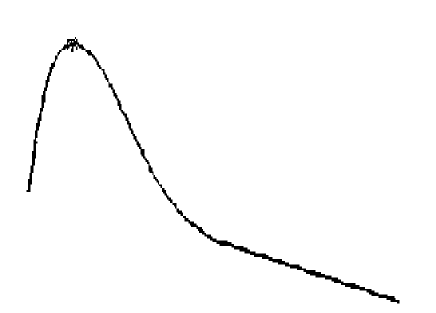
Figure 5: Schematic lightcurve for a supernova of type 1a.

7.2 Results from Supernova 1a measurements

Supernova of type 1a are identified by the nature of their light curve, i.e., the variation of their intensity with time, as shown in Fig. 5. In addition, the spectral analysis reveals lines for heavy elements like magnesium and silicon.

Supernovas of this type are believed to occur due of the merger of two white dwarf stars whose masses are very close to the Chandrasekhar limit. Since the masses entering into the explosion is roughly the same for any supernova 1a, it is reasonable to assume that the intrinsic (or absolute) luminosity of any supernova of this type is the same. Thus, if one measures the apparent luminosity at the maximum of the light curve, this should scale as the inverse square of the distance of the supernova, where the distance is defined to be the luminosity distance. Astronomers use ‘magnitudes’ to denote luminosities, which is a logarithmic representation. Thus, the apparent magnitude at the maximum should satisfy the relation

$$m_{\rm max}\propto\log\ell^{2}\,.$$ (7.1)

We have already shown in Fig. 4 how $\log\ell$ varies with $z$ for different values of $\Omega_{m}$ and $\Omega_{\Lambda}$. So the strategy must be simple. One should plot the observed values of the distance vs $z$, and determine which pairs of values of $\Omega_{m}$ and $\Omega_{\Lambda}$ give the best fit for the observed points.

There is only one small point to settle before embarking on this program. The vertical axis of Fig. 4 gives the logarithmic values of $H_{0}\ell$, not of $\ell$. Thus, unless we know what $H_{0}$ is, we cannot proceed. However, the thing to note is that for small values of $z$, the plots are independent of $\Omega_{m}$ and $\Omega_{\Lambda}$. Thus, if one determines the red-shifts and apparent magnitudes of nearby supernovas, that should determine the Hubble parameter. Using this value then, one can go over to larger values of $z$ and determine $\Omega_{m}$ and $\Omega_{\Lambda}$.

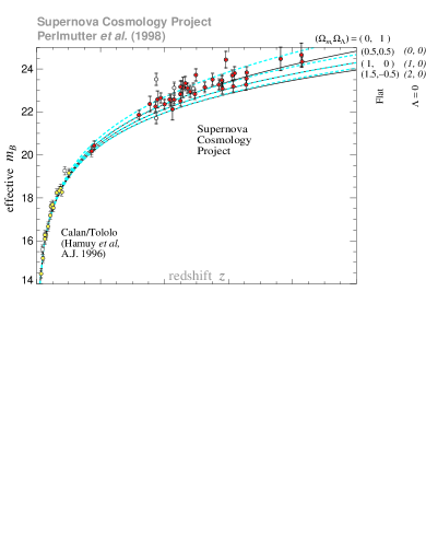
Figure 6: Results of redshift vs. apparent luminosity of a number of type-1 supernovas. The horizontal scale goes from 0 to 1. The data for low redshift are from Ref. [6], and for $z>0.2$ is from Ref. [7]. The figure is taken from Ref. [7], with slight modification of the legends. The dashed lines are for flat universes, and the solid lines for $\Lambda=0$ universes, with values of $\Omega_{m}$ and $\Omega_{\Lambda}$ given at the top right corner.

The part of the task at low $z$ was extensively done a few years ago [6], and the data are shown in Fig. 6. The value of the Hubble parameter obtained from this data is:

$$H_{0}=(63.1\pm 3.4\pm 2.9)\ \rm km\,s^{-1}\,Mpc^{-1}\,.$$ (7.2)

Using this value, one can determine the distances of farther supernovas. This has been started in 1998 under the team effort called the ‘Supernova Cosmology Project’ (SCP). They measured the redshift and the effective magnitude of 42 supernovas and published their result, which is shown in Fig. 6. Superimposed on their data are the results expected from different combinations of $\Omega_{m}$ and $\Omega_{\Lambda}$. Apart from an overall normalization, these are the curves as shown in Fig. 4. One can now determine which values of $\Omega_{m}$ and $\Omega_{\Lambda}$ fit the data sufficiently well, and the results of the analysis of the SCP has been shown in Fig.7.

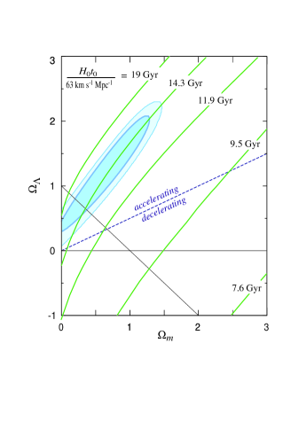
Figure 7: Best fits for the data of Fig. 6 in the $\Omega_{m}$-$\Omega_{\Lambda}$ plane. Superimposed are the contours of equal age, with the value of the Hubble parameter set at $63\ \rm km\,s^{-1}\,Mpc^{-1}$.

Clearly, the fits show that the cosmological constant is non-zero. In fact, if we stick to flat universes, which are denoted by the diagonal straight line on this plot, the best value that the SCP advocate is

$$\Omega_{m}\approx 0.22\,,\qquad\Omega_{\Lambda}\approx 0.78\,.$$ (7.3)

In general, however, we obtain a region in the plane, and the regions allowed at different confidence levels are shown on the plot.

In Fig. 1, we have seen how these contours look like. In general, one obtains contours of equal $H_{0}t_{0}$. Assuming a value of $H_{0}$, one can draw contours of equal age, which have also been superposed on the plot of Fig. 7. The value of $H_{0}$ assumed is inspired by the results shown in Eq. (7.2), and is indicated in the figure and the caption. The best fit that the SCP advocate is:

$$t_{0}=(14.9\pm 1)\times 10^{9}\rm yr\,,$$ (7.4)

for flat universes. If one does not assume a flat universe, the best fit for the age is

$$t_{0}=(14.5\pm 1)\times 10^{9}\rm yr\,.$$ (7.5)

Of course, both these values for $t_{0}$ are for the value of $H_{0}$ indicated in the figure, which is the central value quoted in Eq. (7.2).

8 Implications

What do these result mean for particle physics? Various particles, like neutrinos, can contribute only to $\Omega_{m}$. The central value of the Hubble parameter, taken literally, tells us that the critical density of the universe is

$$\rho_{c}=4\;{\rm keV/cm}^{3}\,.$$ (8.1)

Moreover, taking the best values advocated in Eq. (7.3), we obtain that the matter density in the present universe is

$$\rho_{0}\approx 900\;{\rm eV/cm}^{3}\,.$$ (8.2)

With the standard number density of neutrinos of about 110/cm³, the maximum allowed mass for light stable neutrinos is about 8 eV. One can similarly go through various other constraints on neutrino properties derived from cosmology, and find that they become much more stringent than the values usually quoted.

And this is not all. As we already pointed out, the growth of density perturbations have different characteristics in a universe with non-zero $\Lambda$. These considerations also put extra constraints on different types of possible dark matter. This is a subject which is only beginning to be investigated [8].

References

- [1] S. M. Carroll, W. H. Press, E. L. Turner: Ann. Rev. Astron. Astrophys. 30 (1992) 499.
- [2] A. P. Lightman, W. H. Press, R. H. Price, S. A. Teukolsky: Problem book in relativity and gravitation, (Princeton University Press, 1975).
- [3] For a discussion of these older techniques, see, e.g., G. Bothun: Modern cosmological observations and problems, (Taylor & Francis, 1998).
- [4] For details, see, e.g., R. D. Blandford and R. Narayan: Ann. Rev. Astron. Astrophys. 30 (1992) 311.
- [5] For details, see, e.g., Y. Rephaeli: Ann. Rev. Astron. Astrophys. 33 (1995) 541; M. Birkinshaw: Phys. Rep. 310 (1999) 97.
- [6] M. Hamuy, M. M. Phillips, N. B. Suntzeff, R. A. Schommer, J. Maza, R. Avilés: Astronom. J. 112 (1996) 2391.
- [7] The Supernova Cosmology Project, S. Perlmutter et al, astro-ph/9812133.
- [8] See, e.g., J.R. Primack and M.A. Gross, astro-ph/9810204.