Abstract

We compute in the instanton vacuum the nucleon matrix elements of the twist–4 QCD operators describing power corrections to the second moments of the unpolarized structure functions, $F_{L}$ and $F_{2}$. Our approach takes into account the leading contribution in the packing fraction of the instanton medium, $\bar{\rho}/\bar{R}\ll 1$. Parametrically leading are the matrix elements of a twist–4 quark–gluon operator, which are of the order of the inverse instanton size, $1/\bar{\rho}^{2}=(600\,{\rm MeV})^{2}$. The matrix elements of the four–fermion (diquark) operators are suppressed by a factor $(\bar{\rho}/\bar{R})^{4}$ and numerically small. These results are in agreement with the pattern of phenomenological $1/Q^{2}$–corrections to $R=\sigma_{L}/\sigma_{T}$ and $F_{2}$ found in QCD fits to the data. In particular, the rise of $R$ at low $Q^{2}$ can be obtained from instanton–type vacuum fluctuations at a low scale.

PACS: 13.60.Hb, 12.38.Lg, 11.15.Kc, 12.39.Ki
Keywords: unpolarized structure functions, higher–twist effects, instantons, $1/N_{c}$–expansion  
¹ E-mail: birgitd@tp2.ruhr-uni-bochum.de
² E-mail: maul@nordita.dk
³ E-mail: weiss@tp2.ruhr-uni-bochum.de

1 Introduction

An outstanding problem in the theory of deep–inelastic scattering is to understand the transition from the asymptotic region, where the scale dependence of structure functions is described by perturbative evolution, to the region of low $Q^{2}$, where non-perturbative effects play an essential role. Starting from high $Q^{2}$, the onset of non-perturbative effects manifests itself in power ($1/Q^{2}$–) corrections, which are governed by non-perturbative scale parameters. Aside from the well–understood target mass corrections there are dynamical power corrections, which in QCD are determined by nucleon matrix elements of operators of non–leading twist $(>2)$ [1, 2, 3]. In the partonic language, they describe the effects of the interaction of the quarks with the non-perturbative gluon field in the nucleon, or of 2–body correlations between quarks, on the DIS cross section. A well–known example are the longitudinal structure function $F_{L}=F_{2}-2xF_{1}$, or the ratio $R=\sigma_{L}/\sigma_{T}$, which both happen to be zero in the naive parton model (i.e., without radiative corrections). QCD fits of the data, using existing NLO parametrizations to describe the twist–2 contribution, leave room for sizable $1/Q^{2}$–power corrections [4, 5, 6, 7]. It remains a challenge to understand the origin of these corrections from first principles.

During the last years there has been mounting evidence for an important role of instanton–type vacuum fluctuations in determining the properties of the low–energy hadronic world [8]. The so-called instanton vacuum is a variational approximation to the ground state of Yang–Mills theory in terms of a “medium” of instantons and antiinstantons, with quantum fluctuations about them, which is stabilized by instanton interactions [9]. The strong coupling constant is fixed at a scale of the order of the inverse average size of the instantons in the medium, $\bar{\rho}^{-1}\simeq 600\,{\rm MeV}$. The most important property of this picture, which had been postulated on phenomenological grounds by Shuryak [10] and was later established in the variational calculation of Diakonov and Petrov [9], is the diluteness of the instanton medium, i.e., the fact that the ratio of the average size of instantons in the medium to their average distance, $\bar{R}$, is small: $\bar{\rho}/\bar{R}\simeq 1/3$. The existence of this small parameter makes possible a systematic analysis of non-perturbative effects in this approach.

In particular, the instanton vacuum explains the dynamical breaking of chiral symmetry, which is crucial in determining the structure of strong interactions at low energies [11, 12]. It happens due to the delocalization of the fermionic zero modes associated with the individual (anti–) instantons in the medium. Using the $1/N_{c}$–expansion one derives from the instanton vacuum an effective low–energy theory, whose degrees of freedom are pions (Goldstone bosons) and massive “constituent” quarks. The nucleon is described as a chiral soliton in this effective theory, as a state of $N_{c}$ “valence” quarks bound by a classical pion field [13].

The instanton vacuum has also received strong support from direct lattice simulations. Not only were the basic characteristics of the instanton medium reproduced after “cooling” of the quantum fluctuations [14], also the correlation functions of various hadronic currents were found to remain practically unchanged under cooling, showing that the instanton vacuum takes into account the relevant non-perturbative fluctuations in these channels.

Given the general success of the instanton vacuum in describing hadronic properties, it is natural to ask if this scheme of approximations can explain the non-perturbative effects observed in the scale dependence of structure functions at low $Q^{2}$. More ambitiously, one could also ask the opposite question: Can we use the rich and increasingly accurate information obtained from DIS to learn something about properties of non-perturbative vacuum fluctuations?

The aim of this paper is to study the $1/Q^{2}$–power corrections to unpolarized structure functions, in particular, to the longitudinal structure function, $F_{L}$, in the instanton vacuum. We restrict ourselves to the lowest moments, for which the power corrections can be studied using the operator product expansion (OPE) [1, 2]. In particular, we use the instanton vacuum to compute the nucleon matrix elements of the twist–4 operators, both the quark–gluon and the four–quark operators, and discuss their relative magnitude. Our approach takes into account the leading contribution in the packing fraction of the instanton medium, $\bar{\rho}/\bar{R}$ [15, 16]. Our main conclusion is that the matrix element of the twist–4 quark–gluon correlator is parametrically large and accounts for most of the observed scaling violations in $F_{L}$, while the four–fermionic operators are suppressed.

The quantitative description of power corrections is a complex problem. The set of higher–twist operators used in the OPE is over complete, since matrix elements of different operators are related by the QCD equations of motion. In order to have results which are independent of the choice of the operator basis one needs to make consistent approximations in dealing with the QCD operators and with the nucleon state, something which is generally impossible to achieve in phenomenological approaches such as the bag model [2]. In this respect the instanton vacuum with its inherent small parameter, $\bar{\rho}/\bar{R}$, offers some decisive methodological advantages. As was shown in Ref.[16], in this approach the QCD equations of motion are preserved at the level of effective operators, which is a consequence of the one–instanton approximation justified in leading order of $\bar{\rho}/\bar{R}$, and of the fact that the fermions couple to the instanton through the zero mode, see [16] for details. It is crucial in this context that the description of the nucleon as a chiral soliton is a fully field–theoretic one and does not involve any additional dynamical input besides the chiral symmetry breaking induced by the instanton fluctuations. Also, it should be pointed out that, contrary to other field–theoretic approaches such as QCD sum rules or lattice calculations our approach is based on a small parameter, $\bar{\rho}/\bar{R}$, which endows the a priori structure-less set of higher–twist matrix elements with a parametric order, thus greatly simplifying the discussion of power corrections.

The plan of this paper is as follows. In Section 2, we summarize the QCD predictions for the scale dependence of the unpolarized structure functions $F_{L}$ and $F_{2}$ to order $1/Q^{2}$, including twist–2, target mass and dynamical twist–4 corrections. The central part of the paper, Section 3, is devoted to the calculation of the relevant twist–4 matrix elements in the instanton vacuum. Subsection 3.1 describes the basic properties of the instanton vacuum and the resulting low-energy effective chiral theory. In Subsection 3.2 we outline the method by which the QCD twist–4 operators can be mapped onto effective operators, whose matrix elements can be computed in the low-energy effective theory [16]. As a novel feature, we show here that the QCD twist–4 quark–gluon operators which produce parametrically large matrix elements in $\bar{\rho}/\bar{R}$ can be represented in the effective theory by one–body operators built from the massive “constituent” quark field. This representation turns out to be very convenient both for discussing general properties of instanton–induced higher–twist effects, as well as for computing the nucleon matrix elements. In Subsection 3.3 we compute the nucleon matrix elements of the effective operators, within the large–$N_{c}$ picture of the nucleon as a chiral soliton. In Section 4 we use the instanton results for the twist–4 matrix elements to estimate the scale dependence of $F_{L}$ and $F_{2}$, and compare with the data for $R=\sigma_{L}/\sigma_{T}$ and $F_{2}$. We also compare our results for the matrix elements with those of other theoretical approaches. Conclusions and an outlook are presented in Section 5.

Appendix A contains a short derivation of the QCD expressions for the dynamical twist–4 corrections to unpolarized structure functions using the operator product expansion [1]. Since calculations of higher–twist effects are highly dependent on conventions we explicitly state all relevant conventions there.

We are not considering here power corrections to DIS structure functions resulting from instanton contributions to the coefficient functions of the OPE, i.e., semiclassical corrections associated with single instantons of size $\rho\sim 1/Q$ [17, 18]. These are suppressed by very large powers of $1/Q$ and typically negligibly small. Rather, we use a medium of instantons of average size $\bar{\rho}=(600\,{\rm MeV})^{-1}$ as a model for the non-perturbative vacuum structure at the hadronic scale, in order to calculate the matrix elements parametrizing $1/Q^{2}$–corrections.

The power corrections to $F_{L}$ and $R=\sigma_{L}/\sigma_{T}$ have been estimated previously in a variety of models. In the so-called transverse basis of twist–4 operators the $1/Q^{2}$–corrections to $F_{L}$ can be related to an “intrinsic” transverse momentum of the partons [3]. This language is frequently used to model dynamical twist–4 contributions. A model interpolating between large $Q^{2}$ and the limit $Q^{2}\rightarrow 0$ has been proposed in Ref.[19]. In Ref.[20] the leading–order twist–4 contribution at large $x$ has been related to the derivative of the twist–2 distribution. Also, the magnitude of the twist–4 contribution to $F_{L}$ has been estimated from the renormalon ambiguity of the perturbation series for the $O(\alpha_{S})$ twist–2 coefficient functions calculated in the large–$N_{f}$ limit [21, 22]. In Ref.[23] an attempt was made to model the non-perturbative twist–4 contribution at large $x$ by introducing a coupling to vacuum condensates. Higher–twist contributions to unpolarized structure functions have also been studied in the bag model [24, 25].

2 Power corrections to unpolarized DIS

The hadronic tensor for unpolarized electromagnetic scattering off the nucleon has two independent symmetric structures, which are parameterized in terms of the two structure functions $F_{1}$ and $F_{2}$, or, equivalently, $F_{L}\equiv F_{2}-2xF_{1}$ and $F_{2}$:

$$W_{\mu\nu}(p,q) \equiv \frac{1}{4\pi}\int d^{4}z\;e^{iq\cdot z}\langle p|\,\,J_{\mu}^{\dagger}(z)\,J_{\nu}(0)\,\,|p\rangle$$ (2.1)

$$= \frac{F_{L}(x,Q^{2})}{2x}\left(g_{\mu\nu}-\frac{q_{\mu}q_{\nu}}{q^{2}}\right)$$

$$+ \;\frac{F_{2}(x,Q^{2})}{2x}\left[\frac{-q^{2}}{(p\cdot q)^{2}}p_{\mu}p_{\nu}+\frac{1}{p\cdot q}(p_{\mu}q_{\nu}+p_{\nu}q_{\mu})-g_{\mu\nu}\right].$$

Here, $J_{\mu}(z)=J_{\mu}^{\dagger}(z)$ is the electromagnetic current operator, $p_{\mu}$ the nucleon momentum ($p^{2}=M_{N}^{2}$), $x\equiv-q^{2}/(2p\cdot q)$ and $Q^{2}\equiv-q^{2}$. Here and in the following, all matrix elements are understood to be averaged over the target spin,

$$\langle p|\ldots|p\rangle \equiv {\textstyle{\frac{1}{2}}}\sum_{S}\langle pS|\ldots|pS\rangle,$$ (2.2)

and the states are normalized according to $\langle p^{\prime}|p\rangle=2p^{0}(2\pi)^{3}\delta^{(3)}({\bf p}^{\prime}-{\bf p})$. In connection with experiments one frequently uses a slightly modified definition of the longitudinal structure function [5]:

$$\widetilde{F}_{L}(x,Q^{2}) \equiv F_{2}(x,Q^{2})\left(1+\frac{4M_{N}^{2}x^{2}}{Q^{2}}\right)-2xF_{1}(x,Q^{2})$$ (2.3)

$$= F_{L}(x,Q^{2})+\frac{4M_{N}^{2}x^{2}}{Q^{2}}F_{2}(x,Q^{2}).$$

This function is directly related to the experimentally measured ratio $R=\sigma_{L}/\sigma_{T}$, namely

$$\widetilde{F}_{L}(x,Q^{2}) = F_{2}(x,Q^{2})\left(1+\frac{4M_{N}^{2}x^{2}}{Q^{2}}\right)\frac{R(x,Q^{2})}{R(x,Q^{2})+1}.$$ (2.4)

In QCD, the electromagnetic current is carried by the quark field,

$$J_{\mu}(z) = \sum_{f}e_{f}\bar{\psi}_{f}(z)\gamma_{\mu}\psi_{f}(z),$$ (2.5)

where $e_{f}$ are the quark charges. The scale dependence of the moments of the structure functions up to level $1/Q^{2}$ can be determined by relating the hadronic tensor to the imaginary part of the forward amplitude for the scattering of a virtual photon off the nucleon, and applying the operator product expansion (OPE) to the time–ordered product of electromagnetic currents in the latter [1, 2]. A short summary of this approach, including all relevant conventions, is given in Appendix A. We consider here the second moments of the structure functions:

$$\left.\begin{array}[]{r}\widetilde{M}_{L}(2,Q^{2})\\[4.30554pt] M_{2}(2,Q^{2})\end{array}\right\} \equiv \int_{0}^{1}dx\;\left\{\begin{array}[]{r}\widetilde{F}_{L}(x,Q^{2})\\[4.30554pt] F_{2}(x,Q^{2})\end{array}\right..$$ (2.10)

We distinguish between the scaling (non–power suppressed) part of these moments, which comes from the contribution of twist–2 spin–2 operators in the OPE, the target mass corrections ($\propto M_{N}^{2}/Q^{2}$), which arise from twist–2 spin–4 operators, and the dynamical power corrections coming from contributions of operators of twist 4 and spin 2.

In the case of the longitudinal structure function the twist–2 contribution is of order $\alpha_{S}$, since $F_{L}$ is zero in the naive parton model due to the Callan–Gross relation. The coefficient functions have been computed in Ref.[5], see also Refs.[22, 26]. In leading order:

$$\widetilde{M}_{L}(2,Q^{2})^{\rm twist-2} = \frac{\alpha_{S}(Q^{2})}{4\pi}\left[\frac{4C_{F}}{3}\sum_{f}e_{f}^{2}L^{(2)}_{f}\;+\;\frac{2}{3}\left(\sum_{f}e_{f}^{2}\right)L^{(2)}_{G}\right],$$ (2.11)

$$M_{2}(2,Q^{2})^{\rm twist-2} = \sum_{f}e_{f}^{2}L^{(2)}_{f}$$ (2.12)

$$+ \frac{\alpha_{S}(Q^{2})}{4\pi}\left[\frac{C_{F}}{3}\sum_{f}e_{f}^{2}L^{(2)}_{f}\;-\;\frac{1}{2}\left(\sum_{f}e_{f}^{2}\right)L^{(2)}_{G}\right],$$

where $C_{F}=4/3$ and the sums run over all light flavors ($u,d$ and $s$) in the target. Here $L^{(n)}_{f},L^{(n)}_{G}$ denote the matrix elements of the twist–2 spin–$n$ quark and gluon operators in the target,

$$\left.\begin{array}[]{rcr}\langle p|\;\bar{\psi}_{f}\gamma_{\mu_{1}}i\nabla_{\mu_{2}}\ldots i\nabla_{\mu_{n}}\psi_{f}\;|p\rangle-\mbox{traces}&=&2L^{(n)}_{f}\\[8.61108pt] \langle p|\;F_{\mu_{1}\alpha}D_{\mu_{2}}\ldots D_{\mu_{n-1}}F^{\alpha}_{\;\;\mu_{n}}\;|p\rangle-\mbox{traces}&=&2L^{(n)}_{G}\end{array}\right\}\times\left(p_{\mu_{1}}\ldots p_{\mu_{n}}-\mbox{traces}\right),$$ (2.15)

where on the L.H.S. complete symmetrization in $\mu_{1}\ldots\mu_{n}$ is implied. Here

$$\nabla_{\mu} \equiv \partial_{\mu}-iA_{\mu}^{a}(x)\frac{\lambda^{a}}{2},$$ (2.16)

with ${\rm tr}[\lambda^{a}\lambda^{b}]=2\delta^{ab}$, is the covariant derivative in the fundamental representation of $SU(3)$,

$$F_{\mu\nu} \equiv i\left[\nabla_{\mu},\nabla_{\nu}\right]\;\;=\;\;F_{\mu\nu}^{a}\frac{\lambda^{a}}{2}$$ (2.17)

the gauge field, and

$$(D_{\alpha}F_{\mu\nu})^{a} = \partial_{\alpha}F_{\mu\nu}^{a}-f^{abc}A_{\alpha}^{b}F_{\mu\nu}^{c}$$ (2.18)

the covariant derivative in the adjoint representation.

The target mass corrections to the second moments are proportional to the matrix element of the spin–4 twist–2 operator (see Refs.[1, 3] and Appendix A):

$$\widetilde{M}_{L}(2,Q^{2})^{\rm target\;mass} = \frac{M_{N}^{2}}{Q^{2}}\sum_{f}e_{f}^{2}L^{(4)}_{f},$$ (2.19)

$$M_{2}(2,Q^{2})^{\rm target\;mass} = \;\;\frac{M_{N}^{2}}{2Q^{2}}\sum_{f}e_{f}^{2}L^{(4)}_{f},$$ (2.20)

where we have restricted ourselves to the $O(\alpha_{S}^{0})$ (tree–level) coefficient function.

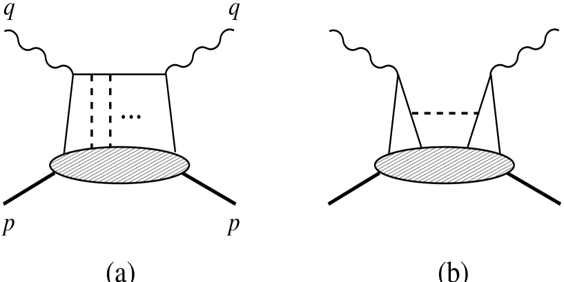
Figure 1: The two types of twist–4 contributions to the DIS cross section. (a) Interference between scattering of the photon off a free quark and scattering off a quark interacting with the non-perturbative gluon field of the nucleon. (b) Interference between scattering off two different quarks in the nucleon, with a perturbative gluon exchange.

Our main object of interest are the dynamical power corrections, which are determined by matrix elements of twist–4 spin–2 operators [1, 2]. There are two types of twist–4 contributions, shown schematically in Fig.1, resulting from different contractions of the quark fields in the two electromagnetic current operators. Contribution (a) describes the interference of the scattering of the photon off a free quark with scattering off a quark interacting with the non-perturbative gluon field in the target; this contribution gives rise to matrix elements of twist–4 quark–gluon operators in the target. Contribution (b) describes the interference of scattering off two different quarks in the target, accompanied by a perturbative gluon exchange; it leads to matrix elements of four–fermionic (“diquark”) operators in the target. In the longitudinal structure function the latter contribution is absent. We have recalculated the coefficient functions of the twist–4 operators, following the approach of Ref.[1], and reproduced the results given in that paper. A short outline of the calculation is given in Appendix A. For the second moment of the longitudinal structure function one finds

$$\widetilde{M}_{L}(2,Q^{2})^{\rm twist-4} = \frac{1}{Q^{2}}\sum_{f}e_{f}^{2}\left(-\frac{1}{4}A_{f}+\frac{3}{4}B_{f}\right).$$ (2.21)

Again we have restricted ourselves to the tree–level coefficient function. Here, $A_{f}$ and $B_{f}$ [their dimension is $(\mbox{mass})^{2}$] denote the reduced matrix elements of the twist–4 spin–2 operators:

$$A_{\alpha\beta,\;f} = \bar{\psi}_{f}\gamma_{\alpha}(D^{\gamma}F_{\gamma\beta})\psi_{f}\;-\;\mbox{trace},$$ (2.22)

$$B_{\alpha\beta,\;f} = \bar{\psi}_{f}\gamma^{\gamma}\gamma_{5}i\left(\nabla_{\alpha}\widetilde{F}_{\beta\gamma}+\widetilde{F}_{\alpha\gamma}\nabla_{\beta}\right)\psi_{f}\;-\;\mbox{trace},$$ (2.23)

with

$$\langle p|\left\{\begin{array}[]{r}A_{\alpha\beta,\;f}\\[4.30554pt] B_{\alpha\beta,\;f}\end{array}\right\}|p\rangle = 2\left\{\begin{array}[]{r}A_{f}\\[4.30554pt] B_{f}\end{array}\right\}\times\left(p_{\alpha}p_{\beta}-{\textstyle{\frac{1}{4}}}p^{2}g_{\alpha\beta}\right).$$ (2.28)

It is understood that the operators are symmetrized in the Lorentz indices according to $A_{\alpha\beta}\rightarrow\frac{1}{2}(A_{\alpha\beta}+A_{\beta\alpha})$; this will not be explicitly indicated in the following. Here

$$\widetilde{F}^{\mu\nu} = \frac{1}{2}\epsilon^{\mu\nu\rho\sigma}F_{\rho\sigma}$$ (2.29)

is the dual field strength. We are using the convention $\gamma_{5}=-i\gamma^{0}\gamma^{1}\gamma^{2}\gamma^{3}$ (as in Refs.[1, 11, 15, 16]), which differs from the one of Bjorken and Drell by a minus sign, and $\epsilon^{0123}=1$. Note that, using the QCD equations of motion, one can replace the forward matrix element of the operator $A_{\alpha\beta,\;f}$ by that of a four–fermionic operator:

$$A_{\alpha\beta,\;f} \rightarrow -g^{2}\left(\bar{\psi}_{f}\frac{\lambda^{a}}{2}\gamma_{\alpha}\psi_{f}\right)\left(\sum_{f^{\prime}}\bar{\psi}_{f^{\prime}}\frac{\lambda^{a}}{2}\gamma_{\beta}\psi_{f^{\prime}}\right).$$ (2.30)

In the case of the structure function $F_{2}$ one has to consider also the twist–4 contributions of type Fig.1 (b), which can be computed using standard Feynman rules. One finds

$$M_{2}(2,Q^{2})^{\rm twist-4} = \frac{1}{Q^{2}}\sum_{f}e_{f}^{2}\left(-\frac{5}{8}A_{f}-\frac{1}{8}B_{f}\right)+\frac{1}{Q^{2}}\sum_{f,f^{\prime}}e_{f}e_{f^{\prime}}C_{ff^{\prime}}\;,$$ (2.31)

where $C_{ff^{\prime}}$ denotes the reduced matrix element [cf. Eq.(2.28)] of the four–fermionic operator

$$C_{\alpha\beta,\;ff^{\prime}} = g^{2}\left(\bar{\psi}_{f}\frac{\lambda^{a}}{2}\gamma_{\alpha}\gamma_{5}\psi_{f}\right)\left(\bar{\psi}_{f^{\prime}}\frac{\lambda^{a}}{2}\gamma_{\beta}\gamma_{5}\psi_{f^{\prime}}\right).$$ (2.32)

3 Twist–4 contribution to $F_{L}$ and $F_{2}$ from instantons

3.1 Instanton vacuum and low–energy effective theory

The framework for our calculation of matrix elements of QCD operators is the instanton–based vacuum of Diakonov and Petrov [9], which is a variational estimate of the Euclidean Yang–Mills (“quenched QCD”) partition function in terms of configurations consisting of a superposition of instantons and antiinstantons ($I$’s and $\bar{I}$’s), with quantum fluctuations about them. The medium of $I$’s and $\bar{I}$’s stabilizes due to an effective repulsion between the pseudoparticles. The resulting statistical ensemble turns out to be well described by a partition function of independent $I$’s and $\bar{I}$’s with an effective size distribution, with average size $\bar{\rho}=(600\,{\rm MeV})^{-1}$. In the large–$N_{c}$ limit the size distribution is sharply peaked, so one may take the sizes of all $I$’s and $\bar{I}$’s to be equal to $\bar{\rho}$. An important property, which is in fact crucial for this picture to be consistent, is the diluteness of the medium of $I$’s and $\bar{I}$’s. In the approach of Ref.[9] the ratio of the average size of instantons to their average distance in the medium was found to be $\bar{\rho}/\bar{R}\simeq 1/3\ll 1$. This fact can be traced back to the “accidentally” large value of the coefficient of the one–loop beta function of QCD, $b\equiv 11N_{c}/3\approx 10$.

When quarks are included, the dynamical breaking of chiral symmetry is a consequence of the interaction of the quarks with the fermionic zero modes associated with the individual instantons [11]. The most compact way to express this is through an effective low–energy theory, which has been derived in the large–$N_{c}$ limit using the so-called zero mode approximation (which is exact in leading order of $\bar{\rho}/\bar{R}$) [12, 15]. It can be formulated in terms of quark fields ($N_{f}$ flavors) with a dynamical mass and a Goldstone bosons (pion) field, with an effective action

$$S_{\rm eff} = \int d^{4}x\sum_{f,f^{\prime}=1}^{N_{f}}\psi^{\dagger}_{f^{\prime}}(x)\left[\delta_{f^{\prime}f}\;(-i)\gamma_{\mu}\partial_{\mu}\;-\;iMF(-\!\stackrel{{\scriptstyle\leftarrow}}{{{}\partial^{2}}})\,U^{\gamma_{5}}(x)_{f^{\prime}f}\,F(-\!\stackrel{{\scriptstyle\rightarrow}}{{{}\partial^{2}}})\right]\psi_{f}(x).\;\;\;\;\;\;\;$$ (3.1)

We have passed to Euclidean field theory by continuing the time dependence of the fields to imaginary times and introducing Euclidean fields and gamma matrices according to the conventions given in Appendix B. (Unless stated otherwise, all formulas in Subsections 3.1 and 3.2 will be written in terms of Euclidean quantities.) In Eq.(3.1), $M$ is the dynamical quark mass; parametrically it is of order

$$M\bar{\rho} \sim \left(\frac{\bar{\rho}}{\bar{R}}\right)^{2}.$$ (3.2)

The pion field, $\pi(x)$, couples to the quarks in a chirally invariant way,

$$U^{\gamma_{5}}(x) = \frac{1+\gamma_{5}}{2}U(x)+\frac{1-\gamma_{5}}{2}U^{\dagger}(x),\hskip 28.45274ptU(x)\;\;=\;\;\exp\left[i\pi^{a}(x)\tau^{a}\right].$$ (3.3)

Furthermore, $F(-\partial^{2})$ is a form factor proportional to the wave function of the fermionic zero mode of the instanton in momentum representation [11, 15],

$$F(k^{2}) = -t\frac{d}{dt}\left[I_{0}\left(\frac{t}{2}\right)K_{0}\left(\frac{t}{2}\right)-I_{1}\left(\frac{t}{2}\right)K_{1}\left(\frac{t}{2}\right)\right],\hskip 42.67912ptt\;\equiv\;\bar{\rho}\sqrt{k^{2}},$$ (3.4)

where $I_{n}$ and $K_{n}$ are modified Bessel functions. It satisfies $F(0)=1$, and $F(k^{2})\sim(\bar{\rho}^{2}k^{2})^{-3/2}$ for $k^{2}\rightarrow\infty$, i.e., $F(k^{2})$ drops to zero for momenta of the order of the inverse instanton size. Here and in the following we use a shorthand notation for the action of the form factors,

$$\left.\begin{array}[]{c}F(-\!\stackrel{{\scriptstyle\rightarrow}}{{{}\partial^{2}}})\,\psi(x)\\[4.30554pt] \psi^{\dagger}(x)\,F(-\!\stackrel{{\scriptstyle\leftarrow}}{{{}\partial^{2}}})\end{array}\right\} \equiv \int\!\frac{d^{4}k}{(2\pi)^{4}}e^{\pm ik\cdot(x-x^{\prime})}F(k^{2})\left\{\begin{array}[]{r}\psi(x^{\prime})\\[4.30554pt] \psi^{\dagger}(x^{\prime})\end{array}.\right.$$ (3.9)

Thus, the inverse instanton size plays the role of an ultraviolet cutoff of the effective theory. It is important to note that the way in which the ultraviolet regularization of the effective low–energy theory is implemented, namely through form factors restricting the virtuality (Euclidean momentum) of the quark fields, is unambiguously determined by the instanton vacuum.

The effective action, Eq.(3.1), has been derived in the large–$N_{c}$ limit, and can be used to compute hadronic correlation functions in a $1/N_{c}$–expansion (saddle point approximation) [12]. Correlation functions of mesonic currents computed in this approximation generally show good agreement with phenomenology [11, 12]. The nucleon correlation function at large $N_{c}$ is described by a saddle point with a non-trivial classical pion field (“soliton”) [13]. In the nucleon rest frame it is static and of “hedgehog” form,

$$U_{\rm class}({\bf x}) = \exp\left[i\frac{x^{a}\tau^{a}}{r}P(r)\right],\hskip 42.67912ptr\;\equiv\;|{\bf x}|,$$ (3.10)

where $P(r)$ is called the profile function, with $P(r)\rightarrow 0$ for $r\rightarrow\infty$. Integration over translational and (iso–) rotational zero modes of the saddle point field gives rise to nucleon states of definite spin/isospin quantum numbers [13], with the delta resonance appearing as a rotational excitation. This picture of the nucleon gives a good description of practically all hadronic observables of the octet and decuplet baryons (for a review see Ref.[27]). It also describes well the twist–2 parton distributions of the nucleon [28, 29].

3.2 Effective operators for QCD twist–4 operators

The instanton vacuum is a variational approximation to the full QCD partition function and thus allows to evaluate hadronic matrix elements of QCD operators, including such involving the gluon field. It is understood that the QCD operators are normalized at the scale of the inverse instanton size, $\mu\sim\bar{\rho}^{-1}$, the scale at which the strong coupling constant is fixed when determining the properties of the instanton vacuum.

A convenient method for computing hadronic matrix elements of QCD operators, in the same spirit as the effective low–energy theory, Eq.(3.1), is the method of effective operators [15]. Using the same approximations as those which went into the derivation of the low–energy theory — the diluteness of the instanton medium, the zero mode approximation, and the large–$N_{c}$ limit — it is possible to “translate” QCD composite operators into effective operators, whose hadronic matrix elements can be computed within the effective theory. This method has been used to calculate various vacuum condensates [30] as well as spin–dependent and –independent nucleon matrix elements of higher–twist operators [16]. It was shown in Ref.[16] that basic relations between matrix elements of higher–twist operators following from the QCD equations of motion are preserved at the level of effective operators. We now compute in this approach the twist–4 operators arising in the $1/Q^{2}$–corrections to $F_{L}$ and $F_{2}$, Eqs.(2.22), (2.23) and (2.32).

For a QCD composite operator made purely from quark fields the effective operator in leading order of the packing fraction, $\bar{\rho}/\bar{R}$, is simply given by the QCD operator with the fields replaced by the massive quark field of the effective low–energy theory [15]. For a gluon or quark–gluon operator, one must in addition (after passing to the Euclidean theory) replace the gluon fields in the operator by the field of one $I$ ($\bar{I}$) and integrate over its collective coordinates; multi–instanton contributions are suppressed by additional powers of the packing fraction. One immediately sees that at this level the effective operator for the QCD operator $A_{\alpha\beta}$, Eq.(2.22), is identically zero, since the instanton field is a solution to the Euclidean Yang–Mills equations,

$$D_{\gamma}F_{\gamma\alpha}(x)_{I(\bar{I})} \equiv 0.$$ (3.11)

Thus, the operator $A_{\alpha\beta}$ requires at least two–instanton contributions to be non-zero, and its matrix element is of order $(\bar{\rho}/\bar{R})^{4}$, i.e., parametrically suppressed. In contrast, the function of the gauge field appearing in the operator $B_{\alpha\beta}$, Eq.(2.23), is non-zero at one–instanton level (see below), and its matrix elements can be of order unity in the packing fraction.

One may ask what would have happened if we had started instead from the four–fermionic version of the QCD operator, $A_{\alpha\beta}$, Eq.(2.30), which is equivalent to the original quark–gluon operator by the QCD equations of motion. In Section 3.4 we shall explicitly compute the nucleon matrix element of the four–fermionic operator Eq.(2.30) and see that it, too, is suppressed by a power of the instanton packing fraction: the matrix element is of order $M^{2}$, while that of the operator $B_{\alpha\beta}$ is of order $\bar{\rho}^{-2}$. Either way, we arrive at the same conclusion: In the instanton vacuum the quark–gluon operator proportional to the covariant divergence of the gauge field, $A_{\alpha\beta}$, Eq.(2.22), is suppressed relative to the operator $B_{\alpha\beta}$.

Also in Section 3.4 we shall investigate the matrix elements of the four–fermionic operator, $C_{\alpha\beta}$, Eq.(2.32), which appears in the power corrections to $F_{2}$ only. Its matrix elements also turn out to be suppressed relative to those of the quark–gluon operator, $B_{\alpha\beta}$.

We now compute the effective operator for $B_{\alpha\beta}$, Eq.(2.23), in the instanton vacuum, following the steps described in Refs.[15, 16]. For use with the Euclidean theory we define Euclidean vector components of the Minkowskian operator, Eq.(2.23), according to ($i,j=1\ldots 3$)

$$(B_{ij})_{E} = (B_{ij})_{M},\hskip 28.45274pt(B_{44})_{E}\;=\;-(B_{00})_{M},\hskip 28.45274pt(B_{i4})_{E}\;=\;-i(B_{i0})_{M},$$ (3.12)

and express them in terms of the Euclidean fields and gamma matrices, using the conventions given in Appendix B. (We suppress the labels denoting Euclidean components in the following; unless stated otherwise all formulas in this section are for Euclidean objects.) It will be convenient in the following to separate the parts originating from the ordinary derivative and the gauge potential in the covariant derivative in Eq.(2.23):

$$B_{\alpha\beta,\;f}(x) = \left[-i\psi^{\dagger}_{f}(x)\frac{\lambda^{a}}{2}\gamma_{\gamma}\gamma_{5}\,i\!\stackrel{{\scriptstyle\leftrightarrow}}{{{}\partial}}_{\alpha}\psi_{f}(x)\right]\widetilde{F}_{\beta\gamma}(x)$$ (3.14)

$$+\;(-i)\psi^{\dagger}_{f}(x)\gamma_{\gamma}\gamma_{5}\left\{\frac{\lambda^{b}}{2},\frac{\lambda^{c}}{2}\right\}_{+}\psi_{f}(x)\;A_{\alpha}^{b}(x)\widetilde{F}_{\beta\gamma}^{c}(x)$$

(symmetrization and trace subtraction will not be explicitly shown in the following). This separation refers explicitly to the “singular” gauge of the instanton field. In the first part, Eq.(3.14), we have performed an integration by parts ($\stackrel{{\scriptstyle\leftrightarrow}}{{{}\partial}}\equiv\stackrel{{\scriptstyle\rightarrow}}{{{}\partial}}-\stackrel{{\scriptstyle\leftarrow}}{{{}\partial}}$), dropping total derivatives which do not contribute to the forward matrix element. Following Refs.[15, 16] we have to substitute in Eqs.(3.14) and (3.14) the gauge field of an $I$ ($\bar{I}$) and integrate over its collective coordinates. For the part Eq.(3.14) we need the dual field strength, which for $I$ ($\bar{I}$) in standard orientation and centered at zero takes the form

$$\widetilde{F}^{a}_{\beta\gamma}(x)_{I(\bar{I})} = \pm\,F^{a}_{\beta\gamma}(x)_{I(\bar{I})}\;\;=\;\;\pm\,(\eta^{\mp})^{a}_{\mu\nu}f_{\mu\nu,\beta\gamma}(x),$$

$$f_{\mu\nu,\beta\gamma}(x) = \frac{8\rho^{2}}{(x^{2}+\rho^{2})^{2}}\left(\frac{x_{\mu}x_{\beta}}{x^{2}}\delta_{\gamma\nu}+\frac{x_{\nu}x_{\gamma}}{x^{2}}\delta_{\mu\beta}-{\textstyle{\frac{1}{2}}}\delta_{\mu\beta}\delta_{\gamma\nu}\right),$$ (3.15)

where $(\eta^{\mp})^{a}_{\mu\nu}\equiv\bar{\eta}^{a}_{\mu\nu},\eta^{a}_{\mu\nu}$ are the ’t Hooft symbols. For operators of this type the form of the effective operator has been derived in Ref.[16]. After integration over instanton coordinates one obtains from the part Eq.(3.14) the following Euclidean effective operator:

$$\mbox{``$B$''}_{\alpha\beta,\;f}(x)\;\;=\;\;\left[-i\psi^{\dagger}_{f}(x)\frac{\lambda^{a}}{2}\gamma_{\gamma}\gamma_{5}\,i\!\stackrel{{\scriptstyle\leftrightarrow}}{{{}\partial}}_{\alpha}\,\psi_{f}(x)\right]$$ (3.16)

$$\times\frac{iM}{N_{c}}\;\int d^{4}z\;\sum_{g,g^{\prime}}^{N_{f}}f_{\mu\nu,\beta\gamma}(x-z)\left[\psi^{\dagger}_{g}(z)\,F(-\!\stackrel{{\scriptstyle\leftarrow}}{{{}\partial^{2}}})\,\frac{\lambda^{a}}{2}\sigma_{\mu\nu}\gamma_{5}\,U^{\gamma_{5}}_{gg^{\prime}}(z)\,F(-\!\stackrel{{\scriptstyle\rightarrow}}{{{}\partial^{2}}})\,\psi_{g^{\prime}}(z)\right].\hskip 28.45274pt$$

Here $\sigma_{\mu\nu}\equiv(i/2)[\gamma_{\mu},\gamma_{\nu}]$. The form of the effective operator is intuitively plausible: The gluon field in the QCD operator, Eq.(3.14), has been replaced by the field of a single $I({\bar{I}})$, which couples to the fermions through the zero modes. This induced fermion vertex is chirally odd ($\propto\sigma_{\mu\nu}$) and accompanied by a factor $M$; however, chiral invariance is maintained due to the presence of the pion field. The presence of $\gamma_{5}$ in the instanton–induced vertex in Eq.(3.16) is a consequence of adding instanton [$\propto(1+\gamma_{5})/2$] and antiinstanton [$\propto(1-\gamma_{5})/2$] contribution with different sign, cf. Eq.(3.15). The effective operator can graphically be represented as in Fig.2 (b).

In a similar way one can derive the contribution of the part Eq.(3.14) to the effective operator. The anticommutator of Gell–Mann matrices contains a color–singlet as well as a color–octet piece. We shall not write down these contributions here. It turns out that the “derivative” part, Eq.(3.14), gives the (by far) numerically dominant contribution to the matrix element, so we shall drop the contributions from Eq.(3.14).

The effective operator, Eq.(3.16), can now be inserted in correlation functions of hadronic currents computed within the effective low–energy theory. We are interested only in the leading contributions in $\bar{\rho}/\bar{R}$, viz. $M\bar{\rho}$ to the hadronic matrix element. For dimensional reasons, the instanton–induced vertex in Eq.(3.16) is proportional to a positive power of the instanton size, $\bar{\rho}^{2}$. A parametrically large contribution to correlation functions can thus only come from diagrams in the effective theory containing “quadratically divergent” loop integrals, i.e., integrals giving rise to a factor of $\bar{\rho}^{-2}$, which cancels the factor $\bar{\rho}^{2}$ incurred from the instanton–induced vertex (remember that $\bar{\rho}$ also plays the role of ultraviolet cutoff of the effective theory). One can easily see that such quadratic divergences can only arise from diagrams of the type shown in Fig.2 (c), where the quark propagator in the loop can be taken as the free quark propagator, $(-i\gamma\cdot\partial)^{-1}$; taking into account the coupling of the quarks in the loop to the pion field would lead to contributions of higher order in $M\bar{\rho}$. Thus we may replace the four–fermionic operator Eq.(3.16) by a one–body operator representing the sum of the two contractions of Fig.2 (c). Due to the “separable” form of the instanton–induced vertex it is of the form:

$$\mbox{``$B$''}_{\alpha\beta,\;f}(x)_{\rm one-body} = \frac{iM}{2}\;\sum_{f^{\prime}}^{N_{f}}\left[\psi^{\dagger}_{f}(x)\,\,\Gamma^{(1)}_{\alpha\beta}(i\!\stackrel{{\scriptstyle\leftarrow}}{{{}\partial}})\,\,U^{\gamma_{5}}_{ff^{\prime}}(x)\,F(-\!\stackrel{{\scriptstyle\rightarrow}}{{{}\partial^{2}}})\,\psi_{f^{\prime}}(x)\right.$$ (3.17)

$$\left.\;\;\;\;\;\;\;\;+\;\;\psi^{\dagger}_{f^{\prime}}(x)\,F(-\!\stackrel{{\scriptstyle\leftarrow}}{{{}\partial^{2}}})\,U^{\gamma_{5}}_{f^{\prime}f}(x)\,\,\Gamma^{(2)}_{\alpha\beta}(-i\!\stackrel{{\scriptstyle\rightarrow}}{{{}\partial}})\,\,\psi_{f}(x)\right].$$

The vertices $\Gamma^{(1)}_{\alpha\beta}$ and $\Gamma^{(2)}_{\alpha\beta}$ can be determined by computing the loops in the diagrams of Fig.2 (c) in momentum representation:

$$\left.\begin{array}[]{l}\Gamma^{(1)}_{\alpha\beta}(p)\\[8.61108pt] \Gamma^{(2)}_{\alpha\beta}(p)\end{array}\right\} = (-i)\int\!\frac{d^{4}k}{(2\pi)^{4}}f_{\mu\nu,\beta\gamma}(k)$$ (3.23)

$$\times\left\{\begin{array}[]{l}\frac{\displaystyle F[(p-k)^{2}]}{\displaystyle(p-k)^{2}}(-2p+k)_{\alpha}(p-k)_{\delta}\left[\gamma_{\gamma}\gamma_{5}\gamma_{\delta}\sigma_{\mu\nu}\gamma_{5}\right]\\[8.61108pt] \frac{\displaystyle F[(p+k)^{2}]}{\displaystyle(p+k)^{2}}(-2p-k)_{\alpha}(p+k)_{\delta}\left[\sigma_{\mu\nu}\gamma_{5}\gamma_{\delta}\gamma_{\gamma}\gamma_{5}\right],\end{array}\right.$$

where

$$f_{\mu\nu,\beta\gamma}(k) \equiv \int d^{4}x\,e^{-ik\cdot x}\;f_{\mu\nu,\beta\gamma}(x)$$ (3.24)

$$= \bar{\rho}^{2}{\cal G}(k^{2})\left(\frac{k_{\mu}k_{\beta}}{k^{2}}\delta_{\gamma\nu}+\frac{k_{\nu}k_{\gamma}}{k^{2}}\delta_{\mu\beta}-{\textstyle{\frac{1}{2}}}\delta_{\mu\beta}\delta_{\gamma\nu}\right),$$

$${\cal G}(k^{2}) = 32\pi^{2}\left[\left(\frac{1}{2}+\frac{4}{t^{2}}\right)K_{0}(t)+\left(\frac{2}{t}+\frac{8}{t^{3}}\right)K_{1}(t)-\frac{8}{t^{4}}\right],\hskip 28.45274ptt\;\equiv\;\bar{\rho}\sqrt{k^{2}}.$$ (3.25)

Since the instanton–induced vertex in Eq.(3.16) is $\propto\sigma_{\mu\nu}$, the vertex in the one–body operator, Eq.(3.17), is also chirally odd and can be reduced to Dirac structures $1$ and $\sigma_{\kappa\lambda}$. Note that, again, chiral invariance is preserved by the presence of the pion field in Eq.(3.17). Computing the loop integrals Eq.(3.23) we find that both structures occur with the same form factors. The resulting one–body operator is given by

$$\mbox{``$B$''}_{\alpha\beta,\;f}(x)_{\rm one-body}$$ (3.26)

$$= (-i)\frac{M}{2}\;\sum_{f^{\prime}}^{N_{f}}\left[\psi^{\dagger}_{f}(x)\;(\stackrel{{\scriptstyle\leftarrow}}{{{}\partial}}_{\alpha}\stackrel{{\scriptstyle\leftarrow}}{{{}\partial}}_{\beta}-i\stackrel{{\scriptstyle\leftarrow}}{{{}\partial}}_{\alpha}\stackrel{{\scriptstyle\leftarrow}}{{{}\partial}}_{\kappa}\sigma_{\kappa\beta})\;{\cal B}(-\!\stackrel{{\scriptstyle\leftarrow}}{{{}\partial^{2}}})\,U^{\gamma_{5}}_{ff^{\prime}}(x)\,F(-\!\stackrel{{\scriptstyle\rightarrow}}{{{}\partial^{2}}})\;\psi_{f^{\prime}}(x)\right.$$

$$\;\;+\;\left.\psi^{\dagger}_{f^{\prime}}(x)\;F(-\!\stackrel{{\scriptstyle\leftarrow}}{{{}\partial^{2}}})\,U^{\gamma_{5}}_{f^{\prime}f}(x)\,{\cal B}(-\!\stackrel{{\scriptstyle\rightarrow}}{{{}\partial^{2}}})\;(\stackrel{{\scriptstyle\rightarrow}}{{{}\partial}}_{\alpha}\stackrel{{\scriptstyle\rightarrow}}{{{}\partial}}_{\beta}+i\stackrel{{\scriptstyle\rightarrow}}{{{}\partial}}_{\alpha}\stackrel{{\scriptstyle\rightarrow}}{{{}\partial}}_{\kappa}\sigma_{\kappa\beta})\;\psi_{f}(x)\right],$$

where ${\cal B}(p^{2})$ is a dimensionless scalar form factor defined as

$${\cal B}(p^{2}) = \bar{\rho}^{2}\int\!\frac{d^{4}k}{(2\pi)^{4}}{\cal G}(k^{2})\frac{F[(p-k)^{2}]}{(p-k)^{2}}$$ (3.27)

$$\times\left[-\frac{19}{12}\frac{k}{p}C^{(1)}_{1}(\cos\theta)+\left(\frac{1}{2}\frac{k^{2}}{p^{2}}+1\right)C^{(1)}_{2}(\cos\theta)-\frac{1}{3}\frac{k}{p}C^{(1)}_{3}(\cos\theta)\right].\;\;\;\;\;\;$$

Here the $C^{(1)}_{n}$ denote the 4–dimensional spherical harmonics (Gegenbauer polynomial of index $1$):

$$C^{(1)}_{n}(\cos\theta) = \frac{\sin(n+1)\theta}{\sin\theta},\hskip 28.45274pt\cos\theta\;\;=\;\;\frac{k\cdot p}{|k||p|}.$$ (3.28)

The integral in Eq.(3.27) is of order $\bar{\rho}^{-2}$ (“quadratically divergent”), as a result of which ${\cal B}(p)$ is of order unity in $M\bar{\rho}\sim(\bar{\rho}/\bar{R})^{2}$. Numerical evaluation of the integral gives

$${\cal B}(p^{2}=0) = 0.78,$$ (3.29)

and shows that ${\cal B}(p^{2})\sim(\bar{\rho}^{2}p^{2})^{-5/2}$ for large $p^{2}$.

To summarize, the parametrically large contributions to the matrix element of the quark–gluon operator $B_{\alpha\beta}$, Eq.(2.23), are contained in the “quadratically divergent” part of the contractions Fig.2 (c), which can be represented by a chirally odd one–body quark operator in the background of the pion field.

The effective one–body operator, Eq.(3.26), can also be written in a different form. Making use of the equations of motion of the effective low–energy theory, cf. Eq.(3.1),

$$-iM\;\sum_{f^{\prime}}^{N_{f}}\psi^{\dagger}_{f}\;\ldots\;F(-\stackrel{{\scriptstyle\leftarrow}}{{{}\partial^{2}}})U^{\gamma_{5}}_{ff^{\prime}}F(-\stackrel{{\scriptstyle\rightarrow}}{{{}\partial^{2}}})\;\psi_{f^{\prime}} = \psi^{\dagger}_{f}\;\ldots\;i\gamma_{\mu}\stackrel{{\scriptstyle\rightarrow}}{{{}\partial}}_{\mu}\;\psi_{f},$$

$$-iM\;\sum_{f^{\prime}}^{N_{f}}\psi^{\dagger}_{f^{\prime}}\;F(-\stackrel{{\scriptstyle\leftarrow}}{{{}\partial^{2}}})U^{\gamma_{5}}_{f^{\prime}f}F(-\stackrel{{\scriptstyle\rightarrow}}{{{}\partial^{2}}})\;\ldots\;\psi_{f} = \psi^{\dagger}_{f}\;(-i)\gamma_{\mu}\stackrel{{\scriptstyle\leftarrow}}{{{}\partial}}_{\mu}\;\ldots\;\psi_{f}$$ (3.30)

[the ellipses denote additional functions of $\stackrel{{\scriptstyle\rightarrow}}{{{}\partial}}$ or $\stackrel{{\scriptstyle\leftarrow}}{{{}\partial}}$, respectively], we can eliminate the pion field in Eq.(3.26) and write the operator in a manifestly chirally invariant form. Integrating by parts and simplifying the product of gamma matrices, we finally obtain an operator

$$\mbox{``$B$''}_{\alpha\beta,\;f} = \psi^{\dagger}_{f}\;F^{-1}(-\partial^{2})\,{\cal B}(-\partial^{2})\;\partial^{2}\;i\partial_{\left\{\alpha\right.}\gamma_{\left.\beta\right\}}\,\psi_{f}\;-\;\mbox{trace}.$$ (3.31)

The meaning of the “inverse” form factor here is clear in momentum representation, cf. Eq.(3.9). In this representation of the effective operator the effects of the gluon field of the instanton are contained in additional contracted derivatives acting on the quark fields relative to the spin–2 twist–2 operator, Eq.(2.15). The operator Eq.(3.31) measures the “average virtuality” of the quark in the nucleon. This is what one should expect on general grounds in QCD: By the QCD equations of motion, the explicit gauge fields in twist–4 operators in the “collinear basis” can be traded for transverse derivatives of the quark fields, which in turn are related to the virtuality of the quark in the nucleon [3].

For momenta of the quark fields $p^{2}\ll\bar{\rho}^{-2}$ we can neglect the momentum dependence of the form factors in Eq.(3.31), so that the effective operator reduces to a local operator:

$$\mbox{``$B$''}_{\alpha\beta,\;f} \approx {\cal B}(0)\;\psi^{\dagger}_{f}\,\partial^{2}\;i\partial_{\left\{\alpha\right.}\gamma_{\left.\beta\right\}}\,\psi_{f}\;-\;\mbox{trace}.$$ (3.32)

Upon returning to the Minkowskian theory (see Appendix B) this operator becomes

$$\mbox{``$B$''}_{\alpha\beta,\;f}|_{\rm Minkowski} = {\cal B}(0)\;\bar{\psi}_{f}\;\partial^{2}\;i\partial_{\left\{\alpha\right.}\gamma_{\left.\beta\right\}}\,\psi_{f}\;-\;\mbox{trace}.$$ (3.33)

It is interesting to note that the reduced matrix element of this operator in a “constituent” quark state [cf. Eq.(2.28)], i.e., an on–shell quark state with $(p^{2})_{\rm Minkowski}=M^{2}$, has a negative value (for any flavor $f$):

$$B_{\rm quark} = -M^{2}{\cal B}(0)\;\;<0.$$ (3.34)

However, as we shall see below, in the nucleon the flavor–singlet matrix element is positive, since the quarks in the nucleon have on average spacelike momenta, so $(p^{2})_{\rm Minkowski}$ effectively becomes negative. This exercise shows that the effective operator, Eq.(3.31), should not be used out of context: It refers explicitly to the effective low–energy theory derived from the instanton vacuum, where the quarks inside hadrons have virtualities (Euclidean momenta) up to the ultraviolet cutoff, $\bar{\rho}^{-1}$. In particular, the notion of “average virtuality” of the quarks has no absolute meaning but is defined by the ultraviolet regularization of the effective theory.

We remark that for the contribution from the part Eq.(3.14) to the effective operator one can also derive an effective one–body operator similar to Eq.(3.26). Explicit calculation shows that for this part the form factors are numerically an order of magnitude smaller than in Eq.(3.26), so we can drop this contribution.

3.3 Nucleon matrix element of the quark–gluon operator $B$

We now compute the nucleon matrix element of the operator $B_{\alpha\beta}$, Eq.(2.28), in the effective chiral theory. To obtain an explicit expression for the reduced matrix element, $B_{f}$, we contract both sides of Eq.(2.28) with a Minkowskian light–like vector, $n^{\mu}$ ($n^{2}=0,\;n^{\mu}p_{\mu}=M_{N})$:

$$B_{f} = \frac{1}{2\,M_{N}^{2}}n^{\alpha}n^{\beta}\;\langle p|B_{\alpha\beta,f}|p\rangle.$$ (3.35)

This expression is manifestly covariant and can therefore be evaluated in any frame. In our large–$N_{c}$ approach it is convenient to work in the nucleon rest frame, where the nucleon is described by a static classical pion of the form Eq.(3.10), subject only to adiabatic rotations and translations whose quantization gives rise to the nucleon quantum numbers. We are interested in the parametrically leading contribution to the matrix element in the instanton packing fraction, $\bar{\rho}/\bar{R}$, which can be computed passing to the Euclidean theory and replacing the operator $B_{\alpha\beta}$ by the effective operator obtained from instantons, Eq.(3.31).

A well–developed technique exists for computing matrix elements of quark operators within the $1/N_{c}$–expansion. It can directly be applied to matrix elements of the instanton–induced effective operators derived from twist–4 QCD operators, see Ref.[16] for details. For simplicity we consider the effective low–energy theory with two light quark flavors, $N_{f}=2$. The isosinglet part of the matrix element Eq.(3.35) appears in leading order of the $1/N_{c}$–expansion, the isovector part only in next–to–leading order, i.e., after expanding to first order in the angular velocity of the soliton. Noting that the form factor ${\cal B}$ in the one–body operator is of order unity in $N_{c}$, standard $N_{c}$ counting tells us that

$$B_{S} \equiv B_{u}^{\rm p}+B_{d}^{\rm p}\;\;=\;\;\;\;\;\;B_{u}^{\rm n}+B_{d}^{\rm n}\;\;\;\sim\;\;1,$$

$$B_{NS} \equiv B_{u}^{\rm p}-B_{d}^{\rm p}\;\;=\;\;-(B_{u}^{\rm n}-B_{d}^{\rm n})\;\;\sim\;\;1/N_{c},$$ (3.36)

(the isoscalar matrix element is of the same order in $N_{c}$ as the momentum fraction of quarks, which is order unity). Incidentally, this means that the target mass corrections, Eqs.(2.19) and (2.20), are of the same order in $1/N_{c}$ as the dynamical twist–4 contributions, since $M_{N}\sim N_{c}$ and $L^{(4)}_{S}\sim 1/N_{c}^{2}$, $L^{(4)}_{NS}\sim 1/N_{c}^{3}$, as follows from the analysis of twist–2 parton distributions in the large–$N_{c}$ limit in Ref.[28]. Thus, it makes sense to consider both kinds of corrections simultaneously in the large–$N_{c}$ limit.

We now compute the isoscalar part, $B_{S}$, which is leading in the $1/N_{c}$–expansion. Since $M\bar{\rho}\propto(\bar{\rho}/\bar{R})^{2}$, it is sufficient to consider only the leading contribution in $M\bar{\rho}$ — the leading “ultraviolet divergence”, which is contained in the lowest–order term in the expansion of the matrix element in gradients of the classical pion field of the nucleon (see Ref.[28] for details). To derive the gradient expansion we express the nucleon matrix element of Eq.(3.31) in terms of the Euclidean Green function of quarks in the background pion field, cf. Eq.(3.1),

$$G({\bf x},x_{4};{\bf y},y_{4}) = \langle{\bf x},x_{4}|\frac{1}{-i\gamma\cdot\partial-iMF(-\partial^{2})U^{\gamma_{5}}_{\rm class}F(-\partial^{2})}|{\bf y},y_{4}\rangle,$$ (3.37)

where $|{\bf x},x_{4}\rangle$ denotes a set of formal “position eigenstates”. After integration over the soliton center in order to project on the nucleon state with zero three–momentum, and over soliton orientations in isospin space, one has (Euclidean conventions)

$$B_{S} = -\frac{N_{c}}{M_{N}}\;n_{\alpha}n_{\beta}\;\int d^{3}x\;{\rm tr}\left[\;\langle{\bf x},0|\,F^{-1}(-\partial^{2})\,{\cal B}(-\partial^{2})\,\partial^{2}\,i\partial_{\alpha}\gamma_{\beta}\right.$$ (3.38)

$$\left.\times\frac{1}{-i\gamma\cdot\partial-iMF(-\partial^{2})U^{\gamma_{5}}_{\rm class}F(-\partial^{2})}\,|{\bf x},0\rangle\;\right],\;\;\;\;$$

where $n_{\alpha}$ are the Euclidean components of the light–like vector, and the trace runs over Dirac spinor and flavor indices. Expanding in gradients of the classical pion field, and evaluating the R.H.S. of Eq.(3.38) using plane–wave states, we find in leading order ($i,j=1,\ldots 3$):

$$B_{S} \approx \frac{2N_{c}M^{2}I_{2}}{M_{N}}\;n_{i}n_{j}\,\int d^{3}x\;{\rm tr}[\partial_{i}U^{\dagger}_{\rm class}({\bf x})\partial_{j}U_{\rm class}({\bf x})]$$ (3.39)

$$= \frac{2N_{c}M^{2}I_{2}}{3M_{N}}\;\int d^{3}x\;{\rm tr}[\partial_{i}U^{\dagger}_{\rm class}({\bf x})\partial_{i}U_{\rm class}({\bf x})].$$

In the last step we have averaged over the arbitrary orientation of the three–dimensional vector, ${\bf n}$: $n_{i}n_{j}\rightarrow\delta_{ij}/3$. Here, $I_{2}$ denotes a quark loop integral of dimension $(\mbox{mass})^{2}$:

$$I_{2} = \int\!\frac{d^{4}p}{(2\pi)^{4}}\frac{{\cal B}(p^{2})F(p^{2})}{p^{2}}$$ (3.40)

$$\times\left\{F^{2}(p^{2})-2p^{2}F(p^{2})F^{\prime}(p^{2})+\frac{2}{3}p^{4}\left[F^{{}^{\prime}2}(p^{2})+F(p)F^{{}^{\prime\prime}}(p^{2})\right]\right\},$$

where $p$ is Euclidean ($p^{2}>0$) and $F^{\prime}\equiv dF/d(p^{2})$. This integral is a measure of the “average virtuality” of the quarks and antiquarks in the nucleon, as determined by the instanton–induced form factors, $F(p)$. Parametrically, $I_{2}\sim\bar{\rho}^{-2}$, i.e., the average virtuality is of the order of the square of the ultraviolet cutoff, $\bar{\rho}^{-1}$. Note that in the expression Eq.(3.40) we have set $M=0$ and kept only the leading contribution in $M\bar{\rho}$.

The result for the gradient expansion of $B_{S}$, Eq.(3.39), should be compared to that the matrix element of the twist–2 spin–2 operator, Eq.(2.15):

$$L^{(2)}_{S} = \frac{2N_{c}M^{2}I_{0}}{3M_{N}}\;\int d^{3}x\;{\rm tr}[\partial_{i}U^{\dagger}_{\rm class}({\bf x})\partial_{i}U_{\rm class}({\bf x})],$$ (3.41)

where $I_{0}$ is a loop integral, which is parametrically of order $\log(M\bar{\rho})$:

$$I_{0} = \int\!\frac{d^{4}p}{(2\pi)^{4}}\frac{F^{2}(p^{2})\left\{F^{2}(p^{2})-2p^{2}F(p^{2})F^{\prime}(p^{2})+\frac{2}{3}p^{4}[F^{{}^{\prime}2}(p^{2})+F(p)F^{{}^{\prime\prime}}(p^{2})]\right\}}{[p^{2}+M^{2}F^{4}(p^{2})]^{2}}.\;\;\;\;$$ (3.42)

Up to terms proportional to derivatives of the form factors it can be identified with the pion decay constant in the effective chiral theory [11]:

$$F_{\pi}^{2} \approx 4M^{2}N_{c}\,I_{0}$$ (3.43)

($F_{\pi}^{2}=93\,{\rm MeV}$). Comparing Eq.(3.39) with Eq.(3.41) we obtain

$$\frac{B_{S}}{L^{(2)}_{S}} = \frac{I_{2}}{I_{0}}\;\;=\;\;\frac{4N_{c}M^{2}I_{2}}{F_{\pi}^{2}}.$$ (3.44)

Numerically we find $I_{2}=0.0053\,\bar{\rho}^{-2}$. Using the standard parameters for the average instanton size and the dynamical quark mass, $\bar{\rho}^{-1}=600\,{\rm MeV}$ and $M=350\,{\rm MeV}$ [11], and setting $L^{(2)}$ equal to unity, which is the result obtained in the instanton vacuum in leading order of $\bar{\rho}/\bar{R}$ [28], we obtain from Eq.(3.44) a value

$$B_{S} = 0.9\,\bar{\rho}^{-2}\;\;=\;\;(570\,{\rm MeV})^{2}.$$ (3.45)

Thus, $B_{S}$ has a large numerical value due to the smallness of the instanton size. In particular, $B_{S}$ is of order unity in the packing fraction of the instanton medium,

$$B_{S} \sim \bar{\rho}^{-2}\;\;\sim\;\;\left(\frac{\bar{\rho}}{\bar{R}}\right)^{0}.$$ (3.46)

A comment is in order here concerning the accuracy of the gradient expansion of the nucleon matrix elements, which takes into account the leading contributions in $M\bar{\rho}$. It is known that in the case of the twist–2 spin–2 operator the gradient expansion, Eq.(3.41), underestimates the result of the exact calculation of the matrix element, $L^{(2)}_{S}=1$, by a factor of $2/3$ (see Ref.[28] for a detailed discussion). This is apparent when one compares Eq.(3.41) with the well-known expression for the nucleon mass in gradient expansion

$$M_{N} = \frac{F_{\pi}^{2}}{4}\;\int d^{3}x\;{\rm tr}[\partial_{i}U^{\dagger}_{\rm class}({\bf x})\partial_{i}U_{\rm class}({\bf x})].$$ (3.47)

The reason for this “2/3–paradox” is that the momentum sum rule, $L^{(2)}_{S}=1$, requires the equations of motion for the classical pion field of the nucleon to be satisfied; however, the latter have a non-trivial solution only if finite terms in $M\bar{\rho}$ are taken into account. An analogous factor of $2/3$ occurs in the gradient expansion expression for $B_{S}$, Eq.(3.39). If we had compared our result Eq.(3.39) to the expression for nucleon mass in gradient expansion, Eq.(3.47), rather than the twist–2 matrix element, Eq.(3.41), we would have obtained an estimate for $B_{S}$ smaller by a factor of $2/3$. We believe the comparison with the matrix element of the twist–2 spin–2 operator to give the more realistic numerical estimate. Note that this question can ultimately be decided only in a theory which correctly takes into account all orders of $M\bar{\rho}$, that is, of the instanton packing fraction, $\bar{\rho}/\bar{R}$. Since our effective operator has been derived only in the leading order of $\bar{\rho}/\bar{R}$, it would not be sensible to “improve” the calculation of its nucleon matrix element beyond this accuracy. At the present level, the difference between the two estimates should be seen as indicating the theoretical uncertainty of our result.

In addition, we have estimated the nucleon matrix element $B_{S}$ by computing separately the contribution of the bound–state level and the Dirac continuum of quarks to the nucleon matrix element. The former can be computed exactly, using the known bound–state level wave function; the latter can be estimated using an “interpolation formula” (see Ref.[16]), which becomes exact in various limiting cases and correctly reproduces the leading ultraviolet divergence given by Eq.(3.39). The numerical result lies between the two possible values obtained from gradient expansion, so all estimates are well consistent.

3.4 Nucleon matrix elements of the four–fermionic operators

We now compute the nucleon matrix element of the four–fermionic (“diquark”) twist–4 operator, $C_{\alpha\beta}$, Eq.(2.32), which arises from contributions to the DIS cross section of the type shown in Fig.1 (b).

First we note that the four–fermionic twist–4 operator, $C_{\alpha\beta}$, Eq.(2.32), being a local operator, does not have contractions with closed loops which give rise to parametrically large ($\sim\bar{\rho}^{-2}$) integrals; the corresponding loop integrals are of type $\int d^{4}k\,(k_{\mu}/k^{2})$ and vanish because of rotational invariance. This is in contrast to the effective four–fermionic operator obtained from the quark–gluon operator, $B_{\alpha\beta}$, Eq.(3.16), which has a “quadratically divergent” contraction, see Fig.2 (c). Consequently, the four–fermionic twist–4 operator, $C_{\alpha\beta}$, cannot be represented by a one–body quark operator of the type Eq.(3.26) in the effective theory. Its matrix element in a hadron is not related to the virtuality of quarks in the bound state; it rather measures two–body correlations between quarks. For this reason we expect the nucleon matrix element of $C_{\alpha\beta}$ to be not of order $\bar{\rho}^{-2}$, but of order $M^{2}$, i.e., parametrically small.

We are interested in the isosinglet matrix element of the operator Eq.(2.32), i.e., the average of proton and neutron matrix elements. Because of isospin invariance

$$\frac{1}{2}\sum_{f,f^{\prime}}e_{f}e_{f^{\prime}}\left[\langle{\rm p}|C_{\alpha\beta,ff^{\prime}}|{\rm p}\rangle+\langle{\rm n}|C_{\alpha\beta,ff^{\prime}}|{\rm n}\rangle\right]$$ (3.48)

$$= \frac{1}{4}(e_{u}+e_{d})^{2}\langle{\rm p}|C_{\alpha\beta,SS}|{\rm p}\rangle\;+\;\frac{1}{12}(e_{u}-e_{d})^{2}\langle{\rm p}|C_{\alpha\beta,VV}|{\rm p}\rangle,$$

where

$$C_{\alpha\beta,SS} = g^{2}\left(\sum_{f}\bar{\psi}_{f}\frac{\lambda^{a}}{2}\gamma_{\alpha}\gamma_{5}\psi_{f}\right)\left(\sum_{f^{\prime}}\bar{\psi}_{f^{\prime}}\frac{\lambda^{a}}{2}\gamma_{\beta}\gamma_{5}\psi_{f^{\prime}}\right),$$ (3.49)

$$C_{\alpha\beta,VV} = g^{2}\left(\sum_{f}\bar{\psi}_{f}\tau^{b}\frac{\lambda^{a}}{2}\gamma_{\alpha}\gamma_{5}\psi_{f}\right)\left(\sum_{f^{\prime}}\bar{\psi}_{f^{\prime}}\tau^{b}\frac{\lambda^{a}}{2}\gamma_{\beta}\gamma_{5}\psi_{f^{\prime}}\right)$$ (3.50)

are manifestly flavor–singlet operators (the sum over $a=1,\ldots 8$ and $b=1,\ldots 3$ is implied).

Since $g^{2}\sim 1/N_{c}$ one finds that the reduced nucleon matrix elements [cf. Eq.(2.28)] of the four–fermionic operator, $C_{SS}$ and $C_{VV}$, are of order $N_{c}^{0}$, and thus of the same order as the matrix elements of the twist–4 quark–gluon operators. The nucleon matrix elements can be computed in the chiral soliton picture of the nucleon using standard techniques. After integrating over soliton translations and rotations, we again express the nucleon matrix elements in terms of the quark Green function in the background pion field, Eq.(3.37) (Euclidean conventions):

$$\left.\begin{array}[]{c}C_{SS}\\[4.30554pt] C_{VV}\end{array}\right\} = -\frac{g^{2}N_{c}^{2}}{2M_{N}}\;n_{\alpha}n_{\beta}\;\int d^{3}x\;{\rm tr}[G({\bf x},0;{\bf x},0)\left\{\begin{array}[]{c}1\\[4.30554pt] \tau^{b}\end{array}\right\}\gamma_{\alpha}\gamma_{5}G({\bf x},0;{\bf x},0)\left\{\begin{array}[]{c}1\\[4.30554pt] \tau^{b}\end{array}\right\}\gamma_{\beta}\gamma_{5}].$$ (3.57)

Expanding in derivatives of the pion field we now find in leading order

$$\left.\begin{array}[]{c}C_{SS}\\[4.30554pt] C_{VV}\end{array}\right\} \approx -\frac{4g^{2}N_{c}^{2}M^{4}}{3M_{N}}\left(\int\!\frac{d^{4}k}{(2\pi)^{4}}\frac{F^{4}(k)}{[k^{2}+M^{2}F^{4}(k)]^{2}}\right)\left(\int\!\frac{d^{4}k^{\prime}}{(2\pi)^{4}}\frac{F^{4}(k^{\prime})}{[k^{\prime 2}+M^{2}F^{4}(k^{\prime})]^{2}}\right)$$ (3.64)

$$\times\left\{\begin{array}[]{c}\!+\!\\[4.30554pt] \!-\!\end{array}\right\}\int d^{3}x\;{\rm tr}[\partial_{i}U^{\dagger}_{\rm class}({\bf x})\partial_{i}U_{\rm class}({\bf x})].$$

The Euclidean momentum integrals here are parametrically of order $\log(M\bar{\rho})$ (“logarithmically divergent”) and, up to terms involving derivatives of the form factors $F(k)$, which are not essential here, can be related to the pion decay constant, see Subsection 3.3. Comparing Eq.(3.64) with the gradient expansion result for the matrix element of the twist–2 spin–2 operator, $L^{(2)}_{S}$, Eq.(3.41), we find

$$C_{SS} = -C_{VV}\;\;=\;\;-\frac{g^{2}F_{\pi}^{2}}{2}\,L_{S}^{(2)}.$$ (3.65)

Thus, parametrically

$$C_{SS},\;C_{VV} \sim M^{2}\log(M\bar{\rho})\;\;\sim\;\;\left(\frac{\bar{\rho}}{\bar{R}}\right)^{4}.$$ (3.66)

Inserting Eq.(3.65) in Eq.(3.48), taking into account the quark charges, and using $L^{(2)}_{S}=1$, we finally obtain

$$\frac{1}{2}\sum_{f,f^{\prime}}e_{f}e_{f^{\prime}}\left[\langle{\rm p}|C_{\alpha\beta,ff^{\prime}}|{\rm p}\rangle+\langle{\rm n}|C_{\alpha\beta,ff^{\prime}}|{\rm n}\rangle\right] = \frac{g^{2}F_{\pi}^{2}}{36}\;\;\approx\;\;(50\,{\rm MeV})^{2}.$$ (3.67)

In the last step we have taken a value of $g^{2}$ at the scale $\rho^{-1}=600\,{\rm MeV}$ of $g^{2}\approx 8.8$, corresponding to $\beta\equiv 8\pi^{2}/g^{2}=9.0$ [15]. Thus the matrix element of the four–fermionic operator, $C_{\alpha\beta}$, is significantly smaller than that of the quark–gluon operator, $B_{\alpha\beta}$, in spite of the fact that the coupling constant at the low scale is rather sizable. The reason for this is the different parametric order of the matrix elements: $M^{2}$ for the four–fermionic operator vs. $\bar{\rho}^{-2}$ for the quark–gluon operator.

In Subsection 3.2 we saw that in the instanton vacuum the matrix element of the quark–gluon operator $A_{\alpha\beta}$, Eq.(2.22), is suppressed, since the function of the gauge field appearing there is zero in the field of one instanton, cf. Eq.(3.11). It is instructive to compute the nucleon matrix element of the four–fermionic operator, Eq.(2.30), which is obtained from $A_{\alpha\beta}$ by applying the QCD equations of motion; this allows us to check the consistency of our approximations. The calculation is analogous to that for the operator $C_{\alpha\beta}$, with only the singlet times singlet structure, Eq.(3.49), present. We find

$$A_{S,\;{\rm four-fermion}} = \frac{g^{2}F_{\pi}^{2}}{2}L^{(2)}_{S}\;\;\sim\;\;M^{2}\log(M\bar{\rho})\;\;\sim\;\;\left(\frac{\bar{\rho}}{\bar{R}}\right)^{4},$$ (3.68)

which is consistent with the fact that the corresponding quark–gluon operator is zero at one–instanton level, Eq.(3.11). With $g^{2}=8.8$ (see above) and $L^{(2)}_{S}=1$ Eq.(3.68) gives $A_{S,\;{\rm four-fermion}}=(195\,{\rm MeV})^{2}$, which is an order of magnitude smaller than the corresponding matrix element of the “true” quark–gluon operator, $B_{S}$, Eq.(3.45). This shows that the parametric suppression of $A_{S}$ relative to $B_{S}$ is indeed borne out by the numerical values.

4 Comparison with DIS data

We now want to confront our results for the twist–4 matrix elements with the data on $F_{L}$ and $F_{2}$ from deep–inelastic scattering at moderate $Q^{2}$. We take the usual “phenomenological” attitude towards power corrections, namely, assume that there exists a range of $Q^{2}$ (typically $1\ldots 10\,{\rm GeV}^{2}$) sufficiently large so that a perturbative QCD treatment with individual power corrections is justified, but sufficiently low for the power corrections to be noticeable. We shall not be concerned here with theoretical questions related to the principal accuracy of the perturbation series, renormalon ambiguities etc.; for this we refer to the literature [31, 32, 33].

As was shown in Section 3, the instanton vacuum implies that among the twist–4 matrix elements appearing in the $1/Q^{2}$–corrections to $F_{L}$ and $F_{2}$, Eqs.(2.23) and (2.32), the one of the quark–gluon operator $B_{\alpha\beta}$ is parametrically leading and has a large positive value, while those of the operator $A_{\alpha\beta}$ and the four–fermionic operator $C_{\alpha\beta}$ are parametrically suppressed. We notice that the dominant matrix element, $B$, enters with a large (and positive) coefficient in the twist–4 corrections to $F_{L}$, Eq.(2.21), but with a much smaller coefficient in $F_{2}$, Eq.(2.31). Furthermore, in the case of $F_{2}$, Eq.(2.31), the parametrically suppressed matrix elements $A$ and $C$ have comparatively large coefficients. In the case of $F_{L}$ the situation is more fortunate. Not only does the dominant matrix element in the instanton vacuum, $B$, enter with a coefficient of order unity, but also the coefficient of the parametrically suppressed matrix element $A$ is small. Thus, for $F_{L}$ we can make a quantitative prediction for the sign and magnitude of the twist–4 contribution. In addition, for this structure function the twist–2 contribution is non-zero only in order $\alpha_{S}$, cf. Eq.(2.11), so the relative importance of power corrections is larger than in $F_{2}$, which is indeed seen in the data for $R$ [4, 6]. We shall therefore concentrate on $F_{L}$ in the following.

We would like to compare our theoretical result for the scale dependence of $\widetilde{F}_{L}$ with measurements of the ratio $R$ for a deuteron target [4, 6]. We assume here that $\widetilde{F}_{L}^{\rm d}\approx\frac{1}{2}(\widetilde{F}_{L}^{\rm p}+\widetilde{F}_{L}^{\rm n})$, that the deuteron structure function approximately corresponds to the isoscalar combination of proton and neutron structure functions. The full theoretical result for the $Q^{2}$–dependence of the second moment of $F_{L}$ consists of the twist–2, target mass, and dynamical twist–4 contributions, see Section 2. We evaluate the twist–2 and target mass contributions, Eqs.(2.11) and (2.19), for the isoscalar target, using the GRV94 NLO parametrization; see Ref.[34] for details such as the number of quark flavors, $\Lambda_{\rm QCD}$, etc. For the dynamical twist–4 contribution we take the values obtained from the instanton vacuum, Eq.(3.45), and neglect the contribution of strange quarks in the twist–4 corrections. This results in a total twist–4 contribution of

$$\widetilde{M}_{L}^{\rm d}(2,Q^{2})^{\rm twist-4} \approx \frac{3}{4Q^{2}}\times\frac{1}{2}(e_{u}^{2}+e_{d}^{2})B_{S}\;\;=\;\;\frac{(260\,{\rm MeV})^{2}}{Q^{2}}.$$ (4.1)

It is instructive to first compare the relative magnitude of the power corrections and the $O(\alpha_{S})$–perturbative contributions to $\widetilde{M}_{L}$, see Fig.3. The dashed line shows the dynamical twist–4 contributions obtained from the instanton vacuum, Eq.(4.1). The dot–dashed line is the sum of twist–4 and target mass corrections, Eq.(2.19), i.e., the total $1/Q^{2}$ power corrections. The solid line, finally, is the total result, in which also the twist–2 contribution has been added; the variation of the twist–2 contribution with $Q^{2}$ over the interval shown is much weaker than that of the power corrections. One sees that the total power correction is sizable, which is clearly a consequence of the missing tree–level [$O(\alpha_{S}^{0})$–] perturbative contribution, and that power corrections are dominated by the dynamical twist–4 contribution, which is much larger than the target mass corrections. These facts combined make the longitudinal structure function an excellent tool for extracting quantitative information about higher–twist matrix elements.

We also compare our total theoretical result for $\widetilde{M}_{L}^{\rm d}$ to order $1/Q^{2}$ with the moment extracted from the fit to the SLAC data for $R^{\rm d}$ [4], which describes well also the more recent deuteron data from the NMC experiment [35]. In order to obtain an estimate for isosinglet $\widetilde{F}_{L}^{\rm d}$ to accuracy $1/Q^{2}$ we have extracted from the fit for $R^{\rm d}$ in Ref.[4] the total contribution up to order $1/Q^{2}$, and combined this with the fit to the NMC data for $F_{2}^{\rm d}$ [36], which also includes $1/Q^{2}$–corrections. Substituting the fits for $R^{\rm d}$ and $F_{2}^{\rm d}$ in Eq.(2.4), retaining only terms up to order $1/Q^{2}$, we obtain a rough estimate of $\widetilde{F}_{L}$ to order $1/Q^{2}$. To be able to compute the moment we have estimated the contribution of the unmeasured small–$x$ region using the GRV parametrization; this contribution turns out to be at the few percent level. The “experimental” result for the moment thus obtained is shown by the dotted line in Fig.3; it should be compared to the solid line giving the total theoretical result. As can be seen the agreement between the total results is rather satisfactory. This indicates that the twist–4 contribution derived from instantons is of the right order of magnitude.

We note that our results for the twist–4 matrix elements obtained from the instanton vacuum are consistent with those of the analysis of power corrections to the second moments of $F_{L}$ and $F_{2}$ of Ref.[24], which was based on NMC and SLAC data. Assuming only that the matrix elements of the four–fermionic operators, $A$ and $C$, Eq.(2.22) and (2.32), are not strongly different in magnitude, the authors of Ref.[24] concluded that it is likely that the matrix element $B_{S}$ has a large positive value of the order of $(380\pm 95\,{\rm MeV})^{2}$ at $\mu^{2}=5\,{\rm GeV}^{2}$, somewhat smaller than our estimate. We have repeated the analysis of Ref.[24] using the results of a recent re-analysis of SLAC and NMC data of Ref.[6], where the twist–4 corrections were parametrized using a renormalon fit, and found only small changes to the values quoted in Ref.[24]. In particular, as explained in Subsection 3.2, the instanton vacuum provides a parametric explanation why the contributions of the four–fermionic operators are suppressed.

A more conclusive comparison with phenomenological power corrections could be made if we had results for the $x$–dependence of the twist–4 contribution. In the OPE approach of Refs.[1, 2] this would require the computation of the nucleon matrix elements of higher–spin operators describing power corrections to higher moments, a problem which is currently under investigation. In contrast, in the renormalon approach to power corrections [21, 37, 38] the $x$–dependence of the $1/Q^{2}$–correction is obtained with relative ease, while it is impossible to predict the absolute normalization. Fits to the experimental data for $R$ and $F_{2}$ indicate that the renormalon formulas describe the $x$–dependence of the data rather well, at least for large $x$ [6, 7]. In this situation it is interesting to make a rough estimate of the full $x$–dependent twist–4 contribution simply combining the two approaches, i.e., taking the $x$–dependence from the renormalon formula and determining the coefficient by the instanton vacuum calculation. We use the renormalon expression for the twist–4 correction to $F_{L}$ given in Refs.[21, 38], including only the non-singlet coefficients, which we evaluate using the GRV94 NLO parametrization for the twist–2 parton distributions. (The logarithmic $Q^{2}$–dependence of the twist–2 distribution may be neglected in this context.) Combining this with the twist–2 plus renormalon fit to $F_{2}$ of Ref.[6] we obtain an estimate for $R(x,Q^{2})$ to order $1/Q^{2}$, shown by the solid line in Fig.4. It is compared to the recent NMC data for $R(x,Q^{2})$ [35], taken at various $Q^{2}$. In view of the simplicity of this model the agreement is quite reasonable. Note that this model is not applicable in the small–$x$ region.

Finally, in Table 1 we compare the instanton vacuum result for the total twist–4 contribution to the second moment of $F_{L}$, Eq.(4.1), with results of other approaches. In the analysis of Ref.[6] the higher–twist contributions to $R$ and $F_{2}$ at large $x$ were modeled by the non-singlet renormalon contribution [22, 37, 38], with the coefficients treated as a fitting parameter. Using these fits to construct $F_{L}$, and computing the second moment, we obtain the value quoted in Table 1. Also given is the result of a recent similar renormalon analysis [7]. Both values are in reasonable agreement with the instanton calculation. Finally, within a given renormalization scheme it is possible to determine the absolute magnitude (but not the sign) of the renormalon contribution; we give in Table 1 the value obtained in Ref.[22] in the $\rm\overline{MS}$ scheme.

Source	$\kappa^{2}/{\rm GeV^{2}}$	Scale / ${\rm GeV^{2}}$
Present work (instanton calculation)	$\;\;\;0.068$	$\sim 0.36$
Choe et al. (data analysis) [24]	$\;\;\;0.030\pm 0.015$	5
Yang and Bodek (renormalon fit) [6]	$\;\;\;0.034\pm 0.002$	1
Ricco et al. (renormalon fit) [7]	$\;\;\;0.060\pm 0.020$	1
Stein et al. ($\rm\overline{MS}$ renormalon model) [21, 22]	$\pm 0.032$	1

Table 1: The total twist–4 contribution to the second moment of $\widetilde{F}_{L}$, parametrized here as $\widetilde{M}_{L}(2,Q^{2})^{\rm twist-4}=\kappa^{2}/Q^{2}$, as extracted from various fits to experimental data or model calculations.

In the so-called transverse basis of twist–4 operators the twist–4 contribution to $F_{L}$ can be related to the “average transverse momentum” of the quarks in the nucleon [3]. Forms such as

$$\widetilde{M}_{L}^{\rm d}(2,Q^{2})^{\rm twist-4} = \frac{1}{2}(e_{u}^{2}+e_{d}^{2})\frac{4\langle k_{T}^{2}\rangle}{Q^{2}}$$ (4.2)

are also frequently used as a phenomenological parametrization of the twist–4 contribution to $F_{L}$. Comparing Eq.(4.2) with the OPE result in the “longitudinal” basis, Eq.(2.21), and keeping only the dominant matrix element in the instanton vacuum, $B_{S}$, we see that our result for $B_{S}$, Eq.(3.45), corresponds to

$$\langle k_{T}^{2}\rangle = \frac{3}{16}B_{S}\;\;\approx\;\;(250\,{\rm MeV})^{2}.$$ (4.3)

It is interesting that $\langle k_{T}^{2}\rangle$ is parametrically of order $\bar{\rho}^{-2}$, i.e., it is determined by the instanton size, or, in other words, the “size” of the constituent quark, not by the size of the nucleon, which is of order $M^{-1}$. Thus, the smallness of the instantons explains the relatively large value of $\langle k_{T}^{2}\rangle$ found in power corrections.

5 Conclusions

In this paper we have studied the twist–4 matrix elements describing $1/Q^{2}$–corrections to unpolarized structure functions in the instanton vacuum. We have shown that the dominant twist–4 matrix elements are those of the “true” quark–gluon operators, i.e., where the gluon field cannot be eliminated using the equations of motion, not those of the four–fermionic (or “diquark”) operators. The typical scale for the matrix elements of the former is the square of the instanton size, $\bar{\rho}^{-2}$, while the latter are of order of the dynamical quark mass squared, $M^{2}$, and thus suppressed by the instanton packing fraction, $(\bar{\rho}/\bar{R})^{4}$. This result is contrary to the widely held belief, based on a naive “constituent quark” picture, that it is the diquark correlations which are mostly responsible for power corrections to structure functions. Rather, in our picture, the dominant power corrections come from the interaction of the quarks with non-perturbative vacuum fluctuations of the gauge fields of small size.

The numerical values obtained for the various twist–4 matrix elements follow their parametric ordering. The dominant quark–gluon operator, $B_{\alpha\beta}$, has a large positive value, while the matrix elements of the diquark operators are an order of magnitude smaller. This seems to be in qualitative agreement with the results of a phenomenological analysis of power corrections to $F_{2}^{\rm d}$ and $R^{\rm d}$. We are not claiming, of course, that the observed power corrections could only be explained by instantons. Contrary to the phenomenon of chiral symmetry breaking, which can directly be linked to the presence of topologically non-trivial vacuum fluctuations, in the case of power corrections to structure functions there is no a priori reason why instantons should play a role. Nevertheless, it seems that the basic assumptions made in the instanton vacuum, namely the dominance of instanton–type fluctuations and diluteness of the instanton medium, are consistent with the information we have on power corrections to structure functions.

We have shown that in the instanton vacuum the effective operator for the leading quark–gluon operator $B_{\alpha\beta}$ can be reduced to a one–body quark operator measuring the “average virtuality” of the quarks in the nucleon. The sign and magnitude of the twist–4 matrix element $B$ depend not only on our picture of non-perturbative vacuum fluctuations, but also on our description of the nucleon. In this respect it is crucial that the picture of the nucleon as a chiral soliton, which is a fully relativistic and field–theoretic treatment, is obtained from the effective low–energy theory without making any additional approximations. The correct sign of the matrix element $B_{S}$ is obtained in this approach due to the fact that the average momentum of the quarks in the nucleon is space-like, which would not be the case, say, in a simple constituent quark model.

The approach taken in the present work can be extended in many ways. A straightforward continuation would be the computation of the matrix elements of twist–4 operators giving power corrections to higher moments of the structure functions, and the restoration of the $x$–dependence of the twist–4 contribution. It is likely that twist–4 QCD operators of spin $>2$ can again be represented in the effective theory by simple one–body quark operators of the form of twist–2 operators with extra derivatives, as in the case of spin $2$, Eq.(3.31). A much more challenging task would be to depart from the notion of power corrections altogether and develop a uniform description of the $Q^{2}$–dependence of structure functions, valid also at small $Q^{2}$, e.g. in the spirit of Ref.[19]. The instanton vacuum, which on one hand has a clear relation to perturbative QCD, on the other hand describes non-perturbative phenomena in the infrared domain, may be a good starting point for such attempts.

Finally, we note that the methods developed here can be applied to study also power corrections to exclusive processes such as deeply–virtual Compton scattering and hard meson production, which may be of great practical importance [39]. For these processes, however, up to now no systematic classification of power corrections in QCD is available.
Acknowledgements
We are grateful to M.V. Polyakov for many valuable suggestions throughout the course of this work, and to D.I. Diakonov, K. Goeke, Nam–Young Lee, L. Mankiewicz, V.Yu. Petrov, P.V. Pobylitsa, A. Schäfer, and E. Stein for numerous interesting discussions.
This work has been supported in part by the Deutsche Forschungsgemeinschaft (DFG), by the German Ministry of Education and Research (BMBF), and by COSY (Jülich). M.M. acknowledges support from the TMR Programme of the European Commission.

Appendix A Operator product expansion for unpolarized DIS

In this appendix we present a short derivation of the QCD predictions for the $Q^{2}$–dependence of the second moments of $F_{2}$ and $F_{L}$ using the operator product expansion.

From the definition of the hadronic tensor, Eq.(2.1), explicit expressions for the structure functions $F_{2}$ and $F_{L}$ can be obtained by contracting Eq.(2.1) with $p^{\mu}p^{\nu}$, taking its trace, and solving the resulting equations:

$$F_{L}(x,Q^{2}) = \frac{4x^{3}}{Q^{2}}\left(M_{N}^{2}W+2W_{pp}\right)\;+\;O\left(\frac{1}{Q^{4}}\right),$$ (A.1)

$$F_{2}(x,Q^{2}) = -xW\;+\;\frac{4x^{3}}{Q^{2}}\left(M_{N}^{2}W+3W_{pp}\right)\;+\;O\left(\frac{1}{Q^{4}}\right),$$ (A.2)

where

$$W \equiv W^{\mu}_{\mu},\hskip 56.9055ptW_{pp}\;\;\equiv\;\;p^{\mu}p^{\nu}W_{\mu\nu}.$$ (A.3)

We have kept only terms up to order $1/Q^{2}$. Note that $W$ and $W_{pp}$ generally contain terms of any order in $1/Q^{2}$ and should be substituted in Eqs.(A.1, A.2) consistently.

The QCD description makes use of the fact that, by the optical theorem, the hadronic tensor is related to the imaginary part of the forward virtual Compton amplitude,

$$T_{\mu\nu}(p,q) = i\int d^{4}z\;e^{iq\cdot z}\langle p|T\left\{J_{\mu}(z)J_{\nu}(0)\right\}|p\rangle.$$ (A.4)

As a function of the photon energy, $q^{0}$, it exhibits a cut in the inelastic region. To express the hadronic tensor in terms of the Compton amplitude it is convenient to regard the latter as a function of the dimensionless variable

$$\omega \equiv \frac{1}{x}\;\;=\;\;\frac{2q\cdot p}{Q^{2}};$$ (A.5)

in this variable the cut runs along the real axis from $-\infty$ to $-1$ and from $+1$ to $+\infty$. In the case of electro-magnetic scattering the Compton amplitude is crossing–even, and thus an even function of $\omega$. The relation to the hadronic tensor is provided by the formula

$$\left.\begin{array}[]{l}T_{\omega^{n}}\\[4.30554pt] T_{pp,\omega^{n}}\end{array}\right\} = 4\int_{0}^{1}dxx^{n-1}\left\{\begin{array}[]{r}W(x)\\[4.30554pt] W_{pp}(x)\end{array},\right.$$ (A.10)

where $T$ and $T_{pp}$ are defined in analogy to Eq.(A.3), and $T_{\omega^{n}},T_{pp,\omega^{n}}$ denote the coefficients of $\omega^{n}$ in the power series expansions of $T$ and $T_{pp}$ in $\omega$ in the domain $|\omega|<1$. In particular, for the second moments of $F_{L}$ and $F_{2}$ one obtains in this way:

$$\int_{0}^{1}dx\,F_{L}(x,Q^{2}) = \frac{1}{Q^{2}}\left(M_{N}^{2}T_{\omega^{4}}+2T_{pp,\omega^{4}}\right)\;+\;O\left(\frac{1}{Q^{4}}\right),$$ (A.11)

$$\int_{0}^{1}dx\,F_{2}(x,Q^{2}) = -\frac{1}{4}T_{\omega^{2}}\;+\;\frac{1}{Q^{2}}\left(M_{N}^{2}T_{\omega^{4}}+3T_{pp,\omega^{4}}\right)\;+\;O\left(\frac{1}{Q^{4}}\right).$$ (A.12)

The general strategy is now clear. One computes the virtual Compton amplitude in the Bjorken limit, $Q^{2}\rightarrow\infty$ and $\omega$ fixed, expanding in $1/Q^{2}$, and pick up the coefficients in $T$ and $T_{pp}$ of the given powers in $\omega$.

The dominant contribution to the virtual Compton amplitude in the Bjorken limit is given by the “handbag” diagram describing the scattering of the photon off a single quark. At level $1/Q^{2}$ one must consider generally two types of contribution, corresponding to the different contractions of the quark fields in Eq.(A.4) shown in Fig.1. Contributions of type (b) can be computed using standard Feynman diagrams and give rise to matrix elements of four–fermionic operators in the nucleon (see below). Contributions of type (a) require the calculation of the quark Green function in the background of the non-perturbative gluon field of the nucleon. This can conveniently be done using the Schwinger method [1, 40]. In this approach the contribution (a) to the Compton amplitude is given by the formal expression ($\hat{q}\equiv q^{\alpha}\gamma_{\alpha}$ etc.)

$$T_{\mu\nu} = \sum_{f}e_{f}^{2}\;\langle p|\bar{\psi}_{f}\left[-\gamma_{\mu}\frac{1}{\hat{P}+\hat{q}}\gamma_{\nu}-\gamma_{\nu}\frac{1}{\hat{P}-\hat{q}}\gamma_{\mu}\right]\psi_{f}|p\rangle,$$ (A.13)

where

$$P_{\mu} \equiv i\nabla_{\mu}\;\;\;=\;\;\;i\partial_{\mu}+A_{\mu},\hskip 56.9055pt[P_{\mu},P_{\nu}]\;\;=\;\;iF_{\mu\nu}.$$ (A.14)

Eq.(A.13) is understood as a starting point for expanding in local operators:

$$\frac{1}{\hat{P}\pm\hat{q}} = \pm\frac{\hat{q}}{q^{2}}-\frac{\hat{q}\hat{P}\hat{q}}{(q^{2})^{2}}\pm\frac{\hat{q}\hat{P}\hat{q}\hat{P}\hat{q}}{(q^{2})^{3}}-\frac{\hat{q}\hat{P}\hat{q}\hat{P}\hat{q}\hat{P}\hat{q}}{(q^{2})^{4}}+\ldots$$ (A.15)

To order $1/Q^{2}$ all contributions to the second moments of $F_{L}$ and $F_{2}$, Eqs.(A.11) and (A.12), are contained in the $O(P)$ and $O(P^{3})$ terms of Eq.(A.15). We now list these contributions. For simplicity we suppress the sum over flavors and the quark charges; they will be inserted again at the end of the calculation.

The $O(P)$–term of Eq.(A.15) contributes to $T_{\omega^{2}}$ and gives rise to the scaling part of the second moment of $F_{2}$:

$$T(\mbox{order $P$}) \equiv T_{\mu}^{\;\;\mu}(\mbox{order $P$})\;\;=\;\;\frac{2}{(q^{2})^{2}}\langle p|\bar{\psi}\gamma^{\mu}\hat{q}\hat{P}\hat{q}\gamma_{\mu}\psi|p\rangle.$$ (A.16)

Using the identity

$$\hat{q}\hat{P} = 2q\cdot P-\hat{P}\hat{q},$$ (A.17)

as well as $\gamma^{\mu}\hat{q}\gamma_{\mu}=-2\hat{q}$, one can write this as

$$T(\mbox{order $P$}) = \;\;=\;\;-\frac{8}{(q^{2})^{2}}q^{\alpha}q^{\beta}\langle p|\bar{\psi}P_{\alpha}\gamma_{\beta}\psi|p\rangle\;+\;\ldots$$ (A.18)

where we have dropped terms with contracted $q$’s which do not contribute to the $\omega^{2}$–term. We see that this contribution is entirely given by the nucleon matrix element of the spin–2 twist–2 operator,

$$\langle p|\bar{\psi}P_{\alpha}\gamma_{\beta}\psi|p\rangle = 2L^{(2)}(p_{\alpha}p_{\beta}-{\textstyle{\frac{1}{4}}}p^{2}g_{\alpha\beta});$$ (A.19)

the traceless structure here is a consequence of the QCD equations of motion: $\bar{\psi}\hat{P}\psi=0$. Substituting Eq.(A.19) in Eq.(A.18) one finds

$$T(\mbox{order $P$}) = -4L^{(2)}\omega^{2}\;+\;\ldots,$$ (A.20)

and from Eq.(A.12) one obtains

$$\int_{0}^{1}dx\;F_{2}(x) = L^{(2)}+O\left(\frac{1}{Q^{2}}\right).$$ (A.21)

The $O(P^{3})$–term in the expansion Eq.(A.15) contributes to the $\omega^{2}$ as well as the $\omega^{4}$–part of $T$, and to the $\omega^{4}$–part of $T_{pp}$. It gives rise to the dynamical twist–4 as well as the target mass corrections to the second moments. One can easily see that the dynamical twist–4 contributions are contained in $T_{\omega^{2}}$ and $T_{pp,\omega^{4}}$, since a twist–4 matrix element can contribute at most two powers of the target momentum. (In particular, this means that the twist–4 contribution to the second moment of $F_{L}$ comes only from $T_{pp,\omega^{4}}$.) Target mass corrections, on the other hand, arise from all terms. We begin with

$$T_{pp}(\mbox{order $P^{3}$}) = \frac{2}{(q^{2})^{4}}\,p^{\mu}p^{\nu}\,\langle p|\bar{\psi}\gamma_{\mu}\hat{q}\hat{P}\hat{q}\hat{P}\hat{q}\hat{P}\hat{q}\gamma_{\nu}\psi|p\rangle.$$ (A.22)

Making repeated use of the identity Eq.(A.17), dropping along the way all terms with $\hat{q}\hat{q}=q^{2}$ in the numerator which do not contribute to the $\omega^{4}$–piece, one can reduce this to

$$T_{pp}(\mbox{order $P^{3}$})\;\;=\;\;\frac{2}{(q^{2})^{4}}\,p^{\mu}p^{\nu}\,\langle p|\bar{\psi}(2q\cdot P)^{3}\gamma_{\mu}\hat{q}\gamma_{\nu}\psi|p\rangle\;+\;\ldots$$ (A.23)

$$= \frac{16}{(q^{2})^{4}}\left[(2q\cdot p)q^{\alpha}q^{\beta}q^{\gamma}p^{\delta}-M_{N}^{2}q^{\alpha}q^{\beta}q^{\gamma}q^{\delta}\right]\;\langle p|\bar{\psi}P_{\alpha}P_{\beta}P_{\gamma}\gamma_{\delta}\psi|p\rangle\;+\;\ldots$$

The reduction of the trace term, $T$, is slightly more complicated, since one has to retain the $q^{2}$–terms, which can contribute to the $\omega^{2}$–piece. Again using Eq.(A.17) one first obtains

$$T(\mbox{order $P^{3}$}) = \frac{2}{(q^{2})^{4}}\langle p|\bar{\psi}\gamma^{\mu}\hat{q}\hat{P}\hat{q}\hat{P}\hat{q}\hat{P}\hat{q}\gamma_{\mu}\psi|p\rangle$$ (A.24)

$$= \frac{2}{(q^{2})^{4}}\langle p|\left\{(2q\cdot P)^{3}\gamma^{\mu}\hat{q}\gamma_{\mu}-q^{2}\left[(2q\cdot P)\gamma^{\mu}\hat{P}\gamma_{\mu}(2q\cdot P)\right.\right.$$

$$\left.\left.\;\;\;\;\;+(2q\cdot P)\gamma^{\mu}\hat{q}\hat{P}\hat{P}\gamma_{\mu}+\gamma^{\mu}\hat{P}\hat{P}\hat{q}\gamma_{\mu}(2q\cdot P)\right]\right\}|p\rangle+\ldots$$

Anticommuting now the matrices $\gamma_{\mu}$ from the left to the right position, and taking note of the QCD equations of motion

$$\bar{\psi}\,\ldots\hat{P}\,\psi = \bar{\psi}\,\hat{P}\ldots\,\psi\;\;=\;\;0,$$ (A.25)

one finally obtains

$$T(\mbox{order $P^{3}$}) = \frac{16}{(q^{2})^{4}}\left[-2q^{\alpha}q^{\beta}q^{\gamma}q^{\delta}+q^{2}\left(-q^{\alpha}q^{\gamma}g^{\beta\delta}+q^{\alpha}q^{\delta}g^{\beta\gamma}+q^{\gamma}q^{\delta}g^{\alpha\beta}\right)\right]$$ (A.26)

$$\times\langle p|\bar{\psi}P_{\alpha}P_{\beta}P_{\gamma}\gamma_{\delta}\psi|p\rangle\;+\;\ldots$$

We see that both Eqs.(A.23) and (A.26) are determined by the matrix element of the reducible rank–4 tensor operator, $\bar{\psi}P_{\alpha}P_{\beta}P_{\gamma}\gamma_{\delta}\psi$. Only the part symmetric in the indices $\alpha$ and $\gamma$ enters. On general grounds, this matrix element can be parameterized as

$$\langle p|\bar{\psi}P_{\left\{\alpha\right\}}P_{\beta}P_{\left\{\gamma\right\}}\gamma_{\delta}\psi|p\rangle = 2L^{(4)}S_{\alpha\beta\gamma\delta}$$ (A.27)

$$+ 2b_{1}\left(g_{\alpha\beta}S_{\gamma\delta}+g_{\gamma\beta}S_{\alpha\delta}\right)+2b_{2}g_{\alpha\gamma}S_{\beta\delta}$$

$$+ 2b_{3}\left(g_{\alpha\delta}S_{\beta\gamma}+g_{\gamma\delta}S_{\alpha\beta}\right)+2b_{4}g_{\beta\delta}S_{\alpha\gamma}$$

$$+ g_{\alpha\beta}g_{\gamma\delta}$$ terms etc.

Here $S_{\alpha\beta\ldots}$ denotes the totally symmetric traceless tensor constructed from the vector $p_{\mu}$:

$$S_{\alpha\beta\gamma\delta} = p_{\alpha}p_{\beta}p_{\gamma}p_{\delta}-{\textstyle{\frac{1}{8}}}p^{2}\left(g_{\alpha\beta}p_{\gamma}p_{\delta}+\ldots+g_{\gamma\delta}p_{\alpha}p_{\beta}\right)$$ (A.28)

$$+{\textstyle{\frac{1}{48}}}p^{4}\left(g_{\alpha\beta}g_{\gamma\delta}+g_{\alpha\gamma}g_{\beta\delta}+g_{\alpha\delta}g_{\beta\gamma}\right),$$

$$S_{\alpha\beta} = p_{\alpha}p_{\beta}-{\textstyle{\frac{1}{4}}}p^{2}g_{\alpha\beta}.$$ (A.29)

The coefficients in the ansatz Eq.(A.27) can be expressed in terms of matrix elements of operators of definite spin (and twist). $L^{(4)}$ is determined by the matrix element of the unique spin–4, twist–2 operator

$$\langle p|\bar{\psi}P_{\left\{\alpha\right.}P_{\beta}P_{\gamma}\gamma_{\left.\delta\right\}}\psi|p\rangle-\mbox{traces} = 2L^{(4)}S_{\alpha\beta\gamma\delta}.$$ (A.30)

When inserted in Eqs.(A.23) and (A.26) this part of the matrix element gives contributions

$$T(\mbox{order $P^{3}$}) = L^{(4)}\left(-4\omega^{4}-\frac{12M_{N}^{2}}{Q^{2}}\omega^{2}\right),$$ (A.31)

$$T_{pp}(\mbox{order $P^{3}$}) = \frac{M_{N}^{2}}{2}L^{(4)}\omega^{4},$$ (A.32)

and thus gives rise to the “target mass” corrections

$$\int_{0}^{1}dx\,F_{2}(x,Q^{2})^{\rm target\;mass} = \frac{L^{(4)}}{2}\frac{M_{N}^{2}}{Q^{2}},$$ (A.33)

$$\int_{0}^{1}dx\,F_{L}(x,Q^{2})^{\rm target\;mass} = -3L^{(4)}\frac{M_{N}^{2}}{Q^{2}}.$$ (A.34)

The coefficients $b_{1}\ldots b_{4}$ in Eq.(A.27) can be expressed in terms of the matrix elements of certain spin–2 twist–4 operators related to contractions of the rank–4 operator. We consider the set of operators

$$A_{\alpha\beta} = \bar{\psi}\gamma_{\alpha}\left[\nabla^{\gamma},F_{\gamma\beta}\right]\psi\;\;=\;\;\bar{\psi}\gamma_{\alpha}(D^{\gamma}F_{\gamma\beta})\psi,$$ (A.35)

$$B_{\alpha\beta} = \bar{\psi}\gamma^{\gamma}\gamma_{5}\,i\left(\nabla_{\alpha}\widetilde{F}_{\beta\gamma}+\widetilde{F}_{\beta\gamma}\nabla_{\alpha}\right)\psi,$$ (A.36)

$$D_{\alpha\beta} = \bar{\psi}\gamma^{\gamma}\left[\nabla_{\alpha},F_{\beta\gamma}\right]\psi\;\;=\;\;\bar{\psi}\gamma^{\gamma}(D_{\alpha}F_{\beta\gamma})\psi,$$ (A.37)

where symmetrization in $\alpha,\beta$ and subtraction of traces is implied. Their matrix elements are given by

$$\langle p|A_{\alpha\beta}|p\rangle = 2A\;S_{\alpha\beta}\hskip 56.9055pt\mbox{etc.}$$ (A.38)

The expressions for $b_{1}\ldots b_{4}$ can be found by taking traces of both sides of Eqs.(A.27). By straightforward calculation one finds

$$\left.\begin{array}[]{l}g^{\alpha\beta}\\[4.30554pt] g^{\alpha\gamma}\\[4.30554pt] g^{\alpha\delta}\\[4.30554pt] g^{\beta\delta}\end{array}\right\}\langle p|\bar{\psi}P_{\{\alpha\}}P_{\beta}P_{\{\gamma\}}\gamma_{\delta}\psi|p\rangle = \left\{\begin{array}[]{l}(D-B)\,S_{\gamma\delta},\\[4.30554pt] (D-B+A)S_{\beta\delta},\\[4.30554pt] 0,\\[4.30554pt] D\,S_{\alpha\beta}.\end{array}\right.$$ (A.47)

The operator $B_{\alpha\beta}$ comes into play when writing $P^{\mu}P_{\mu}\,=\,\hat{P}\hat{P}-(i/4)[\gamma_{\rho},\gamma_{\sigma}]F_{\rho\sigma}$ and making use of the three–gamma identity

$$\gamma_{\alpha}\gamma_{\beta}\gamma_{\gamma} = g_{\alpha\beta}\gamma_{\gamma}-g_{\alpha\gamma}\gamma_{\beta}+g_{\beta\gamma}\gamma_{\alpha}-i\varepsilon_{\alpha\beta\gamma\delta}\gamma^{\delta}\gamma_{5}.$$ (A.48)

We are using the conventions

$$\gamma_{5} = -i\gamma^{0}\gamma^{1}\gamma^{2}\gamma^{3},\hskip 28.45274pt{\textstyle{\frac{1}{4}}}{\rm tr}\left[\gamma^{\alpha}\gamma^{\beta}\gamma^{\gamma}\gamma^{\delta}\gamma_{5}\right]\;\;=\;\;i\varepsilon^{\alpha\beta\gamma\delta},\hskip 28.45274pt\varepsilon^{0123}\;=\;1.$$ (A.49)

Solving the system of equations obtained by contracting Eqs.(A.27) for $b_{1}\ldots b_{4}$ one obtains

$$\left.\begin{array}[]{l}b_{1}\\[4.30554pt] b_{2}\\[4.30554pt] b_{3}\\[4.30554pt] b_{4}\\[4.30554pt] \end{array}\right\} = \frac{1}{32}\left\{\begin{array}[]{rrr}-A&-3B&+2D,\\[4.30554pt] 5A&-3B&+4D,\\[4.30554pt] -A&+B&-2D,\\[4.30554pt] A&+B&+4D.\\[4.30554pt] \end{array}\right.$$ (A.58)

Inserting the spin–2, twist–4 part of the matrix element in Eqs.(A.23) and (A.26) one obtains

$$T(\mbox{order $P^{3}$}) = \frac{1}{Q^{2}}(A+5B)\omega^{2}+\ldots,$$ (A.59)

$$T_{pp}(\mbox{order $P^{3}$}) = \frac{1}{8}(-A+3B)\omega^{4}+\ldots,$$ (A.60)

and thus from Eqs.(A.11) and (A.12)

$$\int_{0}^{1}dx\,F_{L}(x,Q^{2})^{\rm twist-4} = \frac{1}{4Q^{2}}(-A+3B),$$ (A.61)

$$\int_{0}^{1}dx\,F_{2}(x,Q^{2})^{\rm twist-4} = \frac{1}{8Q^{2}}(-5A-B).$$ (A.62)

As noted in Ref.[1] the operator $D_{\mu\nu}$ does not appear in the final result for the dynamical twist–4 contributions.

To obtain the final expressions one still has to take into account the quark charges, i.e., replace in all the above matrix elements of quark bilinear operators

$$\bar{\psi}\ldots\psi \rightarrow \sum_{f}e_{f}^{2}\;\bar{\psi}_{f}\ldots\psi_{f}.$$ (A.63)

Appendix B Minkowskian vs. Euclidean theory

Here we state our conventions for passing from the Minkowskian to the Euclidean field theory, in which the instanton vacuum is defined. After continuing the time dependence of the fields to imaginary times we introduce Euclidean vector components according to

$$(x^{0})_{\rm M} = -i(x_{4})_{\rm E},\hskip 11.99998pt(x^{i})_{\rm M}\;=\;(x_{i})_{\rm E}.$$ (B.1)

The corresponding rules for derivatives are

$$(\partial_{0})_{\rm M}=i(\partial_{4})_{\rm E},\hskip 10.00002pt(\partial_{i})_{\rm M}=(\partial_{i})_{\rm E},$$ (B.2)

and the Euclidean gauge potential is introduced analogously,

$$(A_{0})_{\rm M}=i(A_{4})_{\rm E},\hskip 28.45274pt(A_{i})_{\rm M}=(A_{i})_{\rm E},$$ (B.3)

so that the relative sign between derivative and gauge field in the covariant derivative, Eq.(2.16), remains the same in the Euclidean theory. The Euclidean field strength is again defined by Eq.(2.17). The dual field strength in the Euclidean theory is defined as $(\widetilde{F}_{\mu\nu})_{\rm E}=(1/2)\varepsilon_{\mu\nu\rho\sigma}(F_{\rho\sigma})_{\rm E}$, with $\varepsilon_{1234}=1$.

For use in the Euclidean theory we introduce hermitean gamma matrices according to

$$(\gamma^{0})_{\rm M}\;=\;(\gamma_{4})_{\rm E},\hskip 11.99998pt(\gamma^{i})_{\rm M}\;=\;i(\gamma_{i})_{\rm E},$$ (B.4)

and use $\psi^{\dagger}\equiv i\bar{\psi}$ for the Dirac conjugate fermion field (not to be confused with the hermitean conjugate of $\psi$).

Figure 2: Graphical illustration of the effective operator approach. (a) The QCD quark–gluon operator $B_{\alpha\beta}$, Eq.(3.14), normalized at $\mu=\bar{\rho}^{-1}=600\,{\rm MeV}$. (b) The effective four–fermion operator, Eq.(3.16). The gluon field has been replaced by the field of an (anti–) instanton, which couples to quarks through the zero modes. (c) The two contractions of the four–fermionic operator giving rise to parametrically large contributions. The loop integrals here are “quadratically divergent” ($\sim\bar{\rho}^{-2}$). The sum of the two contractions defines the effective one–body operator, Eq.(3.17).

Figure 3: The $Q^{2}$–dependence of the second moment of $\widetilde{F}_{L}$ for the deuteron, $\widetilde{M}^{\rm d}_{L}(2,Q^{2})$, Eq.(2.10). Dashed line: Dynamical twist–4 contribution obtained from the instanton vacuum, Eq.(4.1). Dot–dashed line: Twist–4 contribution plus target mass corrections, Eq.(2.19). Solid line: Total theoretical result, including also the twist–2 radiative corrections, Eq.(2.11). Squares: “Experimental” result for $\widetilde{M}_{L}(2,Q^{2})$ obtained by combining the fit of $F_{2}^{\rm d}$ of Ref.[36] with the fit of $R^{\rm d}$ of Ref.[4], keeping only terms up to order $1/Q^{2}$ (see the text for details).

Figure 4: The ratio $R^{\rm d}=\sigma^{\rm d}_{L}/\sigma^{\rm d}_{T}$ obtained from the renormalon model (solid line), compared with the NMC data from Ref.[35]. Here the $x$–dependence of the $1/Q^{2}$–contribution is predicted by the renormalon formula of Refs.[37, 38], while the coefficient is determined from the instanton vacuum result, Eq.(4.1). In the data set the values of $Q^{2}$ vary with $x$; see Ref. [35] for details. Note that the simple non-singlet renormalon formula is not applicable at small $x$.

References

- [1] E.V. Shuryak and A.I. Vainshtein, Nucl. Phys. B 199 (1982) 451; B 201 (1982) 141.
- [2] R.L. Jaffe and M. Soldate, Phys. Lett. 105 B (1981) 467; Phys. Rev. D 26 (1982) 49.
- [3] R.K. Ellis, W. Furmanski, and R. Petronzio, Nucl. Phys. B 207 (1982) 1; ibid. B212 (1983) 29.
- [4] L.W. Whitlow, S. Rock, A. Bodek, E.M. Riordan and S. Dasu, Phys. Lett. B 250 (1990) 193.
- [5] J. Sánchez Guillén, J.L. Miramontes, M. Miramontes, G. Parente, and O.A. Sampayo, Nucl. Phys. B 353 (1991) 337.
- [6] U.K. Yang and A. Bodek, Phys. Rev. Lett. 82 (1999) 2467.
- [7] G. Ricco, S. Simula, and M. Battaglieri, Preprint INFN-RM3-98-2, hep-ph/9901360.
- [8] For a review, see: T. Schäfer and E.V. Shuryak, Rev. Mod. Phys. 70 (1998) 323.
- [9] D. Diakonov and V. Petrov, Nucl. Phys. B 245 (1984) 259.
- [10] E. Shuryak, Nucl. Phys. B 203 (1982) 93, 116.
- [11] D. Diakonov and V. Petrov, Nucl. Phys. B 272 (1986) 457.
- [12] D. Diakonov and V. Petrov, LNPI preprint LNPI-1153 (1986), published (in Russian) in: Hadron Matter under Extreme Conditions, Naukova Dumka, Kiev (1986), p. 192.
-
[13]
D. Diakonov and V. Petrov, Sov. Phys. JETP
Lett. 43 (1986) 57;
D. Diakonov, V. Petrov and P. Pobylitsa, Nucl. Phys. B 306 (1988) 809. -
[14]
M. Polikarpov and A. Veselov,
Nucl. Phys. B 297 (1988) 34;
M. Campostrini et al., Nucl. Phys. B 329 (1990) 683;
M.-C. Chu, J. Grandy, S. Huang and J. Negele, Phys. Rev. Lett. 70 (1993) 225; Phys. Rev. 49 (1994) 6039;
T. DeGrand, A. Hasenfratz and T.G. Kovacs, Nucl. Phys. B 505 (1997) 417;
Ph. de Forcrand, M. Garcia Perez, I.-O. Stamatescu, Nucl. Phys. B 499 (1997) 409. - [15] D.I. Diakonov, M.V. Polyakov and C. Weiss, Nucl. Phys. B 461 (1996) 539.
- [16] J. Balla, M.V. Polyakov and C. Weiss, Nucl. Phys. B 510 (1997) 327.
- [17] I.I. Balitsky and V.M. Braun, Phys. Lett. B 314 (1993) 237.
- [18] S. Moch, A. Ringwald and F. Schrempp, Nucl. Phys. B 507 (1997) 134.
- [19] B. Badelek, J. Kwiecinski, and A. Stasto, Z. Phys. C 74 (1997) 297.
- [20] X.–F. Guo and J.–W. Qiu, Preprint UK-TP-98-13, hep-ph/9810548.
- [21] E. Stein, M. Meyer–Hermann, L. Mankiewicz, and A. Schäfer, Phys. Lett. B 376 (1996) 177.
- [22] E. Stein, M. Maul, L. Mankiewicz and A. Schäfer, Nucl. Phys. B 536 (1998) 318.
- [23] Jian–Jun Yang, Bo–Qiang Ma and Guang–Lie Li, Phys. Lett. B 423 (1998) 162.
- [24] S. Choi, T. Hatsuda, Y. Koike and Su H. Lee, Phys. Lett. B 312 (1993) 351.
- [25] A.I. Signal, Nucl. Phys. B 497 (1997) 415.
- [26] E.B. Zijlstra and W.L. van Neerven, Phys. Lett. B 272 (1991) 127; Nucl. Phys. B 383 (1992) 525.
- [27] For a review, see: Ch.V. Christov et al., Prog. Part. Nucl. Phys. 37 (1996) 91.
- [28] D.I. Diakonov, V.Yu. Petrov, P.V. Pobylitsa, M.V. Polyakov and C. Weiss, Nucl. Phys. B 480 (1996) 341; Phys. Rev. D 56 (1997) 4069; ibid. D 58 (1998) 038502.
- [29] P.V. Pobylitsa, M.V. Polyakov, K. Goeke, T. Watabe and C. Weiss, Phys. Rev. D 59 (1999) 034024.
- [30] M.V. Polyakov and C. Weiss, Phys. Lett. B 387 (1996) 841; Phys. Rev. D 57 (1998) 4471.
- [31] A.H. Mueller, Phys. Lett. B 308 (1993) 355. See also A.H. Mueller, in Proceedings of the Workshop “QCD: 20 Years Later”, Aachen, Germany, Jun. 9–13, 1992, edited by P.M. Zerwas and H.A. Kastrup, World Scientific, 1993.
- [32] X.-D. Ji, Preprint MIT-CTP-2437 (1995), hep-ph/9506216.
- [33] G. Martinelli and C.T. Sachrajda, Nucl. Phys. B 478 (1996) 660.
- [34] M. Glück, E. Reya and A. Vogt, Z. Phys. C 67 (1995) 433.
- [35] The NMC Collaboration (M. Arneodo et al.), Nucl. Phys. B 483 (1997) 3.
- [36] The NMC Collaboration (M. Arneodo et al.), Phys. Lett. B 364 (1995) 107.
- [37] M. Maul, E. Stein, A. Schäfer and L. Mankiewicz, Phys. Lett. B 401 (1997) 100.
- [38] M. Dasgupta and B.R. Webber, Phys. Lett. B 382 (1996) 273.
- [39] M. Vanderhaeghen, P.A.M. Guichon and M. Guidal, hep-ph/9905372.
- [40] J. Schwinger, Phys. Rev. 82 (1951) 664.