DO–TH 99/10 LNF-99/016(P) hep-ph/9906434 Analysis of $\varepsilon^{\prime}/\varepsilon$ in the $1/N_{c}$ Expansion

Abstract

We present a new analysis of the ratio $\varepsilon^{\prime}/\varepsilon$ which measures the direct CP violation in $K\rightarrow\pi\pi$ decays. We use the $1/N_{c}$ expansion within the framework of the effective chiral lagrangian for pseudoscalar mesons. The $1/N_{c}$ corrections to the hadronic matrix elements of all operators are calculated at leading order in the chiral expansion. Performing a simple scanning of the input parameters we obtain $1.5\cdot 10^{-4}\leq\varepsilon^{\prime}/\varepsilon\leq 31.6\cdot 10^{-4}$. We also investigate, in the chiral limit, the $1/N_{c}$ corrections to the operator $Q_{6}$ at next-to-leading order in the chiral expansion. We find large positive corrections which further enhance $\varepsilon^{\prime}/\varepsilon$ and can bring the standard model prediction close to the measured value for central values of the parameters. Our result indicates that at the level of the $1/N_{c}$ corrections a $\Delta I=1/2$ enhancement is operative for $Q_{6}$ similar to the one of $Q_{1}$ and $Q_{2}$ which dominate the CP conserving amplitude.

PACS numbers: 11.30.Er, 12.39.Fe, 13.20.Eb

1 Introduction

There are two types of CP violation which appear in the neutral kaon system: direct and indirect. Direct CP violation occurs in the amplitudes and will be the subject of this paper. Indirect violation occurs in the physical states and is characterized in a phase convention independent way by the parameter $\varepsilon$. Indirect CP violation has been observed and is incorporated in the standard model, as a restriction to the CKM phase. Direct CP violation is described by the parameter $\varepsilon^{\prime}$ whose predictions require greater attention and has been the subject of several investigations. The superweak theory [1] predicts $\varepsilon^{\prime}/\varepsilon$ to be exactly zero. In the standard model the predictions for the ratio cover a wide range of values. Until recently, the experimental evidence for $\varepsilon^{\prime}/\varepsilon$ was inconclusive. While the value $\mbox{Re}\,(\varepsilon^{\prime}/\varepsilon)=(23\pm 7)\cdot 10^{-4}$ reported by the NA31 collaboration at CERN [2] indicated direct CP violation, the result of the E731 collaboration at Fermilab [3], $\,(7.4\pm 5.9)\cdot 10^{-4}$, was still compatible with a vanishing value. The new measurement of the KTeV collaboration [4],

$$\mbox{Re}\,(\varepsilon^{\prime}/\varepsilon)\,\,=\,\,(28.0\pm 4.1)\cdot 10^{-4}\,,$$ (1)

is in agreement with the CERN experiment NA31 and rules out the superweak models. Additional information will be provided in the near future by the NA48 collaboration and by the KLOE experiment at DA$\Phi$NE. In view of the new experimental result, whose statistical uncertainty will be further reduced in the future, it is particularly interesting to investigate whether the quoted range and the weighted average can be accommodated in the standard model.

Direct CP violation measures the relative phases of the decay amplitudes for

$$K^{0}\to\pi^{0}\pi^{0}\quad\quad{\rm{and}}\quad\quad K^{0}\to\pi^{+}\pi^{-}.$$

The two pions in these decays can be in two isospin states, $I=0$ ($\Delta I=1/2$) and $I=2$ ($\Delta I=3/2$). The two amplitudes acquire phases through final state strong interactions and also through the couplings of weak interactions. We can use Watson’s theorem [5] to write them as

$$\langle\pi\pi,I|{\cal H}_{W}|K^{0}\rangle=A_{I}e^{i\delta_{I}}\,,$$ (2)

$$\langle\pi\pi,I|{\cal H}_{W}|\bar{K}^{0}\rangle=A_{I}^{*}e^{i\delta_{I}}\,,$$ (3)

with $\delta_{I}$ being a phase of strong origin which is extracted from $\pi-\pi$ scattering. The remaining amplitude $A_{I}$ contains a phase of weak origin. Throughout the paper we use the following isospin decomposition:

$$A(K^{0}\rightarrow\pi^{+}\pi^{-})\,=\,\sqrt{\frac{2}{3}}A_{0}e^{i\delta_{0}}+\frac{1}{\sqrt{3}}A_{2}e^{i\delta_{2}}\,,$$ (4)

$$A(K^{0}\rightarrow\pi^{0}\pi^{0})\,=\,\sqrt{\frac{2}{3}}A_{0}e^{i\delta_{0}}-\frac{2}{\sqrt{3}}A_{2}e^{i\delta_{2}}\,,$$ (5)

$$A(K^{+}\rightarrow\pi^{+}\pi^{0})\,=\,\sqrt{\frac{3}{2}}A_{2}e^{i\delta_{2}}\,.$$ (6)

The parameter of direct CP violation can be written as

$$\frac{\varepsilon^{\prime}}{\varepsilon}\,=\,\frac{\omega}{\sqrt{2}\,|\varepsilon|}\,\left(\,\frac{\mbox{Im}A_{2}}{\mbox{Re}A_{2}}\,-\,\frac{\mbox{Im}A_{0}}{\mbox{Re}A_{0}}\,\right)\,,$$ (7)

with $\omega=\mbox{Re}A_{2}/\mbox{Re}A_{0}=1/22.2$. In Eq. (7) we used the fact that, to a large degree of accuracy, the strong interaction phases of $\varepsilon^{\prime}$ and $\varepsilon$ cancel in the ratio (see e.g. Ref. [6]). In order to obtain the numerical value of $\varepsilon^{\prime}/\varepsilon$ it is now necessary to calculate the two amplitudes ($\mbox{Im}A_{0}$ and $\mbox{Im}A_{2}$) including their weak phases.

Using the operator product expansion, the $K\rightarrow\pi\pi$ amplitudes are obtained from the effective low-energy hamiltonian for $|\Delta S|=1$ transitions [7, 8, 9],

$${\cal H}_{eff}^{\SS\Delta S=1}=\frac{G_{F}}{\sqrt{2}}\;\lambda_{u}\sum_{i=1}^{8}c_{i}(\mu)\,Q_{i}(\mu)\hskip 28.45274pt(\mu<m_{c})\,,$$ (8)

$$c_{i}(\mu)=z_{i}(\mu)+\tau y_{i}(\mu)\;,\hskip 28.45274pt\tau=-\lambda_{t}/\lambda_{u}\;,\hskip 28.45274pt\lambda_{q}=V_{qs}^{*}\,V_{qd}\;.$$ (9)

The arbitrary renormalization scale $\mu$ separates short- and long-distance contributions to the decay amplitudes. The Wilson coefficient functions $c_{i}(\mu)$ contain all the information on heavy-mass scales. The terms with the $z_{i}$’s contribute to the real parts of the amplitudes $A_{0}$ and $A_{2}$. The $y_{i}$’s, on the other hand, contribute to the imaginary parts and are relevant for CP violating processes. The coefficient functions can be calculated for a scale $\mu\gtrsim 1\,$GeV using perturbative renormalization group techniques. They were computed in an extensive next-to-leading logarithm analysis by two groups [10, 11]. The Wilson coefficients depend on the CKM elements; the $y_{i}$’s are multiplied by $\lambda_{t}$ which introduces CP violation in the amplitudes. Finally, the calculation of the decays depends on the hadronic matrix elements of the local four-quark operators

$$\langle Q_{i}(\mu)\rangle_{I}\,\equiv\,\langle\pi\pi,\,I|\,Q_{i}(\mu)\,|K^{0}\rangle\,,$$ (10)

which constitute the non-perturbative part of the calculation. This is the main subject of this paper. The hadronic matrix elements will be calculated using the $1/N_{c}$ expansion within the framework of the effective chiral lagrangian for pseudoscalar mesons [12, 13, 14]. In a previous article [14] we already reported the results of ${\cal O}(p^{0}/N_{c})$ for the operators $Q_{6}$ and $Q_{8}$. In this article we investigate one-loop corrections for all matrix elements relevant for $\varepsilon^{\prime}/\varepsilon$.

The local four-quark operators $Q_{i}(\mu)$ can be written, after Fierz reordering, in terms of color singlet quark bilinears:

$$Q_{1} = 4\,\bar{s}_{L}\gamma^{\mu}d_{L}\,\,\bar{u}_{L}\gamma_{\mu}u_{L}\,,\hskip 70.8475ptQ_{2}\,\,\,=\,\,\,\,4\,\bar{s}_{L}\gamma^{\mu}u_{L}\,\,\bar{u}_{L}\gamma_{\mu}d_{L}\,,$$ (11)

$$Q_{3} = \,4\,\sum_{q}\bar{s}_{L}\gamma^{\mu}d_{L}\,\,\bar{q}_{L}\gamma_{\mu}q_{L}\,,\hskip 50.07669ptQ_{4}\,\,\,=\,\,\,\,4\,\sum_{q}\bar{s}_{L}\gamma^{\mu}q_{L}\,\,\bar{q}_{L}\gamma_{\mu}d_{L}\,,$$ (12)

$$Q_{5} = \,4\,\sum_{q}\bar{s}_{L}\gamma^{\mu}d_{L}\,\,\bar{q}_{R}\gamma_{\mu}q_{R}\,,\hskip 49.50795ptQ_{6}\,\,\,=\,\,\,\,-8\,\sum_{q}\bar{s}_{L}q_{R}\,\,\bar{q}_{R}d_{L}\,,$$ (13)

$$Q_{7} = \,4\,\sum_{q}\frac{3}{2}e_{q}\,\bar{s}_{L}\gamma^{\mu}d_{L}\,\,\bar{q}_{R}\gamma_{\mu}q_{R}\,,\hskip 28.45274ptQ_{8}\,\,\,=\,\,\,\,-8\,\sum_{q}\frac{3}{2}e_{q}\,\bar{s}_{L}q_{R}\,\,\bar{q}_{R}d_{L}\,,$$ (14)

where the sum goes over the light flavors ($q=u,d,s$) and

$$q_{R,L}=\frac{1}{2}(1\pm\gamma_{5})q\,,\hskip 28.45274pte_{q}\,=(2/3,\,-1/3,\,-1/3)\,.$$ (15)

$Q_{3}\,\,$-$\,\,Q_{6}$ arise from QCD penguin diagrams involving a virtual $W$ and a $c$ or $t$ quark, with gluons connecting the virtual heavy quark to light quarks. They transform as $(8_{L},1_{R})$ under $SU(3)_{L}\times SU(3)_{R}$ and contribute, in the isospin limit, only to $\Delta I=1/2$ transitions. $Q_{7}$ and $Q_{8}$ are electroweak penguin operators [15, 16].

The imaginary parts of the amplitudes occurring in Eq. (7) are those produced by the weak interaction. Thus we obtain the amplitudes

$${\mbox{I}m}A_{I}\,\,=\,\,-\frac{G_{F}}{\sqrt{2}}\,\,\mbox{Im}\lambda_{t}\,\,\Big{|}\sum_{i}y_{i}(\mu)\,\langle Q_{i}\rangle_{I}\Big{|}\,.$$ (16)

Since the phase originating from the strong interactions is already extracted in Eq. (2), absolute values for the $\sum_{i}\,y_{i}\,\langle Q_{i}\rangle_{I}$ should be taken. We shall return to this point later on.

Collecting all terms together we arrive at the general expression

$$\frac{\varepsilon^{\prime}}{\varepsilon}\,=\,\frac{G_{F}}{2}\frac{\omega}{|\varepsilon|\,\mbox{Re}A_{0}}\,\mbox{ Im}\lambda_{t}\,\left[\,\Pi_{0}\,-\,\frac{1}{\omega}\Pi_{2}\,\right]\,,$$ (17)

with

$$\Pi_{0} = \Big{|}\sum_{i}\,y_{i}(\mu)\,\langle Q_{i}\rangle_{0}\Big{|}\,\Big{(}1-\Omega_{\eta+\eta^{\prime}}\Big{)}\,,$$ (18)

$$\Pi_{2} = \Big{|}\sum_{i}\,y_{i}(\mu)\,\langle Q_{i}\rangle_{2}\Big{|}\,,$$ (19)

where $\Omega_{\eta+\eta^{\prime}}\sim 0.25\pm 0.10$ takes into account the effect of the isospin breaking in the quark masses ($m_{u}\neq m_{d}$) [16, 17, 18]. We have written Eq. (17) as a product of factors in order to emphasize the importance and uncertainty associated with each of them. The first factor contains known parameters and takes the numerical value $G_{F}\,\omega/(2\,|\varepsilon|\,\mbox{Re}A_{0})\,=\,346\,\mbox{GeV}^{-3}$. The remaining terms are discussed in the following sections. Especially important to this analysis are the operators $Q_{6}$ and $Q_{8}$ which dominate the $I=0$ and $I=2$ contributions in Eqs. (18) and (19), respectively. The terms $y_{i}\,\langle Q_{i}\rangle_{2}$ are enhanced by the factor $1/\omega$, and a crucial issue is whether the enhancement is strong enough to produce an almost complete cancellation with the $y_{i}\,\langle Q_{i}\rangle_{0}$ terms, leading to an approximately vanishing $\varepsilon^{\prime}/\varepsilon$ even in the presence of direct CP violation, or whether the cancellation of the two terms is only moderate and a large value of $\varepsilon^{\prime}/\varepsilon$ can be obtained within the standard model.

The paper is organized as follows. In Section 2 we briefly recall the numerical values of the CKM elements relevant to this analysis. In Section 3 we review the general framework of the effective low-energy calculation and discuss the matching of short- and long-distance contributions to the decay amplitudes. The next two sections contain our results, which we present in two steps. As the chiral theory is an expansion in momenta, we keep the first two terms in the expansion and calculate one-loop corrections to each term of the expansion separately. Loop corrections to the lowest terms, in the momentum expansion, are presented in Section 4; they are of ${\cal O}(p^{0}/N_{c})$ for the density operators and of ${\cal O}(p^{2}/N_{c})$ for the current operators. In Section 5 we extend the one-loop corrections to the next order in momentum by calculating corrections to the density operator $Q_{6}$ of ${\cal O}(p^{2}/N_{c})$. Numerical results for $\varepsilon^{\prime}/\varepsilon$ are included in both of these sections. Finally, our conclusions are contained in Section 6.

2 The CKM Elements

The second factor in Eq. (17) originates from the CKM matrix. In the Wolfenstein parametrization [19]

$$\mbox{Im}\lambda_{t}\,=\,\mbox{Im}\,(V_{ts}^{*}\,V_{td})\,=\,A^{2}\lambda^{5}\,\eta\,=\,V_{us}\,|V_{cb}|^{2}\,\eta\,,$$ (20)

since $\lambda=V_{us}$ and $A=|V_{cb}|/\lambda^{2}$. Numerical values for the matrix elements are taken from the particle data group [20] and from Ref. [21]:

$$|V_{us}| = 0.2196\pm 0.0023\,,$$ (21)

$$|V_{cb}| = 0.040\pm 0.002\,,\quad{\rm{and}}$$ (22)

$$|V_{ub}| = (3.56\pm 0.56)\,\cdot\,10^{-3}\,.$$ (23)

The last parameter we need is the phase $\eta$ which is obtained from an analysis of the unitarity triangle whose overall scale is given by the value of $|V_{cb}|$. Such $\eta$ versus $\rho$ plots are now standard [22, 23, 24, 25, 26] and are obtained, primarily, from $|V_{ub}/V_{cb}|$ which produces a circular ring and from a hyperbola defined from the theoretical formula for $\varepsilon$. The position of the hyperbola depends on $m_{t}$, $|V_{cb}|$, and $\hat{B}_{K}$. The intersection of the two regions, together with constraints from the observed $B_{d}^{0}-{\bar{B}}_{d}^{0}$ mixing parameterized by $\Delta M_{d}$ and the lower bound on $B_{s}^{0}-{\bar{B}}_{s}^{0}$ mixing, defines the physical ranges for $\eta$ and $\rho$. A very recent analysis can be found in Ref. [27]. The remaining theoretical uncertainties in this analysis are the values of the non-perturbative parameters $\hat{B}_{K}$ in $\varepsilon$, $F_{B_{d}}\sqrt{\hat{B}_{d}}$ in $(\Delta M)_{d}$, and $\xi=F_{B_{s}}\sqrt{\hat{B}_{s}}/F_{B_{d}}\sqrt{\hat{B}_{d}}$ in $(\Delta M)_{d}/(\Delta M)_{s}$. $\hat{B}_{K}$ has been calculated by various methods which, unfortunately, give a large range of values. Two recent calculations are found in Refs. [28, 29]. Taking $\hat{B}_{K}=0.80\pm 0.15$, $F_{B_{d}}\sqrt{\hat{B}_{d}}=200\pm 40\,\mbox{MeV}$ [30, 31] and $\xi=1.14\pm 0.08$ [31, 32], the authors of Ref. [27] obtain the following range for $\mbox{Im}\lambda_{t}$:

$$1.04\,\cdot\,10^{-4}\,\leq\,\mbox{Im}\lambda_{t}\,\leq\,1.63\,\cdot\,10^{-4}\,,$$ (24)

where the experimentally measured values and the theoretical input parameters are scanned independently of each other, within the ranges given above. In Section 4 we shall use this range in the numerical analysis of $\varepsilon^{\prime}/\varepsilon$.

3 General Framework

The method we use is the $1/N_{c}$ expansion introduced in Refs. [12, 13]. In this approach, we expand the hadronic matrix elements in powers of external momenta, $p$, and the ratio $1/N_{c}$. In an earlier article [14] we investigated one-loop corrections to lowest order in the chiral expansion for the operators $Q_{6}$ and $Q_{8}$. The calculation of the one-loop corrections for current-current operators was done in Ref. [29], where predictions for the $\Delta I=1/2$ rule were reported.

To calculate the hadronic matrix elements we start from the effective chiral lagrangian for pseudoscalar mesons which involves an expansion in momenta where terms up to ${\cal O}(p^{4})$ are included [33]. Keeping only (non-radiative) terms of ${\cal O}(p^{4})$ which are leading in $N_{c}$, for the lagrangian we obtain:

$${\cal L}_{eff} = \frac{f^{2}}{4}\Big{(}\langle D_{\mu}U^{\dagger}D^{\mu}U\rangle+\frac{\alpha}{4N_{c}}\langle\ln U^{\dagger}-\ln U\rangle^{2}+r\langle{\cal M}U^{\dagger}+U{\cal M}^{\dagger}\rangle\Big{)}$$ (25)

$$+L_{1}\langle D_{\mu}U^{\dagger}D^{\mu}U\rangle^{2}+L_{2}\langle D_{\mu}U^{\dagger}D_{\nu}U\rangle\langle D^{\mu}U^{\dagger}D^{\nu}U\rangle+L_{3}\langle D_{\mu}U^{\dagger}D^{\mu}UD_{\nu}U^{\dagger}D^{\nu}U\rangle\hskip 11.38109pt$$

$$+rL_{5}\langle D_{\mu}U^{\dagger}D^{\mu}U({\cal M}^{\dagger}U+U^{\dagger}{\cal M})\rangle+r^{2}L_{8}\langle{\cal M}^{\dagger}U{\cal M}^{\dagger}U+{\cal M}U^{\dagger}{\cal M}U^{\dagger}\rangle$$

$$+r^{2}H_{2}\langle{\cal M}^{\dagger}{\cal M}\rangle\,,$$

with $D_{\mu}U=\partial_{\mu}U-ir_{\mu}U+iUl_{\mu}$, $\langle A\rangle$ denoting the trace of $A$ and ${\cal M}=\mbox{diag}(m_{u},m_{d},m_{s})$. $l_{\mu}$ and $r_{\mu}$ are left- and right-handed gauge fields, respectively, $f$ and $r$ are parameters related to the pion decay constant $F_{\pi}$ and to the quark condensate, with $r=-2\langle\bar{q}q\rangle/f^{2}$. The complex matrix $U$ is a non-linear representation of the pseudoscalar meson nonet:

$$U=\exp\frac{i}{f}\Pi\,,\hskip 28.45274pt\Pi=\pi^{a}\lambda_{a}\,,\hskip 28.45274pt\langle\lambda_{a}\lambda_{b}\rangle=2\delta_{ab}\,,$$ (26)

where, in terms of the physical states,

$$\Pi=\left(\begin{array}[]{ccc}\textstyle\pi^{0}+\frac{1}{\sqrt{3}}a\eta+\sqrt{\frac{2}{3}}b\eta^{\prime}&\sqrt{2}\pi^{+}&\sqrt{2}K^{+}\\[5.69054pt] \sqrt{2}\pi^{-}&\textstyle-\pi^{0}+\frac{1}{\sqrt{3}}a\eta+\sqrt{\frac{2}{3}}b\eta^{\prime}&\sqrt{2}K^{0}\\[5.69054pt] \sqrt{2}K^{-}&\sqrt{2}\bar{K}^{0}&\textstyle-\frac{2}{\sqrt{3}}b\eta+\sqrt{\frac{2}{3}}a\eta^{\prime}\end{array}\right)\,,$$ (27)

with

$$a=\cos\theta-\sqrt{2}\sin\theta\,,\hskip 28.45274pt\sqrt{2}b=\sin\theta+\sqrt{2}\cos\theta\,,$$ (28)

The conventions and definitions we use are the same as those in Refs. [14, 29]. In particular, we introduce the singlet $\eta_{0}$ in the same way and with the same value for the $U_{A}(1)$ symmetry breaking parameter, $\alpha=m_{\eta}^{2}+m_{\eta^{\prime}}^{2}-2m_{K}^{2}\simeq 0.72\,\mbox{GeV}^{2}$, corresponding to the $\eta-\eta^{\prime}$ mixing angle $\theta=-19^{\circ}$ [34]. The bosonic representations of the quark currents and densities are defined in terms of (functional) derivatives of the chiral action and the lagrangian, respectively:

$$\bar{q}_{iL}\gamma^{\mu}q_{jL} \equiv \frac{\delta S}{\delta(l_{\mu}(x))_{ij}}\,=\,-i\frac{f^{2}}{2}\big{(}U^{\dagger}\partial^{\mu}U\big{)}_{ji}$$ (29)

$$+irL_{5}\big{(}\partial^{\mu}U^{\dagger}{\cal M}-{\cal M}^{\dagger}\partial^{\mu}U+\partial^{\mu}U^{\dagger}U{\cal M}^{\dagger}U-U^{\dagger}{\cal M}U^{\dagger}\partial^{\mu}U\big{)}_{ji}\,,$$

$$\bar{q}_{iR}q_{jL} \equiv -\frac{\delta{\cal L}_{eff}}{\delta{\cal M}_{ij}}\,=-r\Big{(}\frac{f^{2}}{4}U^{\dagger}+L_{5}\partial_{\mu}U^{\dagger}\partial^{\mu}UU^{\dagger}+2rL_{8}U^{\dagger}{\cal M}U^{\dagger}+rH_{2}{\cal M}^{\dagger}\Big{)}_{ji}\;,\hskip 19.91692pt$$ (30)

and the right-handed currents and densities are obtained by parity transformation. Eqs. (29) and (30) allow us to express the four-fermion operators in terms of the pseudoscalar meson fields. The low-energy couplings $L_{1}$, $L_{2}$, and $\,L_{3}$ do not occur in the mesonic densities in Eq. (30). Furthermore, at tree level they do not contribute to the matrix elements of the current-current operators and have been omitted in Eq. (29). It is now straightforward to calculate the tree level (leading-$N_{c}$) matrix elements from the mesonic form of the 4-quark operators.

For the $1/N_{c}$ corrections to the matrix elements $\langle Q_{i}\rangle_{I}$ we calculated chiral loops as described in Refs. [14, 29]. The factorizable contributions, on the one hand, refer to the strong sector of the theory and give corrections whose scale dependence is absorbed in the renormalization of the effective chiral lagrangian. This property is obvious in the case of the (conserved) currents and was demonstrated explicitly in the case of the bosonized densities [14, 35]. Consequently, the factorizable loop corrections can be computed within dimensional regularization. The non-factorizable corrections, on the other hand, are UV divergent and must be matched to the short-distance part. They are regularized by a finite cutoff which is identified with the short-distance renormalization scale [13, 14, 23, 29, 36]. The definition of the momenta in the loop diagrams, which are not momentum translation invariant, was discussed in detail in Refs. [14, 35]. A consistent matching is obtained by considering the two currents or densities to be connected to each other through the exchange of a color singlet boson and by assigning the same momentum to it in the long- and short-distance regions [14, 37, 38, 39, 40, 41].

For the short-distance coefficient functions, we use both the leading logarithmic (LO) and the next-to-leading logarithmic (NLO) values. The published values for the Wilson coefficients are tabulated for scales equal to or larger than $1\,\mbox{GeV}$ [10, 11, 42]. In Appendix A we present tables for the coefficient functions at scales $0.6\leq\mu\leq 1.0\,\mbox{GeV}$ calculated with the same analytic formulas and communicated to us by M. Jamin [43]. The NLO values are scheme dependent and are calculated within naive dimensional regularization (NDR) and in the ’t Hooft-Veltman scheme (HV), respectively. The absence of any reference to the renormalization scheme dependence in the effective low-energy calculation, at this stage, prevents a complete matching at the next-to-leading order [22]. Nevertheless, a comparison of the numerical results obtained from the LO and NLO coefficients is useful in order to estimate the uncertainties associated with it and to test the validity of perturbation theory.

4 Analysis of $\varepsilon^{\prime}/\varepsilon$

In the twofold expansion in powers of external momenta and in $1/N_{c}$ we must investigate, at next-to-leading order, the tree level contributions from the ${\cal O}(p^{2})$ and the ${\cal O}(p^{4})$ lagrangian, and the one-loop contribution from the ${\cal O}(p^{2})$ lagrangian, that is to say, the $1/N_{c}$ corrections at lowest order in the chiral expansion. In this section we combine our results and report values for $\varepsilon^{\prime}/\varepsilon$ up to these orders.

4.1 Long-Distance Contributions

The hadronic matrix elements for all the operators are calculated following the method described in the previous section. As mentioned above, we consider the bilinear quark operators to be connected to each other through the exchange of a color singlet boson, whose momentum is chosen to be the variable of integration. This is our matching procedure described in Ref. [14]. For current-current operators, the tree level contributions from the ${\cal O}(p^{2})$ and ${\cal O}(p^{4})$ lagrangian and the one-loop contribution from the ${\cal O}(p^{2})$ lagrangian are ${\cal O}(p^{2})$, ${\cal O}(p^{4})$, and ${\cal O}(p^{2}/N_{c})$, respectively. For density-density operators they are ${\cal O}(p^{0})$, ${\cal O}(p^{2})$, and ${\cal O}(p^{0}/N_{c})$, respectively. The numerical results for the matrix elements to these orders are given in Tabs. 1 and 2 as a function of the cutoff scale. These values were obtained in Refs. [14, 29] using the following values for the various parameters [20]:

$$\begin{array}[]{lclcllcl}m_{\pi}&\equiv&\big{(}m_{\pi^{0}}+m_{\pi^{+}}\big{)}/2&=&137.3\,\,\mbox{MeV}\,,&F_{\pi}&=&92.4\,\,\mbox{MeV}\,,\\[3.1298pt] m_{K}&\equiv&\big{(}m_{K^{0}}+m_{K^{+}}\big{)}/2&=&495.7\,\,\mbox{MeV}\,,&F_{K}&=&113\,\,\,\mbox{MeV}\,,\\[3.1298pt] m_{\eta}&=&547.5\,\,\mbox{MeV}\,,&&&\theta&=&-19^{\circ}\,,\\[3.1298pt] m_{\eta^{\prime}}&=&957.8\,\,\mbox{MeV}\,.&&&&&\,\,\mbox{\,}\\[3.1298pt] \end{array}$$

Note that the matrix elements generally contain a non-vanishing imaginary part (cutoff independent at the one-loop level) which comes from the on-shell ($\pi-\pi$) rescattering.

$$\begin{array}[]{|c||c|c|c|c|c|c|}\hline\cr\Lambda_{c}&0.6\,\,\mbox{GeV}&0.7\,\,\mbox{GeV}&0.8\,\,\mbox{GeV}&0.9\,\,\mbox{GeV}&1.0\,\,\mbox{GeV}&\,\,\mbox{Im}\langle Q_{i}\rangle_{0}\\ \hline\cr\hline\cr\rule{0.0pt}{14.22636pt}\langle Q_{1}\rangle_{0}&-33.2&-40.2&-48.2&-57.3&-67.4&-5.55i\\[1.42262pt] \langle Q_{2}\rangle_{0}&58.8&68.8&79.9&92.4&106&11.1i\\[1.42262pt] \langle Q_{3}\rangle_{0}&0.05&0.03&-0.02&-0.12&-0.26&0\\[1.42262pt] \langle Q_{4}\rangle_{0}&92.1&109&128&150&173&16.6i\\[1.42262pt] \langle Q_{5}\rangle_{0}&-0.05&-0.03&0.02&0.12&0.26&0\\[1.42262pt] \langle Q_{6}\rangle_{0}&-38.6&-33.7&-29.4&-25.5&-21.9&0\\[1.42262pt] \langle Q_{7}\rangle_{0}&40.1&46.6&54.1&62.6&72.2&8.32i\\[1.42262pt] \langle Q_{8}\rangle_{0}&119&119&119&118&117&36.7i\\[1.42262pt] \hline\cr\end{array}$$

Table 1: Real and imaginary parts (last column) for the hadronic matrix elements of $Q_{1,\ldots,5,7}$ (in units of $10^{6}\cdot\mbox{MeV}^{3}$) and $Q_{6,8}$ [ in units of $R^{2}\cdot\mbox{MeV}$, with $R\equiv 2m_{K}^{2}/(m_{s}+m_{d})\,$]. The values are for the $I=0$ amplitudes in the isospin limit ($m_{u}=m_{d}$) and for various values of the cutoff $\Lambda_{c}$.

$$\begin{array}[]{|c||c|c|c|c|c|c|}\hline\cr\Lambda_{c}&0.6\,\,\mbox{GeV}&0.7\,\,\mbox{GeV}&0.8\,\,\mbox{GeV}&0.9\,\,\mbox{GeV}&1.0\,\,\mbox{GeV}&\,\,\mbox{Im}\langle Q_{i}\rangle_{2}\\ \hline\cr\hline\cr\rule{0.0pt}{14.22636pt}\langle Q_{1}\rangle_{2}&2.51&-2.26&-7.77&-14.0&-21.1&-3.45i\\[1.42262pt] \langle Q_{2}\rangle_{2}&2.51&-2.26&-7.77&-14.0&-21.1&-3.45i\\[1.42262pt] \langle Q_{7}\rangle_{2}&-10.7&-6.27&-1.15&4.67&11.2&5.18i\\[1.42262pt] \langle Q_{8}\rangle_{2}&35.3&31.2&27.2&23.2&18.8&-11.5i\\[1.42262pt] \hline\cr\end{array}$$

Table 2: Same results as in Tab. 1 for the $I=2$ amplitudes.

It is customary to parameterize the hadronic matrix elements in terms of the bag factors $B_{i}^{(1/2)}$ and $B_{i}^{(3/2)}$, which quantify the deviations from the values obtained in the vacuum saturation approximation [44]:

$$B_{i}^{(1/2)} = \frac{\mbox{Re}\langle Q_{i}\rangle_{0}}{\langle Q_{i}\rangle_{0}^{\scriptsize\mbox{VSA}}}\,,\quad i\,\in\,\{1,\ldots,8\}\,,$$ (33)

$$B_{i}^{(3/2)} = \frac{\mbox{Re}\langle Q_{i}\rangle_{2}}{\langle Q_{i}\rangle_{2}^{\scriptsize\mbox{VSA}}}\,,\quad i\,\in\,\{1,2,7,8\}\,.$$ (34)

$$\begin{array}[]{|c||c|c|c|c|c|}\hline\cr\Lambda_{c}&0.6\,\,\mbox{GeV}&0.7\,\,\mbox{GeV}&0.8\,\,\mbox{GeV}&0.9\,\,\mbox{GeV}&1.0\,\,\mbox{GeV}\\ \hline\cr\hline\cr\rule{0.0pt}{14.22636pt}B_{1}^{(1/2)}&8.24&9.98&12.0&14.2&16.6\\[1.42262pt] B_{2}^{(1/2)}&2.91&3.41&3.96&4.57&5.23\\[1.42262pt] B_{3}^{(1/2)}&0.004&0.002&-0.002&-0.010&-0.021\\[1.42262pt] B_{4}^{(1/2)}&2.54&3.00&3.53&4.13&4.75\\[1.42262pt] B_{5}^{(1/2)}&0.0009&0.0005&-0.0003&-0.0014&-0.0020\\[1.42262pt] B_{6}^{(1/2)}&1.10&0.96&0.84&0.72&0.62\\[1.42262pt] B_{7}^{(1/2)}&0.16&0.18&0.21&0.23&0.26\\[1.42262pt] B_{8}^{(1/2)}&1.21&1.21&1.21&1.20&1.19\\[1.42262pt] \hline\cr\end{array}$$

Table 3: Bag parameters for the $I=0$ amplitudes, shown for various values of the cutoff. $B^{(1/2)}_{5,\,7,\,8}$ depend on $R\simeq 2m_{K}^{2}/m_{s}$ and are calculated for a running $m_{s}(\mu=\Lambda_{c})$ at the leading logarithmic order ($\Lambda_{\mbox{\tiny QCD}}=325\,\mbox{MeV}$) with $m_{s}(1\,\mbox{GeV})=175\,\mbox{MeV}$.

$$\begin{array}[]{|c||c|c|c|c|c|c|}\hline\cr\Lambda_{c}&0.6\,\,\mbox{GeV}&0.7\,\,\mbox{GeV}&0.8\,\,\mbox{GeV}&0.9\,\,\mbox{GeV}&1.0\,\,\mbox{GeV}\\ \hline\cr\hline\cr\rule{0.0pt}{14.22636pt}B_{1}^{(3/2)}&0.11&-0.10&-0.34&-0.61&-0.92\\[1.42262pt] B_{2}^{(3/2)}&0.11&-0.10&-0.34&-0.61&-0.92\\[1.42262pt] B_{7}^{(3/2)}&-0.10&-0.06&-0.01&0.04&0.09\\[1.42262pt] B_{8}^{(3/2)}&0.64&0.56&0.49&0.42&0.34\\[1.42262pt] \hline\cr\end{array}$$

Table 4: Same results as in Tab. 3 for the $I=2$ amplitudes.

The VSA expressions for the matrix elements are taken from Eqs. (XIX.11) - (XIX.28) of Ref. [42], and the corresponding numerical values can be found in Refs. [14, 29]. We list the bag parameters in Tabs. 3 and 4. One might note that the values of the $B$ factors contain the real parts of the matrix elements and not their absolute values. For the amplitudes appearing in Eqs. (17) - (19) we need both real and imaginary parts for the matrix elements. We calculated the imaginary parts in the $1/N_{c}$ expansion and included their values in Tabs. 1 and 2. They are produced by the imaginary parts of the one-loop diagrams, as required by unitarity. In order to study the sensitivity of the results on the imaginary part we calculated the matrix elements by two methods (for a discussion of this point see Ref. [29]). In the first method, we obtain the absolute values by correcting the real parts using the phenomenological phases. This procedure has also been followed in Refs. [45, 46]. In the second method we assume zero phases and use the real parts of the matrix elements. The second method, to a large degree of accuracy, corresponds to adopting the phases obtained in the $1/N_{c}$ expansion.

Analytical formulas for all matrix elements are given in Refs. [14, 29]. Among them four are particularly interesting and important, and we repeat them here:

$$\langle Q_{1}\rangle_{0} = -\frac{1}{\sqrt{3}}F_{\pi}\left(m_{K}^{2}-m_{\pi}^{2}\right)\left[1+\frac{4\hat{L}_{5}^{r}}{F_{\pi}^{2}}m_{\pi}^{2}+\frac{1}{(4\pi)^{2}F_{\pi}^{2}}\right.$$ (37)

$$\times\left.\left(6\Lambda_{c}^{2}-\Big{(}\frac{1}{2}m_{K}^{2}+6m_{\pi}^{2}\Big{)}\log\Lambda_{c}^{2}\,+\,\cdots\,\right)\right]\,,$$

$$\langle Q_{2}\rangle_{0} = \frac{2}{\sqrt{3}}F_{\pi}\left(m_{K}^{2}-m_{\pi}^{2}\right)\left[1+\frac{4\hat{L}_{5}^{r}}{F_{\pi}^{2}}m_{\pi}^{2}+\frac{1}{(4\pi)^{2}F_{\pi}^{2}}\right.$$ (38)

$$\left.\times\left(\frac{15}{4}\Lambda_{c}^{2}+\Big{(}\frac{11}{8}m_{K}^{2}-\frac{15}{4}m_{\pi}^{2}\Big{)}\log\Lambda_{c}^{2}\,+\,\cdots\,\right)\right]\,,$$

$$\langle Q_{6}\rangle_{0} = -\frac{4\sqrt{3}}{F_{\pi}}\left(\frac{2m_{K}^{2}}{m_{s}+m_{d}}\right)^{2}(m_{K}^{2}-m_{\pi}^{2})\left[\hat{L}_{5}^{r}-\frac{3}{16\,(4\pi)^{2}}\,\log\Lambda_{c}^{2}\,+\,\cdots\,\right]\,,$$ (39)

$$\langle Q_{8}\rangle_{2} = \frac{\sqrt{3}}{2\sqrt{2}}F_{\pi}\left(\frac{2m_{K}^{2}}{m_{s}+m_{d}}\right)^{2}\left[1+\frac{8m_{K}^{2}}{F_{\pi}^{2}}\,\Big{(}\hat{L}_{5}^{r}-2\hat{L}_{8}^{r}\Big{)}-\frac{4m_{\pi}^{2}}{F_{\pi}^{2}}\,\Big{(}3\hat{L}_{5}^{r}-8\hat{L}_{8}^{r}\Big{)}\right.\hskip 11.38109pt$$ (40)

$$-\left.\frac{1}{(4\pi)^{2}F_{\pi}^{2}}\Big{(}m_{K}^{2}-m_{\pi}^{2}+\frac{2}{3}\alpha\Big{)}\log\Lambda_{c}^{2}\,+\,\cdots\,\right]\,,$$

where the ellipses denote finite terms, which for brevity are not written explicitly here, but have been included in the numerical analysis (in particular, they provide the mass terms which make the logarithms dimensionless). The constants $\hat{L_{5}^{r}}$ and $\hat{L_{8}^{r}}$ are renormalized couplings and defined through the relations [14]

$$\frac{F_{K}}{F_{\pi}}\,\equiv\,1+\frac{4\hat{L}_{5}^{r}}{F_{\pi}^{2}}(m_{K}^{2}-m_{\pi}^{2})\vspace*{2mm}$$ (41)

and

$$\frac{m_{K}^{2}}{m_{\pi}^{2}}\,\equiv\,\frac{\hat{m}+m_{s}}{2\hat{m}}\left[1-\frac{8(m_{K}^{2}-m_{\pi}^{2})}{F_{\pi}^{2}}(\hat{L}_{5}^{r}-2\hat{L}_{8}^{r})\right]\,.$$ (42)

Their values are $\hat{L}_{5}^{r}=2.07\cdot 10^{-3}$ and $\hat{L}_{8}^{r}=1.09\cdot 10^{-3}$. $\hat{L}_{8}^{r}$ has a small dependence on the ratio $m_{s}/m_{d}$ and we shall use the (central) value (of) $m_{s}/m_{d}=24.4\pm 1.5$ [47].

In Eqs. (37) - (40) we have summed the factorizable contributions [ first two terms on the r.h.s. of Eqs. (37) and (38), first term on the r.h.s. of Eq. (39), and first three terms on the r.h.s. of Eq. (40) ] and the non-factorizable contributions. Factorizable terms originate from tree level diagrams or from one-loop corrections to a single current or density whose scale dependence is absorbed in the renormalization of the effective chiral lagrangian (i.e., in $F_{\pi}$, $F_{K}$, $\hat{L}_{5}^{r}$, $\hat{L}_{8}^{r}$, and in the renormalization of the masses and wave functions). Finite terms from the factorizable loop diagrams for $\langle Q_{6}\rangle_{0}$ and $\langle Q_{8}\rangle_{2}$ are not absorbed completely and must be included in the numerical analysis [14]. We note that the couplings $L_{1}$, $L_{2}$, and $L_{3}$ do not contribute to the matrix elements of $Q_{6}$ and $Q_{8}$ to ${\cal O}(p^{2})$ and to ${\cal O}(p^{4})$ for the current-current operators. The non-factorizable contributions, on the other hand, are UV divergent and must be matched to the short-distance part. As we already discussed above, they are regularized by a finite cutoff, $\Lambda_{c}$, which is identified with the renormalization scale $\mu$ of QCD.

We discuss next Eqs. (37) - (40) which have several interesting properties [14, 29]. First, the VSA values for $\langle Q_{1}\rangle_{0}$ and $\langle Q_{2}\rangle_{0}$ are far too small to account for the large $\Delta I=1/2$ enhancement observed in the CP conserving amplitudes. Using the large-$N_{c}$ limit [ $B_{1}^{(1/2)}=3.05$, $B_{2}^{(1/2)}=1.22$ ] improves the agreement between theory and the experimental result, but it still provides a gross underestimate. However, the non-factorizable $1/N_{c}$ corrections in Eqs. (37) and (38) contain quadratically divergent terms which are not suppressed with respect to the tree level contribution, since they bring in a factor of $\Delta\equiv\Lambda_{c}^{2}/(4\pi F_{\pi})^{2}$ and have large prefactors which, in some cases, can be as large as six in Eq. (37). Quadratic terms in $\langle Q_{1}\rangle_{0}$ and $\langle Q_{2}\rangle_{0}$ produce a large enhancement (see Tab. 3) which brings the $\Delta I=1/2$ amplitude in agreement with the observed value [29]. Corrections beyond the chiral limit ($m_{q}=0$) in Eqs. (37) - (38) are suppressed by a factor of $\delta=m_{K,\pi}^{2}/(4\pi F_{\pi})^{2}\simeq 20\,\%$ and were found to be numerically small.

The case of $\langle Q_{6}\rangle_{0}$ and $\langle Q_{8}\rangle_{2}$ is different from that of $\langle Q_{1,2}\rangle_{0}$. The leading-$N_{c}$ values are very close to the corresponding VSA values. Moreover, the non-factorizable loop corrections in Eqs. (39) and (40), which are of ${\cal O}(p^{0}/N_{c})$, are found to be only logarithmically divergent [14]. Consequently, in the case of $\langle Q_{8}\rangle_{2}$ they are suppressed by a factor of $\delta$ compared to the leading ${\cal O}(p^{0})$ term and are expected to be of the order of $20\,\%$ to $50\,\%$ depending on the prefactors. We note that Eq. (40) is a full leading plus next-to-leading order analysis of the $Q_{8}$ matrix element. The case of $B_{6}^{(1/2)}$ is more complicated since the ${\cal O}(p^{0})$ term vanishes for $Q_{6}$. Nevertheless, the non-factorizable loop corrections to this term remain and have to be matched to the short-distance part of the amplitudes. These ${\cal O}(p^{0}/N_{c})$ non-factorizable corrections must be considered at the same level, in the twofold expansion, as the ${\cal O}(p^{2})$ tree contribution. Consequently, a value of $B_{6}^{(1/2)}$ around one [ which corresponds to the ${\cal O}(p^{2})$ term alone ] is not a priori expected. However, numerically it turns out that the ${\cal O}(p^{0}/N_{c})$ contribution is only moderate (see Tab. 3). This property can be understood from the $(U^{\dagger})_{dq}(U)_{qs}$ structure of the $Q_{6}$ operator which vanishes to ${\cal O}(p^{0})$ implying that the factorizable and non-factorizable ${\cal O}(p^{0}/N_{c})$ contributions cancel to a large extent [14]. The fact that the factorizable and non-factorizable terms to this order have infrared divergences which must cancel in the sum of both contributions gives another qualitative hint for a value of $B_{6}^{(1/2)}$ remaining around one [28]. This explains why for $Q_{6}$ to ${\cal O}(p^{0}/N_{c})$ we do not observe a $\Delta I=1/2$ enhancement similar to the one for $Q_{1}$ and $Q_{2}$ in the CP conserving amplitude. The leading-$N_{c}$ values for $B_{6}^{(1/2)}$ and $B_{8}^{(3/2)}$ are therefore more efficiently protected from possible large $1/N_{c}$ corrections of the ${\cal O}(p^{2})$ lagrangian than $B_{1,2}^{(1/2)}$. The effect of the ${\cal O}(p^{0}/N_{c})$ term is however important for $B_{6}^{(1/2)}$ as for $B_{8}^{(3/2)}$ because it gives rise, in general, to a noticeable dependence on the cutoff scale [14], which is relevant for the matching with the short-distance part (see below). We note that $B_{8}^{(3/2)}$ shows a scale dependence which is very similar to the one of $B_{6}^{(1/2)}$ (see Tabs. 3 and 4) leading to a stable ratio $B_{6}^{(1/2)}/B_{8}^{(3/2)}$ over a large range of scales around the value $B_{6}^{(1/2)}/B_{8}^{(3/2)}\simeq 1.77\pm 0.05$ where the error refers to the variation of $\Lambda_{c}$ between $600$ MeV and $1$ GeV. The ${\cal O}(p^{0}/N_{c})$ corrections consequently make the cancellation of $Q_{6}$ and $Q_{8}$ in $\varepsilon^{\prime}/\varepsilon$ less effective.

Finally, $B_{1}^{(3/2)}$ and $B_{2}^{(3/2)}$ were found to be too small to account for the measured value of the $\Delta I=3/2$ amplitude for small values of the cutoff and even become negative for large values of $\Lambda_{c}$ (see Tab. 4). Due to an almost complete cancellation of the two numerically leading terms [29] $B_{1}^{(3/2)}$ and $B_{2}^{(3/2)}$ are expected to be sensitive to corrections from higher order terms and/or higher resonances. For this reason, even though the effect of $B_{1,2}^{(3/2)}$ is small, in the analysis of $\varepsilon^{\prime}/\varepsilon$ we will not use the values listed in the table but we will extract the parameters $B_{1}^{(3/2)}$ and $B_{2}^{(3/2)}$ from the experimental value of $\mbox{Re}A_{2}$. This point is further discussed in the next section.

4.2 Numerical Results

Collecting together the values of the matrix elements in Tabs. 1 and 2 and the values of the Wilson coefficients in Appendix A we can give now the numerical results for $\varepsilon^{\prime}/\varepsilon$. As we already mentioned above, we use the real parts of the matrix elements and consider two cases. In the first case, we use the real part of our calculation and the phenomenologically determined values for the final state interaction phases, $\delta_{0}=(34.2\pm 2.2)^{\circ}$ and $\delta_{2}=(-6.9\pm 0.2)^{\circ}$ [48], in order to arrive from Eqs. (18) and (19) to

$$\Pi_{0} = \frac{1}{\cos\delta_{0}}\,\sum_{i}\,y_{i}(\mu)\,\mbox{Re}\langle Q_{i}\rangle_{0}\,(1-\Omega_{\eta+\eta^{\prime}})\,,$$ (43)

$$\Pi_{2} = \frac{1}{\cos\delta_{2}}\,\sum_{i}\,y_{i}(\mu)\,\mbox{Re}\langle Q_{i}\rangle_{2}\,.$$ (44)

The factor $1/\cos\delta_{I}$ enhances the $\Delta I=1/2$ term in Eq. (17) by about $25\,\%$ with respect to the $\Delta I=3/2$ one and consequently makes the cancellation between the $Q_{6}$ and $Q_{8}$ operators even less effective. It allows us to estimate the effect of multiple ($\pi-\pi$) rescattering on the imaginary part. In the second case, we assume zero phases and use the equations:

$$\Pi_{0} = \,\sum_{i}\,y_{i}(\mu)\,\mbox{Re}\langle Q_{i}\rangle_{0}\,(1-\Omega_{\eta+\eta^{\prime}})\,,$$ (45)

$$\Pi_{2} = \,\sum_{i}\,y_{i}(\mu)\,\mbox{Re}\langle Q_{i}\rangle_{2}\,.$$ (46)

The comparison of the two cases provides, in part, an estimate for higher order effects. The latter case gives numerical results very close to those we would get if we used the imaginary parts from Tabs. 1 and 2. As we already mentioned, we extract the values of $B_{1}^{(3/2)}$ and $B_{2}^{(3/2)}$ from the experimental value for $\mbox{Re}A_{2}$. This procedure has also been followed in the phenomenological approach of the Munich group (last reference of [10]). Then

$$\mbox{Re}\langle Q_{1}\rangle_{2}\,(\mu)\,=\,\mbox{Re}\langle Q_{2}\rangle_{2}\,(\mu)\,=\,\frac{\sqrt{2}\cos\delta_{2}}{G_{F}\,V_{ud}V_{us}}\,\frac{\mbox{Re}A_{2}}{(z_{1}+z_{2})\,(\mu)}\,=\,\frac{8.42\cdot 10^{6}\,\mbox{MeV}^{3}}{(z_{1}+z_{2})\,(\mu)}\,,$$ (47)

with $\mbox{Re}A_{2}=1.5\cdot 10^{-5}\,\mbox{MeV}$. The values of $z_{1}$ and $z_{2}$, for $600\,\mbox{MeV}\leq\mu\leq 1\,\mbox{GeV}$, are listed in Appendix A of Ref. [29]. All other $B$ factors are taken from Tabs. 3 and 4. In particular, for $B_{1}^{(1/2)}$ and $B_{2}^{(1/2)}$ we use the values listed in Tab. 3. These numbers were obtained in Ref. [29] where it was shown that they saturate the observed value of Re$A_{0}$ and are in good agreement with the phenomenological result of Ref. [10]. We note that $Q_{1}$ and $Q_{2}$ do not give a direct contribution to $\varepsilon^{\prime}/\varepsilon$ since $y_{1}$ and $y_{2}$ are zero. Rather, $\langle Q_{1}\rangle_{0,2}$ and $\langle Q_{2}\rangle_{0,2}$ are used to sum up the contributions from the operators $Q_{4}$, $Q_{9}$, and $Q_{10}$ which are redundant below the charm threshold (see below).

The elimination of the scale dependence of QCD in the numerical result is an important criterion and we discuss it in some detail. The Wilson coefficients in the effective hamiltonian in Eq. (8) depend on the renormalization scale $\mu$. This should be matched with the scale dependence of the chiral operators and their respective matrix elements. The bosonization of the density-density operators introduces masses which are also scale dependent. In particular, $\langle Q_{6}\rangle_{0}$ and $\langle Q_{8}\rangle_{2}$ are proportional to $R^{2}\,=\,\big{[}2m_{K}^{2}/(m_{s}+m_{d})\big{]}^{2}\,\simeq\,4m_{K}^{4}/m_{s}^{2}$ which brings in a $\mu$ dependence through the quark masses already for the tree level (factorizable) contributions. This is different from the matrix elements of the current-current operators which are $\mu$ independent in the large-$N_{c}$ limit. In the products of $y_{6}$ and $y_{8}$ with the corresponding matrix elements, the $\mu$ dependence from the running quark mass is exactly cancelled by the diagonal evolution of the Wilson coefficients taken in the large-$N_{c}$ limit [12, 22]. This property is preserved at the two-loop level [10]. Furthermore, the $\mu$ dependence beyond the $m_{s}$ evolution, i.e., the $\mu$ dependence of $B_{6}^{(1/2)}$ and $B_{8}^{(3/2)}$ was shown in QCD to be only very weak for values above $1\,\mbox{GeV}$ [10]. This requires that the (non-factorizable) $1/N_{c}$ corrections to the matrix elements of the $Q_{6}$ and $Q_{8}$ operators (which produce the scale dependence of the $B$ factors) should not show a large dependence on the cutoff scale. The fact that the ${\cal O}(p^{0}/N_{c})$ terms in Eqs. (39) and (40) have only a logarithmic cutoff dependence is for this reason welcome. Finally, the decrease of both $B$ factors with $\Lambda_{c}=\mu$ in Tabs. 3 and 4 which is due to these logarithms is qualitatively consistent with their $\mu$ dependence found for $\mu\geq\,1\,\mbox{GeV}$ in Ref. [10], i.e., it has the correct slope. As shown below the residual scale dependence of $B_{6}^{(1/2)}$ and $B_{8}^{(3/2)}$ even if moderate is still too large to allow an exactly scale independent result for $\varepsilon^{\prime}/\varepsilon$.

Throughout the numerical analysis of direct CP violation we take $\Lambda_{\mbox{\tiny QCD}}=\Lambda^{(4)}_{\overline{\mbox{\tiny MS}}}=325\pm 80\,\mbox{MeV}$ corresponding roughly to $\alpha_{s}(M_{Z})=0.118\pm 0.005$. For $\Omega_{\eta+\eta^{\prime}}$ we adopt the range given after Eq. (19). The status of the strange quark mass has been reviewed recently in Refs. [22, 27], and we use the range

$$m_{s}\,(1\,\mbox{GeV})\,=\,150\,\pm\,25\,\,\mbox{MeV}\,,$$ (48)

which is in the ball park of the values obtained in the quenched lattice calculations (see Ref. [49] and references therein; for a very recent analysis see Ref. [50]) and from QCD sum rules [51]. We note that the QCD sum rule results are generally higher than the lattice values. Lower bounds on the strange mass have been derived in Ref. [52].

Figure 1: $\varepsilon^{\prime}/\varepsilon$ using LO Wilson coefficients and the experimental phases, plotted for various values of $m_{s}(1\,\mbox{GeV})$ and $\Omega_{\eta+\eta^{\prime}}$ as a function of the matching scale $\Lambda_{c}=\mu$. We use $\mbox{Im}\lambda_{t}=1.33\cdot 10^{-4}$. The solid (dashed, dot-dashed) lines correspond to $\Lambda_{\mbox{\tiny QCD}}=325$ $(245,\,405)\,\,\mbox{MeV}$.

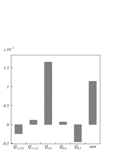
Figure 2: The $I=0$ and $I=2$ contributions to $\varepsilon^{\prime}/\varepsilon$ of the dominant operators using LO Wilson coefficients and the experimental phases. We also use the central values for $\Lambda_{\mbox{\tiny QCD}}$, $m_{s}(1\,\mbox{GeV})$, $\Omega_{\eta+\eta^{\prime}}$, and $\mbox{Im}\lambda_{t}$ at a scale of $\Lambda_{c}=700\,$MeV. The contributions of the operators $Q_{3}$ and $Q_{5}$ are negligible and are not included in the figure.

Figure 3: Various contributions to $\varepsilon^{\prime}/\varepsilon$ using LO Wilson coefficients and the experimental phases, plotted as functions of the matching scale $\Lambda_{c}$. We use central values for $m_{s}$, $\Omega_{\eta+\eta^{\prime}}$, $\Lambda_{\mbox{\tiny QCD}}$, and $\mbox{Im}\lambda_{t}$.

Figure 4: Same as in Fig. 1, now using NLO Wilson coefficients in the NDR scheme. The solid (dashed, dot-dashed) lines correspond to $\Lambda_{\mbox{\tiny QCD}}=\Lambda^{(4)}_{\overline{\mbox{\tiny MS}}}=325$ $(245,\,405)\,\,\mbox{MeV}$.

Figure 5: Same as in Fig. 3, now using NLO Wilson coefficients in the NDR scheme.

Figure 6: Same as in Fig. 3, now using NLO Wilson coefficients in the HV scheme.

Figure 7: Same as in Fig. 1, now using NLO Wilson coefficients in the HV scheme. The solid (dashed, dot-dashed) lines correspond to $\Lambda_{\mbox{\tiny QCD}}=\Lambda^{(4)}_{\overline{\mbox{\tiny MS}}}=325$ $(245,\,405)\,\,\mbox{MeV}$.

In Fig. 1 we depict $\varepsilon^{\prime}/\varepsilon$ as a function of the matching scale ($\mu=\Lambda_{c}$), calculated from Eqs. (43) and (44) with LO Wilson coefficients for the central value of $\mbox{Im}\lambda_{t}$ and for various values of $m_{s}$, $\Omega_{\eta+\eta^{\prime}}$, and $\Lambda_{\mbox{\tiny QCD}}$ according to their ranges defined above. For low values of the matching scale we find a rather moderate enhancement of the VSA result which is due to the weaker cancellation between the $Q_{6}$ and $Q_{8}$ operators. However, one might note that very large values for $\varepsilon^{\prime}/\varepsilon$ in the range of the recent Fermilab measurement [4] are not reached with the $B$ factors listed in Tabs. 3 and 4 together with Eq. (47), if central values are used for the parameters. Indeed, adopting central values for $m_{s}$, $\Omega_{\eta+\eta^{\prime}}$, $\Lambda_{\mbox{\tiny QCD}}$, and $\mbox{Im}\lambda_{t}$ and varying $\Lambda_{c}$ between 600 MeV and 900 MeV we obtain as ‘central range’ for the CP ratio:

$$8.4\cdot 10^{-4}\,\,\leq\,\,\varepsilon^{\prime}/\varepsilon\,\,(\mbox{LO-central})\,\,\leq\,\,12.9\cdot 10^{-4}\,.$$ (49)

This is also illustrated in Fig. 2 where we show the various contributions to $\varepsilon^{\prime}/\varepsilon$ for central values of the parameters at a scale of $\Lambda_{c}=700\,$MeV. For this value of the cutoff $B_{6}^{(1/2)}$ is very close to unity whereas $B_{8}^{(3/2)}$ is significantly suppressed which leads to a value for $\varepsilon^{\prime}/\varepsilon\,$ of $\,11.5\,\cdot 10^{-4}$. Smaller numbers are obtained for larger values of the cutoff. Another noticeable contribution, beside that of $Q_{8}$, which reduces the value of $\varepsilon^{\prime}/\varepsilon$ is the $I=0$ component of $Q_{1}$ and $Q_{2}$. As we already mentioned above, this contribution comes from the $Q_{4}$, $Q_{9}$, and $Q_{10}$ operators which are redundant below the charm threshold and satisfy, to LO and at NLO in the HV scheme, the relations in Eq. (66). In the NDR scheme the relations receive small ${\cal O}(\alpha_{s})$ and ${\cal O}(\alpha)$ corrections [10].

In Fig. 3 we show how the various terms depend on the choice of the matching scale. In particular, we observe that the behaviour of $\varepsilon^{\prime}/\varepsilon$ is almost identical to the one of $y_{6}\,\langle Q_{6}\rangle_{0}$. This is due to the fact that the ratio $B_{6}^{(1/2)}/B_{8}^{(3/2)}$ is approximately stable over the whole range of the cutoff $\Lambda_{c}$ and, consequently, $y_{6}\,\langle Q_{6}\rangle_{0}$ and $(-)\,y_{8}\,\langle Q_{8}\rangle_{2}$ fall off roughly in the same way. We note that the ratio $y_{6}(\mu)/m_{s}^{2}(\mu)$ increases by about $12\,\%$ if the scale $\mu=\Lambda_{c}$ is varied between $600\,$MeV and $1\,$GeV, whereas $B_{6}^{(1/2)}(\Lambda_{c})$ decreases by $44\,\%$. A similar statement applies to $Q_{8}$. The decrease of $B_{6}^{(1/2)}$ and $B_{8}^{(3/2)}$ is therefore qualitatively consistent with the (non-diagonal) evolution of $y_{6}$ and $y_{8}$ computed in the leading logarithmic approximation, and it leads to a fairly moderate overall scale dependence. This property is due to the fact that the ${\cal O}(p^{0}/N_{c})$ terms in Eqs. (39) and (40) have only a logarithmic cutoff dependence which, nevertheless, still goes beyond the $\mu$ dependence of the short-distance part. In this situation it would be tempting to adopt the large-$N_{c}$ values for $B_{6}^{(1/2)}$ and $B_{8}^{(3/2)}$ which are scale independent and coincide, to a very good approximation, with their VSA values $B_{6}^{(1/2)}=B_{8}^{(3/2)}=1$. However, the results show that $1/N_{c}$ corrections are important, and to recover the VSA values would require an a priori unexpected cancellation of the ${\cal O}(p^{0}/N_{c})$ corrections with higher order terms or contributions from higher resonances. Therefore, the VSA might underestimate the true range of uncertainty in the analysis of $\varepsilon^{\prime}/\varepsilon$.

The dependences of the result on $m_{s}$, $\Omega_{\eta+\eta^{\prime}}$, and $\Lambda_{\mbox{\tiny QCD}}$ are given in Fig. 1. Among them the $m_{s}$ dependence is the most important one. The dependence on Im$\lambda_{t}$, to a large degree of accuracy [27], is multiplicative and can be obtained in straightforward way. If we take into account the residual dependence on the matching scale by varying $\mu=\Lambda_{c}$ between $600$ and $900\,$MeV and scan independently the theoretical input parameters and the experimentally measured numbers, we obtain the following range for $\varepsilon^{\prime}/\varepsilon$ calculated with LO Wilson coefficients:

$$3.1\cdot 10^{-4}\,\,\leq\,\,\varepsilon^{\prime}/\varepsilon\,\,(\mbox{LO})\,\,\leq\,\,31.6\cdot 10^{-4}\,.$$ (50)

The quoted range results from a variation of $m_{s}$, $\Omega_{\eta+\eta^{\prime}}$, and $\Lambda_{\mbox{\tiny QCD}}$ in Eqs. (43) and (44) as depicted in Fig. 1 and also allows for a variation of $\mbox{Im}\lambda_{t}$ according to the range defined in Eq. (24).

We investigate next the dependence on the NLO Wilson coefficients. The NLO values are scheme dependent and are calculated within naive dimensional regularization (NDR) and in the ’t Hooft-Veltman scheme (HV), respectively. As already mentioned, the absence of any reference to the renormalization scheme dependence in the low-energy calculation prevents a complete matching at the next-to-leading order [22]. Nevertheless, a comparison of the numerical results obtained from the LO and NLO coefficients is useful in order to estimate the corresponding uncertainties and to test the validity of perturbation theory.

$$\begin{array}[]{|c||c|c|}\hline\cr&\mbox{Case}\,\,1&\mbox{Case}\,\,2\\ \hline\cr\hline\cr\rule{0.0pt}{14.22636pt}\mbox{LO}&\,\,8.4\,\,\leq\,\,\varepsilon^{\prime}/\varepsilon\,\,\leq\,\,12.9&\,\,6.3\,\,\leq\,\,\varepsilon^{\prime}/\varepsilon\,\,\leq\,\,9.5\\[1.42262pt] \mbox{NDR}&\,\,8.0\,\,\leq\,\,\varepsilon^{\prime}/\varepsilon\,\,\leq\,\,11.0&\,\,5.9\,\,\leq\,\,\varepsilon^{\prime}/\varepsilon\,\,\leq\,\,8.4\\[1.42262pt] \mbox{HV}&\,\,5.8\,\,\leq\,\,\varepsilon^{\prime}/\varepsilon\,\,\leq\,\,6.6&\,\,4.2\,\,\leq\,\,\varepsilon^{\prime}/\varepsilon\,\,\leq\,\,4.7\\[1.42262pt] \hline\cr\,\mbox{LO}\,+\,\mbox{NDR}\,+\,\mbox{HV}&\,\,5.8\,\,\leq\,\,\varepsilon^{\prime}/\varepsilon\,\,\leq\,\,12.9&\,\,4.2\,\,\leq\,\,\varepsilon^{\prime}/\varepsilon\,\,\leq\,\,9.5\\[1.42262pt] \hline\cr\end{array}$$

Table 5: Central ranges for $\varepsilon^{\prime}/\varepsilon$ (in units of $10^{-4}$) at LO and NLO (NDR and HV). The numbers are obtained for central values of $m_{s}$, $\Omega_{\eta+\eta^{\prime}}$, Im$\lambda_{t}$, and $\Lambda_{\mbox{\tiny QCD}}$ by varying $\Lambda_{c}$ between 600 and $900\,\mbox{MeV}$. ‘Case 1’ and ‘Case 2’ correspond to the use of Eqs. (43) - (44) and (45) - (46), respectively.

$$\begin{array}[]{|c||c|c|}\hline\cr&\mbox{Case}\,\,1&\mbox{Case}\,\,2\\ \hline\cr\hline\cr\rule{0.0pt}{14.22636pt}\mbox{LO}&\,\,3.1\,\,\leq\,\,\varepsilon^{\prime}/\varepsilon\,\,\leq\,\,31.6&\,\,2.4\,\,\leq\,\,\varepsilon^{\prime}/\varepsilon\,\,\leq\,\,23.2\\[1.42262pt] \mbox{NDR}&\,\,2.7\,\,\leq\,\,\varepsilon^{\prime}/\varepsilon\,\,\leq\,\,26.4&\,\,2.1\,\,\leq\,\,\varepsilon^{\prime}/\varepsilon\,\,\leq\,\,20.2\\[1.42262pt] \mbox{HV}&\,\,1.9\,\,\leq\,\,\varepsilon^{\prime}/\varepsilon\,\,\leq\,\,16.5&\,\,1.5\,\,\leq\,\,\varepsilon^{\prime}/\varepsilon\,\,\leq\,\,11.9\\[1.42262pt] \hline\cr\,\mbox{LO}\,+\,\mbox{NDR}\,+\,\mbox{HV}&\,\,1.9\,\,\leq\,\,\varepsilon^{\prime}/\varepsilon\,\,\leq\,\,31.6&\,\,1.5\,\,\leq\,\,\varepsilon^{\prime}/\varepsilon\,\,\leq\,\,23.2\\[1.42262pt] \hline\cr\end{array}$$

Table 6: Same results as in Tab. 5 but for the complete scanning of the parameters ($\Lambda_{c}$, $m_{s}$, $\Omega_{\eta+\eta^{\prime}}$ and $\Lambda_{\mbox{\tiny QCD}}$, and Im$\lambda_{t}$) as explained in the text.

In the NDR scheme, introducing the NLO coefficients does not noticeably affect our numerical results (see Fig. 4). For $\Lambda^{(4)}_{\overline{\mbox{\tiny MS}}}=\Lambda_{\mbox{\tiny QCD}}\lesssim 325\,\mbox{MeV}$ we find slightly lower values for $\varepsilon^{\prime}/\varepsilon$ and a somewhat larger difference between the results obtained for $\Lambda_{\mbox{\tiny QCD}}=325\,\mbox{MeV}$ and $405\,\mbox{MeV}$, respectively. Generally, the difference between LO and NLO is more pronounced for very low values of the matching scale, but it is still moderate except for $\Lambda_{\mbox{\tiny QCD}}=405\,\mbox{MeV}$. For $\Lambda_{\mbox{\tiny QCD}}=325\,\mbox{MeV}$ ($245\,\mbox{MeV}$) the effect of the NLO coefficients is rather small, and values for the matching scale as low as $600\,$-$\,700\,\mbox{MeV}$ appear to be acceptable. We also notice a slightly smaller scale dependence, that is to say, the NLO Wilson coefficients further improve the stability of the calculation. This property becomes obvious if we investigate the various contributions to $\varepsilon^{\prime}/\varepsilon$ (compare Figs. 3 and 5). In particular, at NLO in the NDR scheme we observe a smaller variation of $y_{6}\,\langle Q_{6}\rangle_{0}$ and $y_{8}\,\langle Q_{8}\rangle_{2}$ in the range of $\Lambda_{c}$ between $600\,\mbox{MeV}$ and $1\,\mbox{GeV}$. Nevertheless, the numerical effect of the NLO coefficients is rather moderate, and the ‘central’ and scanned ranges quoted in Tabs. 5 and 6 are close to the LO results given in Eqs. (49) and (50).

In the HV scheme, the effect of the NLO coefficients is more pronounced. Both $y_{6}\,\langle Q_{6}\rangle_{0}$ and $y_{8}\,\langle Q_{8}\rangle_{2}$ are rather stable over a large range of the matching scale leading to an approximately stable result for $\varepsilon^{\prime}/\varepsilon$ between $700\,\mbox{MeV}$ and $1\,\mbox{GeV}$. This is shown in Fig. 6 for the central values of $m_{s}(1\,\mbox{GeV})$, $\Omega_{\eta+\eta^{\prime}}$, $\mbox{Im}\lambda_{t}$, and $\Lambda_{\mbox{\tiny QCD}}$. On the other hand, for $\Lambda_{\mbox{\tiny QCD}}=405\,\mbox{MeV}$ and $\Lambda_{c}\lesssim 700\,\mbox{MeV}$ we observe a noticeable slope indicating the breakdown of the perturbative expansion of QCD (see Fig. 7). However, for moderate values of the matching scale the numerical values for the ratio depend weakly on the choice of $\Lambda_{\mbox{\tiny QCD}}$ (see Fig. 7), which makes the result rather stable. Generally, at NLO in the HV scheme we obtain smaller values for $\varepsilon^{\prime}/\varepsilon$ (see Tabs. 5 and 6).

We note that at NLO the maximum value for the ratio is found for moderate values of $\Lambda_{c}$ around $700\,$-$\,800\,\mbox{MeV}$, whereas the upper bound in Eq. (50) refers to low values of the matching scale ($\sim 600\,\mbox{MeV}$). Finally, one might note that the numerical values of the Wilson coefficients in the HV scheme communicated to us by M. Jamin [43] correspond to the treatment of the two-loop anomalous dimensions used in Ref. [10] which differs from the one used in Ref. [11]. For this reason the NLO corrections to the Wilson coefficients in the HV scheme presented in Appendix A are generally smaller than the ones found in Ref. [11] (for a discussion of this point see also Ref. [22]).

So far in the numerical analysis we have used Eqs. (43) - (44) together with the phenomenological values for the phases [48]. Replacing them by Eqs. (45) - (46) leads to lower values for $\varepsilon^{\prime}/\varepsilon$ (see Case  2 in Tabs. 5 and 6). The numerical results are very close to those we would get if we used the imaginary parts obtained at the one-loop level in the $1/N_{c}$ approach. Both the central values and the upper bounds in the scanned ranges for $\varepsilon^{\prime}/\varepsilon$ are lower due to a smaller contribution from the $\Delta I=1/2$ terms. However, the modifications do not change substantially our picture of $\varepsilon^{\prime}/\varepsilon$. As mentioned above, the comparison of the two cases provides, in part, an estimate for higher order effects.

In conclusion, the fact that we use rather low values for the matching scale makes some of the Wilson coefficients rather sensitive to NLO corrections. In particular, $y_{6}$ and $y_{8}$ depend noticeably on the choice of the $\gamma_{5}$ scheme in dimensional regularization. For example, for $\mu=700\,\mbox{MeV}$ and $\Lambda_{\mbox{\tiny QCD}}=325\,$MeV the values of $y_{6}$ and $y_{8}$ at LO and in the NDR and HV schemes differ approximately by 20 - 30 %. Since the non-perturbative calculation of the matrix elements is insensitive to this dependence, the corresponding uncertainty must be included in the final result for $\varepsilon^{\prime}/\varepsilon$. Collecting together the LO and NLO values in Tab. 5 from Eqs. (43) - (44) and (45) - (46) we get the following range:

$$4.2\cdot 10^{-4}\,\,\leq\,\,\varepsilon^{\prime}/\varepsilon\,\,(\mbox{central})\,\,\leq\,\,12.9\cdot 10^{-4}\,,$$ (53)

which, for central values of $m_{s}$, $\Omega_{\eta+\eta^{\prime}}$, $\Lambda_{\mbox{\tiny QCD}}$, and Im$\lambda_{t}$, takes into account the theoretical errors inherent to the method (dependence on the scheme and matching scale). Furthermore, it includes the expected errors due to the neglect of higher order corrections to the imaginary part. Similarly collecting the values in Tab. 6 we obtain the following range from the complete scanning of the parameters:

$$1.5\cdot 10^{-4}\,\,\leq\,\,\varepsilon^{\prime}/\varepsilon\,\,\leq\,\,31.6\cdot 10^{-4}\,,$$ (54)

which also takes into account the uncertainties in the values for $m_{s}$, $\Omega_{\eta+\eta^{\prime}}$, $\Lambda_{\mbox{\tiny QCD}}$, and Im$\lambda_{t}$. The upper bound from our calculation in Eq. (54) is rather close to the central value of the new Fermilab measurement [4] and requires a conspiracy of the parameters within their ranges of uncertainties given above.

The present world average for the ratio including earlier measurements is $\mbox{Re}(\varepsilon^{\prime}/\varepsilon)=(21.8\pm 3.0)\cdot 10^{-4}$ [4]. Our result indicates that the experimental data can be accommodated in the standard model. A major uncertainty in the theoretical estimate of $\varepsilon^{\prime}/\varepsilon$ is due to the choice of $m_{s}$, which enters the calculation through the matrix elements of the operators $Q_{6}$ and $Q_{8}$ [see Eqs. (39) and (40)]. In Eq. (54) we have taken $m_{s}(1\,\mbox{GeV})=150\pm 25\,\mbox{MeV}$ which is in the range of the values obtained in quenched lattice calculations and from the QCD sum rules. Adopting even lower values for $m_{s}$ would allow us to relax the upper bound quoted above. However, recently the ALEPH collaboration analyzed the measured mass spectra of the strange $\tau$ decay modes and reported a value of $m_{s}(1\,\mbox{GeV})=234{+61\atop-76}\,\mbox{MeV}$ [53]. It will be interesting to see whether this large (central) value for $m_{s}$ will remain when the error is reduced. Very recently, the value $m_{s}(1\,\mbox{GeV})=(188\pm 22)\,$MeV was obtained using a $\tau$-like decay sum rule for the $\phi$ meson [54], which is consistent with the range used in this paper. The determination of $\mbox{Im}\lambda_{t}$ will be further improved by precision tests of the unitarity triangle [22] removing to a large extent the corresponding uncertainty in the analysis of direct CP violation. $\Omega_{\eta+\eta^{\prime}}$ which measures the contribution to $\varepsilon^{\prime}/\varepsilon$ from the isospin breaking in the quark masses was estimated in Ref. [16] in the large-$N_{c}$ limit, and it will be a challenge to investigate, in future studies, the $1/N_{c}$ corrections to this parameter. Finally, the calculation of the hadronic matrix elements even though largely improved by including $1/N_{c}$ corrections may still be plagued by noticeable uncertainties. Our analysis so far included terms of ${\cal O}(p^{0})$, ${\cal O}(p^{0}/N_{c})$, and ${\cal O}(p^{2})$ for the matrix elements of the density-density operators and terms of ${\cal O}(p^{2})$, ${\cal O}(p^{2}/N_{c})$, and ${\cal O}(p^{4})$ for the matrix elements of the current-current operators. In the following section we shall investigate the effect of higher order corrections. In particular we will consider the terms of ${\cal O}(p^{2}/N_{c})$ for the matrix elements of $Q_{6}$.

5 Higher Order Corrections

In the previous section we have shown that the calculation of the hadronic matrix elements in the $1/N_{c}$ expansion leads to a well defined range of values for $\varepsilon^{\prime}/\varepsilon$ which can account, to a large extent, for the weighted average of the experimental measurements [2, 3, 4]. However, the central values obtained are lower than the values of the new measurement [4]. The upper bound from our calculation requires, within the standard model, specific values of various parameters. In particular, lower values of the strange quark mass are favoured. In our analysis so far we varied the theoretical input parameters independent of each other and considered the experimental results within one standard deviation. This conservative attitude may to some extent exaggerate the differences [55]. In the present section we investigate the higher order corrections and consider in particular the question whether these corrections are able to substantially enhance the prediction for $\varepsilon^{\prime}/\varepsilon$, so that a large value for the ratio could be explained even for central values of the input parameters.

In the twofold expansion, the higher order corrections to the matrix elements of $Q_{6}$ and $Q_{8}$ are of orders: ${\cal O}(p^{4})$, ${\cal O}(p^{0}/N_{c}^{2})$, and ${\cal O}(p^{2}/N_{c})$. In this section we will consider the ${\cal O}(p^{2}/N_{c})$ contribution which brings in, for the first time, quadratic corrections on the cutoff. From general counting arguments we show that these corrections are expected to be large for $Q_{6}$, which is a peculiar operator. $Q_{6}$ is consequently not protected from possible large corrections beyond the large-$N_{c}$ limit, and we cannot exclude the possibility that the contribution of $Q_{6}$ brings $\varepsilon^{\prime}/\varepsilon$ close to the experimental value for central values of the parameters. Calculating the ${\cal O}(p^{2}/N_{c})$ correction for $Q_{6}$ in the chiral limit we explicitly find that it is indeed large and positive.

Before investigating the ${\cal O}(p^{2}/N_{c})$ corrections we briefly estimate part of the higher order corrections replacing the ‘$1/F_{\pi}$ expansion’ by a ‘$1/F_{K}$ expansion’. As already discussed in Ref. [14], we could have used the ratio $1/f$ in place of $1/F_{\pi}$ in the next-to-leading order terms of Eqs. (37) - (40). This choice would be consistent at the level of first order corrections in the twofold series expansion, as the difference concerns higher order effects. However, the scale dependence of $f$ (which is mainly quadratic) is absorbed through the factorizable loops to the matrix elements at the next order in the parameter expansion and does not occur in the matching with the short-distance contribution [14]. Consequently, it is more appropriate to choose the physical decay constant in the expressions under consideration. In this situation, we can use, instead of $F_{\pi}$, the kaon decay constant $F_{K}$ which gives an indirect estimate of higher order corrections. In Tab. 7 we show the effect of this modification, to ${\cal O}(p^{0}/N_{c})$, on the values of $B_{6}^{(1/2)}$ and $B_{8}^{(3/2)}$. We notice that the numbers are generally larger for the ‘$1/F_{K}$ expansion’. In particular, for $\Lambda_{c}\lesssim 900\,\mbox{MeV}$ the $B_{6}^{(1/2)}$ factor is enhanced compared to the VSA value. This change, in spite of the somewhat smaller reduction of $B_{8}^{(3/2)}$, leads to a moderate enhancement of $\varepsilon^{\prime}/\varepsilon$ which further improves the agreement with the observed value. Numerically, collecting together the various terms we get $5.3\cdot 10^{-4}\,\leq\,\varepsilon^{\prime}/\varepsilon\,(\mbox{central})\,\leq\,15.8\cdot 10^{-4}$. Scanning independently the input parameters we obtain $1.8\cdot 10^{-4}\,\leq\,\varepsilon^{\prime}/\varepsilon\,\leq\,38.3\cdot 10^{-4}$ in place of Eq. (54). Adopting zero phases reduces the upper bound to $28.3\cdot 10^{-4}$.

$$\begin{array}[]{|c||c|c|c|c|c|c|}\hline\cr\Lambda_{c}&0.6\,\,\mbox{GeV}&0.7\,\,\mbox{GeV}&0.8\,\,\mbox{GeV}&0.9\,\,\mbox{GeV}&1.0\,\,\mbox{GeV}\\ \hline\cr\hline\cr\rule{0.0pt}{14.22636pt}B_{6}^{(1/2)}&1.10&0.96&0.84&0.72&0.62\\ &(1.30)&(1.19)&(1.09)&(0.99)&(0.91)\\[1.42262pt] B_{8}^{(3/2)}&0.64&0.56&0.49&0.42&0.34\\ &(0.72)&(0.66)&(0.59)&(0.53)&(0.46)\\[1.42262pt] \hline\cr\end{array}$$

Table 7: Bag parameters $B_{6}^{(1/2)}$ and $B_{8}^{(3/2)}$ shown for various values of $\Lambda_{c}$. The numbers in the parentheses are obtained by replacing $F_{\pi}$ by $F_{K}$ in the next-to-leading order expression.

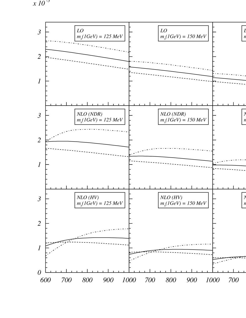
Figure 8: $\varepsilon^{\prime}/\varepsilon$ using LO and NLO (NDR and HV) Wilson coefficients and the experimental phases, plotted for various values of $m_{s}$ as a function of the matching scale $\Lambda_{c}=\mu$, now with $1/F_{\pi}\rightarrow 1/F_{K}$ in the next-to-leading order terms for the matrix elements. We use the central values for $\mbox{Im}\lambda_{t}$ and $\Omega_{\eta+\eta^{\prime}}$. The solid (dashed, dot-dashed) lines correspond to $\Lambda_{\mbox{\tiny QCD}}=325$ $(245,\,405)\,\,\mbox{MeV}$.

In Fig. 8 we depict $\varepsilon^{\prime}/\varepsilon$ as a function of the matching scale ($\mu=\Lambda_{c}$), calculated with LO and NLO (NDR and HV) Wilson coefficients and for the central values of $\mbox{Im}\lambda_{t}$ and $\Omega_{\eta+\eta^{\prime}}$ and various values of $m_{s}$. The variation of $\Omega_{\eta+\eta^{\prime}}$ does not change the qualitative behaviour; it only shifts the curves upward or downward for smaller or larger values of $\Omega_{\eta+\eta^{\prime}}$, respectively. The curves in Fig. 8 result from replacing $1/F_{\pi}$ by $1/F_{K}$ in all next-to-leading order expressions relevant to the complete set of matrix elements. Beside the enhancement of the numerical result we also observe a somewhat smaller dependence on the matching scale. Finally, even though we obtain somewhat larger values for $\varepsilon^{\prime}/\varepsilon$ the effect is still rather moderate and does not affect the statement we made above that lower values of the strange quark mass are favoured.

In the above we have argued that estimating the effect of higher order corrections to the matrix elements, by replacing the ‘$1/F_{\pi}$ expansion’ by a ‘$1/F_{K}$ expansion’, does not drastically modify the results we obtained in the previous section. In particular, this statement refers to terms of ${\cal O}(p^{0}/N_{c}^{2})$ which are corrections on top of the ${\cal O}(p^{0}/N_{c})$ contribution and correspond to the same pseudoscalar representation of the four-quark operator. In the following we will not study the $1/N_{c}^{2}$ corrections, which correspond to a two-loop diagram in the chiral theory. The same approximation was made in the chiral quark model [46]. However, estimating the typical effect of higher orders by modifying the known corrections ($1/F_{\pi}\rightarrow 1/F_{K}$) does not account for possible contributions from new terms which are absent at the level of the first order corrections. In particular, higher order terms in the $p^{2}$ expansion (tree level) cannot be calculated because the low-energy couplings in the ${\cal O}(p^{6})$ lagrangian are very uncertain or even unknown. Nevertheless, these terms are independent of the (non-factorizable) matching scale and are chirally suppressed with respect to the leading term ($\sim m_{K,\pi}^{2}/\Lambda_{\chi}^{2}$, with $\Lambda_{\chi}\simeq 1\,\mbox{GeV}$ the scale of chiral symmetry breaking). The convergence of the tree level series was verified for the current-current operators [13, 29] and also for $Q_{8}$ [14], where a complete leading plus next-to-leading order calculation now exists and tree contributions appear to decrease monotonically. For the operator $Q_{6}$ the leading term is ${\cal O}(p^{2})$ and by analogy we expect the higher order tree terms to be smaller. The terms of ${\cal O}(p^{2}/N_{c})$ on the other hand are not expected to be small for $Q_{6}$. We remind the readers that for the CP conserving amplitude it is mainly the (quadratic) ${\cal O}(p^{2}/N_{c})$ corrections which bring to $\langle Q_{1,2}\rangle_{0}$ a large enhancement relative to the (leading-$N_{c}$) ${\cal O}(p^{2})$ values. As the leading-$N_{c}$ value for $Q_{6}$ is also ${\cal O}(p^{2})$ we cannot a priori exclude that the value of $\langle Q_{6}\rangle_{0}$ is largely affected by ${\cal O}(p^{2}/N_{c})$ corrections too. As already discussed in Section 4.1, quadratic ${\cal O}(p^{2}/N_{c})$ corrections are proportional to the factor $\Delta\equiv\Lambda_{c}^{2}/(4\pi F_{\pi})^{2}$ relative to the ${\cal O}(p^{2})$ tree level contribution. Different is the case of the operator $Q_{8}$ since its leading-$N_{c}$ value is ${\cal O}(p^{0})$ at lowest order in the chiral expansion. Quadratic terms for $Q_{8}$ are consequently chirally suppressed with respect to the leading-$N_{c}$ value. More precisely the suppression factor is $\sim(m_{K,\pi}^{2}/\Lambda_{\chi}^{2})\cdot\Delta$. In contrast to $\langle Q_{6}\rangle_{0}$, it is very unlikely that the ${\cal O}(p^{2}/N_{c})$ corrections for $\langle Q_{8}\rangle_{2}$ could be larger than the ${\cal O}(p^{0}/N_{c})$ contributions investigated in the previous section.

We calculate next the ${\cal O}(p^{2}/N_{c})$ quadratic corrections to the matrix elements of the operator $Q_{6}$. The pseudoscalar representation of $Q_{6}$ can be read off from Eq. (30):

$$Q_{6} = -2f^{2}r^{2}\sum_{q}\Bigg{[}\frac{1}{4}f^{2}(U^{\dagger})_{dq}(U)_{qs}+(U^{\dagger})_{dq}\big{(}L_{5}U\partial_{\mu}U^{\dagger}\partial^{\mu}U+2rL_{8}U{\cal M}^{\dagger}U$$ (56)

$$+rH_{2}{\cal M}\big{)}_{qs}+\big{(}L_{5}U^{\dagger}\partial_{\mu}U\partial^{\mu}U^{\dagger}+2rL_{8}U^{\dagger}{\cal M}U^{\dagger}+rH_{2}{\cal M}^{\dagger}\big{)}_{dq}(U)_{qs}\Bigg{]}+{\cal O}(p^{4})\,.\hskip 18.49428pt$$

In the following we will calculate the ${\cal O}(p^{2}/N_{c})$ evolution of the operator $Q_{6}$ in the chiral limit. It is then straightforward to compute the hadronic matrix element $\langle Q_{6}\rangle_{0}$. To calculate the evolution of $Q_{6}$ we use the background field method as described in Ref. [39] and also in Refs. [14, 40]. This operatorial method is very convenient to calculate corrections in the chiral limit. To this end we decompose the matrix $U$ in the classical field $\bar{U}$ and the quantum fluctuation $\xi$,

$$U=\exp(i\sqrt{2}\xi/f)\,\bar{U}\;,\hskip 14.22636pt\xi=\xi^{a}\frac{\lambda_{a}}{\sqrt{2}}\,,$$ (57)

with $\bar{U}$ satisfying the equation of motion

$$\bar{U}\partial^{2}\bar{U}^{\dagger}-\partial^{2}\bar{U}\bar{U}^{\dagger}+r\bar{U}{\cal M}^{\dagger}-r{\cal M}\bar{U}^{\dagger}=\frac{\alpha}{N_{c}}\langle\ln\bar{U}-\ln\bar{U}^{\dagger}\rangle\cdot{\bf 1}\;,\hskip 14.22636pt\bar{U}=\exp(i\pi^{a}\lambda_{a}/f)\;.$$ (58)

The ${\cal O}(p^{2})$ lagrangian thus reads

$${\cal L}=\bar{\cal L}+\frac{1}{2}(\partial_{\mu}\xi^{a}\partial^{\mu}\xi_{a})+\frac{1}{2}\langle[\partial_{\mu}\xi,\,\xi]\partial^{\mu}\bar{U}\bar{U}^{\dagger}\rangle-\frac{r}{4}\langle\xi^{2}\bar{U}{\cal M}^{\dagger}+\bar{U}^{\dagger}\xi^{2}{\cal M}\rangle-\frac{1}{2}\alpha\xi^{0}\xi^{0}+{\cal O}(\xi^{3})\;.$$ (59)

The corresponding expansion of the meson density in Eq. (30) around the classical field yields

$$(D_{L})_{ij} \equiv \bar{q}_{iR}q_{jL}\,\,=\,\,(\bar{D}_{L})_{ij}+irf\frac{\sqrt{2}}{4}(\bar{U}^{\dagger}\xi)_{ji}+\frac{r}{4}(\bar{U}^{\dagger}\xi^{2})_{ji}\,$$ (60)

$$+\,\,i\frac{r}{f}L_{5}\sqrt{2}\,\big{[}\,\partial^{\mu}\bar{U}^{\dagger}\partial_{\mu}\bar{U}\bar{U}^{\dagger}\xi+\bar{U}^{\dagger}\{\partial^{\mu}\xi,\partial_{\mu}\bar{U}\bar{U}^{\dagger}\}\,\big{]}_{ji}\,$$

$$-\,\,\frac{r}{f^{2}}L_{5}\,\big{[}\,2\bar{U}^{\dagger}\partial^{\mu}\xi\partial_{\mu}\xi+\bar{U}^{\dagger}[\partial^{\mu}\xi,\xi]\partial_{\mu}\bar{U}\bar{U}^{\dagger}\,$$

$$-\,\,2\bar{U}^{\dagger}\partial^{\mu}\xi\partial_{\mu}\bar{U}\bar{U}^{\dagger}\xi+\partial^{\mu}\bar{U}^{\dagger}\{\partial_{\mu}\xi,\xi\}-\partial^{\mu}\bar{U}^{\dagger}\partial_{\mu}\bar{U}\bar{U}^{\dagger}\xi^{2}\,\big{]}_{ji}\,$$

$$+\,\,i2\sqrt{2}\,\frac{r^{2}}{f}L_{8}\,[\,\bar{U}^{\dagger}\{\xi,{\cal M}\bar{U}^{\dagger}\}\,]_{ji}\,+2\,\frac{r^{2}}{f^{2}}L_{8}\,[\,\bar{U}^{\dagger}\{\xi^{2},{\cal M}\bar{U}^{\dagger}\}\,]_{ji}\,+{\cal O}(\xi^{3})\,.\hskip 22.76219pt$$

Using Eq. (60) the evolution of $Q_{6}$ can be obtained in a straightforward way. Integrating over the quantum fluctuation by calculating the non-factorizable diagrams of Fig. 9.a we get the following result:

$$Q_{6}(\Lambda_{c}^{2})=-4F_{\pi}^{2}r^{2}\hat{L}_{5}^{r}(\partial^{\mu}\bar{U}^{\dagger}\partial_{\mu}\bar{U})_{ds}\,\Bigg{[}1+\frac{3}{2}\frac{\Lambda_{c}^{2}}{(4\pi F_{\pi})^{2}}\Bigg{]}\,.$$ (61)

This result has already been presented in Ref. [40]. Before investigating the numerical effect of the quadratic term in Eq. (61) a few comments are necessary:

• In Eq. (61) we present only the diagonal evolution, i.e., the term proportional to the operator $(\partial^{\mu}\bar{U}^{\dagger}\partial_{\mu}\bar{U})_{ds}$ which gives the only non-vanishing contribution to the $K\rightarrow\pi\pi$ amplitudes. This property is analogous to the tree level. One might note in particular that the $L_{8}$ contribution vanishes since it does not produce a term proportional to this operator. The $H_{2}$ contribution vanishes from the beginning as it does not appear in Eq. (60).

• To ${\cal O}(p^{0}/N_{c})$ we showed explicitly that the factorizable contributions provide the corrections needed to obtain the physical values of the low-energy couplings [14]. Except for finite corrections, the values of the couplings can be obtained in the large-$N_{c}$ limit, i.e., by imposing tree level relations in order to set up the renormalized (factorizable) matrix elements [compare Eqs. (41) and (42)]. To ${\cal O}(p^{2}/N_{c})$ in Eq. (61) we use again the renormalized coupling $\hat{L}_{5}^{r}$, defined in the large-$N_{c}$ limit, since the scale dependence of the bare coefficient $L_{5}$ will be absorbed in factorizable loop corrections to the matrix elements and does not need to be matched to any short-distance contribution [14].

• Beside the diagrams in Fig. 9.a a priori the diagram in Fig. 9.b with a strong vertex proportional to $L_{5}$ could also contribute. However, it is easy to see that since the $L_{5}$ term in the lagrangian contains a quark mass matrix ${\cal M}$, this diagram produces an operator similar to the one resulting from the $L_{8}$ term at tree level for $Q_{6}$. This operator does not contribute to the $K\rightarrow\pi\pi$ amplitudes.

• The diagram of Fig. 9.b with the strong vertex coming from the $L_{1}$, $L_{2}$, $L_{3}$, and $L_{8}$ couplings also turns out to vanish.

• There are no ${\cal O}(p^{2}/N_{c})$ tree level contributions, i.e., from couplings $L_{i}$ [33] which are subleading in $N_{c}$.

Figure 9: Non-factorizable loop diagrams for the evolution of $Q_{6}$ to ${\cal O}(p^{2}/N_{c})$. The crossed circles denote the two bosonized densities, the black circles the strong interaction vertices from the kinetic term in the lagrangian. Similar diagrams with the ${\cal O}(p^{2})$ mass or $U_{A}(1)$ terms in Eq. (59) are logarithmically divergent or finite, and we do not present them here.

Numerically, we observe a large positive correction from the quadratic term of ${\cal O}(p^{2}/N_{c})$ in Eq. (61). The slope of this correction is qualitatively consistent and welcome since it compensates for the logarithmic decrease at ${\cal O}(p^{0}/N_{c})$. Adding the ${\cal O}(p^{2}/N_{c})$ term to the full ${\cal O}(p^{2})$ and ${\cal O}(p^{0}/N_{c})$ result in Eq. (39) we obtain the following matrix element for $Q_{6}$:

$$\langle Q_{6}\rangle_{0}=-\frac{4\sqrt{3}}{F_{\pi}}R^{2}(m_{K}^{2}-m_{\pi}^{2})\left[\hat{L}_{5}^{r}\left(1+\frac{3}{2}\frac{\Lambda_{c}^{2}}{(4\pi)^{2}F_{\pi}^{2}}\right)-\frac{3}{16\,(4\pi)^{2}}\,\log\Lambda_{c}^{2}\,+\,\cdots\,\right].\hskip 14.22636pt$$ (62)

$$\begin{array}[]{|c||c|c|c|c|c|c|}\hline\cr\Lambda_{c}&0.6\,\,\mbox{GeV}&0.7\,\,\mbox{GeV}&0.8\,\,\mbox{GeV}&0.9\,\,\mbox{GeV}&1.0\,\,\mbox{GeV}\\ \hline\cr\hline\cr\rule{0.0pt}{14.22636pt}B_{6}^{(1/2)}&1.50&1.51&1.55&1.62&1.73\\[1.42262pt] \hline\cr\end{array}$$

Table 8: $B_{6}^{(1/2)}$, now including, in the chiral limit, terms of ${\cal O}(p^{2}/N_{c})$.

The corresponding values of $B_{6}^{(1/2)}$ (obtained by adding the quadratic corrections to the values in Tab. 3) are listed in Tab. 8. The $B_{6}^{(1/2)}$ factor is found to be rather stable around the value $B_{6}^{(1/2)}\simeq 1.6\pm 0.1$. The quadratic term of ${\cal O}(p^{2}/N_{c})$ is of the same magnitude as the ${\cal O}(p^{2})$ tree term. For the $\langle Q_{1}\rangle_{0}$ and $\langle Q_{2}\rangle_{0}$ there was also a large enhancement to the ${\cal O}(p^{2})$ tree contribution introduced by the ${\cal O}(p^{2}/N_{c})$ term (see Tabs. 1 and 3). $Q_{6}$ is a $\Delta I=1/2$ operator, and the enhancement of $\langle Q_{6}\rangle_{0}$ suggests that at the level of the $1/N_{c}$ corrections the dynamics of the $\Delta I=1/2$ rule also applies to $Q_{6}$. One might however note that the long-distance evolution of the operator $Q_{6}$ including both the ${\cal O}(p^{0}/N_{c})$ and ${\cal O}(p^{2}/N_{c})$ terms is very different from the one of $Q_{1}$ or $Q_{2}$. The former is approximately constant over a wide range of the cutoff scale due to the smaller coefficient of the quadratic term and a large cancellation of the scale dependences between the quadratic and the logarithmic term, whereas the later [which does not receive any ${\cal O}(p^{0}/N_{c})$ contribution] has a large positive slope. One should also remark that we observe a noticeable suppression of $\langle Q_{8}\rangle_{2}$ similar to the one needed for $\langle Q_{1,2}\rangle_{2}$ in order to bring the CP conserving $\Delta I=3/2$ amplitude down to the experimental value.

Using the values for $B_{6}^{(1/2)}$ in Tab. 8 together with the bag factors of the remaining operators presented in the previous section we calculated again the ratio $\varepsilon^{\prime}/\varepsilon$ for central values of $m_{s}$, $\Omega_{\eta+\eta^{\prime}}$, Im$\lambda_{t}$, and $\Lambda_{\mbox{\tiny QCD}}$. The results for the three sets of Wilson coefficients LO, NDR, and HV and for $\Lambda_{c}$ between 600 and $900\,\mbox{MeV}$ are given in Tab. 9. The numbers are obtained from Eqs. (43) - (44) and (45) - (46), respectively. With LO Wilson coefficients, the enhancement of $B_{6}^{(1/2)}$ leads to larger values for $\varepsilon^{\prime}/\varepsilon$, and the predictions are now more stable and closer to the data. The results in the NDR scheme are rather close to the LO ones although more sensitive to the value of $\Lambda_{\mbox{\tiny QCD}}$. In the HV scheme, the effect of the NLO coefficients is more pronounced. The results are significantly smaller for low values of the matching scale and less stable. This is illustrated in Fig. 10 where we show $\varepsilon^{\prime}/\varepsilon$ for various values of $m_{s}$ as a function of the matching scale.

Performing a scanning of the input parameters as explained above, we arrive at the values in Tab. 10. Comparing these results with the values in Tabs. 5 and 6 we see a clear enhancement originating from the quadratic term in Eq. (62). The large ranges reported in Tab. 10 can be traced back to the large ranges of the input parameters. The parameters, to a large extent, act multiplicatively, and the larger range for $\varepsilon^{\prime}/\varepsilon$ is due to the fact that the central value(s) for the ratio are enhanced roughly by a factor of two compared to the results we presented in the previous section. More accurate information on the parameters, from theory and experiment, will restrict the values for the CP ratio.

$$\begin{array}[]{|c||c|c|}\hline\cr&\mbox{Case}\,\,1&\mbox{Case}\,\,2\\ \hline\cr\hline\cr\rule{0.0pt}{14.22636pt}\mbox{LO}&\,\,19.5\,\,\leq\,\,\varepsilon^{\prime}/\varepsilon\,\,\leq\,\,24.7&\,\,14.8\,\,\leq\,\,\varepsilon^{\prime}/\varepsilon\,\,\leq\,\,19.4\\[1.42262pt] \mbox{NDR}&\,\,16.1\,\,\leq\,\,\varepsilon^{\prime}/\varepsilon\,\,\leq\,\,23.4&\,\,12.5\,\,\leq\,\,\varepsilon^{\prime}/\varepsilon\,\,\leq\,\,18.3\\[1.42262pt] \mbox{HV}&\,\,9.3\,\,\,\,\leq\,\,\varepsilon^{\prime}/\varepsilon\,\,\leq\,\,19.3&\,\,7.0\,\,\,\,\leq\,\,\varepsilon^{\prime}/\varepsilon\,\,\leq\,\,14.9\\[1.42262pt] \hline\cr\,\mbox{LO}\,+\,\mbox{NDR}\,+\,\mbox{HV}&\,\,9.3\,\,\,\,\leq\,\,\varepsilon^{\prime}/\varepsilon\,\,\leq\,\,24.7&\,\,7.0\,\,\,\,\leq\,\,\varepsilon^{\prime}/\varepsilon\,\,\leq\,\,19.4\\[1.42262pt] \hline\cr\end{array}$$

Table 9: Same results as in Tab. 5, but now including quadratic terms of ${\cal O}(p^{2}/N_{c})$ for $Q_{6}$ as explained in the text.

$$\begin{array}[]{|c||c|c|}\hline\cr&\mbox{Case}\,\,1&\mbox{Case}\,\,2\\ \hline\cr\hline\cr\rule{0.0pt}{14.22636pt}\mbox{LO}&\,\,8.0\,\,\leq\,\,\varepsilon^{\prime}/\varepsilon\,\,\leq\,\,62.1&\,\,6.1\,\,\leq\,\,\varepsilon^{\prime}/\varepsilon\,\,\leq\,\,48.5\\[1.42262pt] \mbox{NDR}&\,\,6.8\,\,\leq\,\,\varepsilon^{\prime}/\varepsilon\,\,\leq\,\,63.9&\,\,5.2\,\,\leq\,\,\varepsilon^{\prime}/\varepsilon\,\,\leq\,\,49.8\\[1.42262pt] \mbox{HV}&\,\,2.8\,\,\leq\,\,\varepsilon^{\prime}/\varepsilon\,\,\leq\,\,49.8&\,\,2.2\,\,\leq\,\,\varepsilon^{\prime}/\varepsilon\,\,\leq\,\,38.5\\[1.42262pt] \hline\cr\,\mbox{LO}\,+\,\mbox{NDR}\,+\,\mbox{HV}&\,\,2.8\,\,\leq\,\,\varepsilon^{\prime}/\varepsilon\,\,\leq\,\,63.9&\,\,2.2\,\,\leq\,\,\varepsilon^{\prime}/\varepsilon\,\,\leq\,\,49.8\\[1.42262pt] \hline\cr\end{array}$$

Table 10: Same results as in Tab. 6, but now including quadratic terms of ${\cal O}(p^{2}/N_{c})$ for $Q_{6}$ as explained in the text.

Figure 10: $\varepsilon^{\prime}/\varepsilon$ using LO and NLO (NDR and HV) Wilson coefficients and the experimental phases, plotted for various values of $m_{s}$ as a function of the matching scale $\Lambda_{c}=\mu$, including for $Q_{6}$ the term of ${\cal O}(p^{2}/N_{c})$ in the chiral limit. We use again the values $\mbox{Im}\lambda_{t}=1.33\cdot 10^{-4}$ and $\Omega_{\eta+\eta^{\prime}}=0.25$. The solid (dashed, dot-dashed) lines are for $\Lambda_{\mbox{\tiny QCD}}=325$ $(245,\,405)\,\,\mbox{MeV}$.

The contributions from current-current operators to $\varepsilon^{\prime}/\varepsilon$ are rather small, and corrections from higher order terms (beyond the ones investigated in Section 4) and from higher resonances will not be able to modify their $B$ factors in a way that they change the ratio $\varepsilon^{\prime}/\varepsilon$ considerably. For the reason explained earlier in this article, higher order corrections for the operator $Q_{8}$ are not expected to bring a large change for the ratio. The question of whether a large value of $\varepsilon^{\prime}/\varepsilon$ can be accommodated in the standard model without specific values of various parameters reduces essentially to the value of $B_{6}^{(1/2)}$. Adding the ${\cal O}(p^{2}/N_{c})$ quadratic terms produces a substantial increase for the value of the matrix element $\langle Q_{6}\rangle_{0}$, and a large value for $B_{6}^{(1/2)}$ in the range of $1.6$ cannot be excluded. This property leads to a more natural explanation for a large value of $\varepsilon^{\prime}/\varepsilon$. Our result can be modified by corrections of ${\cal O}(p^{2}/N_{c})$ beyond the chiral limit, from logarithms and finite terms, but they are not expected to remove the large enhancement observed in Eq. (62). Nevertheless it would be very interesting to verify this statement through an explicit calculation.

In view of the large corrections one might question the convergence of the $1/N_{c}$ expansion. However, we remind the readers that the quadratic term of ${\cal O}(p^{2}/N_{c})$ in $Q_{6}$ we consider in this section represents a new class of terms absent to ${\cal O}(p^{2})$ and ${\cal O}(p^{0}/N_{c})$. It is reasonable to assume that the terms of ${\cal O}(p^{2}/N_{c})$ ($\sim\Delta$) carry a large fraction of the entire (non-factorizable) contribution, since quadratic corrections in the cutoff from higher order terms are chirally suppressed (i.e., they are $\sim\Delta\cdot\delta$, $\Delta\cdot\delta^{2}$, …).

We point out that the quadratic terms obtained at the level of the pseudoscalar mesons are physical and must be included in the numerical analysis. Our result is compatible with the fact that, in a complete theory of mesons, the quadratic dependence on the cutoff should be absent. Indeed one expects that incorporating higher resonances allows one to select higher values for the cutoff and does not remove the effect of the quadratic terms, but turns them smoothly into logarithms. Therefore, within a limited range of the cutoff, the quadratic terms provide an approximate representation of the effect of higher resonances. This behaviour has been observed in the calculation of the $\pi^{+}-\pi^{0}$ mass difference after including the vector and axial vector mesons [57, 58]. In this particular case the quadratic terms turn into finite terms. It has also been observed partly for the $\hat{B}_{K}$ parameter after including the vector mesons [59]. The two examples in Refs. [58, 59] show that effects of higher resonances can modify noticeably the results and reduce the dependence on the cutoff but are not strong enough to reverse the effects of the pseudoscalar mesons. Nevertheless, it would be very interesting to include higher resonances in the calculation of the $K\rightarrow\pi\pi$ decays, in order to study explicitly their effect.

We note that the $\Delta I=1/2$ enhancement we observe for $Q_{6}$ to ${\cal O}(p^{2}/N_{c})$ is not able to render the contribution of $Q_{6}$ in Re$A_{0}$ dominant. The numbers for $B_{6}^{(1/2)}$ in Tab. 8 are consistent with the observed value for the $\Delta I=1/2$ amplitude, which is dominated by $Q_{1}$ and $Q_{2}$; at LO and at NLO in the HV scheme, the enhancement of the $B_{6}^{(1/2)}$ factor changes the result of Ref. [29] by less than $5\,\%$ for $m_{s}(1\,\mbox{MeV})=150\,\mbox{MeV}$ and $245\,\mbox{MeV}\leq\Lambda_{\mbox{\tiny QCD}}\leq 405\,\mbox{MeV}$. In the NDR scheme, the effect can amount to approximately $11\,\%$ of the amplitude for $\Lambda_{\mbox{\tiny QCD}}=405\,\mbox{MeV}$. Therefore we do not see a correlation between the large values of Re$A_{0}$ and $\varepsilon^{\prime}/\varepsilon$, since the two quantities are dominated by different operators. In particular, in one of the first estimates of $\varepsilon^{\prime}/\varepsilon$ [60] it was suggested (following Ref. [8]) that the $\Delta I=1/2$ amplitude is dominated by the operator $Q_{6}$, which would lead to a large value of $\varepsilon^{\prime}/\varepsilon$. Such a mechanism, in the range for the matching scale we consider, would require an enhancement of $\langle Q_{6}\rangle_{0}$ several times larger than the one obtained in the present analysis. The same remark applies to Ref. [61].

Among the previous calculations, loop corrections to the operators $Q_{6}$ and $Q_{8}$ in the $1/N_{c}$ expansion were also considered in Refs. [23, 36]. This study used a different matching condition, and the parametrization of the ${\cal O}(p^{4})$ lagrangian was not general. The authors obtained a large reduction of $\langle Q_{8}\rangle_{2}$ and an enhancement of $\langle Q_{6}\rangle_{0}$, predicting large values for $\varepsilon^{\prime}/\varepsilon$.

It is interesting to compare our values for $\varepsilon^{\prime}/\varepsilon$ with the results found with other methods. Lattice calculations obtained $B_{6}^{(1/2)}(2\,\mbox{GeV})=1.0\pm 0.2$ and $B_{8}^{(3/2)}(2\,\mbox{GeV})=1.0\pm 0.2$ and predicted a small value for $\varepsilon^{\prime}/\varepsilon=(4.6\pm 3.0)\cdot 10^{-4}$ with Gaussian errors for the experimental input (see Ref. [62] and references therein). More recent values reported for $B_{8}^{(3/2)}$ are $B_{8}^{(3/2)}(2\,\mbox{GeV})=0.81(3)(3)$ [63], 0.77(4)(4) [64], and 1.03(3) [65]. $B_{6}^{(1/2)}$ was estimated in Ref. [66]: $B_{6}^{(1/2)}(2\,\mbox{GeV})=0.76(3)(5)$. However, as stressed in Ref. [49], the systematic uncertainties in this calculation are not completely under control. This statement has been confirmed by a recent analysis [67] which obtained negative values for $B_{6}^{(1/2)}$ and favours either negative or slightly positive values for $\varepsilon^{\prime}/\varepsilon$. Although the scales used in lattice calculations and the phenomenological approaches are different, the various results for the $B$ factors can be compared, for values of the scale around $1\,\mbox{GeV}$ or above, since $B_{6}^{(1/2)}$ and $B_{8}^{(3/2)}$ were shown in QCD to depend only very weakly on the renormalization scale for values above $1\,\mbox{GeV}$ [10]. Small values for $\varepsilon^{\prime}/\varepsilon$ consistent with zero were also quoted in Ref. [68].

The chiral quark model [46] yields a range for $B_{6}^{(1/2)}$ in the HV scheme which is above the VSA value, $B_{6}^{(1/2)}(0.8\,\mbox{GeV})=1.6\pm 0.3$, and predicts a small reduction of the $B_{8}^{(3/2)}$ factor, $B_{8}^{(3/2)}(0.8\,\mbox{GeV})=0.92\pm 0.02$. The quoted range for the CP ratio is $7\cdot 10^{-4}\,\leq\,\varepsilon^{\prime}/\varepsilon\,\leq\,31\cdot 10^{-4}$. Since the treatment of the renormalization scale in Ref. [46] is different from the one used in this article we do not see a clear link which could easily explain why both approaches give approximately the same result for $B_{6}^{(1/2)}$.

Very recently, an extensive study of $\varepsilon^{\prime}/\varepsilon$ in the standard model was presented in Ref. [27]. The authors investigated the sensitivity of the CP ratio on the input parameters and updated their numerical values. They treated $B_{6}^{(1/2)}$ and $B_{8}^{(3/2)}$ as parameters and adopted the values $B_{6}^{(1/2)}=1.0\pm 0.3$ and $B_{8}^{(3/2)}=0.8\pm 0.2$ together with the constraint $B_{6}^{(1/2)}\geq B_{8}^{(3/2)}$. Numerically, they obtained $1.05\cdot 10^{-4}\,\leq\,\varepsilon^{\prime}/\varepsilon\,\leq\,28.8\cdot 10^{-4}$ and $0.26\cdot 10^{-4}\,\leq\,\varepsilon^{\prime}/\varepsilon\,\leq\,22.0\cdot 10^{-4}$ in the NDR and HV schemes, respectively. The quoted results are consistent with the values we get for $\varepsilon^{\prime}/\varepsilon$ to ${\cal O}(p^{2})$ and ${\cal O}(p^{0}/N_{c})$ for $Q_{6}$ and $Q_{8}$. As shown in this section, an additional large contribution comes from the ${\cal O}(p^{2}/N_{c})$ term of the $Q_{6}$ operator.

In summary, we have shown in this section that the quadratic terms of ${\cal O}(p^{2}/N_{c})$ are large for $Q_{6}$. From general counting arguments we have good indications that among the various next-to-leading order terms in the $p^{2}$ and $1/N_{c}$ expansions they are the dominant ones. They enhance $B_{6}^{(1/2)}$ and bring $\varepsilon^{\prime}/\varepsilon$ much closer to the measured value for central values of the input parameters. We obtain a quadratic evolution for $Q_{6}$ which indicates that a $\Delta I=1/2$ enhancement mechanism is operative for $Q_{6}$ as for $Q_{1,2}$. $B_{8}^{(3/2)}$ is expected to be affected much less by terms of ${\cal O}(p^{2}/N_{c})$ due to an extra $p^{2}$ suppression factor relative to the leading ${\cal O}(p^{0})$ tree term.

One should recall that our analysis is performed in the chiral limit. Corrections beyond the chiral limit, from logarithms and finite terms, are not expected to remove the large enhancement of $B_{6}^{(1/2)}$ arising from the quadratic term in Eq. (62). Consequently, the results for $\varepsilon^{\prime}/\varepsilon$ we obtained in Section 4, by including terms of ${\cal O}(p^{2})$ and ${\cal O}(p^{0}/N_{c})$ for $Q_{6}$ and $Q_{8}$, should be considered as a lower range, which is shifted to higher values by including also quadratic terms of ${\cal O}(p^{2}/N_{c})$. The ideal case would be to calculate and include the full ${\cal O}(p^{2}/N_{c})$ amplitudes, as well as the ${\cal O}(p^{4})$ and ${\cal O}(p^{0}/N_{c}^{2})$ terms. It would also be interesting to investigate the effect of higher resonances (at least the vector mesons and presumably also the axial vector and scalar mesons). Each of the additional effects separately is not expected to counteract largely the enhancement found for $B_{6}^{(1/2)}$. Nevertheless, in the extreme (and unlikely) case where all these effects would come with the same sign a significant modification of the result cannot be excluded formally. In order to reduce the scheme dependence in the result for $\varepsilon^{\prime}/\varepsilon$ appropriate subtractions would be necessary (see Refs. [28, 37]).

In view of the noticeable uncertainties connected still with both the calculation of the matrix elements and the exact values of the various parameters taken from theory and experiment, it is difficult to decide whether the large value of $\varepsilon^{\prime}/\varepsilon$ observed recently is indicating new physics beyond the standard model [61, 69, 70]. In this situation it is interesting to investigate other kaon decays in order to perform precision tests of flavour dynamics and to search for new physics [22, 71].

6 Conclusions

In this article we have presented results of a new analysis for the CP parameter $\varepsilon^{\prime}/\varepsilon$. Our interest in this topic concentrates on the improved calculation of loop corrections for the hadronic matrix elements. It is well known that the leading-$N_{c}$ values for the matrix elements underestimate the $\Delta I=1/2$ amplitude $A_{0}$ in $K\to\pi\pi$ decays. It has been shown earlier that $1/N_{c}$ contributions to the operators $Q_{1}$ and $Q_{2}$ are very large, bringing the value for the amplitude $A_{0}$ closer to the experimental value [13]; an improved matching condition brings it even closer [29]. The same method introduced corrections to the matrix elements of the operators $Q_{6}$ and $Q_{8}$ [14, 23, 36] and modified the predictions for the parameter $\varepsilon^{\prime}/\varepsilon$.

In view of this knowledge and the fact that three large experiments [2, 3, 4] were measuring the CP asymmetry, we decided to embark on an extensive study of the hadronic matrix elements including at the same time improvements of the input parameters which have taken place in the meantime. In particular, we incorporate an improved estimate of the multiplicative CKM factor [27] and use leading and next-to-leading order Wilson coefficients, which were communicated to us by M. Jamin [43].

In the first part of the paper (up to Section 4) we have presented our results to ${\cal O}(p^{2})$ and ${\cal O}(p^{0}/N_{c})$ for the dominant operators $Q_{6}$ and $Q_{8}$ [14] and have included them in an extensive analysis of the CP parameter. We have found that the matrix elements $\langle Q_{6}\rangle_{0}$ and $\langle Q_{8}\rangle_{2}$, to this order, have only a logarithmic dependence on the cutoff. The corrections to these operators are smaller than those of $\langle Q_{1}\rangle_{0}$ and $\langle Q_{2}\rangle_{0}$ which are quadratic in the cutoff [29]. They decrease $\langle Q_{8}\rangle_{2}$ roughly to half its value in the VSA and modify $\langle Q_{6}\rangle_{0}$ to a lesser extent leading to a ratio $B_{6}^{(1/2)}/B_{8}^{(3/2)}\simeq 1.8$. The net effect is to eliminate the almost complete cancellation between the two operators but the overall values of the matrix elements are reduced. The corresponding ranges for $\varepsilon^{\prime}/\varepsilon$ are given in Tabs. 5 - 6 and Figs. 1 - 7. Adopting central values for the input parameters ($m_{s}$, $\Omega_{\eta+\eta^{\prime}}$, $\Lambda^{(4)}_{\overline{\mbox{\tiny MS}}}$, and Im$\lambda_{t}$) we obtain $4.2\cdot 10^{-4}\,\leq\,\varepsilon^{\prime}/\varepsilon\,(\mbox{central})\,\leq\,12.9\cdot 10^{-4}$. The quoted range refers to the uncertainties associated with the calculation of the hadronic matrix elements and with the use of three sets of Wilson coefficients LO, NDR, and HV. Performing a complete scanning of the parameter space we obtain

$$1.5\cdot 10^{-4}\,\,\leq\,\,\varepsilon^{\prime}/\varepsilon\,\,\leq\,\,31.6\cdot 10^{-4}\,.$$

The upper values for $\varepsilon^{\prime}/\varepsilon$ obtained in this part of the article are close to the experimental data [2, 4]. They are reached only for low values of $m_{s}$ and specific values for the other parameters. As stated in the article, this is the complete first-order calculation for $Q_{6}$ in the twofold expansion and provides a benchmark for additional corrections.

A major part of the present article is the estimate of still higher order effects. In this direction we have studied, first, the changes introduced by the replacement of the coupling constant $F_{\pi}$ by $F_{K}$ in the next-to-leading order expressions for the matrix elements, which gives an indirect estimate of higher order corrections [14]. We found that the predicted values are increased. Numerical results for central values of $\mbox{Im}\lambda_{t}$ and $\Omega_{\eta+\eta^{\prime}}$ and various values of $m_{s}$ are shown in Fig. 8, which indicate that the experimental data can be accommodated in the standard model. A low value of $m_{s}$ is also favoured.

In a second step we studied the ${\cal{O}}(p^{2}/N_{c})$ corrections for $Q_{6}$. Here the ${\cal O}(p^{0})$ term vanishes; the ${\cal O}(p^{0}/N_{c})$ correction was found to be moderate [14]. Thus a significant correction appears, for the first time, through quadratic terms of ${\cal O}(p^{2}/N_{c})$, and the behaviour of $\langle Q_{6}\rangle_{0}$ is similar to the one found for the matrix elements $\langle Q_{1}\rangle_{0}$ and $\langle Q_{2}\rangle_{0}$ [29]. In Section 5 we have shown that the value for $\langle Q_{6}\rangle_{0}$ is enhanced by the ${\cal O}(p^{2}/N_{c})$ contribution in the chiral limit. This point we already emphasized in Ref. [40]. Numerically, we obtain values for $B_{6}^{(1/2)}$ around $1.6\pm 0.1$. Our calculation indicates that at the level of the $1/N_{c}$ corrections a $\Delta I=1/2$ enhancement is operative for $Q_{6}$ similar to the one of $Q_{1}$ and $Q_{2}$ which dominate the CP conserving amplitude. The effect of adding the ${\cal O}(p^{2}/N_{c})$ quadratic terms is evident as a substantial increase in the value of $\varepsilon^{\prime}/\varepsilon$, which brings the result rather close to the data for central values of the input parameters. Numerically, this is shown by the following range obtained by collecting together the results for the three sets of Wilson coefficients LO, NDR, and HV:

$$7.0\cdot 10^{-4}\,\,\leq\,\,\varepsilon^{\prime}/\varepsilon\,(\mbox{central})\,\,\leq\,24.7\cdot 10^{-4}$$

(for details see Tab. 9). Performing a complete scanning of the parameter space for the various cases produces the ranges reported in Tab. 10.

As stated in the article, it is still desirable to calculate and compare the full amplitudes to ${\cal O}(p^{4})$, ${\cal O}(p^{2}/N_{c})$, and ${\cal O}(p^{0}/N_{c}^{2})$. The incorporation of higher resonances would be very interesting since it would allow to select higher values for the matching scale. A more sophisticated treatment of the scheme dependence remains a challenge for future studies. However, it is encouraging that the approximations we made in this paper give results close to the experimental data. Clearly the possibility of an natural explanation, within the standard model, of the experimental value for $\varepsilon^{\prime}/\varepsilon$ cannot be excluded.

To sum up, we have presented our results from an extensive study of the hadronic matrix elements to ${\cal O}(p^{2}/N_{c})$. We computed all matrix elements in the same theoretical framework, except for $\langle Q_{1}\rangle_{2}=\langle Q_{2}\rangle_{2}$ which were extracted from the data on the CP conserving decays. Our predictions for $\varepsilon^{\prime}/\varepsilon$ are close to the weighted experimental average for central values of the input parameters.
Note added: After completion of this article the NA48 collaboration at CERN reported the value $\mbox{Re}\,(\varepsilon^{\prime}/\varepsilon)=(18.5\pm 7.3)\cdot 10^{-4}$ [72]. The new world average is $\mbox{Re}\,(\varepsilon^{\prime}/\varepsilon)=(21.2\pm 4.6)\cdot 10^{-4}$. The conclusions of the present article are in agreement with this new measurement.

Acknowledgements

We wish to thank Johan Bijnens, Andrzej Buras, Jorge Fatelo, Jean-Marc Gérard, and Gino Isidori for discussions; especially Bill Bardeen for helpful advice and discussions throughout this work. We are very thankful to Matthias Jamin for providing us with the numerical values of the Wilson coefficients used in this article. This work was supported in part by the Bundesministerium für Bildung, Wissenschaft, Forschung und Technologie (BMBF), 057D093P(7), Bonn, FRG, and DFG Antrag PA-10-1. One of us (T.H.) acknowledges partial support from EEC, TMR-CT980169.

Appendix A Numerical Values of the Wilson Coefficients

In this appendix we list the numerical values of the LO and NLO (HV and NDR) Wilson coefficients for $\Delta S=1$ transitions used in Section 4.2. These values were communicated to us by M. Jamin [43]. Following the lines of Ref. [10] the coefficients $y_{i}$ are given for a 10-dimensional operator basis $\{Q_{1},\ldots,Q_{10}\}$. Below the charm threshold the set of operators reduces to seven linearly independent operators [see Eqs. (11) - (14)] with

$$Q_{4}\,=\,-Q_{1}+Q_{2}+Q_{3}\,,\hskip 22.76219ptQ_{9}\,=\,\frac{3}{2}Q_{1}-\frac{1}{2}Q_{3}\,,\hskip 22.76219ptQ_{10}\,=\,\frac{1}{2}Q_{1}+Q_{2}-\frac{1}{2}Q_{3}\,.$$ (66)

At next-to-leading logarithmic order in (renormalization group improved) perturbation theory in the NDR scheme the relations in Eq. (66) receive ${\cal O}(\alpha_{s})$ and ${\cal O}(\alpha)$ corrections [10, 42]. In the present analysis we use the linear dependence at the level of the matrix elements $\langle Q_{i}\rangle_{I}$, i.e., at the level of the pseudoscalar representation where modifications to the relations in Eq. (66) are absent. We note that the effect of the different treatment of the operator relations at next-to-leading logarithmic order, which is due to the fact that in the long-distance part there is no (perturbative) counting in $\alpha_{s}$, is numerically negligible.

The following parameters are used for the calculation of the Wilson coefficients:

$$M_{W}\,=\,80.2\,\mbox{GeV},\hskip 22.76219pt\sin^{2}\theta_{W}\,=\,0.23,\hskip 22.76219pt\alpha=1/129,$$

$$m_{t}\,=\,170\,\mbox{GeV},\hskip 22.76219pt\overline{m}_{b}(m_{b})\,=\,4.4\,\mbox{GeV},\hskip 22.76219pt\overline{m}_{c}(m_{c})\,=\,1.3\,\mbox{GeV}\,.$$

$$\begin{array}[]{|c||c|c|c|c|c|c|}\hline\cr\mu&0.6\,\,\mbox{GeV}&0.7\,\,\mbox{GeV}&0.8\,\,\mbox{GeV}&0.9\,\,\mbox{GeV}&1.0\,\,\mbox{GeV}\\ \hline\cr\hline\cr y_{1}&0.0&0.0&0.0&0.0&0.0\\[0.85358pt] y_{2}&0.0&0.0&0.0&0.0&0.0\\[0.85358pt] y_{3}&0.0410&0.038&0.035&0.034&0.032\\[0.85358pt] y_{4}&-0.056&-0.056&-0.055&-0.055&-0.055\\[0.85358pt] y_{5}&0.009&0.011&0.012&0.012&0.013\\[0.85358pt] y_{6}&-0.133&-0.116&-0.106&-0.098&-0.092\\[0.85358pt] y_{7}/\alpha&0.024&0.025&0.027&0.028&0.029\\[0.85358pt] y_{8}/\alpha&0.217&0.180&0.155&0.138&0.125\\[0.85358pt] y_{9}/\alpha&-1.749&-1.657&-1.595&-1.550&-1.515\\[0.85358pt] y_{10}/\alpha&1.007&0.887&0.803&0.740&0.690\\[0.85358pt] \hline\cr\end{array}$$

Table 11: $\Delta S=1$ LO Wilson coefficients for $\Lambda_{\mbox{\tiny QCD}}=245\,\mbox{MeV}$.

$$\begin{array}[]{|c||c|c|c|c|c|c|}\hline\cr\mu&0.6\,\,\mbox{GeV}&0.7\,\,\mbox{GeV}&0.8\,\,\mbox{GeV}&0.9\,\,\mbox{GeV}&1.0\,\,\mbox{GeV}\\ \hline\cr\hline\cr y_{1}&0.0&0.0&0.0&0.0&0.0\\[0.85358pt] y_{2}&0.0&0.0&0.0&0.0&0.0\\[0.85358pt] y_{3}&0.052&0.046&0.043&0.040&0.038\\[0.85358pt] y_{4}&-0.063&-0.063&-0.062&-0.062&-0.062\\[0.85358pt] y_{5}&0.008&0.010&0.012&0.013&0.013\\[0.85358pt] y_{6}&-0.187&-0.154&-0.135&-0.122&-0.113\\[0.85358pt] y_{7}/\alpha&0.029&0.031&0.033&0.034&0.036\\[0.85358pt] y_{8}/\alpha&0.324&0.249&0.206&0.178&0.158\\[0.85358pt] y_{9}/\alpha&-1.957&-1.799&-1.702&-1.634&-1.585\\[0.85358pt] y_{10}/\alpha&1.280&1.082&0.956&0.867&0.800\\[0.85358pt] \hline\cr\end{array}$$

Table 12: $\Delta S=1$ LO Wilson coefficients for $\Lambda_{\mbox{\tiny QCD}}=325\,\mbox{MeV}$.

$$\begin{array}[]{|c||c|c|c|c|c|c|}\hline\cr\mu&0.6\,\,\mbox{GeV}&0.7\,\,\mbox{GeV}&0.8\,\,\mbox{GeV}&0.9\,\,\mbox{GeV}&1.0\,\,\mbox{GeV}\\ \hline\cr\hline\cr y_{1}&0.0&0.0&0.0&0.0&0.0\\[0.85358pt] y_{2}&0.0&0.0&0.0&0.0&0.0\\[0.85358pt] y_{3}&0.065&0.057&0.051&0.048&0.045\\[0.85358pt] y_{4}&-0.069&-0.070&-0.069&-0.069&-0.069\\[0.85358pt] y_{5}&0.005&0.009&0.011&0.013&0.014\\[0.85358pt] y_{6}&-0.285&-0.209&-0.173&-0.152&-0.137\\[0.85358pt] y_{7}/\alpha&0.033&0.035&0.038&0.039&0.041\\[0.85358pt] y_{8}/\alpha&0.526&0.356&0.277&0.230&0.198\\[0.85358pt] y_{9}/\alpha&-2.295&-1.995&-1.836&-1.736&-1.666\\[0.85358pt] y_{10}/\alpha&1.690&1.334&1.139&1.011&0.920\\[0.85358pt] \hline\cr\end{array}$$

Table 13: $\Delta S=1$ LO Wilson coefficients for $\Lambda_{\mbox{\tiny QCD}}=405\,\mbox{MeV}$.

$$\begin{array}[]{|c||c|c|c|c|c|c|}\hline\cr\mu&0.6\,\,\mbox{GeV}&0.7\,\,\mbox{GeV}&0.8\,\,\mbox{GeV}&0.9\,\,\mbox{GeV}&1.0\,\,\mbox{GeV}\\ \hline\cr\hline\cr y_{1}&0.0&0.0&0.0&0.0&0.0\\[0.85358pt] y_{2}&0.0&0.0&0.0&0.0&0.0\\[0.85358pt] y_{3}&0.033&0.031&0.029&0.028&0.027\\[0.85358pt] y_{4}&-0.050&-0.051&-0.051&-0.051&-0.050\\[0.85358pt] y_{5}&-0.014&-0.005&-0.001&0.002&0.004\\[0.85358pt] y_{6}&-0.154&-0.120&-0.103&-0.093&-0.085\\[0.85358pt] y_{7}/\alpha&-0.037&-0.035&-0.034&-0.033&-0.032\\[0.85358pt] y_{8}/\alpha&0.234&0.189&0.163&0.146&0.134\\[0.85358pt] y_{9}/\alpha&-1.783&-1.658&-1.586&-1.537&-1.502\\[0.85358pt] y_{10}/\alpha&0.971&0.803&0.700&0.630&0.577\\[0.85358pt] \hline\cr\end{array}$$

Table 14: $\Delta S=1$ NLO Wilson coefficients (NDR) for $\Lambda_{\mbox{\tiny QCD}}=\Lambda^{(4)}_{\overline{\mbox{\tiny MS}}}=245\,\mbox{MeV}$.

$$\begin{array}[]{|c||c|c|c|c|c|c|}\hline\cr\mu&0.6\,\,\mbox{GeV}&0.7\,\,\mbox{GeV}&0.8\,\,\mbox{GeV}&0.9\,\,\mbox{GeV}&1.0\,\,\mbox{GeV}\\ \hline\cr\hline\cr y_{1}&0.0&0.0&0.0&0.0&0.0\\[0.85358pt] y_{2}&0.0&0.0&0.0&0.0&0.0\\[0.85358pt] y_{3}&0.040&0.036&0.034&0.032&0.030\\[0.85358pt] y_{4}&-0.055&-0.054&-0.053&-0.053&-0.053\\[0.85358pt] y_{5}&0.017&0.015&0.014&0.014&0.014\\[0.85358pt] y_{6}&-0.125&-0.103&-0.090&-0.082&-0.077\\[0.85358pt] y_{7}/\alpha&-0.033&-0.033&-0.033&-0.032&-0.032\\[0.85358pt] y_{8}/\alpha&0.269&0.212&0.181&0.160&0.146\\[0.85358pt] y_{9}/\alpha&-1.791&-1.663&-1.588&-1.539&-1.503\\[0.85358pt] y_{10}/\alpha&0.990&0.816&0.711&0.638&0.585\\[0.85358pt] \hline\cr\end{array}$$

Table 15: $\Delta S=1$ NLO Wilson coefficients (HV) for $\Lambda_{\mbox{\tiny QCD}}=\Lambda^{(4)}_{\overline{\mbox{\tiny MS}}}=245\,\mbox{MeV}$.

$$\begin{array}[]{|c||c|c|c|c|c|c|}\hline\cr\mu&0.6\,\,\mbox{GeV}&0.7\,\,\mbox{GeV}&0.8\,\,\mbox{GeV}&0.9\,\,\mbox{GeV}&1.0\,\,\mbox{GeV}\\ \hline\cr\hline\cr y_{1}&0.0&0.0&0.0&0.0&0.0\\[0.85358pt] y_{2}&0.0&0.0&0.0&0.0&0.0\\[0.85358pt] y_{3}&0.037&0.038&0.036&0.034&0.032\\[0.85358pt] y_{4}&-0.051&-0.056&-0.057&-0.058&-0.058\\[0.85358pt] y_{5}&-0.067&-0.024&-0.011&-0.004&-0.001\\[0.85358pt] y_{6}&-0.334&-0.199&-0.150&-0.126&-0.111\\[0.85358pt] y_{7}/\alpha&-0.052&-0.037&-0.034&-0.032&-0.031\\[0.85358pt] y_{8}/\alpha&0.413&0.289&0.229&0.195&0.173\\[0.85358pt] y_{9}/\alpha&-2.160&-1.864&-1.718&-1.633&-1.576\\[0.85358pt] y_{10}/\alpha&1.445&1.079&0.889&0.771&0.690\\[0.85358pt] \hline\cr\end{array}$$

Table 16: $\Delta S=1$ NLO Wilson coefficients (NDR) for $\Lambda_{\mbox{\tiny QCD}}=\Lambda^{(4)}_{\overline{\mbox{\tiny MS}}}=325\,\mbox{MeV}$.

$$\begin{array}[]{|c||c|c|c|c|c|c|}\hline\cr\mu&0.6\,\,\mbox{GeV}&0.7\,\,\mbox{GeV}&0.8\,\,\mbox{GeV}&0.9\,\,\mbox{GeV}&1.0\,\,\mbox{GeV}\\ \hline\cr\hline\cr y_{1}&0.0&0.0&0.0&0.0&0.0\\[0.85358pt] y_{2}&0.0&0.0&0.0&0.0&0.0\\[0.85358pt] y_{3}&0.052&0.048&0.043&0.040&0.037\\[0.85358pt] y_{4}&-0.064&-0.063&-0.062&-0.061&-0.061\\[0.85358pt] y_{5}&0.037&0.021&0.018&0.017&0.016\\[0.85358pt] y_{6}&-0.229&-0.155&-0.124&-0.107&-0.097\\[0.85358pt] y_{7}/\alpha&-0.023&-0.030&-0.031&-0.031&-0.030\\[0.85358pt] y_{8}/\alpha&0.500&0.329&0.255&0.214&0.188\\[0.85358pt] y_{9}/\alpha&-2.188&-1.875&-1.724&-1.636&-1.577\\[0.85358pt] y_{10}/\alpha&1.489&1.102&0.904&0.783&0.699\\[0.85358pt] \hline\cr\end{array}$$

Table 17: $\Delta S=1$ NLO Wilson coefficients (HV) for $\Lambda_{\mbox{\tiny QCD}}=\Lambda^{(4)}_{\overline{\mbox{\tiny MS}}}=325\,\mbox{MeV}$.

$$\begin{array}[]{|c||c|c|c|c|c|c|}\hline\cr\mu&0.6\,\,\mbox{GeV}&0.7\,\,\mbox{GeV}&0.8\,\,\mbox{GeV}&0.9\,\,\mbox{GeV}&1.0\,\,\mbox{GeV}\\ \hline\cr\hline\cr y_{1}&0.0&0.0&0.0&0.0&0.0\\[0.85358pt] y_{2}&0.0&0.0&0.0&0.0&0.0\\[0.85358pt] y_{3}&-0.020&0.039&0.043&0.041&0.039\\[0.85358pt] y_{4}&-0.012&-0.056&-0.063&-0.065&-0.065\\[0.85358pt] y_{5}&-0.447&-0.092&-0.036&-0.017&-0.008\\[0.85358pt] y_{6}&-1.327&-0.415&-0.244&-0.181&-0.149\\[0.85358pt] y_{7}/\alpha&-0.218&-0.054&-0.036&-0.032&-0.031\\[0.85358pt] y_{8}/\alpha&0.788&0.488&0.342&0.269&0.227\\[0.85358pt] y_{9}/\alpha&-3.019&-2.236&-1.927&-1.768&-1.672\\[0.85358pt] y_{10}/\alpha&2.422&1.538&1.162&0.958&0.829\\[0.85358pt] \hline\cr\end{array}$$

Table 18: $\Delta S=1$ NLO Wilson coefficients (NDR) for $\Lambda_{\mbox{\tiny QCD}}=\Lambda^{(4)}_{\overline{\mbox{\tiny MS}}}=405\,\mbox{MeV}$.

$$\begin{array}[]{|c||c|c|c|c|c|c|}\hline\cr\mu&0.6\,\,\mbox{GeV}&0.7\,\,\mbox{GeV}&0.8\,\,\mbox{GeV}&0.9\,\,\mbox{GeV}&1.0\,\,\mbox{GeV}\\ \hline\cr\hline\cr y_{1}&0.0&0.0&0.0&0.0&0.0\\[0.85358pt] y_{2}&0.0&0.0&0.0&0.0&0.0\\[0.85358pt] y_{3}&0.023&0.059&0.055&0.050&0.046\\[0.85358pt] y_{4}&-0.053&-0.072&-0.072&-0.071&-0.070\\[0.85358pt] y_{5}&0.217&0.048&0.026&0.021&0.019\\[0.85358pt] y_{6}&-0.620&-0.272&-0.183&-0.145&-0.125\\[0.85358pt] y_{7}/\alpha&0.051&-0.019&-0.026&-0.028&-0.028\\[0.85358pt] y_{8}/\alpha&1.206&0.582&0.385&0.296&0.246\\[0.85358pt] y_{9}/\alpha&-3.154&-2.267&-1.939&-1.774&-1.676\\[0.85358pt] y_{10}/\alpha&2.589&1.587&1.187&0.975&0.842\\[0.85358pt] \hline\cr\end{array}$$

Table 19: $\Delta S=1$ NLO Wilson coefficients (HV) for $\Lambda_{\mbox{\tiny QCD}}=\Lambda^{(4)}_{\overline{\mbox{\tiny MS}}}=405\,\mbox{MeV}$.

References

- [1] L. Wolfenstein, Phys. Rev. Lett. 13, 562 (1964).
- [2] G.D. Barr et al., Phys. Lett. B317, 233 (1993).
- [3] L.K. Gibbons et al., Phys. Rev. Lett. 70, 1203 (1993).
- [4] A. Alavi-Harati et al., Phys. Rev. Lett. 83, 22 (1999).
- [5] K.M. Watson, Phys. Rev. 88, 1163 (1952).
- [6] B. Winstein and L. Wolfenstein, Rev. Mod. Phys. 65, 1113 (1993).
- [7] M.K. Gaillard and B.W. Lee, Phys. Rev. Lett. 33, 108 (1974); G. Altarelli and L. Maiani, Phys. Lett. B52, 351 (1974).
- [8] M.A. Shifman, A.I. Vainshtein, and V.I. Zakharov, Nucl. Phys. B120, 316 (1977); JETP Lett. 45, 670 (1977).
- [9] F.J. Gilman and M.B. Wise, Phys. Rev. D20, 2392 (1979); ibid. D27, 1128 (1983); B. Guberina and R.D. Peccei, Nucl. Phys. B163, 289 (1980).
- [10] A.J. Buras, M. Jamin, M.E. Lautenbacher, and P.H. Weisz, Nucl. Phys. B370, 69 (1992), ibid. B400, 37 (1993); A.J. Buras, M. Jamin, and M.E. Lautenbacher, Nucl. Phys. B400, 75 (1993); ibid. B408, 209 (1993).
- [11] M. Ciuchini, E. Franco, G. Martinelli, and L. Reina, Phys. Lett. B301, 263 (1993); Nucl. Phys. B415, 403 (1994).
- [12] W.A. Bardeen, A.J. Buras, and J.-M. Gérard, Phys. Lett. B180, 133 (1986); Nucl. Phys. B293, 787 (1987).
- [13] W.A. Bardeen, A.J. Buras, and J.-M. Gérard, Phys. Lett. B192, 138 (1987); A.J. Buras, in CP Violation, ed. C. Jarlskog, World Scientific, 575 (1989).
- [14] T. Hambye, G.O. Köhler, E.A. Paschos, P.H. Soldan, and W.A. Bardeen, Phys. Rev. D58, 014017 (1998).
- [15] J. Bijnens and M.B. Wise, Phys. Lett. B137, 245 (1984).
- [16] A.J. Buras and J.-M. Gérard, Phys. Lett. B192, 156 (1987).
- [17] J.F. Donoghue, E. Golowich, B.R. Holstein, and J. Trampetic, Phys. Lett. B179, 361 (1986).
- [18] M. Lusignoli, Nucl. Phys. B325, 33 (1989).
- [19] L. Wolfenstein, Phys. Rev. Lett. 51, 1945 (1983).
- [20] C. Caso et al. (Particle Data Group), Eur. Phys. J. C3, 1 (1998).
- [21] A. Stocchi, hep-ex/9902004.
- [22] A.J. Buras, eprint hep-ph/9806471, to appear in ’Probing the Standard Model of Particle Interactions’, eds. F.David and R. Gupta, 1998, (Elsevier Science B.V.).
- [23] E.A. Paschos, Invited Talk presented at the 17th Lepton-Photon Symposium, Beijing, China (August 1995), published in Lepton/Photon Symp. 1995.
- [24] A. Ali and D. London, Nucl. Phys. Proc. Suppl. 54A, 297 (1997); A. Ali, eprint hep-ph/9801270, to be published in the proceedings of the First APCTP Workshop: Pacific Particle Physics Phenomenology, Seoul, Korea, 31 Oct - 2 Nov 1997; A. Ali and D. London, eprint hep-ph/9903535.
- [25] Y. Grossman, Y. Nir, S. Plaszczynski, and M. Schune, Nucl. Phys. B511, 69 (1998).
- [26] F. Parodi, P. Roudeau, and A. Stocchi, eprint hep-ph/9802289.
- [27] S. Bosch, A.J. Buras, M. Gorbahn, S. Jäger, M. Jamin, M.E. Lautenbacher, and L. Silvestrini, eprint hep-ph/9904408.
- [28] J. Bijnens and J. Prades, JHEP 9901:023 (1999).
- [29] T. Hambye, G.O. Köhler, and P.H. Soldan, eprint hep-ph/9902334 (to appear in Eur. Phys. J. C).
- [30] M. Neubert, Phys. Rev. D45, 2451 (1992); E. Bagan, P. Ball, V.M. Braun, and H.G. Dosch, Phys. Lett. B278, 457 (1992).
- [31] C. Bernard, eprint hep-ph/9709460, review talk given at 7th International Symposium on Heavy Flavor Physics, Santa Barbara, CA, 7-11 Jul 1997; J.M. Flynn and C.T. Sachrajda, eprint hep-lat/9710057, to appear in Heavy Flavours (2nd ed.), ed. by A.J. Buras and M. Linder (World Scientific, Singapore).
- [32] T. Draper, hep-lat/9810065; S. Sharpe, hep-lat/9811006.
- [33] J. Gasser and H. Leutwyler, Nucl. Phys. B250, 465 (1985).
- [34] J.-M. Gérard, Mod. Phys. Lett. A5, 391 (1990).
- [35] T. Hambye and P. Soldan, eprint hep-ph/9806203, talk given at 16th Autumn School and Workshop on Fermion Masses, Mixing and CP Violation (CPMASS 97), Lisbon, Portugal, 6-15 Oct 1997.
- [36] J. Heinrich, E.A. Paschos, J.-M. Schwarz, and Y.L. Wu, Phys. Lett. B279, 140 (1992).
- [37] W.A. Bardeen, talk presented at the Workshop on Hadronic Matrix Elements and Weak Decays, Ringberg Castle, Germany (April 1988), published in Nucl. Phys. Proc. Suppl. 7A, 149 (1989).
- [38] J. Bijnens, J.-M. Gérard, and G. Klein, Phys. Lett. B257, 191 (1991).
- [39] J.P. Fatelo and J.-M. Gérard, Phys. Lett. B347, 136 (1995).
- [40] P.H. Soldan, eprint hep-ph/9608281, proceedings of the Workshop on K Physics, Orsay, France, May 30 – June 4, 1996.
- [41] T. Hambye, talk given at 21st International School of Theoretical Physics (USTRON 97), Ustron, Poland, 19-24 Sep 1997, published in Acta Phys. Polon. B28, 2479 (1997); G.O. Köhler, eprint hep-ph/9806224, talk given at 16th Autumn School and Workshop on Fermion Masses, Mixing and CP Violation (CPMASS 97), Lisbon, Portugal, 6-15 Oct 1997; E.A. Paschos, invited talk given at The 17th International Workshop on Weak Interactions and Neutrinos (WIN 99), 24-30 Jan 1999, Cape Town, South Africa, to be published in the proceedings.
- [42] G. Buchalla, A.J. Buras, and M.E. Lautenbacher, Rev. Mod. Phys. 68, 1125 (1996).
- [43] M. Jamin, private communication.
- [44] B.W. Lee, J.R. Primack, and S.B. Treiman, Phys. Rev. D7, 510 (1973); M.K. Gaillard and B.W. Lee, Phys. Rev. D10, 897 (1974).
- [45] S. Bertolini, J.O. Eeg, and M. Fabbrichesi, eprint hep-ph/9802405.
- [46] S. Bertolini, J.O. Eeg, M. Fabbrichesi, and E.I. Lashin, Nucl. Phys. B514, 93 (1998).
- [47] H. Leutwyler, Phys. Lett. B378, 313 (1996).
- [48] E. Chell and M.G. Olsson, Phys. Rev. D48, 4076 (1993).
- [49] R. Gupta, eprint hep-ph/9801412, invited talk given at the 16th Autumn School and Workshop on Fermion Masses, Mixing and CP Violation (CPMASS 97), Lisbon, Portugal, 6-15 Oct 1997.
- [50] J. Garden, J. Heitger, R. Sommer, and H. Wittig, eprint hep-lat/9906013.
- [51] K.G. Chetyrkin, D. Pirjol, and K. Schilcher, Phys. Lett. B404, 337 (1997); P. Colangelo, F. De Fazio, G. Nardulli, and N. Paver, Phys. Lett. B408, 340 (1997); M. Jamin, Nucl. Phys. Proc. Suppl. 64, 250 (1998).
- [52] L. Lellouch, E. de Rafael, and J. Taron, Phys. Lett. B414, 195 (1997); F.J. Yndurain, Nucl. Phys. B517, 324 (1998); H.G. Dosch and S. Narison, Phys. Lett. B417, 173 (1998).
- [53] R. Barate et al. (ALEPH Collaboration), eprint hep-ex/9903015.
- [54] S. Narison, eprint hep-ph/9905264.
- [55] A.J. Buras, M. Jamin, and M.E. Lautenbacher, Phys. Lett. B389, 749 (1996).
- [56] J. Bijnens, G. Ecker, and J. Gasser, contribution to the 2nd DAPHNE Physics Handbook, 125 (hep-ph/9411232).
- [57] T. Das, G.S. Guralnik, F.E. Low, V.S. Mathur, and J.E. Young, Phys. Rev. Lett. 18, 759 (1967).
- [58] W.A. Bardeen, J. Bijnens, and J.-M. Gérard, Phys. Rev. Lett. 62, 1343 (1989).
- [59] J.-M. Gérard, proceedings of the 24th Int. Conf. on High Energy Physics, Munich, Germany, 4-10 Aug 1988 (Report No MPI-PAE/PTh-61/88).
- [60] F.J. Gilman and M.B. Wise, Phys. Lett. B83, 83 (1979).
- [61] Y.-Y. Keum, U. Nierste, and A.I. Sanda, eprint hep-ph/9903230.
- [62] M. Ciuchini, E. Franco, G. Martinelli, L. Reina, and L. Silvestrini, Z. Phys. C68, 239 (1995); M. Ciuchini, Nucl. Phys. Proc. Suppl. 59, 149 (1997).
- [63] T. Bhattacharya, R. Gupta, and S. Sharpe, Phys. Rev. D55, (1997) 4036.
- [64] G. Kilcup, R. Gupta, and S. Sharpe, Phys. Rev. D57, (1998) 1654.
- [65] L. Conti, A. Donini, V. Gimenez, G. Martinelli, M. Talevi, and A. Vladikas, Phys.Lett. B421, 273 (1998).
- [66] D. Pekurovsky and G. Kilcup, Nucl. Phys. Proc. Suppl. 63, 293 (1998).
- [67] D. Pekurovsky and G. Kilcup, eprint hep-lat 9812019.
- [68] A.A. Bel’kov, G. Bohm, A.V. Lanyov, and A.A. Moshkin, eprint hep-ph/9704354.
- [69] A.J. Buras and L. Silvestrini, Nucl. Phys. B546, 299 (1999).
- [70] A. Masiero and H. Murayama, eprint hep-ph/9903363.
- [71] G. Colangelo and G. Isidori, J. High Energy Phys. 09, 009 (1998); G. Isidori (Frascati), eprint hep-ph/9902235, talk presented at the International Workshop on CP Violation in K, Tokyo, Japan, 18-19 Dec 1998.
- [72] M. Sozzi (NA48 Collaboration), talk presented at the 1999 Chicago Conference on Kaon Pysics (Kaon 99), Chicago, Illinois , 21-26 Jun 1999.