hep-ph/9906430

False Vacuum Decay in QCD

within an Effective Lagrangian Approach
T. Fugleberg
Physics and Astronomy Department

University of British Columbia

6224 Agricultural Road, Vancouver, BC V6T 1Z1, Canada

e-mail: fugle@physics.ubc.ca

PACS numbers:12.38.Aw, 12.38 Lg, 11.15.Tk, 11.20 Ef.
Abstract:

In an effective Lagrangian approach to QCD we nonperturbatively calculate an analytic approximation to the decay rate of a false vacuum per unit volume, $\Gamma/V$. We do so for both zero and high temperature theories. This result is important for the study of the early universe at around the time of the QCD phase transition. It is also important in order to determine the possibility of observing this false vacuum decay at the Relativistic Heavy Ion Collider (RHIC). Previously described dramatic signatures of the decay of false vacuum bubbles would occur in our case as well.

1 Introduction

Effective Lagrangian techniques have proven to be very valuable in Quantum Field Theory. There are two main types of effective Lagrangian formulations currently in use. The first type is the Wilsonian effective action which describes the low energy dynamics of the lightest particles in the theory. The second type of effective Lagrangian is defined as the Legendre transform of the generating function of connected Green functions. This formulation implements at the Lagrangian level certain anomalous Ward identities relating vacuum condensates of the fields and has been referred to as the anomalous effective Lagrangian [1]. This type of approach is very useful for studying vacuum properties and was first applied to supersymmetric (SUSY) gauge theories for both Yang-Mills theory [2] and full super-QCD[3] and more recently to their non-supersymmetric versions [4] [5]. The second type of effective Lagrangian approach is the one used in this paper.

An effective Lagrangian, or more precisely the potential part, for non-supersymmetric Yang-Mills theory was described in [4] and for non-supersymmetric QCD in [5]. This effective potential for QCD for $N_{f}$ light flavors and $N_{c}$ colors was described in [5] and analyzed in detail in [1]. This study is interesting for several reasons. First, it provides a generalization of the large $N_{c}$ Di Vecchia-Veneziano-Witten Effective Chiral Lagrangian (ECL)[6] for arbitrary $N_{c}$ after integrating out the heavy “glueball” fields. Furthermore this approach to the derivation of the VVW ECL fixes all dimensional parameters in terms of the experimentally measurable quark and gluon condensates. Second, this effective Lagrangian approach makes it possible to address the problem of $\theta$-dependence in QCD. The problem of $\theta$-dependence is also directly related to the problem of a realistic axion potential since the axion comes from giving the $\theta$-parameter the status of a dynamical field and the axion potential comes from the $\theta$-dependence of the vacuum energy, $E_{vac}(\theta)$. Third, metastable vacua in the effective potential may provide a mechanism for baryogenesis at the QCD scale[7]. Finally, the previously mentioned metastable vacua have dramatic signatures and would potentially be observable at RHIC. The final two reasons provided the original motivation for the present work.

It is important to stress that the Anomalous Effective Potential is simply a candidate for an effective potential for QCD. We do not wish to imply that effective chiral Lagrangians are in any way wrong. In particular, we are definitely not saying that the Di Vecchia-Veneziano-Witten Effective Chiral Lagrangian is wrong. In fact one of the reasons for studying this theory is that it agrees with the VVW ECL in the large $N_{c}$ limit. This effective Lagrangian is a generalization of the VVW to the case of finite $N_{c}$.

In the detailed study of the effective potential for QCD [1] it was found that the effective potential for the phases of the chiral condensate exhibits cusp singularities as a result of topological charge quantization. These cusp singularities act as potential barriers separating metastable vacuum states from the true physical vacuum. The existence of these metastable vacua leads to the well known phenomenon of false vacuum decay[8] which may have consequences in axion physics [9][1], baryogenesis[1][7] and/or many other unexplained phenomenon which may occur during/after the QCD phase transition. Domain wall solutions interpolating between a metastable vacuum and the true vacuum were presented in [1] which will be used in this paper to calculate the decay rate of the false vacuum.

These metastable vacua are somewhat controversial so some comment is required. First we would like to point out that nontrivial vacua have been shown to exist in Yang Mills theories in the large $N_{c}$ limit using the AdS/CFT correspondence[10] and the same phenomenon was observed[11] in the analysis of soft breaking of supersymmetric models. Based on the original analysis of the VVW ECL[6] and recent work[12] it is tempting to conclude that metastable vacua only exist in QCD for $\theta\approx\pi$. This would contradict our claim that there are a series of metastable vacua for $\theta=0$ and certain values of some integer parameters of the theory. However, as was stated above, the effective Lagrangian we use is a generalization of the VVW ECL to finite $N_{c}$ and it is not unreasonable to believe that this generalization can lead to new features. The effective potential we use also represents a generalization of the effective potential of [12] because of the inclusion of the $\eta^{\prime}$ and the inclusion of two integer parameters, $p$ and $q$, about which there is some controversy. The first comment we would like to make is that if we integrate out the singlet $\eta^{\prime}$ field from our form of the effective potential we obtain the effective Lagrangian of [12]. The second comment that we would like to make is that if we choose $q=1$ and $p=N_{c}$, as some approaches to determining their values would suggest, then there are no metastable vacua at $\theta=0$ and all our results would agree with [12]. However, the values $q=8$ and $p=11N_{c}-2N_{f}$ arise in a number of different approaches[1]. In this case we observe a series of metastable vacua and cusps in the potentials for the chiral fields even at $\theta=0$. In any case it appears that the existence of nontrivial vacua is a general phenomenon for gauge theories in the strong coupling regime. The main goal of this paper is to develop techniques which could be useful in the study of this type of phenomenon.

The decay rate of false vacua in large $N_{c}$ Yang Mills theory was estimated in [13]. Our calculation of the decay rate of a false vacuum differs from [13] because it is valid for finite $N_{c}$ andecause the heavy glueball degrees of freedom have been integrated out in our approach, while their calculation derives entirely from gluodynamics. For more comments on the elimination of heavy degrees of freedom see below. The decay of a false vacuum was estimated in [12] in the case that $\theta\approx\pi$ and $N_{c}$ is finite. Our calculation differs from [12] in the inclusion of the singlet $\eta^{\prime}$ field and choice of parameters $q=8$ and $p=11N_{c}-2N_{f}$. As well, both of these estimates only use the semiclassical approximation, while we determine the effect of the first quantum corrections. The form of the semiclassical decay rate in our case is identical to that of [13, 12]. We make no numerical comparisons as the false vacua involved are all different.

These false vacua and domain walls could lead to many interesting consequences in the evolution of the early universe at around the time of the QCD phase transition. One example of this is related to baryogenesis and dark matter, and is described in [7]. The zero temperature decay rate of the false vacua calculated in this paper is relevant to this particular application. As well, these metastable states can hopefully be experimentally studied at RHIC and the high temperature decay rate calculated in this paper would be relevant to this research. Bubbles of this false vacuum would display CP odd signatures such as those described in [14] where the large $N_{c}$ limit was assumed.

The purpose of the present paper is to determine how the decay rate per unit volume, $\Gamma/V$, of the false vacuum depends on physical parameters. We will use several approximations along the way to determine what we believe to be the dominant contribution within a factor of about the order of unity. It should be noted that while this is an approximation it is nonperturbative in the sense that it should contain contributions from all perturbative diagrams.

Fermions (nucleons) could drastically change the results but since they also drastically increase the difficulty of the calculation we will leave them out in our first approximation. The decay rate of the metastable state could only be decreased by the inclusion of fermions and thus our calculation is an estimate of the upper bound on the decay rate.

As well there is the consideration that intrinsic heavy degrees of freedom might play a role. It has been suggested[15] that the cusps in the potential are due to the integration out of heavy degrees of freedom and that the presence of cusps invalidates the construction of the domain wall from the effective Lagrangian. This would mean that the heavy degrees of freedom must be included for the complete calculation. However, as above, the decay rate can only be decreased by the inclusion of these heavy degrees of freedom and we ignore their effects in our estimate of the upper bound on the decay rate.

Even without consideration of these interesting applications, our method of calculation of the determinantal prefactor is useful as an alternative to previous methods. Previous calculations [16] [17] [18] [19] of bubble nucleation rates use a particular method for calculating the determinant ratio of operators of the form:

$${\cal M}=-\nabla^{2}+\omega^{2}+\alpha V(r),$$ (1)

involving a theorem from [16]. We prefer to use a more direct approach. Our procedure provides a method for obtaining both analytical approximations and exact numerical calculations for this determinantal prefactor. Our numerical approximation involves only numerical integration unlike the method of [20] which also involves numerical solution of differential equations and might not be reliable in some cases involving non-smooth perturbation potentials. Our methods are more along the lines of [21] but are sufficiently different to constitute independent results. As well we have used the same methods to calculate the decay rate in the zero temperature theory which has not been done before.

The paper is organized as follows. In Sect.2 we review the structure of the effective potential and the domain wall solution[1]. In Sect.3 we determine the semiclassical approximation to the decay rate for both zero and high temperature. We evaluate the first quantum corrections at zero temperature in Sect.4 and at high temperature in Sect.5. Finally in Sect.6 we discuss the implications of our results for baryogenesis and dark matter and for observations of parity odd bubbles at RHIC.

2 The Effective Potential

The effective potential[5][1] for QCD is:

$$W_{eff}(U,U^{+})=-\lim_{V\rightarrow\infty}\;\frac{1}{V}\log\left\{\sum_{l=0}^{p-1}\exp\left[VE\cos\left[-\frac{q}{p}(\theta-i\log\det\,U)+\frac{2\pi}{p}\,l\right]\right.\right.$$

$$\left.\left.+\frac{1}{2}V\,Tr(MU+M^{+}U^{+})\right]\right\}\;,$$ (2)

where the light matter fields are described by the unitary matrix, $U_{ij}$, corresponding to the phases of the chiral condensate:

$$\langle\bar{\Psi}_{L}^{i}\Psi_{R}^{j}\rangle=-|\langle\bar{\Psi}_{L}\Psi_{R}\rangle|\,U_{ij},$$ (3)

with:

$$U=\exp\left[i\sqrt{2}\,\frac{\pi^{a}\lambda^{a}}{f_{\pi}}+i\frac{2}{\sqrt{N_{f}}}\frac{\eta^{\prime}}{f_{\eta^{\prime}}}\right]\;\;,\;\;UU^{+}=1\;.$$ (4)

where $\lambda^{a}$ are the Gell-Mann matrices of $SU(N_{f})$, $\pi^{a}$ is the octet of pseudoscalar fields (pions, kaons and the eta meson) and $\eta^{\prime}$ is the $SU(N_{f})$ singlet pseudoscalar field. $M=diag(m_{i}|\langle\bar{\Psi}^{i}\Psi^{i}\rangle|)$, V is the 4-volume and the integers p and q are relatively prime parameters. The values of the parameters p and q are not known as different proposals for their determination lead to different values[1]. We will not use specific values of p and q aside from the restriction that $q\neq 1$. We would like to mention that the values $p=11N_{c}-2N_{f}$ and $q=8$ arise in a number of different approaches and that $q/p\sim 1/N_{c}$ for the U(1) problem to be solved. $E=\langle b\alpha_{s}/(32\pi)G^{2}\rangle$ where $b=\frac{11}{3}N_{c}-\frac{2}{3}N_{f}$ is the Gell-Mann - Low $\beta$-function of QCD. The physical input to this equation are the values of the vacuum condensates, $\langle\alpha_{s}/\pi\>G^{2}\rangle=0.012\>\mbox{GeV}^{4}$ and $\langle\bar{\Psi}\Psi\rangle=(240\>\mbox{MeV})^{3}$, and the quark masses. We use the values $f_{\pi}=132\;MeV$ and $f_{\eta^{\prime}}=86\;MeV$.

We will take this potential as our starting point motivated by four of its most important properties (for details see [1]):

i) it correctly reproduces the VVW effective Chiral Lagrangian [6] in the large $N_{c}$ limit.

ii)it reproduces the anomalous conformal and chiral Ward identities of QCD.

iii)it reproduces the known $\theta$-dependence for small $\theta$-angles [6] but leads to $2\pi$ periodicity in $\theta$ of physical observables.

iv) the related effective Lagrangian for pure gluodynamics[4] has the nice property:

$$\left.\frac{d^{2k}E_{vac}(\theta)}{d\theta^{2k}}\right|\sim(1/N_{c})^{2k},$$ (5)

which was advocated earlier by Veneziano for the $U(1)$ problem to be resolved [22].

This effective potential is not representable by a single analytic function in the $V\rightarrow\infty$ limit. The thermodynamic limit selects, at each value of $\theta-i\log\det U$, one particular branch (ie. a particular value of the integer $l$) and cusp singularities occur where the branches coincide.

The effective potential for the chiral phases of the matter fields, becomes:

$$W_{eff}^{(l)}=-E\cos\left(-\frac{q}{p}\theta+\frac{q}{p}\sum\phi_{i}+\frac{2\pi}{p}\,l\right)-\sum M_{i}\cos\phi_{i}\;\;,\;\;l=0,1,\ldots,p-1,$$ (6)

if

$$(2l-1)\frac{\pi}{q}\leq\theta-\sum\phi_{i}<(2l+1)\frac{\pi}{q}\;\;.$$ (7)

when we take, $U=diag(\exp i\phi_{q})$ . This is now a piecewise smooth potential for the phases of the chiral condensate with cusp singularities.

At this point some comment is required about the removal of the singlet $\eta^{\prime}$ field from the effective potential. If we minimize the potential for $l=0$ with respect to the singlet field, $\sum\phi_{i}$, we clearly obtain the solution:

$$\sum\phi_{i}=\theta.$$ (8)

Integrating out the singlet field amounts to substituting this solution in the effective potential leading to:

$$W_{eff}(\phi_{1},\phi_{2})=-M_{1}\cos\phi_{1}-M_{2}\cos\phi_{2}-M_{3}\cos(\theta-\phi_{1}-\phi_{2})$$ (9)

which upon the substitutions, $\phi_{1}\rightarrow\theta/3-\alpha$, $\phi_{2}\rightarrow\theta/3-\beta$ and $M_{i}\rightarrow m$ becomes exactly the potential given in Equation (2) of [12]. Therefore, as we asserted in the Introduction, integrating the singlet field out of our effective potential we obtain the same effective potential as in [12].

For $q\neq 1$ there exist metastable vacuum states in addition to the lowest energy physical vacuum which leads to false vacuum decay. For our purposes we will use the simplified setting where $\theta=0$ and $N_{f}=3$, equal quark masses $m_{i}\equiv 4\>\mbox{MeV}$ , and equal chiral phases $\phi_{i}=\phi$. This amounts to studying only radial motion in the $\phi$-space. We analyze the problem in the spirit of Ref.[8] and only consider transitions between the lowest energy metastable state and the physical vacuum. The results should be easily generalizable to other transitions.

For ease of calculation we rescale and shift the chiral field $\phi\rightarrow(2/f_{\pi}\sqrt{N_{f}})\phi-\pi/(qN_{f})$ in order to have the standard normalization of the kinetic term and a symmetrized form of the potential. The effective potential for $\theta=0$ becomes

$$W(\phi)=\left\{\begin{array}[]{ll}E\left[1-\cos\left(\frac{2q\sqrt{N_{f}}}{pf_{\pi}}\phi-\frac{\pi}{p}\right)\right]-Mf(\phi)&\mbox{if $\phi\geq 0$ }\\ E\left[1-\cos\left(\frac{2q\sqrt{N_{f}}}{pf_{\pi}}\phi+\frac{\pi}{p}\right)\right]-Mf(\phi)&\mbox{if $\phi\leq 0$ }\end{array}\right.,$$

$$f(\phi)=N_{f}\left[\cos\left(\frac{2}{f_{\pi}\sqrt{N_{f}}}\phi-\frac{\pi}{qN_{f}}\right)-\cos\left(\frac{2\pi}{qN_{f}}\right)\right].$$ (12)

The effective potential (2) has a global minimum at $\phi_{+}=(\pi f_{\pi})/(2q\sqrt{N_{f}})$ and a local minimum at $\phi_{-}=-(\pi f_{\pi})/(2q\sqrt{N_{f}})$, with a cusp singularity between them, (see Fig. 1).

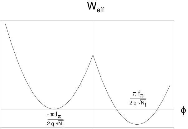
Figure 1: Effective potential at $\theta=0$ for equal chiral phases $\phi=\phi_{u}=\phi_{d}=\phi_{s}$.

The minima are interpreted as two vacua separated by a high potential barrier ($\sim G^{2}$) which is fairly wide, while the energy splitting, $\Delta E$ between the states is fairly small in comparison,

$$\Delta E=m_{q}N_{f}\left|\langle\bar{\Psi}\Psi\rangle\right|\left(1-\cos\frac{2\pi}{qN_{f}}\right)+0(m_{q}^{2}).$$ (13)

Therefore we can use the thin wall approximation [8] in our calculations. The domain wall solution in this approximation corresponding to the effective potential (2) is:

$$\phi_{d.w.}(x) = \frac{pf_{\pi}}{2q\sqrt{N_{f}}}\left[-\frac{\pi}{p}+4\arctan\left\{\tan\left(\frac{\pi}{4p}\right)\exp[\mu(x-x_{0})]\right\}\right]\;\;\;\;\mbox{if }x<x_{0}$$ (14)

$$= \frac{pf_{\pi}}{2q\sqrt{N_{f}}}\left[\frac{\pi}{p}-4\arctan\left\{\tan\left(\frac{\pi}{4p}\right)\exp\left[-\mu(x-x_{0})\right]\right\}\right]\;\;\;\;\mbox{if }x>x_{0}\;,$$

where $x_{0}$ is the position of the center of the domain wall and

$$\mu\equiv\left.\sqrt{\frac{d^{2}W_{eff}}{d\phi^{2}}}\right|_{min}=\frac{2q\sqrt{N_{f}}\sqrt{E}}{pf_{\pi}}$$ (15)

is the inverse width of the wall. The solution (14) is shown as a function of $x-x_{0}$ in Fig. (2).

Figure 2: Domain wall profile.

Its first derivative is continuous at $x=x_{0}$, but the second derivative exhibits a jump. The wall surface tension is given by:

$$\sigma=\frac{4p}{q\sqrt{N_{f}}}f_{\pi}\sqrt{\langle\frac{b\alpha_{s}}{32\pi}G^{2}\rangle}\,\left(1-\cos\frac{\pi}{2p}\right)+0(m_{q}f_{\pi}^{2}).$$ (16)

In what follows we use this domain wall solution in our calculation of the decay rate per unit volume of the false vacuum for both zero and high temperature field theory. The next section describes the semiclassical calculation.

3 Semiclassical Theory

The fate of the false vacuum was discussed in [8] and the expression of $\Gamma/V$ has the form:

$$\Gamma/V=Ae^{-B/\hbar}[1+O(\hbar)].$$ (17)

The semiclassical approximation at zero temperature tells us that B is given by the Euclidean action of $\phi$:

$$B=S_{4}=\int d\tau d^{3}\vec{x}\>\left[\frac{1}{2}(\frac{\partial\phi}{\partial\tau})^{2}+\frac{1}{2}(\nabla\phi)^{2}+U(\phi)\right],$$ (18)

where $U(\phi)$ is the potential, $W_{eff}$, for the chiral phases described in the previous section neglecting the energy difference, $\Delta E$, between the two vacua:

$$U(\phi)=\left\{\begin{array}[]{ll}E\left[1-\cos\left(\frac{2q\sqrt{N_{f}}}{pf_{\pi}}\phi-\frac{\pi}{p}\right)\right]&\mbox{if $\phi\geq 0$ }\\ E\left[1-\cos\left(\frac{2q\sqrt{N_{f}}}{pf_{\pi}}\phi+\frac{\pi}{p}\right)\right]&\mbox{if $\phi\leq 0$. }\end{array}\right.$$ (21)

In order for this to be finite we must have $\lim_{r\rightarrow\infty}\phi(r)=\phi_{-}\equiv\pi f_{\pi}/2q\sqrt{N_{f}}$ where $r=\sqrt{x^{2}+y^{2}+z^{2}+t^{2}}$. The solution of this problem is the four dimensional equivalent to the solution which Coleman calls “the bounce”[8]. It describes a bubble of the true vacuum in the false vacuum at the origin which forms, grows to a maximum size and then shrinks to nothing again (ie. an O(4) invariant bubble). In the thin wall approximation the bounce solution is:

$$\phi_{b}(r)=\left\{\begin{array}[]{l}\phi_{-}\>\>\mbox{for}\>\>r\ll R\\ \phi_{d.w.}(r-R)\>\>\mbox{for}\>\>r\approx R\\ \phi_{+}\>\>\mbox{for}\>\>r\gg R\end{array}\right.,$$

and the value of B is calculated to obtain[8]:

$$\Gamma/V\propto\exp\left(-S_{4}[\phi_{b}]\right)=\exp\left(-\frac{27\pi^{2}\sigma^{4}}{2(\Delta E)^{3}}\right),$$ (22)

where $\sigma$ is the domain wall energy and:

$$S_{4}[\phi_{b}]=\frac{3^{3}\cdot 2^{7}\cdot\pi^{2}p^{4}}{q^{4}N_{f}^{5}}\,\frac{f_{\pi}^{4}E^{2}}{M^{3}}\,\frac{\left(1-\cos\frac{\pi}{2p}\right)^{4}}{\left(1-\cos\frac{2\pi}{qN_{f}}\right)^{3}}\simeq\frac{27}{256}\,\frac{\pi^{4}q^{2}N_{f}}{p^{4}}\,\frac{f_{\pi}^{4}\langle\frac{b\alpha_{s}}{32\pi}G^{2}\rangle^{2}}{m_{q}^{3}\left|\langle\bar{\Psi}\Psi\rangle\right|^{3}}\;$$ (23)

is the Euclidean action of the 4D bounce solution.

The thin wall approximation is valid because the radius of the 4D bubble, which is found to be $R=3\sigma/\Delta E$ by minimizing the value $S_{4}[\phi_{b}]$ , is much larger than the width of the domain wall, $1/\mu$.

For finite temperature QCD the semiclassical approximation is slightly different. At sufficiently high temperature the bubble solution becomes a stable O(3) invariant bubble with radius[23]:

$$R(T)=\frac{2S_{1}(T)}{\Delta E}.$$ (24)

where the temperature dependence of the domain wall energy, $S_{1}(T)$, is not known. In this case the calculation of B gives[23]:

$$\Gamma/V\propto\exp(-S_{3}[\phi_{b}]/T)=\exp\left(-\frac{16\pi S_{1}(T)^{3}}{3(\Delta E)^{2}T}\right).$$ (25)

It should be noted that this decay rate is for the ground state of the metastable well. The decay rate for excited energy states above the metastable vacuum via thermally activated transitions while similar in form is not the same[24].

This completes the semiclassical analysis of the decay rate. In the next section we calculate the quantum corrections to the decay rate in the zero temperature theory.

4 Quantum Corrections at Zero Temperature

The quantum corrections at zero temperature correspond to the coefficient A in Eq.(17)[25]:

$$A=\left|\frac{\det[-\partial_{\mu}\partial^{\mu}+U^{\prime\prime}(\phi_{b})]}{\det[-\partial_{\mu}\partial^{\mu}+U^{\prime\prime}(\phi_{-})]}\right|^{-1/2}.$$ (26)

The spectrum of the operator in the numerator consists of a discrete spectrum with zero and negative eigenvalues and a continuous positive eigenvalue spectrum starting at $\omega^{2}\equiv U^{\prime\prime}(\phi_{-})$. These two parts of the spectrum must be analyzed separately and it can be shown that this factor separates into three parts:

$$A=\left(\omega^{4}\int d^{4}x\left(\frac{B}{2\pi}\right)^{2}\right)\frac{\omega}{\sqrt{\lambda_{-}}}\left|\frac{\det^{\prime}[-\partial_{\mu}\partial^{\mu}+U^{\prime\prime}(\phi_{b})]}{(\omega^{-2})^{5}\det[-\partial_{\mu}\partial^{\mu}+\omega^{2}]}\right|^{-1/2}.$$ (27)

The first term comes from the zero eigenvalues. The second term comes from the negative eigenvalue. The third term is the determinant of the continuous positive eigenvalue spectrum where $\det^{\prime}$ means that the zero and negative eigenvalues are to be omitted. With these eigenvalues omitted the perturbed operator in the numerator has five less eigenvalues in the spectrum because five of the eigenvalues of the unperturbed operator in the denominator have become part of the discrete spectrum of the perturbed operator. Assuming these eigenvalues have originated from the bottom of the unperturbed continuous spectrum we divide through the third term by a factor of $\omega^{2}$ for each omitted eigenvalue. The contributions from the zero and negative eigenvalues are normalized with a factor of $\omega$ keeping each of the three terms dimensionless.

4.1 Positive Eigenvalues

The contribution of the positive eigenvalues requires the evaluation of the determinant ratio:

$$\left|\frac{\det^{\prime}[-\partial_{\mu}\partial^{\mu}+U^{\prime\prime}(\phi_{b})]}{(\omega^{-2})^{5}\det[-\partial_{\mu}\partial^{\mu}+\omega^{2}]}\right|.$$ (28)

However, since the $(\omega^{-2})^{5}$ in the denominator corresponds to a set of measure zero in the continuous eigenvalue spectrum we can omit it and the notation det’ which indicates omission of a discrete set of eigenvalues.

This determinant ratio will turn out to be infinite and to obtain a finite answer we must divide by an infinite factor. The determinant in the numerator can be expanded in the following way:

$$\det|-\partial_{\mu}\partial^{\mu}+U^{\prime\prime}(\phi_{b})|=\exp\left[Tr\log\left\{-\partial_{\mu}\partial^{\mu}+\omega^{2}+V_{pert}(r)\right\}\right]$$ (29)

$$=\det|-\partial_{\mu}\partial^{\mu}+\omega^{2}|\times$$

$$\exp\>Tr\left[\frac{V_{pert}(r)}{-\partial_{\mu}\partial^{\mu}+\omega^{2}}-\frac{1}{2}\left(\frac{V_{pert}(r)}{-\partial_{\mu}\partial^{\mu}+\omega^{2}}\right)^{2}+\frac{1}{3}\left(\frac{V_{pert}(r)}{-\partial_{\mu}\partial^{\mu}+\omega^{2}}\right)^{3}+\cdots\right].$$

It should be noted that the determinant is equal to the partition function of the self interacting massive scalar particle and that the second factor in the last line is expanded up to one loop contributions with three interactions with the effective external potential(see Fig. 3). Tracing over a Cartesian basis we can see that the one and two interaction contributions are divergent but the three interaction contribution is finite:

$$Tr\left[\frac{V_{pert}(r)}{-\partial_{\mu}\partial^{\mu}+\omega^{2}}\right] = \int d^{4}x\;d^{4}k\;\frac{V_{pert}(r)}{k^{2}+\omega^{2}},$$ (30)

$$Tr\left[\left(\frac{V_{pert}(r)}{-\partial_{\mu}\partial^{\mu}+\omega^{2}}\right)^{2}\right] = \int\;d^{4}k\;d^{4}p\;\frac{{\cal V}_{pert}(k)}{(k^{2}+\omega^{2})}\frac{{\cal V}_{pert}(-k)}{((k+p)^{2}+\omega^{2})},$$ (31)

$$Tr\left[\left(\frac{V_{pert}(r)}{-\partial_{\mu}\partial^{\mu}+\omega^{2}}\right)^{3}\right] = \int\;d^{4}k\;d^{4}p\;d^{4}q\;\frac{{\cal V}_{pert}(k)}{(k^{2}+\omega^{2})}\frac{{\cal V}_{pert}(p)}{(p^{2}+\omega^{2})}\frac{{\cal V}_{pert}(-k-p)}{((k+p+q)^{2}+\omega^{2})}.$$ (32)

Figure 3: Expansion of the partition function.

where ${\cal V}_{pert}(k)$ is the Fourier transform of the $V_{pert}(r)$. We will only get a finite answer if we divide through by the infinite factors.

The actual calculation is most easily done using hyperspherical coordinates in four dimensions, $(r,\theta,\phi,\psi)$, and expanding the eigenfunctions $\chi(r,\theta,\phi,\psi)$ in terms of the 4D hyperspherical harmonics:

$$\chi(r,\theta,\phi,\psi)=\sum_{n=0}^{\infty}\sum_{l=-n}^{n}\sum_{m=-|l|}^{|l|}C_{nlm}\frac{u(r)}{r^{3/2}}Y_{nlm}(\theta,\phi,\psi),$$ (33)

which are discussed in the appendix.

In this situation the Laplacian, when operating on each term of (33) with quantum number ‘n’, becomes:

$$\partial_{\mu}\partial^{\mu}\rightarrow\frac{1}{r^{3/2}}\left[\frac{d^{2}}{dr^{2}}-\frac{4n^{2}+8n+3}{4r^{2}}\right]r^{3/2}\equiv\frac{1}{r^{3/2}}{\cal D}_{n}r^{3/2}.$$ (34)

There are 2n(n+2)+1 such terms corresponding to different values of ‘l’ and ‘m’ but with the same eigenvalue. Therefore:

$$\det[-\partial_{\mu}\partial^{\mu}+U^{\prime\prime}]=\prod_{n=0}^{\infty}(\det[-{\cal D}_{n}+U^{\prime\prime}])^{2n(n+2)+1}.$$ (35)

First consider the denominator of (28), $\det[-{\cal D}_{n}+\omega^{2}]$. In order to calculate this determinant we need to solve the eigenvalue equation:

$$[{\cal D}_{n}-\omega^{2}+\lambda]u(r)=0.$$ (36)

The solutions to this differential equation that are well behaved at $r=0$ and $r=\infty$ are:

$$u(r)=(\omega_{\lambda}r)^{3/2}\jmath_{n}(\omega_{\lambda}r)\equiv\sqrt{\frac{\pi\omega_{\lambda}r}{2}}J_{n+1}(\omega_{\lambda}r),$$ (37)

where $\omega_{\lambda}\equiv\sqrt{\lambda-\omega^{2}}$. $\jmath_{n}$ are the 4D analogs of the spherical Bessel functions and $J_{n+1}(x)$ are Bessel functions of the first kind. These solutions become purely oscillatory as $r\rightarrow\infty$. Notice that this solution is only well defined for $\lambda>\omega^{2}$ and indeed there are no solutions for values of $\lambda\leq\omega^{2}$ which are well behaved at $r=0$ and $r=\infty$. Therefore the continuous spectrum of eigenvalues can be written as $\lambda=\omega^{2}+\omega^{2}_{\lambda}$ and:

$$\det[-{\cal D}_{n}+\omega^{2}]=\prod(\omega^{2}+\omega^{2}_{\lambda}).$$ (38)

The numerator of (28) involves the “potential” $U^{\prime\prime}(\phi_{b}(r))$.

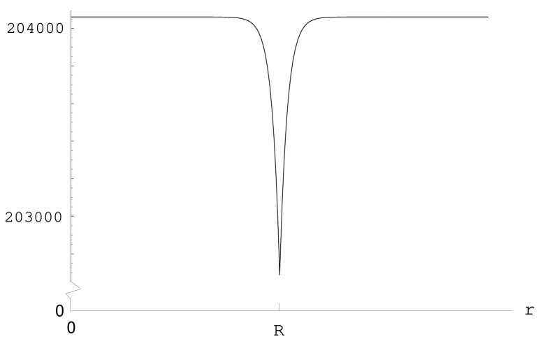
Figure 4: The “potential” $U^{\prime\prime}(\phi_{b}(r))$.

For the symmetrized effective potential (21) the “potential” for this problem is approximately constant except for a small perturbation in a small region near the bubble wall (see Fig.4). The constant potential has been analyzed above. The solutions with or without the perturbations are identical for $r\ll R$ and almost identical for $r\gg R$. The perturbed solution differs from the unperturbed solution in this latter region at most by normalization and a phase shift, $\tilde{\omega}_{\lambda}r=\omega_{\lambda}r+\delta(\omega_{\lambda})$. In this situation, for each value of n, we can obtain the ratio of determinants for a discrete spectrum by [26]:

$$\prod\frac{\omega^{2}+\tilde{\omega}_{\lambda}^{2}}{\omega^{2}+\omega_{\lambda}^{2}}=\exp\left(\sum\ln\frac{\omega^{2}+\tilde{\omega}_{\lambda}^{2}}{\omega^{2}+\omega_{\lambda}^{2}}\right)\approx\exp\left(\sum\frac{2\omega_{\lambda}(\tilde{\omega}_{\lambda}-\omega_{\lambda})}{\omega^{2}+\omega_{\lambda}^{2}}\right),$$ (39)

which becomes in the continuum:

$$\exp\left[\frac{1}{\pi}\int_{0}^{\infty}d\omega_{\lambda}\frac{2\omega_{\lambda}\delta(\omega_{\lambda})}{\omega^{2}+\omega_{\lambda}^{2}}\right].$$ (40)

This formula gives the determinant ratio for a particular value of ‘n’ if we know the phase shifts, $\delta(\omega_{\lambda})$. In order to calculate the phase shifts, however, we must make further approximations.

Consider both the perturbed and the unperturbed equations:

$$\left[\frac{d^{2}}{dr^{2}}-\frac{4n^{2}+8n+3}{4r^{2}}+(\lambda-\omega^{2})\right]u(r)=0,$$ (41)

$$\left[\frac{d^{2}}{dr^{2}}-\frac{4n^{2}+8n+3}{4r^{2}}+\left(\lambda-\omega^{2}+V_{\mbox{pert}}(r)\right)\right]v(r)=0.$$ (42)

Multiply (41) by $v(r)$ and (42) by $u(r)$, subtract, and integrate from 0 to $\infty$ to obtain:

$$\int_{0}^{\infty}\left(u^{\prime\prime}(r)v(r)-v^{\prime\prime}(r)u(r)\right)dr=\left(u^{\prime}(r)v(r)-v^{\prime}(r)u(r)\right)|_{0}^{\infty}=\int_{0}^{\infty}V_{\mbox{pert}}(r)u(r)v(r)dr.$$ (43)

Using the fact that both solutions vanish at $r=0$ and using the asymptotic form of the Bessel functions we obtain an exact formula for the phase shift, $\delta(\omega_{\lambda})$:

$$\sin\delta(\omega_{\lambda})=\frac{1}{\omega_{\lambda}}\int_{0}^{\infty}V_{\mbox{pert}}(r)u(r)v(r)dr.$$ (44)

Of course, since the perturbed differential equation is extremely difficult to solve, we use perturbation theory to obtain:

$$\delta(\omega_{\lambda})\approx\delta(\omega_{\lambda})_{0}=\frac{1}{\omega_{\lambda}}\int_{0}^{\infty}V_{\mbox{pert}}(r)u(r)^{2}dr=\frac{\pi}{2}\int_{0}^{\infty}V_{\mbox{pert}}(r)rJ_{n+1}(\omega_{\lambda}r)^{2}dr,$$ (45)

for small phase shifts. Using this result for the phase shift in Equation (40), we obtain the ratio of determinants:

$$\left|\frac{-\det[{\cal D}_{n}+U^{\prime\prime}(\phi_{b})]}{\det[-{\cal D}_{n}+\omega^{2}]}\right|\approx\exp\left[\int_{0}^{\infty}\int_{0}^{\infty}d\omega_{\lambda}dr\frac{\omega_{\lambda}r}{\omega^{2}+\omega_{\lambda}^{2}}V_{\mbox{pert}}(r)J_{n+1}(\omega_{\lambda}r)^{2}\right].$$ (46)

for each value of n.

Figure 5: The perturbation $V_{pert}(r)$ is the dotted line and the approximate perturbation $\tilde{V}_{pert}(r)$ is the solid line.

The complete determinant ratio then becomes:

$$\left|\frac{\det[-\partial_{\mu}\partial^{\mu}+U^{\prime\prime}(\phi_{b})]}{\det[-\partial_{\mu}\partial^{\mu}+\omega^{2}]}\right|=\exp\sum_{n=0}^{\infty}(2n(n+2)+1)\left[\int_{0}^{\infty}\int_{0}^{\infty}d\omega_{\lambda}dr\frac{\omega_{\lambda}r}{\omega^{2}+\omega_{\lambda}^{2}}V_{\mbox{pert}}(r)J_{n+1}(\omega_{\lambda}r)^{2}\right].$$ (47)

for an arbitrary perturbation potential. The next step in our analysis is to take into account the specific potential in our problem.

It should be noted that this approximation gives the same result as the exact answer expanded to one loop (see Eq.29 and 30) where the trace is taken instead over $|rnlm\rangle$, $|knlm\rangle$ bases.

This formula is suitable for numerical evaluation, but in order to obtain an analytical answer we must approximate the perturbation in the potential $U^{\prime\prime}$ by:

$$\tilde{V}_{\mbox{pert}}(r)=\left\{\begin{array}[]{l}-\beta\frac{10(r-\frac{11R}{10})^{2}}{R^{2}}~{}~{}R>r>\frac{11R}{10}\\ -\beta\frac{10(r-\frac{9R}{10})^{2}}{R^{2}}~{}~{}\frac{9R}{10}>r>R\\ ~{}~{}~{}~{}~{}~{}~{}0~{}~{}~{}~{}~{}~{}~{}~{}~{}~{}~{}\mbox{otherwise}\end{array},\right.$$ (48)

where $\beta=\left(U^{\prime\prime}(\phi(0))-U^{\prime\prime}(\phi(R))\right)$(see Fig. 5). With this approximate potential we find the phase shift via (45):

$$\delta_{0}(\omega_{\lambda})=-200\frac{\beta}{R^{2}}\left[{\frac{121}{200}r^{2}R^{2}\left(J_{n+1}(r\omega_{\lambda})^{2}-J_{n}(r\omega_{\lambda})J_{n+2}(r\omega_{\lambda})\right)}\right.~{}~{}~{}~{}~{}~{}~{}~{}~{}~{}~{}~{}~{}~{}~{}~{}~{}~{}~{}~{}~{}~{}~{}~{}~{}~{}~{}~{}~{}~{}~{}~{}~{}~{}~{}~{}~{}$$

$$+\frac{2^{-4-2n}r^{4}(r\omega_{\lambda})^{2+2n}}{(n+4)!(n+1)!}\left\{2(n+2)(n+4)\;{}_{1}F_{2}\left(n+\frac{3}{2},n+4,2n+3;-r^{2}\omega_{\lambda}^{2}\right)\right.$$

$$\left.-r^{2}\omega_{\lambda}^{2}\;{}_{1}F_{2}\left(n+\frac{5}{2},n+5,2n+4;-r^{2}\omega_{\lambda}^{2}\right)\right\}$$

$$\left.\frac{11}{10}\frac{2^{-2-2n}r^{3}R(r\omega_{\lambda})^{2+2n}}{(n+\frac{5}{2})[(n+1)!]^{2}}\;{}_{2}F_{3}\left(n+\frac{3}{2},n+\frac{5}{2},n+2,n+\frac{7}{2},2n+3;-r^{2}\omega_{\lambda}^{2}\right)\right]^{11/10R}_{R}.$$ (49)

Figure 6: The phase shift $\delta_{0}(\omega_{\lambda})$ shown as a function of $\omega_{\lambda}$ for various values of n. Notice the changing vertical scale.

Using this result we can verify that $\delta(\omega_{\lambda})\ll 1$ which means that the approximations of (45) are justified. The phase shift as a function of $\omega_{\lambda}$ is shown for a few values of n in Fig.(6). However, (49) is very difficult to work with so we make another approximation. For $\omega_{\lambda}$ large enough we can use the asymptotic approximation for the Bessel function in (45),

$$J_{n+1}(x)=\sqrt{\frac{2}{\pi x}}\left\{P_{n+1}(x)\cos\left[x-\left(n+\frac{3}{2}\right)\frac{\pi}{2}\right]-Q_{n+1}(x)\sin\left[x-\left(n+\frac{3}{2}\right)\frac{\pi}{2}\right]\right\},$$ (50)

where:

$$P_{n+1}(x) = 1-\frac{(\mu-1)(\mu-9)}{2!\;(8x)^{2}}+\frac{(\mu-1)(\mu-9)(\mu-25)(\mu-49)}{4!\;(8x)^{4}}-\cdots,$$ (51)

$$Q_{n+1}(x) = \frac{(\mu-1)}{1!\;(8x)}-\frac{(\mu-1)(\mu-9)(\mu-25)}{3!\;(8x)^{3}}+\cdots,$$ (52)

$$\mu = 4(n+1)^{2}.$$ (53)

In this way we find:

$$\delta_{0}(\omega_{\lambda}) \approx \frac{2R\beta}{30\pi\omega_{\lambda}}+\frac{(-1)^{n}\beta}{\pi}\frac{\cos(2R\omega_{\lambda})}{\omega_{\lambda}^{2}}+{\cal O}(1/\omega_{\lambda}^{3}).$$ (54)

Of course this estimate for $\delta_{0}(\omega_{\lambda})$ has an infrared cutoff in $\omega_{\lambda}$ below which it is not a good estimate and this will be true no matter how many terms in the approximation of the Bessel function we keep. Therefore as a first approximation we keep only the first term and cut off the $\omega_{\lambda}$ integral at the position of the first peak in $\delta_{0}(\omega_{\lambda})$. Using this approximation for $\delta_{0}(\omega_{\lambda})$ we obtain our first estimate of the ratio of determinants for each value of the quantum number ’n’ given by:

$$\frac{\det[-{\cal D}_{n}+U^{\prime\prime}(\phi_{b})]}{\det[-{\cal D}_{n}+U^{\prime\prime}(\phi_{-})]}\approx\exp\left[\frac{2R\beta}{30\pi\omega}\arctan\left(\frac{\omega}{\bar{\omega}(n)}\right)\right],$$ (55)

where $\bar{\omega}(n)\approx 33.16n+72=an+b$ is the infrared cutoff given by the location of the first peak in $\delta_{0}(\omega_{\lambda})$. Using the result (55) we can calculate our first approximation for the complete determinant ratio. For large values of n the terms of the sum in (47) approach:

$$\frac{4R\beta}{30\pi\omega}n^{2}\left(\frac{\omega}{an}\right),$$ (56)

and therefore the sum is infinite. Our first estimate for the complete determinant ratio based on (47) is infinite. This was to be expected based on comments at the beginning of this section and, since this approximation exactly coincides with the tadpole diagram, we subtract this term from the exponent as our normalization prescription for the complete determinant ratio. Note that we have used the approximation of (54) to calculate the infinite factor but the equality with the tadpole diagram holds before this approximation was made.

In order to find a finite result we must adjust our earlier approximation for the phase shift:

$$\delta(\omega_{\lambda})=\arcsin(\delta_{0}(\omega_{\lambda}))=\delta_{0}(\omega_{\lambda})+\frac{1}{6}\delta_{0}(\omega_{\lambda})^{3}+\frac{3}{40}\delta_{0}(\omega_{\lambda})^{5}+\cdots$$ (57)

which would add correction terms to the exponent in (55). The second term in (57) leads to a factor of the form:

$$\exp\left[\frac{\pi^{2}}{24}\int_{0}^{\infty}d\omega_{\lambda}\frac{\omega_{\lambda}\delta_{0}(\omega_{\lambda})^{3}}{\omega^{2}+\omega_{\lambda}^{2}}\right],$$ (58)

for each value of n. This term is also divergent but does not exactly coincide with the next term in the expansion (29). However, the divergent contribution in each must be the same.

Therefore dividing through by the previously obtained infinite factor (ie. the right hand side of (55)) leads to the renormalized value:

$$\frac{\det[-{\cal D}_{n}+U^{\prime\prime}(\phi_{b})]}{\det[-{\cal D}_{n}+U^{\prime\prime}(\phi_{-})]}\approx\exp\left[\frac{\pi^{2}}{24}\left(\frac{2R\beta}{30\pi\omega}\right)^{3}\left\{\frac{\omega}{\bar{\omega}(n)}-\arctan\left(\frac{\omega}{\bar{\omega}(n)}\right)\right\}\right],$$ (59)

For large values of $n$ the terms of the sum in (47) approach:

$$\frac{\pi^{2}}{24}\left(\frac{2R\beta}{30\pi\omega}\right)^{3}(2n^{2}+4n+1)\left(\frac{\omega^{3}}{3a^{3}n^{3}}\right).$$ (60)

which also leads to a divergent sum and therefore an infinite value for the determinant ratio. The divergence here must be contained in the divergence in the two interaction term of the expansion (29), as are other logarithmic divergences obtained from keeping more terms in the approximation of the Bessel function (50). However, subtracting the two interaction term will almost certainly leave a finite contribution at the next order in $n$. We will assume this is the case but since we are doing an approximate calculation we will not calculate the finite contribution from the two interaction term or any correction terms to our approximation since they will have the same physical dependence as the approximation we will give. We should further note that correction terms are probably not calculable analytically and are not likely to be a problem for our results. They are obtained from integrating oscillatory functions (see second term in (54)) over $\omega_{\lambda}$ in (58) and should not contribute very much. The renormalized approximation to the complete determinant ratio (47) that we obtain from (59) is given by:

$$\exp\frac{\pi^{2}}{24}\left(\frac{2R\beta}{30\pi\omega}\right)^{3}\left[\sum_{n=0}^{\infty}(2n(n+2)+1)\left\{\frac{\omega}{\bar{\omega}(n)}-\arctan\left(\frac{\omega}{\bar{\omega}(n)}\right)\right\}-\sum_{n=1}^{\infty}2n^{2}\frac{\omega^{3}}{3a^{3}n^{3}}\right]$$ (61)

$$=\exp\frac{\pi^{2}}{24}\left(\frac{2R\beta}{30\pi\omega}\right)^{3}\left[\sum_{n=0}^{100}(2n(n+2)+1)\left\{\frac{\omega}{\bar{\omega}(n)}-\arctan\left(\frac{\omega}{\bar{\omega}(n)}\right)\right\}\right.$$

$$\left.-\sum_{n=1}^{100}\left\{(2n(n+2)+1)\frac{\omega^{3}}{3a^{3}n^{3}}\right\}+\frac{4\omega^{3}}{3a^{3}}\zeta(2)+\frac{\omega^{3}}{3a^{3}}\zeta(3)\right].$$ (62)

Evaluating gives:

$$\exp\left[-5300\frac{\pi^{2}}{24}\left(\frac{2R\beta}{30\pi\omega}\right)^{3}\right]\approx\exp[-2\times 10^{-5}].$$ (63)

Because of the small value of the exponent we can see that the exponential is extremely well approximated by:

$$\exp\left[\frac{-5300\pi^{2}}{24}\left(\frac{2R\beta}{30\pi\omega}\right)^{3}\right]\approx 1-\frac{5300\pi^{2}}{24}\left(\frac{2R\beta}{30\pi\omega}\right)^{3}.$$ (64)

which is our result for the determinant ratio (28).

This is a nonperturbative calculation because Eq.(40) is a nonperturbative resummation of the perturbation expansion (29) of the determinant. While we make an approximation through Eq.(57) this expansion is nonperturbative since the terms of the expansions do not coincide. Our approximate calculation should therefore have contributions from all perturbative diagrams. This nonperturbative resummation of diagrams in the determinantal prefactor is very similar in spirit to that of [27].

This result constitutes the contribution of the positive eigenvalues to the quantum corrections to the decay rate in the zero temperature theory. In the next section we consider the zero and negative eigenvalues.

4.2 Zero and Negative Eigenvalues

The zero eigenvalues contribute $\sqrt{B/2\pi}$ per collective coordinate[8]. The action of the 4D bubble is independent of the center of the bubble which means there are 4 collective coordinates leading to the first factor in Eq.(27).

The eigenfunctions of zero eigenvalue are:

$$\chi_{o\mu}(x,y,z,t)=\frac{d}{dx^{\mu}}\phi_{b}(r)=\frac{dr}{dx^{\mu}}\;\frac{d}{dr}\phi_{b}(r)=\frac{x^{\mu}}{r}\;\frac{d}{dr}\phi_{b}(r),$$ (65)

where $r=\sqrt{x^{2}+y^{2}+z^{2}+t^{2}}$ and:

$$t= r\;Cos(\psi) \sim Y_{100},$$ (66)

$$z= r\;Cos(\theta)Sin(\psi) \sim Y_{110},$$ (67)

$$y= r\;Cos(\phi)Sin(\theta)Sin(\psi) \sim Y_{111}+Y_{11-1},$$ (68)

$$y= r\;Sin(\phi)Sin(\theta)Sin(\psi) \sim Y_{111}-Y_{11-1}.$$ (69)

Therefore these eigenfunctions all correspond to $n=1$ and since there are no radial nodes we can be sure that there are no negative eigenvalues with $n\neq 0$.

In [28], Coleman argued that there is only a single negative eigenvalue for an O(4) invariant bounce. We assume this and determine its value. We use the method of [8] with a slight modification. As was argued by Coleman, the only possible eigenfunctions of negative eigenvalue are those that are bound to the bubble wall. For such eigenfunctions we can approximate the centrifugal potential in (34) by a constant determined by its value at the bubble wall ($r=R$):

$$\lambda_{pn}=\lambda_{p}+\frac{4n^{2}+8n+3}{4R^{2}},$$ (70)

where $\lambda_{p}$ is a number independent of $n$. We know that for $n=1$ the lowest eigenvalue is zero:

$$\lambda_{01}=\lambda_{0}+\frac{15}{4R^{2}}=0.$$ (71)

Therefore we can obtain the lowest eigenvalue for $n=0$:

$$\lambda_{-}=\lambda_{00}=\lambda_{0}+\frac{3}{4R^{2}}=-\frac{15}{4R^{2}}+\frac{3}{4R^{2}}=-\frac{3}{R^{2}}.$$ (72)

This value is different from Coleman’s but only by a factor of 2. We cannot explain this discrepancy but can only stand by our calculation.

4.3 Decay Rate for Zero Temperature

Therefore combining the zero temperature semiclassical result (22) with the quantum corrections obtained in the last section we estimate the decay rate per unit volume of the false vacuum in the zero temperature theory to be:

$$\Gamma/V = \exp\left(-S_{4}\right)\left(\omega^{4}\left(\frac{S_{4}}{2\pi}\right)^{2}\right)\frac{\omega}{\sqrt{\lambda_{-}}}\left|\frac{\det^{\prime}[-\partial_{\mu}\partial^{\mu}+U^{\prime\prime}(\phi_{b})]}{(\omega^{-2})^{5}\det[-\partial_{\mu}\partial^{\mu}+\omega^{2}]}\right|$$ (73)

$$= \exp\left(-\frac{27\pi^{2}\sigma^{4}}{2(\Delta E)^{3}}\right)\left(\frac{27\pi^{2}\sigma^{4}\omega^{2}}{4\pi(\Delta E)^{3}}\right)^{2}\frac{R\omega}{\sqrt{3}}\left[1-\frac{5300\pi^{2}}{24}\left(\frac{2R\beta}{30\pi\omega}\right)^{3}\right]^{-1/2}$$ (74)

$$= 1.55\times 10^{-18}\mbox{MeV}^{4}\approx 3\times 10^{-4}\mbox{fm}^{-3}\mbox{s}^{-1}.$$ (75)

It should be noted that the quantum corrections are negligible so the decay rate is basically determined by the semiclassical result. We believe that this observation would be unchanged by the inclusion of corrections that we have ignored in this calculation. While the quantum corrections did not turn out be significant in this case, the fact that they are not is relevant to the baryogenesis mechanism described in [7]. As well, the techniques applied to the problem may prove useful in other calculations of this type.

In the next section we perform the same calculation in the high temperature limit.

5 Quantum Corrections for High Temperature

The quantum corrections to the decay rate at high temperature correspond to[23]:

$$A=T\left(\omega^{3}\int d^{3}x\left(\frac{S_{3}[\phi_{b}]}{2\pi T}\right)^{3/2}\right)\frac{\omega}{\sqrt{\lambda_{-}}}\left|\frac{\det^{\prime}[-\partial_{i}\partial^{i}+U^{\prime\prime}(\phi_{b})]}{(\omega^{-2})^{3}\det[-\partial_{i}\partial^{i}+U^{\prime\prime}(\phi_{-})]}\right|^{-1/2}.$$ (76)

which again factors into three parts corresponding to zero, negative and positive eigenvalues respectively.

5.1 Positive Eigenvalues

The calculation in three dimensions is extremely similar to the four dimensional calculation presented in the Sect. 4. The expansion of the determinant ratio is exactly the same as in 4D (29). Tracing over Cartesian bases we can see that the one loop term is divergent while the two loop term is finite:

$$Tr\left[\frac{V_{pert}(r)}{-\partial_{\mu}\partial^{\mu}+\omega^{2}}\right] = \int d^{3}x\;d^{3}k\;\frac{V_{pert}(r)}{k^{2}+\omega^{2}},$$ (77)

$$Tr\left[\left(\frac{V_{pert}(r)}{-\partial_{\mu}\partial^{\mu}+\omega^{2}}\right)^{2}\right] = \int\;d^{3}k\;d^{3}p\;\frac{{\cal V}_{pert}(k)}{(k^{2}+\omega^{2})}\frac{{\cal V}_{pert}(-k)}{((k+p)^{2}+\omega^{2})}.$$ (78)

The calculation is done using spherical coordinates and the eigenfunctions are expanded in terms of the spherical harmonics:

$$\chi(r,\theta,\phi)=\sum_{n=0}^{\infty}\sum_{l=-n}^{n}\sum_{m=-|l|}^{|l|}C_{lm}\frac{u(r)}{r}Y_{lm}(\theta,\phi).$$ (79)

For each value of $l$ the Laplacian becomes:

$$\partial_{i}\partial^{i}\rightarrow\frac{1}{r}\left[\frac{d^{2}}{dr^{2}}-\frac{l(l+1)}{r^{2}}\right]r\equiv\frac{1}{r}{\cal D}_{l}r.$$ (80)

Therefore:

$$\det[-\partial_{i}\partial^{i}+U^{\prime\prime}]=\prod_{l=0}^{\infty}(\det[-{\cal D}_{l}+U^{\prime\prime}])^{2l+1}.$$ (81)

The solutions to this differential equation that are well behaved at $r=0$ and $r=\infty$ are:

$$u(r)=\omega_{\lambda}rj_{l}(\omega_{\lambda}r)\equiv\sqrt{\frac{\pi\omega_{\lambda}r}{2}}J_{l+1/2}(\omega_{\lambda}r),$$ (82)

where $j_{l}$ are the usual spherical Bessel functions and $\omega_{\lambda}\equiv\sqrt{\lambda-\omega^{2}}$. We obtain:

$$\delta(\omega_{\lambda})\approx\frac{1}{\omega_{\lambda}}\int_{0}^{\infty}V_{\mbox{pert}}(r)u(r)^{2}dr=\frac{\pi}{2}\int_{0}^{\infty}V_{\mbox{pert}}(r)rJ_{l+1/2}(\omega_{\lambda}r)^{2}dr,$$ (83)

thus giving :

$$\left|\frac{\det[-\partial_{i}\partial^{i}+U^{\prime\prime}(\phi_{b})]}{\det[-\partial_{i}\partial^{i}+\omega^{2}]}\right|=\exp\sum_{l=0}^{\infty}(2l+1)\left[\int_{0}^{\infty}\int_{0}^{\infty}d\omega_{\lambda}dr\frac{\omega_{\lambda}r}{\omega^{2}+\omega_{\lambda}^{2}}V_{\mbox{pert}}(r)J_{l+1/2}(\omega_{\lambda}r)^{2}\right].$$ (84)

As in the zero temperature case we can find the exact expression for the phase shift with the approximate potential but it is too difficult to work with. Instead we approximate the Bessel functions as in (50) where $(n+1)\rightarrow(l+1/2)$. In this way we find:

$$\delta(\omega_{\lambda}) \approx \delta_{0}(\omega_{\lambda})=\frac{2R\beta}{30\pi\omega_{\lambda}}+{\cal O}(1/\omega_{\lambda}^{2}).$$ (85)

Our first estimate of the ratio of determinants for each value of the quantum number ’l’ is given by:

$$\frac{\det[-{\cal D}_{l}+U^{\prime\prime}(\phi_{b})]}{\det[-{\cal D}_{l}+U^{\prime\prime}(\phi_{-})]}\approx\exp\left[\frac{2R\beta}{30\pi\omega}\arctan\left(\frac{\omega}{\bar{\omega}(n)}\right)\right],$$ (86)

where $\bar{\omega}(l)\approx 49.5l+82=cl+d$ is the infrared cutoff given by the location of the first peak in $\delta_{0}(\omega_{\lambda})$ as a function of $\omega_{\lambda}$. For large values of $l$ the terms of the sum in (84) approach:

$$\frac{4R\beta}{30\pi\omega}l\left(\frac{\omega}{cl}\right),$$ (87)

and the sum is infinite and therefore the complete determinant ratio is also infinite. Again this was to be expected and, since this approximation exactly coincides with the one loop term, our renormalization prescription is to remove the one loop term from the exponent of (84).

Again we must adjust our earlier approximation for the phase shift:

$$\delta(\omega_{\lambda})=\arcsin(\delta_{0}(\omega_{\lambda}))=\delta_{0}(\omega_{\lambda})+\frac{1}{6}\delta_{0}(\omega_{\lambda})^{3}+\frac{3}{40}\delta_{0}(\omega_{\lambda})^{5}+\cdots$$ (88)

and the correction is implemented as in (58). Evaluating the contribution to the determinant ratio leads to:

$$\frac{\det[-{\cal D}_{l}+U^{\prime\prime}(\phi_{b})]}{\det[-{\cal D}_{l}+U^{\prime\prime}(\phi_{-})]}\approx\exp\left[\frac{\pi^{2}}{24}\left(\frac{2R\beta}{30\pi\omega}\right)^{3}\left\{\frac{\omega}{\bar{\omega}(l)}-\arctan\left(\frac{\omega}{\bar{\omega}(l)}\right)\right\}\right].$$ (89)

For large values of $l$ the terms of the sum in (84) approach:

$$\frac{\pi^{2}}{24}\left(\frac{2R\beta}{30\pi\omega}\right)^{3}(2l+1)\left(\frac{\omega^{3}}{3c^{3}l^{3}}\right).$$ (90)

The sum is finite so we do not need to further normalize and our result for the complete determinant ratio (84) is:

$$\exp\frac{\pi^{2}}{24}\left(\frac{2R\beta}{30\pi\omega}\right)^{3}\left[\sum_{l=0}^{100}(2l+1)\left\{\frac{\omega}{\bar{\omega}(l)}-\arctan\left(\frac{\omega}{\bar{\omega}(l)}\right)\right\}\right.$$

$$\left.-\sum_{l=1}^{100}\left\{(2l+1)\frac{\omega^{3}}{3c^{3}l^{3}}\right\}+\frac{2\omega^{3}}{3a^{3}}\zeta(2)+\frac{\omega^{3}}{3a^{3}}\zeta(3)\right].$$ (91)

Evaluating gives:

$$\exp\left[82\frac{\pi^{2}}{24}\left(\frac{2R\beta}{30\pi\omega}\right)^{3}\right]\approx\exp[3\times 10^{-7}].$$ (92)

Because of the small value of the exponent we can see that the exponential is extremely well approximated by:

$$\exp\left[\frac{82\pi^{2}}{24}\left(\frac{2R\beta}{30\pi\omega}\right)^{3}\right]\approx 1+\frac{82\pi^{2}}{24}\left(\frac{2R\beta}{30\pi\omega}\right)^{3}.$$ (93)

This result constitutes the contribution of the positive eigenvalues to the quantum corrections to the decay rate in the high temperature theory. In the next section we consider the zero and negative eigenvalues.

5.2 Zero and Negative Eigenvalues

In the O(3) invariant bubble there are 3 collective coordinates leading to the first term in (76). The eigenfunctions of zero eigenvalue are:

$$\chi_{o\mu}(x,y,z)=\frac{d}{dx^{\mu}}\phi_{b}(r)=\frac{dr}{dx^{\mu}}\;\frac{d}{dr}\phi_{b}(r)=\frac{x^{\mu}}{r}\;\frac{d}{dr}\phi_{b}(r),$$ (94)

where $r=\sqrt{x^{2}+y^{2}+z^{2}}$ and:

$$z= r\;Cos(\theta) \sim Y_{10},$$ (95)

$$y= r\;Cos(\phi)Sin(\theta) \sim Y_{11}+Y_{1-1},$$ (96)

$$y= r\;Sin(\phi)Sin(\theta) \sim Y_{11}-Y_{1-1}.$$ (97)

Therefore these eigenfunctions all correspond to $l=1$ and since there are no radial nodes we can be sure that there are no negative eigenvalues with $l\neq 0$.

We will assume, as we did in the previous section, that there is only a single negative eigenvalue and concentrate on obtaining an approximation. The only possible eigenfunctions of negative eigenvalue are those that are bound to the bubble wall. For such eigenfunctions we can approximate the centrifugal potential in (80) by a constant:

$$\lambda_{pn}=\lambda_{p}+\frac{l(l+1)}{R^{2}},$$ (98)

where $\lambda_{p}$ is a number independent of $l$. We know that for $l=1$ the lowest eigenvalue is zero:

$$\lambda_{01}=\lambda_{0}+\frac{2}{R^{2}}=0.$$ (99)

Therefore we can obtain the lowest eigenvalue for $l=0$:

$$\lambda_{-}=\lambda_{00}=\lambda_{0}=-\frac{2}{R^{2}}.$$ (100)

5.3 Decay Rate for High Temperature

Therefore combining the high temperature semiclassical result (25) with the quantum corrections obtained in the last section we estimate the decay rate per unit volume of the false vacuum in the high temperature theory to be:

$$\Gamma/V=\frac{R\omega}{\sqrt{2}}\left(\omega^{3}\left(\frac{16\pi S_{1}(T)^{3}}{3(\Delta E)^{2}T}\right)^{3/2}\right)\exp\left(-\frac{16\pi S_{1}(T)^{3}}{3(\Delta E)^{2}T}\right)\left[1+\frac{82\pi^{2}}{24}\left(\frac{2R\beta}{30\pi\omega}\right)^{3}\right]^{-1/2}.$$ (101)

We cannot obtain a numerical estimate for the decay rate at this time since the temperature dependence of the semiclassical result is not currently known. This result could be important to the study of false vacuum states of this type in heavy ion collisions.

6 Conclusion

We have obtained an estimate for the decay rate per unit volume of $\Gamma/V\approx 3\times 10^{-4}\mbox{fm}^{-3}\mbox{s}^{-1}$ for a false vacuum in an effective Lagrangian approach to QCD for zero temperature theory. We have obtained an expression (101) for the decay rate per unit volume in the high temperature theory, which is the best we can do without knowledge of the temperature dependence of the effective potential. These are nonperturbative calculations in that they contain contributions from all orders of perturbation theory.

The value of the decay rate for zero temperature shows that if the universe had started out in a false vacuum state then it would have decayed long ago into the true vacuum state. This is not new or interesting. The interesting thing concerns the possibility that these vacuum bubbles would have significant effects on the evolution of the early universe at around the time of the QCD phase transition.

One such effect related to baryogenesis was described in [7]. The first approximation to the decay rate we have calculated shows that bubbles of false vacuum are far too unstable for this simplified baryogenesis mechanism. The effect of fermions or intrinsic heavy degrees of freedom could go a long way to stabilizing the bubbles because they would make the barrier separating the false vacuum from the true vacuum much higher, thus increasing the stability of the false vacuum. The precise calculation is outside the scope of the present work and we can only say that, so far, this mechanism for baryogenesis at the QCD scale has not been proved viable.

The result does not, however, rule out the possibility of nontrivial effects on the evolution of the early universe. As well, the techniques developed may be useful in the study of arbitrary metastable vacua which seem to be a general feature of gauge theories in the strong coupling regime.

The high temperature expression for the decay rate will be relevant to the possibility of observing CP odd bubbles at RHIC through signatures as described in [14]. As was mentioned previously the false vacuum described in [14] assumed the large $N_{c}$ limit. However, the same effects would manifest themselves in our case which arises from an effective potential valid for arbitrary $N_{c}$

In the future it might be useful to verify numerically our contention that the corrections neglected in the approximation and finite contributions from the renormalization prescription do not significantly alter the results. As well, one could do numerical calculations using the exact numerical domain wall solution in the case of non-degenerate vacuum states. It is possible that the determinant could also be estimated numerically in the non-degenerate case.

It would also be interesting to repeat this calculation using the methods of [16] [17] [18] [19] and compare with the present results.

Appendix A Hyperspherical Harmonics in Four Dimensions

Hyperspherical coordinates in 4D dimensions are related to the Cartesian coordinates by:

$$x=r\;Sin[\psi]Sin[\theta]Sin[\phi],$$ (102)

$$y=r\;Sin[\psi]Sin[\theta]Cos[\phi],$$ (103)

$$z=r\;Sin[\psi]Cos[\theta],$$ (104)

$$w=r\;Cos[\psi].$$ (105)

The Laplacian in 4D in hyperspherical coordinates is:

$$\frac{1}{r^{3}}\partial_{r}\left(r^{3}\partial_{r}\right)+\frac{1}{r^{2}\sin^{2}\psi}\partial_{\psi}\left(\sin^{2}\psi\partial_{\psi}\right)+\frac{1}{r^{2}\sin^{2}\psi\sin\theta}\partial_{\theta}\left(\sin\theta\partial_{\theta}\right)+\frac{1}{r^{2}\sin^{2}\psi\sin^{2}\theta}\partial^{2}_{\phi}.$$ (106)

Assuming separable solutions and treating $\theta$ and $\phi$ coordinates in exactly the same way as in three dimensions we obtain the differential equation:

$$\Psi^{\prime\prime}(\psi)+2\cot(\psi)\Psi^{\prime}(\psi)-l(l+1)\csc^{2}(\psi)\Psi(\psi)=\Lambda\Psi(\psi).$$ (107)

With the substitution $u=Cos[\psi]$ this becomes:

$$(1-u^{2})U^{\prime\prime}(u)-3uU^{\prime}(u)-\frac{l(l+1)}{1-u^{2}}U(u)=BU(u).$$ (108)

If $B=n(n+2)$ and $l(l+1)=l^{\prime}(l^{\prime}+1)$ this can be identified as the differential equation satisfied by the associated type II Chebyshev functions. These can be obtained from the type II Chebyshev differential equation in exactly the same way as associated Legendre functions are obtained from the Legendre differential equation.

As an aside notice that the type II Chebyshev equation is a special case of the Geigenbauer (Ultraspherical) equation:

$$(1-x^{2})\frac{d^{2}}{dx^{2}}C_{n}^{(\alpha)}(x)-(2\alpha+1)x\frac{d}{dx}C_{n}^{(\alpha)}(x)-n(n+2\alpha)C_{n}^{(\alpha)}(x)=0,$$ (109)

with $\alpha=1$. The Legendre polynomial equation corresponds to $\alpha=1/2$. All other hyperspherical coordinates will lead to associated Geigenbauer equations with integer or half integer $\alpha$.

The hyperspherical harmonics in four dimensions are given by:

$$Y_{nlm}(\theta,\phi,\psi)=A(n,l,m)\left\{\begin{array}[]{l}Y_{lm}(\theta,\phi)\;\;U_{n}{}^{l}(\cos(\psi))~{}~{}~{}~{}~{}~{}~{}~{}~{}0\leq l\leq n\\ Y_{|l|m}(\theta,\phi)\;\;U_{n}{}^{l-1}(\cos(\psi))~{}~{}~{}-n\leq l\leq-1\end{array}.\right.$$ (110)

where $Y_{lm}(\theta,\phi)$ are the usual 3D spherical harmonics and $U_{n}{}^{l}$ are associated Chebyshev type II functions defined by:

$$U_{n}{}^{l}(x) = (1-x^{2})^{l/2}\frac{d^{l}}{dx^{l}}U_{n}(x)$$ (111)

$$= (1-x^{2})^{l/2}\frac{(-1)^{n}(n+1)\sqrt{\pi}}{2^{n+1}(n+1/2)!}\frac{d^{l}}{dx^{l}}\left[(1-x^{2})^{-1/2}\frac{d^{n}}{dx^{n}}\left\{(1-x^{2})^{n+1/2}\right\}\right],$$

for $l\geq 0$ and by:

$$U_{n}{}^{l}(x)=\frac{(-1)^{n}(n+1)\sqrt{\pi}}{2^{n+1}(n+1/2)!}(1-x^{2})^{l/2}\frac{d^{n+l+1}}{dx^{n+l+1}}\left[(1-x^{2})^{n+1/2}\right],$$ (112)

for $l\leq-2$. These hyperspherical harmonics form a complete orthogonal basis for the functions of the angular variables in four dimensions.

$$\sum_{n=0}^{\infty}\sum_{l=-n}^{n}\sum_{m=-l}^{l}Y^{*}_{nlm}(r,\theta,\phi,\psi)Y_{nlm}(r^{\prime},\theta^{\prime},\phi^{\prime},\psi^{\prime})=\frac{\delta(\psi-\psi^{\prime})}{\sin^{2}\psi}\frac{\delta(\theta-\theta^{\prime})}{\sin\theta}\delta(\phi-\phi^{\prime}).$$ (113)

$$\int_{0}^{\infty}\int_{0}^{\pi}\int_{0}^{\pi}\int_{0}^{2\pi}Y^{*}_{nlm}(r,\theta,\phi,\psi)Y_{n^{\prime}l^{\prime}m^{\prime}}(r,\theta,\phi,\psi)=\delta_{nn^{\prime}}\delta_{ll^{\prime}}\delta_{ll^{\prime}}.$$ (114)

References

- [1] T. Fugleberg, I. Halperin and A. Zhitnitsky, Phys. Rev. D59 (1999) 074023.
- [2] G. Veneziano and S. Yankielowicz, Phys. Lett. 113B (1982) 231.
- [3] T. Taylor, G. Veneziano and S. Yankielowicz, Nucl. Phys. B218 (1983) 439.
- [4] I. Halperin and A. Zhitnitsky, Phys. Rev. D58 (1998) 054016.
- [5] I. Halperin and A. Zhitnitsky, Phys. Rev. Lett. 81 (1998) 4071.
-
[6]
E. Witten, Ann. Phys. 128 (1980) 363,
P. Vecchia and G. Veneziano, Nucl. Phys. B171 (1980) 253. - [7] R. Brandenberger, I. Halperin and A. Zhitnitsky.
-
[8]
M.B. Voloshin, I.Yu. Kobzarev and L.B. Okun,
Sov. J. Nucl. Phys. 20 (1975) 644.
S. Coleman, Phys. Rev. D15 (1977) 2929. - [9] I. Halperin and A. Zhitnitsky, Phys. Lett. B440 (1998) 77.
- [10] E. Witten, Phys.Rev.Lett. 81 (1998) 2862-2865.
- [11] M. Shifman, Prog.Part.Nucl.Phys. 39 (1997) 1-116, hep-th/9704114.
- [12] A. Smilga, Phys.Rev. D59 (1999) 114021.
- [13] M. Shifman, Phys.Rev. D59 (1999) 021501.
- [14] D. Kharzeev, R. Pisarski and M. Tytgat, Phys. Rev. Lett. 81 (1998) 512; hep-ph/9808366.
- [15] I. Kogan, A. Kovner and M. Shifman, Phys.Rev. D57 (1998) 5195-5213.
- [16] W. Cottingham, D. Kalafatis and R. Vinh Mau, Phys. Rev B48 (1993) 6788.
- [17] J. Baacke and V.G. Kiselev, Phys. Rev. D48 (1993) 5648.
- [18] J. Baacke, Phys. Rev. D52 (1995) 6760.
- [19] A. Strumia and N. Tetradis, Nucl. Phys. B542 (1999) 719.
- [20] J. Baacke and A. Surig, Z. Phys. C73 (1997) 369.
- [21] L. Carson, X. Li, L. McLerran and R.T. Wang, Phys. Rev. D42 (1990) 2127.
- [22] G. Veneziano, Nucl. Phys. B159 (1979) 213.
-
[23]
A. Linde, Phys. Lett. B100
(1981) 37,
A. Linde, Nuc. Phys. B216 (1983) 421. - [24] I. Affleck, Phys. Rev. Lett. 46 (1981) 388.
- [25] C. Callan and S. Coleman, Phys. Rev. D16 (1977) 1762.
- [26] A. Vainshtein, V. Zakharov, V. Novikov and M. Shifman Sov. Phys. Usp. 25(4) (1982) 195.
- [27] K. Kiers and M. Tytgat, Phys. Rev. D57 (1998) 5970; hep-ph/9807412.
- [28] S. Coleman The Uses of Instantons in Aspects of Symmetry, Cambridge University Press (1985).
- [29] S. Coleman, V. Glaser and A. Martin , Comm. Math. Phys. 58 (1978) 211.