Departures from the Standard Model (SM) are expected to emerge at colliders, especially in the best understood precision electroweak (EW) experiments, and in order to isolate signals of new physics we must predict them and their backgrounds precisely. In the foreseeable future the two highest energy colliders operating will be the upgraded Fermilab Tevatron and the CERN Large Hadron Collider (LHC), both hadron-hadron machines. In hadronic collisions corrections from Quantum Chromodynamics (QCD) tend to become large, and the sizable effects of the multiple soft–gluon emission has to be included in the theoretical description. This is achieved by the resummation of the large logarithmic contributions due to the gluon radiation. In this work, extending the Collins–Soper–Sterman (CSS) resummation formalism in a renormalization group invariant manner, a uniform description of soft–gluon phenomena is presented in a wide variety of hadronic initiated EW processes, ranging from Drell–Yan type lepton–pair production through the single or pair production of colorless vector bosons (including the standard, or the vector bosons of the extended, unified gauge theories) to Higgs boson production.

One of the outstanding open questions of the SM, which initiates new physics, is the underlying dynamics of the EW symmetry breaking (SB). It is common to assume the existence of (pseudo-) scalar bosons, either elementary or composite, associated with the EWSB, and the search for the(se) Higgs boson(s) has the highest priorities at the next generation of colliders. A SM like Higgs boson with a mass less than or about the top quark mass can be detected at the upgraded Tevatron via $p\bar{p}\to W^{\pm}(\to\ell^{\pm}\nu)~{}H(\to b\bar{b},\tau^{+}\tau^{-})X$, or $p\bar{p}(gg)\to H(\to W^{*}W^{*}\to\ell\nu jj$ and $\ell\nu\ell\nu$) X. Even before its detection the Tevatron is able constrain the mass of the SM Higgs boson through the measurement of the top quark and $W^{\pm}$ boson masses. The latter requires not only the detailed knowledge of the leptonic distributions from $W^{\pm}$ decay, but also the same for the $Z^{0}$ bosons. In this work the resummed distributions are given and compared to the next-to-leading-order predictions in detail. At the LHC the extraction of the Higgs signal will also be challenging, and the precise knowledge of the transverse momentum distributions of the Higgs decay products will be vital. To this end, the resummed calculation of the Higgs boson background for the gold-plated $pp(gg)\to H^{0}X\to Z^{0}Z^{0}$ and $\gamma\gamma$ modes is also presented.

It was recently proposed that, due to enhanced Yukawa coupling, the s-channel (pseudo-) scalar production via heavy quark–anti-quark annihilation can be an important new mechanism for discovering non-standard charged (and some neutral) scalar particles at hadron colliders. To improve the theoretical prediction for the signal rates and distributions, the complete ${\cal O}(\alpha_{s})$ QCD corrections to this s-channel production process are calculated for hadron collisions. In particular, the systematic QCD-improved production and decay rates of the charged top-pions of the topcolor models, and the charged Higgses of the generic two-Higgs doublet models are computed. The physics potential of the Tevatron and the LHC for probing charged $s$-channel resonance via the single-top production is analyzed. The extension to the $s$-channel production of the neutral (pseudo-) scalars (such as in the Minimal Supersymmetric Model with large $\tan\beta$ and the topcolor models) from the $b\bar{b}$-annihilation is briefly discussed.

Higgs boson production associated with bottom quarks, $p\bar{p}/pp\to\phi^{0}b\bar{b}\to b\bar{b}b\bar{b}$, at the Tevatron and the LHC was also studied. It was found that strong, model-independent constraints can be obtained on the size of the $\phi^{0}$-$b$-$\bar{b}$ coupling for a wide range of Higgs boson masses. Based on these constraints it was showed that the small mass of the bottom quark makes it an effective probe of new physics in Higgs and top sectors of several different theories reaching beyond the SM. The implications for supersymmetric models with large $\tan\beta$ were studied. We concluded that the Tevatron and the LHC can impose stringent bounds on these models, if the $\phi^{0}\to b\bar{b}$ signal is not found.

The QCD fixed order, and resummed corrections were implemented in the Monte Carlo event generator, called ResBos. Matching the regions described best by the resummed and fixed order calculations, ResBos predicts the kinematic distributions (including the transverse momentum distribution) of the electroweak bosons (and their decay products when applicable) in the whole kinematic range. ResBos is currently used by both the CDF and DØ  collaborations at the analysis of various distributions of $W^{\pm}$’s, $Z$’s and photons and their decay products (e.g. in the asymmetry in the rapidity distribution of charged leptons from $W^{\pm}$ decay, which constrains the error of the $W^{\pm}$ mass; or in the lepton transverse momentum distribution from $W^{\pm}$ decay which is essential at the extraction of the $W^{\pm}$ mass). Both collider and fixed target experiments at the Tevatron use ResBos in the analysis of their diphoton data. ResBos is also utilized by the LHC detector collaborations, ATLAS and CMS, in the study of the Higgs boson signal and its backgrounds.

.

To the Unknown Graduate Student, who is doing research by its definition:

being lost and learning the way as proceeding.

I would like to express my gratitude to my thesis advisors, Wu-Ki Tung and C.-P. Yuan, who taught me almost everything that this work is based on. I am grateful to Wu-Ki for encouraging my graduate application, for his inspiration all through the years I spent at Michigan State University, for the continuous financial support I received from him, and for the freedom in research and thinking he provided me with. His deep knowledge of physics and mathematics motivated, stimulated, and sometimes provoked (in the good sense of the word) my work, teaching me to be always rigorous, thorough, complete, accurate, and careful when doing physics.

I feel very fortunate to have C.-P. as my advisor as well. His encouragement and extensive help started me on the work presented in this thesis. His exceptional patience in discussing details of projects and his wide knowledge helped me through obstacles I could not overcome without him. His outstanding calculational and numerical abilities are woven through every line of this thesis. I learned from him to always do physics with enthusiasm and enjoyment. I am also indebted to him for his help in finding my first job. I also thank my thesis committee members, Chip Brock, Norman Birge, and Pavel Danielewicz, for their careful reading of the manuscript.

While working on this thesis, I had extremely successful collaborations with Ed Berger, Lorenzo Diaz-Cruz, Hong-Jian He, Steve Mrenna, Wayne Repko, Carl Schmidt, Tim Tait, and Jianwei Qiu. I am thankful to them since they literally contributed to this work. I am grateful to the high-energy theorists at Michigan State University: Dan Stump, and Jon Pumplin for insightful discussions on various topics. I thank Chip Brock for encouraging me to participate in the $tev\_$2000 activities and Joey Houston for his recognition and support of my work. High-energy experimentalists at Michigan State University, Maris Abolins, Jim Linemann, Harry Weerts, have their impact on my work; for this I am thankful to them.

I wish to thank Glenn Ladinsky who left his legacy of resummed codes to me. I am grateful to the numerous users of the ResBos Monte Carlo event generator for providing me with useful feedback and helping me developing it, especially Michael Begel, Dylan Casey, Wei Chen, Mark Lancaster, Andre Maul, Jim McKinley, Pavel Nadolsky, Fan Qun, Willis Sakumoto, and John Wahl. I thank high-energy physicists outside of Michigan State University, who have influenced my work. Among the many: Uli Baur, who helped me to make my results on $\alpha_{s}$ public, Chris Hill, who invited me as summer visitor to Fermilab, Tao Han, Gregory Korchemsky, Steve Kuhlmann, Fred Olness, Alexander Pukhov, Xerxes Tata, and Marek Zielinski with whom I had fruitful discussions. Many thanks to Rolf Mertig, Hagen Eck, and Thomas Hahn, authors of the $FeynCalc$ and $FeynArts$ $Mathemetica$ packages, of which I made extensive use while calculating the results of this work.

My thanks also go to my colleagues in the Michigan State University high-energy group: Hung-Liang Lai for providing the LaTeX thesis format, Pankaj Agrawal, Jim Amundson, Doug Carlson, Dave Chao, Kate Frame, Chris Glosser, Jim Hughes, Francisco Larios, Ehab Malkawi, Xiaoning Wang, and Mike Wiest for useful discussions. I thank Julius Kovacs for providing continuous support of my studies, Stephanie Holland and Debbie Simmons, coordinators of student affairs, Lorie Neuman, Jeanette Dubendorf, Lisa Ruess, Mary Curtis, the high-energy physics secretaries, for all their help.

Finally, I thank my parents for their love and support, and my wife who helped casting this work into English and has sacrificed so much for my career.

Chapter 1 Introduction

1.1 The Standard Model of Elementary Particles

The Standard Model (SM) [2] of particle physics is the refined essence of our wisdom of the microscopic world. It embodies most of our knowledge about the smallest constituents of our universe. It unifies three of the four, known fundamental forces: the electromagnetic, weak and strong interactions, within a compact, economic framework. It describes a wide range of the observed physical phenomena, most everything other than gravity. Its validity is tested daily by numerous experiments with a precision of many decimal points [3]. Since it is the underlying theoretical structure of our work, in this Section we highlight some of the most important features of the SM.

From the mathematical standpoint the SM is a relativistic, local, non-Abelian quantum field theory (QFT) [4, 5]. The framework of the theory is based on the following physical assumptions [6]:

– space-time symmetry: the theory respects Poincare invariance,

– point-particles: the elementary particles are point-like in space-time,

– locality: local (point-like) interactions, i.e. no actions at a distance,

– causality: commutativity of space-like separated observables,

– unitarity: quantum mechanical evolution conserving probability, and

– renormalizability: predictions of the theory to be free of infinities.
The above principles constrain the theory quite uniquely and grant the SM substantial predicting power. Theories which surpass the SM either discard one of these assumptions (string theory [7], non-local QFT’s [8], effective field theories [9], theories of gravity [10]), and/or try to improve on them (supersymmetry [11], supergravity [12]).

Field theories are customarily expressed within the Lagrangian formalism [13], in which a single central quantity, the action density, or Lagrangian, embodies all the dynamical information about the physical system. The Lagrangian is constructed from quantum fields which represent the fundamental particle types. In the SM the different types of particles fall into two categories. The fermions, which are the building blocks of matter, and the bosons which are the force mediators. The fermions of the SM are further split into two branches: leptons and quarks. The former participating only in the electroweak interaction, while the latter also engaged by the strong force.

The essence of the SM is in its forces, that is, in the interactions between the elementary fields. This, in short, is called the dynamics. The dynamics of the SM is dictated by symmetries [14], transformations of the Lagrangian which leave it invariant. One of the central results of the field theories, Noether’s theorem [15], connects symmetries with conserved physical quantities. This result enables us to relate the mathematical description with the observed reality, uncovering the symmetries of Nature through its invariants. Among the symmetries of the SM, the most important ones are the space-time dependent, or local, so called: gauge symmetries.

Symmetry transformations form groups [16, 17], and symmetries are usually referred to by their group. The symmetry of the SM is given by its semi-simple group: $SO(3,1)\times SU(3)_{C}\times SU(2)_{L}\times U(1)_{Y}$. Here $SO(3,1)$ represents the Poincare invariance and the rest the gauge symmetries. The Poincare group is usually implicit, it is understood that the SM to be Lorentz invariant. The structure of the Lagrangian respecting the above symmetry is discussed in the following subsections.

1.1.1 Electroweak Interactions

The electroweak (EW) sector of the SM is invariant under the transformations of the gauge group: $SU(2)_{L}\times U(1)_{Y}$ [18, 19]. Its unbroken subgroup (cf. Section 1.1.3), the $U(1)_{EM}$ group, emerged historically in Quantum Electrodynamics (QED) [20], where it represented the conservation of the electric charge. Similarly, the $U(1)_{Y}$ symmetry of the SM, had remained unbroken, would conserve the hypercharge $Y$. The $SU(2)$ group also appeared empirically in the theory of the weak interactions [21], originally describing a fermionic flavor symmetry. The invariants of the $SU(2)_{L}$ group are the square, $T^{2}$, and the third component, $T_{3}$, of the weak isospin generator. These group invariants are connected by the Gell-Mann–Nishijima relation:

$$Q=T_{3}+\frac{Y}{2},$$

where $Q$ is the electric charge.

The fermions of the SM are manifested by the fundamental representation of the $SU(2)_{L}\times U(1)_{Y}$ gauge group. The left handed components of the fermions are assumed to transform as doublets, and the right handed ones as singlets under $SU(2)_{L}$. This is signified in the following notation:

$$\psi_{L}=\left(\matrix{{{\varphi_{L}^{(+1/2)}}}\cr{{\varphi_{L}^{(-1/2)}}}\cr}\right),~{}~{}~{}\psi_{R}=\varphi_{R}^{(0)}.$$

Here

$$\varphi_{L}=\frac{1-\gamma_{5}}{2}\varphi{\rm~{}~{}~{}and~{}~{}~{}}\varphi_{R}=\frac{1+\gamma_{5}}{2}\varphi$$

represent the left and right handed components of the fermion spinors $\varphi$, with $\gamma_{5}=i\gamma_{0}\gamma_{1}\gamma_{2}\gamma_{3}$ in four space-time dimensions, and the Dirac matrices, $\gamma^{\mu}$, defined by their anti-commutation relation:

$$\{\gamma^{\mu},\gamma^{\nu}\}=2g^{\mu\nu},$$

with $g^{\mu\nu}$ being the space-time metric tensor. The weak isospin eigenvalues, $0$ and $\pm 1/2$, show the transformation property of the given fermion field under $SU(2)_{L}$. In the first family $\varphi_{L}^{(+1/2)}=\nu_{L}^{e},u_{L}$, $\varphi_{L}^{(-1/2)}=e_{L},d_{L}$, and $\varphi_{R}^{(0)}=e_{R},u_{R},d_{R}$, where $\nu^{e}$ and $e^{-}$ are the leptons, and $u$ and $d$ are the quarks. Table 1.1 shows the most important quantum numbers of the first family members.

Fermion	$Q$	$T_{3}$	$Y$
$\nu_{L}^{e}$	$0$	$\frac{1}{2}$	$-1$
$e_{L}$	$-1$	$-\frac{1}{2}$	$-1$
${u}_{L}$	$\frac{2}{3}$	$\frac{1}{2}$	$\frac{1}{3}$
$d_{L}$	$-\frac{1}{3}$	$-\frac{1}{2}$	$\frac{1}{3}$
$e_{R}$	$-1$	$0$	$-2$
$u_{R}$	$\frac{2}{3}$	$0$	$\frac{4}{3}$
$d_{R}$	$-\frac{1}{3}$	$0$	$-\frac{2}{3}$

Table 1.1: Electroweak quantum numbers of the first family of fermions.

In the SM the neutrinos are massless, which means that $\varphi_{R}^{(0)}=\nu_{R}$ is decoupled from the theory. This pattern is repeated in the second and third families of the leptons and quarks, where $e$ is replaced by $\mu$ and $\tau$, and $u,d$ by $c,s$ and $t,b$ respectively.

Since fermions are assigned to the fundamental representation of the gauge group, their infinitesimal gauge transformation properties are:

$$\delta\psi_{L,R}=\left(ig\,T_{j}\theta_{j}(x)+ig{\prime}\frac{Y}{2}\theta(x)\right)\psi_{L,R}.$$

Here $g$ and $g{\prime}$ are the gauge couplings, $T_{j}$ and $Y$ are the generators of $SU(2)_{L}$ and $U(1)_{Y}$, respectively, $\theta_{j}(x)$ and $\theta(x)$ are space-time dependent transformation parameters, and $j=1,2,3$ is an isospin index. Since $SU(2)_{L}$ and $U(1)_{Y}$ are Lie groups [17], the generators are defined by the Lie algebra of the $SU(2)_{L}\times U(1)_{Y}$ group, through their commutators

$$\left[T_{i},T_{j}\right] = i\epsilon^{ijk}T_{k},$$

$$\left[T_{i},Y\right] = 0{\rm~{}~{}for~{}any~{}}i.$$

The fully anti-symmetric unit tensor $\epsilon^{ijk}$ gives the structure constants of the $SU(2)_{L}$ group ($\epsilon^{123}=1$). The generators can be represented by two the dimensional Pauli matrices: $T_{i}=\sigma_{i}/2$.

Invariance requirement under the gauge and Poincare groups, and renormalizability constrain the fermionic part of the Lagrangian to:

$${\cal L_{F}}=\overline{\psi}_{L}^{f}\gamma^{\mu}iD_{L\mu}\psi_{L}^{f}+\overline{\psi}_{R}^{f}\gamma^{\mu}iD_{R\mu}\psi_{R}^{f}.$$

Implicit summation is implied over the double fermion family indices $f$, as well as the double Lorentz indices $\mu$. The gauge-covariant derivatives are given by

$$D_{L\mu} = \partial_{\mu}-ig\,T_{i}W_{\mu}^{i}-ig{\prime}{\frac{Y}{2}}B_{\mu},$$

$$D_{R\mu} = \partial_{\mu}-ig{\prime}QB_{\mu}.$$

The gauge bosons $W^{i}$ and $B$ appear as the consequence of the gauge invariance requirement, which also fixes their transformation properties:

$$\delta W_{\mu}^{i} = \partial_{\mu}\theta^{i}(x)-g\,\epsilon^{ijk}\theta^{j}(x)W_{\mu}^{k},$$

$$\delta B_{\mu} = \partial_{\mu}\theta(x).$$

From the above we can infer that the gauge bosons belong to the adjoint representation of the gauge group. The kinetic term of the gauge bosons is written in the form

$${\cal L_{V}}=-{\frac{1}{4}}{B}_{\mu\nu}{B}^{\mu\nu}-{\frac{1}{4}}{W}_{\mu\nu}^{i}{W}^{i\mu\nu},$$

where the field strength tensors defined as

$${W}_{\mu\nu}^{i} = \partial_{\mu}W_{\nu}^{i}-\partial_{\nu}W_{\mu}^{i}+g\,\epsilon^{ijk}W_{\mu}^{j}W_{\nu}^{k},$$

$${B}_{\mu\nu} = \partial_{\mu}B_{\nu}-\partial_{\nu}B_{\mu}.$$

The Yang-Mills [22] nature of the electroweak gauge fields is reflected in the fact that ${\cal L_{V}}$ contains the self-interactions of the gauge bosons, due to the third term of the tensor ${W}_{\mu\nu}^{i}$. This terms is required by invariance under the $SU(2)_{L}$, a non-Abelian transformation group.

The $W_{\mu}^{i}$ and $B_{\mu}$ fields are the, so called, electroweak (or interaction) eigenstates of the gauge bosons. Their physical counterparts, the $W^{\pm}$, $Z^{0}$ particles and the photon ($A^{0}$), given by the following transformations:

$$W_{\mu}^{\pm} = \frac{W_{\mu}^{1}\mp iW_{\mu}^{2}}{\sqrt{2}},$$

$$Z_{\mu}^{0} = \cos\theta_{w}\,W_{\mu}^{3}-\sin\theta_{w}\,B_{\mu},$$

$$A_{\mu}^{0} = \sin\theta_{w}\,W_{\mu}^{3}+\cos\theta_{w}\,B_{\mu},$$ (1.1)

where $\theta_{w}$ is the weak mixing angle, and

$$\sin\theta_{w}=\frac{g{\prime}}{\sqrt{g^{2}+g{\prime}^{2}}}.$$

After expressing the Lagrangian in terms of the physical fields, we also find that the charged fermions couple to the photon field by $Q_{f}e$, where

$$e=g\sin\theta_{w},$$

which is the strength of the electromagnetic interactions.

It is remarkable that the gauge and Poincare symmetries, together with the requirement of the renormalizability fully constrain the interactions between the fermions and the gauge bosons and leave only two independent free parameters in the electroweak sector. They are the group couplings $g$ and $g{\prime}$.

1.1.2 Strong Interactions

The strong interacting sector of the SM is called Quantum Chromodynamics, QCD in short. QCD was developed along the lines of QED, except from the beginning it was clear that the gauge group must be more involved. The $SU(3)$ symmetry was originally proposed to describe nuclear interactions as a flavor symmetry, and was only later identified as a gauge (color) symmetry [23].

It is straightforward to extend the gauge symmetry of the electroweak sector of the SM Lagrangian to include the $SU(3)_{C}$ sector by requiring that the quarks are $SU(3)_{C}$ triplets transforming as:

$$\delta\psi_{L,R}=\left(ig_{s}t_{a}\theta_{a}(x)+ig\,T_{i}\theta_{i}(x)+ig{\prime}\frac{Y}{2}\theta(x)\right)\psi_{L,R}.$$

Above, $g_{s}$ is the gauge coupling and $t_{a}$ are the generators of the $SU(3)_{C}$ group, $\theta_{a}(x)$ are the gauge transformation parameters, and $a=1,...,8$ is a color index. The $SU(3)_{C}$ generators satisfy the algebra:

$$\left[t_{a},t_{b}\right]=if^{abc}t_{c},$$

and commute with the electroweak generators. The structure constants of the $SU(3)_{C}$ are denoted by $f^{abc}$. The three dimensional representation of the generators are the Gell-Mann matrices: $t_{a}=\lambda_{i}/2$.

Just like in the EW case, gauge and Poincare invariances and renormalizability constrain the covariant derivatives of the quarks:

$$D_{L\mu}=\partial_{\mu}-ig_{s}t_{a}G_{\mu}^{a}-ig\,T_{i}W_{\mu}^{i}-ig{\prime}{\frac{Y}{2}}B_{\mu},$$

$$D_{R\mu}=\partial_{\mu}-ig_{s}t_{a}G_{\mu}^{a}-ig{\prime}QB_{\mu}.$$ (1.2)

The introduction of the gluon field $G_{\mu}^{a}$ is the necessity of the gauge invariance. It is assigned to the adjoint representation of the $SU(3)_{C}$ group, and under the group transformations it transforms like

$$\delta G_{\mu}^{a}=\partial_{\mu}\theta^{a}(x)-g_{s}f^{abc}\theta^{b}(x)G_{\mu}^{c}.$$

The kinetic term of the Lagrangian is

$${\cal L_{G}}=-{\frac{1}{4}}G_{\mu\nu}^{a}{G}_{a}^{\mu\nu},$$

with the field strength tensor

$${G}_{\mu\nu}^{a}=\partial_{\mu}G_{\nu}^{a}-\partial_{\nu}G_{\mu}^{a}+g_{s}f^{abc}G_{\mu}^{b}G_{\nu}^{c}.$$

The strong interactions also have self interacting gauge bosons due to the non-Abelian nature of the symmetry group $SU(3)_{C}$.

QCD introduces only one additional parameter into the SM: $g_{s}$, the gauge coupling strength between quarks and gluons. In principle it is possible to introduce another, so called $\theta$ term, into the QCD Lagrangian which satisfy all the symmetry requirements:

$${\cal L_{\theta}}=\frac{g_{s}^{2}}{64\pi^{2}}\theta\epsilon^{\kappa\lambda\mu\nu}G_{\kappa\lambda}^{a}{G}_{\mu\nu}^{a},$$

where $\epsilon^{\kappa\lambda\mu\nu}$ is the fully antisymmetric unit tensor. This term violates $P$ and $CP$ conservation, where $P$ stands for the parity and $C$ for the charge conjugation discrete transformation. From the measurement of the electric dipole moment of the neutron one concludes that the $\theta$ parameter must be very small ($\theta<10^{-9}$). This term has no significance for this work, therefore we simply ignore it.

1.1.3 The Higgs Mechanism

In the above discussion of the EW and QCD interactions all the fields, representing different types of fundamental particles, are massless. Since fermion mass terms describe transitions between left- and right- handed chirality states, and the different handed fermions have different transformation properties under $SU(2)_{L}$ the simplest fermion mass terms are forbidden by the SM gauge group. Gauge boson masses are not allowed either, since even in the simplest gauge group $U(1)$ a term like $m_{B}^{2}B_{\mu}B^{\mu}$ breaks the gauge symmetry. This seemed to conflict the observation that the weak interactions are very short ranged, which originally hinted the existence of massive mediators [24]. To resolve this problem, the spontaneous breaking of the gauge symmetry was proposed [25]. The essence is that while the Lagrangian can be kept invariant under the $SU(2)_{L}\times U(1)_{Y}$ transformations, one can break the symmetry of the vacuum, a result of which the gauge bosons can be rendered massive. This maneuver is called the Higgs mechanism. The spontaneous symmetry breaking (SSB) is implemented in the SM by the introduction of an elementary scalar which has a non-vanishing vacuum expectation value (vev) [18]. As an added bonus the same mechanism offers a possibility to generate the fermion masses [26].

The idea of the Higgs mechanism is based on the Goldstone theorem [27]. In order to achieve the symmetry breaking, customarily, a $SU(2)_{L}$ doublet, complex scalar field is introduced:

$$\Phi=\left(\matrix{{i\varphi^{+}}\cr{\displaystyle{\frac{v+H-i\varphi_{0}}{\sqrt{2}}}}\cr}\right).$$

The Nambu-Goldstone fields $\varphi^{\pm}$ and $\varphi_{0}$ are non-physical since their degrees of freedom will be absorbed by the $W^{\pm}$ and $Z^{0}$ gauge bosons as longitudinal polarizations. The physical Higgs field $H$ has the following electroweak quantum numbers:

It is assumed that the vev of the $\Phi$ field is

$$\left\langle\Phi\right\rangle=\frac{1}{\sqrt{2}}\left(\matrix{{0}\cr{v}\cr}\right),$$

where $v$ is a real parameter. This implies that the vev’s of the $SU(2)_{L}$, and $U(1)_{Y}$ generators, and the charge operator acting on the $\Phi$ field are:

$$\left\langle T_{i}\;\Phi\right\rangle=\frac{\sigma_{i}}{2}\left\langle\Phi\right\rangle\neq 0,~{}~{}~{}\left\langle Y\;\Phi\right\rangle=\frac{v}{\sqrt{2}}\neq 0,~{}~{}~{}\left\langle Q\;\Phi\right\rangle=\left\langle\left(T_{3}+\frac{Y}{2}\right)\Phi\right\rangle=0,$$

where $\sigma_{i}$ are the Pauli matrices. Namely, $SU(2)_{L}\times U(1)_{Y}$ is broken by the Higgs vacuum but the electromagnetic symmetry $U(1)_{EM}$ is intact.

In order to show that simultaneously with the breaking of $SU(2)_{L}$ and $U(1)_{Y}$, the gauge bosons will acquire a mass, the Lagrangian of the scalar sector is written in an $SU(2)_{L}\times U(1)_{Y}$ invariant form:

$${\cal L_{H}}=\left(D_{\mu}\Phi\right)^{\dagger}\left(D^{\mu}\Phi\right)-\lambda\left(\Phi^{\dagger}\Phi-\frac{v^{2}}{2}\right)^{2},$$

where $D^{\mu}=D_{L}^{\mu}$ of Eq.(1.2). The quadratic terms for the gauge bosons emerge from the first term. After diagonalizing the bosonic mass matrices and using Eq. (1.1) we arrive at the mass relations:

$$m_{W}=\frac{gv}{2},~{}~{}~{}m_{Z}=\frac{\sqrt{g^{2}+g\prime^{2}}\;v}{2},~{}~{}~{}m_{H}=v\sqrt{2\lambda},$$

and $m_{A}=0$, as expected.

Fermion masses can be generated trough Yukawa interaction terms between the fermions and the $\Phi$ field. Utilizing that the scalar field is an $SU(2)_{L}$ doublet, the fermion Yukawa terms (shown here only for the first generation of fermions) can be written in a gauge invariant form:

$${\cal L_{Y}}=-\lambda_{u}(\overline{u}_{L}~{}\overline{d}_{L})\,\widetilde{\Phi}\,u_{R}-\lambda_{d}(\overline{u}_{L}~{}\overline{d}_{L})\,\Phi\,d_{R}-\lambda_{e}(\overline{\nu}_{eL}~{}\overline{e}_{L})\,\Phi\,e_{R}+{\rm hermitian~{}conjugate},$$

where $\widetilde{\Phi}=2iT_{2}\Phi^{*}$ is the charge conjugate of $\Phi$, and we assumed that neutrinos are massless. Yukawa mass terms induce the possibility of physically observable mixing between fermions, and there is empirical evidence that the fermions of different families mix. This mixing can be represented as follows. The electroweak (gauge) eigenstates are expressed in terms of the mass eigenstates through a unitary rotation as

$$\left(\matrix{u_{L}\cr c_{L}\cr t_{L}\cr}\right)=U_{L}^{u}\left(\matrix{{\bf u}_{L}\cr{\bf c}_{L}\cr{\bf t}_{L}\cr}\right),~{}~{}~{}\left(\matrix{d_{L}\cr s_{L}\cr b_{L}\cr}\right)=U_{L}^{d}\left(\matrix{{\bf d}_{L}\cr{\bf s}_{L}\cr{\bf b}_{L}\cr}\right),~{}~{}~{}etc,$$

where we denote the spinors of the mass eigenstates by bold letters. After the diagonalization of the fermion mass matrices the mixing among the leptons (assuming zero neutrino masses) or the right handed quarks can be absorbed into the definition of the fields. After redefining the left-handed up type quarks such that their mass matrix is diagonal, the remaining effect can be described by the Cabibbo–Kobayashi–Maskawa (CKM) weak mixing matrix [28], $V=U_{L}^{u\dagger}U_{L}^{d}$, relating the mass and electroweak eigenstates of the left handed down type quarks as $(q_{L~{}mass}^{(-1/2)})_{f}=V_{ff^{\prime}}\;(q_{L}^{(-1/2)})_{f^{\prime}}$. The indices $f,f^{\prime}=1,2,3$ run over the three families.

The free parameters associated with the spontaneous symmetry breaking are the Higgs boson mass $m_{H}$, and the vev $v$. Besides, the Yukawa couplings $\lambda_{flavor}$ are not restricted by the symmetries of the SM, so none of the fermion masses are predicted, which increases the number of the free parameters by 9. After the re-phasing of the quark fields 3 independent angles and a phase parametrizes the unitary CKM matrix. In total, there are 19 free parameters in the SM, including the QCD $\theta$ parameter. While the gauge sector of the SM is well established, the symmetry breaking mechanism is awaiting confirmation from the experiments. The Higgs boson, up to date, is a hypothetical particle, and the Higgs potential has hardly any experimental constraints [29]. There are also alternative formulations of the spontaneous symmetry breaking which avoid the introduction of an elementary scalar [30].

1.2 The Quantum Nature of Gauge Fields

The detailed description of the quantization process of gauge fields is laid out in many textbooks [4, 5]. Here we only highlight those results which are necessary for the understanding the rest of this work. Because we want to focus on the partial summation of the perturbative series, to introduce the basic definitions and to set up a simple example, in this Section first we examine the strong coupling constant, as the running coupling between quantum fields. Then we explain the basic ideas of factorization which connects the hadronic level cross sections to the parton cross sections which are calculable from the SM Lagrangian.

1.2.1 Renormalization

In the pioneering days of QED it became evident that beyond the lowest order calculations individual terms appear to contain infinities. Ultraviolet (UV) singularities arise because of the local nature of the field theory, combined with the assumption that the theory is valid at all energy scales. When particle loops are shrunk to a single space-time point, that is the momentum of the particle in the loop is taken to be infinity, the corresponding integral in the Feynman rules is divergent. Similarly, when a massless particle, e.g. a photon or a gluon, forms a loop and its momentum vanishes, the Feynman integral over the loop momentum is singular. This latter is a type of the infrared (IR) singularities.

In a field theory we encounter two typical attributes when calculating physical observables using the method of the perturbative expansion. The first is the systematic redefinition of the parameters of the theory, order by order in the perturbation series. This feature is the consequence of the perturbative method, and already present in quantum mechanics. The second property, specific to field theories, are the appearance of the infinities. These two features are connected in renormalization, when the redefinition of the parameters is tied to the removal of the infinities. Renormalization is only possible if the infinities are universal, which is the remarkable case in the SM.

In order to execute the renormalization procedure in a quantum field theory, first we have to regularize its infinities. There were several regularization methods proposed in the literature [31]. Today the most commonly used regularization method is dimensional regularization [32] , which preserves the symmetries of the SM Lagrangian, most importantly, the Lorentz and gauge invariances. The idea of dimensional regularization is based on the simple fact that integrals which are singular in a given number of dimension, can be finite in another. In the framework of the dimensional regularization we assume that the number of dimensions in the loop-integrals $D$, i.e. the number of the space-time dimensions, differs from four. We then calculate all integrals in $unspecified$ dimensions $D$, where all the results are finite. After the removal of the singular terms from the results we can safely take the $D\rightarrow 4$ limit, and obtain meaningful physical predictions.

The procedure of relating the measurable parameters to the parameters of the initial Lagrangian, while systematically removing the UV divergences, by the introduction of suitable counter terms into the Lagrangian order by order in the perturbation theory, is called renormalization [33]. If the counter terms can be absorbed in the original terms of the Lagrangian by multiplicative redefinition of the couplings ($g$), masses ($m$), gauge fixing parameters ($\xi$) or the normalization of the fields themselves, then we say that the theory is renormalizable. If an infinite number of counter terms needed to define all measurables (in all perturbative orders), then the theory is not renormalizable. Historically, it was the proof of the renormalizability of the Yang-Mills theories with spontaneous symmetry breaking [34] which opened the door in front of the $SU(2)_{L}\times U(1)_{Y}$ gauge theory toward today’s SM.

After the renormalization procedure the parameters, $g$, $m$, $\xi$, etc., and the fields of the original, unrenormalized Lagrangian are referred to as bare ones, and the redefined parameters

$$g_{r}=Z_{g}^{-1}g,\;\;\;m_{r}=Z_{m}^{-1/2}m,\;\;\;\xi_{r}=Z_{\xi}^{-1}\xi,\;\;\;\;etc.,$$

and the fields as renormalized ones. There is a finite arbitrariness in the definition of the singular terms which are removed by renormalization. This is fixed by the renormalization scheme. Throughout this work we use the $\overline{MS}$ scheme, unless it is stated otherwise.

1.2.2 Asymptotic Freedom and Confinement

It is a generic feature of the parameters of a quantum field theory that they exhibit a dependence on the (energy or distance) scale at which the theory is applied. This dependence leads to crucial consequences in Yang-Mills theories, for it results in asymptotic freedom and hints confinement in QCD. In this Section we outline these features, which play important roles in our resummation calculations.

When calculating a physical quantity beyond the lowest order, we encounter infinities. After regularization these infinities can be isolated either in additive or multiplicative fashion. Taking the QCD coupling constant as an example, we can write:

$$g=\mu^{-\epsilon}Z_{g}(\mu)\;g_{r}(\mu).$$ (1.4)

The factor $\mu^{\epsilon}$ is introduced to preserve the mass dimension of the 4 dimensional bare coupling constant $g$, and $\epsilon=(4-D)/2$. The above equation also reflects that in any process of regularization we inevitably introduce a scale into the theory. In the case of dimensional regularization this energy scale is the renormalization scale $\mu$. The renormalization constant $Z_{g}$ embodies the infinities, while renormalized coupling $g_{r}$ is finite. Renormalizability of the SM exhibits itself in that $Z_{g}$ is process independent. The evolution of the renormalized parameter as a function of the renormalization scale can be described by the transformation

$$g_{r}(\mu)=z_{g}(\mu,\mu^{\prime})\;g_{r}(\mu^{\prime}),$$

where

$$z_{g}(\mu,\mu^{\prime})=Z_{g}^{-1}(\mu)\;Z_{g}(\mu^{\prime}).$$

These transformations form an Abelian group which is called the renormalization group (RG).

The trivial requirement that the bare parameters of the Lagrangian are independent of the renormalization scale is expressed, for the coupling, as:

$$\frac{dg}{d\mu}=0.$$

This and the relation between the bare and renormalized coupling lead to the differential equation

$$\mu\frac{dg_{r}(\mu)}{d\mu}=\beta(g_{r}).$$ (1.5)

This equation is the renormalization group equation (RGE) for the coupling [35]. From the RGE and the relation of the bare and renormalized coupling we deduce the relation between the $\beta$ function and the renormalization constant $Z_{g}$:

$$\beta(g_{r})=-g_{r}\left(\epsilon+\frac{\mu}{Z_{g}(\mu)}\frac{dZ_{g}(\mu)}{d\mu}\right).$$

The above equation is the RGE for the renormalization constant $Z_{g}$ and, in general, it is written as

$$\gamma_{g}=\frac{\mu}{Z_{g}(\mu)}\frac{dZ_{g}(\mu)}{d\mu},$$

where $\gamma_{g}$ is called the anomalous dimension (of the coupling, in this specific case). The renormalization constant is calculable order by order in the perturbation theory by the requirement that the counter terms must cancel the singular terms arising in the given order. In the lowest non-trivial order in the coupling, for the $SU(N)$ gauge coupling one finds [5]:

$$Z_{g}(\mu)=1-\frac{g_{r}^{2}(\mu)}{4\pi^{2}}\frac{11N-4T_{R}N_{f}}{24}\frac{1}{\epsilon}+{\cal O}(g_{r}^{4}).$$

Here $N$ is the number of dimensions of the fundamental representation, $T_{R}$ is the normalization of the trace of the $SU(N)$ generators ($Tr(t^{a}t^{b})=\delta^{ab}T_{R}$), and $N_{f}$ is the number of the light fermionic flavors (i.e. $m_{f}<\mu$). With the aid of the last two equations we can determine the lowest order coefficient in the perturbative expansion of the $\beta$ function

$$\beta(g_{r})=-g_{r}\frac{\alpha}{\pi}\beta_{1}-g_{r}\left(\frac{\alpha}{\pi}\right)^{2}\beta_{2}-g_{r}\left(\frac{\alpha}{\pi}\right)^{3}\beta_{3}+{\cal O}(g_{r}\alpha^{4}),$$

where we introduced the running coupling $\alpha(\mu)=g_{r}^{2}(\mu)/(4\pi)$, in the fashion of the QED fine structure constant. The lowest order coefficient is identified to be:

$$\beta_{1}=\frac{11N-4T_{R}N_{f}}{12}.$$

The higher coefficients, $\beta_{2}$ and $\beta_{3}$, in the expansion of the $\beta(g_{r})$ function were also calculated [36].

By solving the RGE, using the lowest order truncation of the $\beta$ function, the running coupling can be expressed in terms of $\beta_{1}$

$$\alpha(\mu)=\frac{\alpha_{0}}{1+\displaystyle{\frac{\alpha_{0}}{\pi}}\beta_{1}\ln\displaystyle{\frac{\mu^{2}}{\mu_{0}^{2}}}},$$

where $\alpha_{0}$ and $\mu_{0}$ are boundary value parameters. It is customary to introduce a single parameter

$$\Lambda=\mu_{0}e^{-\pi/(2\beta_{1}\alpha_{0})},$$

and to write

$$\alpha(\mu)=\frac{\pi}{\beta_{1}\ln\displaystyle{\frac{\mu^{2}}{\Lambda^{2}}}}.$$

Equation (1.5) and its solution for the coupling has a striking physical meaning: the coupling depends on the energy scale of the interaction. From the solution we immediately see that as the scale $\mu$ increases the coupling strength decreases:

$$\lim_{\mu\rightarrow\infty}\alpha(\mu)=0.$$

This is the phenomenon of asymptotic freedom, a necessity of a Yang-Mills type interaction. In QCD it means that the higher the energy we probe the quarks at, the least they interact. Asymptotically they are free at high energies, that is at short distances. On the other hand, as they separate, or at lower energies, their interaction becomes strong. This implies that when quarks separate the color field becomes so strong between them that it will be possible spontaneously create a new quark pair. This way quarks can never be separated by more that a few femto-meters. They are confined within hadronic bound states.

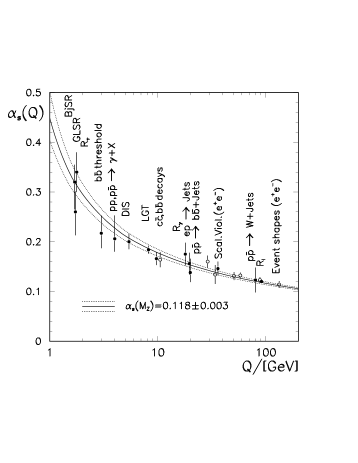
Figure 1.1: Running of the QCD coupling constant $\alpha_{s}$, for different boundary values at $\mu=m_{Z}$. The QCD prediction is compared to current experiments. (Reproduced from Ref. [37].)

In order to determine the coupling constant we have to calculate at least one physical quantity, e.g. a total scattering cross section, and compare the calculation with the measurement of the cross section. In practice, the calculation is necessarily truncated at a certain finite order. For the truncated series to be a good approximation of the full sum, the expansion variable, the coupling constant, has to be small. We also want to keep the logarithms of the renormalization scale in the coefficients of the expansion small. These two conditions constrain the value of the renormalization scale close to the typical physical scale of the process at hand. Fig. 1.1 shows the running of the QCD coupling, $\alpha_{s}(Q)=g_{s}^{2}(Q)/(4\pi)$, as the function of the physical energy scale $Q=\mu$, in the experimentally accessible region for the boundary values $\alpha_{s}(m_{Z})=0.118\pm 0.003$. The running, predicted by QCD, is in agreement with the experiments within the uncertainties. From our argument it is non-trivial that $\alpha_{s}(\mu)$ is a smooth function of the energy, since the value of the coefficient $\beta_{1}$ is changing abruptly as the function of $N_{f}$ at every quark mass threshold. The continuous definition of $\alpha_{s}(\mu)$ is achieved by requiring a non-continuous $\Lambda$ parameter. The $\Lambda$ parameter in QCD, $\Lambda_{QCD}(N_{f},N_{order})$, becomes the function of the number of active ($m_{q}<\mu$) quark flavors $N_{f}$, and the perturbative order $N_{order}$, up to which the $\beta$ function was calculated, to ensure a smooth matching at the quark thresholds. As an example we show a set of $\Lambda_{QCD}(N_{f},N_{order})/$GeV values which is recently in use [38]:

$$\begin{array}[]{rrrrr}\vspace{0.2 cm}\hfil&N_{f}=3&N_{f}=4&N_{f}=5&N_{f}=6\\ \vspace{0.2 cm}N_{order}=1&0.272&0.236&0.181&0.094\\ N_{order}=2&0.354&0.298&0.202&0.081\end{array}$$

The running coupling is one of the simplest examples of a resummed quantity. It is calculated by the reorganization of the perturbative series, such that the largest all order contributions are included in the new leading terms. The partial summation of the perturbative series implemented in this fashion is called resummation, which is the main theme of this work. Since the running coupling is a resummed quantity, when used in a fixed order expression it automatically includes certain all order effects in the calculation, and as such, it improves the quality of the prediction.

1.2.3 Factorization and Infrared Safety

The QCD Lagrangian describes the interaction of quarks and gluons. On the other hand, because of confinement, we observe only hadrons. According to the parton model [39], hadrons are composed from partons: quarks and gluons. Although, numerical implementations of QCD suggest that the theory describes confinement, we do not have a mechanism to derive low energy (long distance) properties from the QCD Lagrangian. In order to describe interactions involving hadrons at high energies we use the tool of factorization. Factorization is the idea of the separation of the short distance physics from the long distance physics in high energy collisions. The short distance physics is described by perturbative QCD. The long distance effects are showed to be universal, parametrized, and extracted from measurements.

In order to illustrate the plausibility of factorization in $hadronic$ scattering cross sections, we first highlight the calculation of $partonic$ cross sections. When calculating a partonic cross section beyond the leading order, after UV renormalization, and cancellation of the IR singularities between real emission and virtual diagrams the cross section still contains collinear singularities. These collinear singularities, on the other hand, can be isolated as multiplicative factors, just like in the case of UV renormalization. Similarly to Eq. 1.4, the partonic scattering cross section can be written as

$$d\sigma_{a_{1}a_{2}\to X}(\{s\})=\int_{0}^{1}dx_{1}\int_{0}^{1}dx_{2}\,\phi_{b_{1}/a_{1}}(x_{1},\mu)\,d\hat{\sigma}_{b_{1}b_{2}\to X}(\{s\},x_{1},x_{2},\mu)\,\phi_{b_{2}/a_{2}}(x_{2},\mu),$$ (1.6)

where summation over the double partonic indices $b_{i}$ is implied, $\hat{\sigma}_{b_{1}b_{2}\to X}$ is the hard scattering cross section of two partons $b_{1}$ and $b_{2}$, and $\phi_{b/a}(x,\mu)$ can be interpreted as the probability of the collinear emission of parton $b$ from parton $a$ with a momentum fraction $x$ at energy $\mu$, and $\{s\}$ represents the collection of the kinematical variables relevant to $d\hat{\sigma}$ (e.g. the center of mass energy of the collision, etc.), and $X$ is some arbitrary final state. The hard cross section $\hat{\sigma}_{b_{1}b_{2}\to X}$ and the distributions $\phi_{b/a}$ are calculable in perturbative QCD order by order. The above form is useful because, as it can be shown by direct calculation for a given process, all the non-cancelling infrared singularities associated with the emission of collinear partons are universal and can be defined into the distributions $\phi_{b/a}$ and the hard scattering cross section $\hat{\sigma}_{b_{1}b_{2}\to X}$ is infrared safe (i.e. finite). When calculating $\hat{\sigma}_{b_{1}b_{2}\to X}$ at higher orders of the perturbation theory, its infrared safety can be maintained by absorbing its collinear singularities into the distributions $\phi_{b/a}$ [40]. In this procedure there is a freedom of shifting part of the hard cross section into the distributions. This introduces the factorization scale, $\mu$, dependence into the definition of both $\hat{\sigma}_{b_{1}b_{2}\to X}$ and $\phi_{b/a}$. Just like in the case of the UV renormalization, there are different scheme choices for the parton densities, depending on the amount of the finite contributions arbitrarily defined into $\phi_{b/a}$. This factorization of the infrared behavior is a factorization of the short and long-distance physics, because the fact that $\hat{\sigma}_{b_{1}b_{2}\to X}$ is infrared safe implies that it cannot depend on physics which is associated by long distances. The long distance physics is described by the universal distributions $\phi_{b/a}$, which can be shown to be independent of the short distance features captured by $\hat{\sigma}_{b_{1}b_{2}\to X}$.

We can show by explicit calculation that Eq. (1.6) generalizes to hadronic cross sections:

$$d\sigma_{h_{1}h_{2}\to X}(\{s\})=\int_{0}^{1}dx_{1}\int_{0}^{1}dx_{2}\,f_{b_{1}/h_{1}}(x_{1},\mu)\,d\hat{\sigma}_{b_{1}b_{2}\to X}(\{s\},x_{1},x_{2},\mu)\,f_{b_{2}/h_{2}}(x_{2},\mu),$$ (1.7)

where $f_{a/h}(x,\mu)$ is a universal (process independent) function which gives the probability of finding parton $a$ in a $hadron$ $h$ with a momentum fraction of $x$ at the scale $\mu$. (While the introduction of the partonic distributions is somewhat heuristic in the parton model, they are defined formally in the operator product expansion in terms of expectation values of non-local operators.) The factorization theorem [41], generally formulated in Eqs. (1.6) and (1.7) is an assumption, until it is proven process by process, and order by order of the perturbation theory that the infrared singularities of the hard cross section can be factorized into the parton distributions, and an infrared safe hard cross section can be defined. The proofs are given in the literature for the most important processes as deep inelastic scattering or the Drell-Yan lepton pair production. After it is proven, the factorization theorem is used to predict cross sections involving hadrons. Comparing these predictions to the experiments, the parton distributions then can be extracted.

Although, presently we do not know how to calculate the parton distribution functions of hadrons, $f_{a/h}(x,\mu)$, from the first principles, since their scale dependence is governed by perturbative QCD, based on the RG technique we can calculate their evolution with the energy scale $\mu$:

$$\mu\frac{df_{a/h}(x,\mu)}{d\mu}=\int_{0}^{1}\frac{d\xi}{\xi}P_{a\leftarrow b}\left(\frac{x}{\xi},\alpha_{s}(\mu)\right)f_{b/h}(\xi,\mu),$$

where the splitting functions, $P_{a\leftarrow b}(x,\alpha_{s}(\mu))$, are calculable order by order of the perturbation theory [42], since they describe the short distance physics of partonic splitting. (The analog of this equation can be written for partonic distributions $\phi_{b/a}$, where the splitting functions are calculated by perturbative methods.) For the case of gluon radiation their ${\cal O}(\alpha_{s})$ expressions are:

$$P_{{j\leftarrow k}}^{(1)}(z) = C_{F}\left({\frac{1+z^{2}}{{1-z}}}\right)_{+},$$

$$P_{{j\leftarrow G}}^{(1)}(z) = {\frac{1}{2}}\left[z^{2}+(1-z)^{2}\right],$$ (1.8)

where the “+” prescription for arbitrary functions $f(z)$ and $g(z)$ is defined as

$$\int_{x}^{1}dz\left(f(z)\right)_{+}g(z)=\int_{0}^{1}dz\;f(z)\left[\Theta(z-x)g(z)-g(1)\right],$$

with

$$\Theta(x)=\cases{~{}0,&{\rm if} $x<0$,\cr~{}1,&{\rm if} $x\geq 0$,}$$

the unit step function. (It is assumed that $f(z)$ is less singular than $1/(1-z)^{2}$ at $z=1$.) Similarly to the case of the running coupling, the parton distributions, being solutions of the above RGE, include resummed collinear contributions.

The renormalization of the ultraviolet singularities and the factorization of the infrared divergences can be viewed in parallel [43]. The ultraviolet singularities absorbed into the renormalization constants $Z_{i}$, just like the collinear divergences absorbed into the parton distributions $f_{a/b}$, that is in the factorization the parton distributions play the role of the renormalization constants, with the added complication that they also depend on the momentum fraction $x$, besides the energy scale $\mu$. The evolution equations, describing the scale dependence of the renormalization constants and the parton distributions can also be casted into analogous forms, with the anomalous dimensions $\gamma_{i}$ identified with the splitting functions $P_{a\leftarrow b}$.

Chapter 2 Soft Gluon Resummation

2.1 Lepton Pair Production at Fixed Order in $\alpha_{s}$

In this work we apply and extend the resummation formalism developed by Collins, Soper and Sterman (CSS) [44, 45, 46], which resums large logarithmic contributions, arising as the consequence of the initial state multiple soft gluon emission. We calculate these resummed corrections to processes of the type $h_{1}h_{2}\rightarrow v_{1}v_{2}X$, where $h_{i}$ are hadrons, $v_{1}$ and $v_{2}$ is a pair of leptons, photons or $Z^{0}$ bosons, and $X$ is anything else produced in the collision undetected. More specifically, we consider lepton pair production through electroweak vector boson production and decay: $h_{1}h_{2}\rightarrow V(\rightarrow\ell_{1}{\bar{\ell}_{2})}X$ ($V$ is $W^{\pm}$, $Z^{0}$ or a virtual photon), and vector boson pair production $h_{1}h_{2}\rightarrow VVX$ with $V$ being photon or $Z^{0}$ boson. To resum the contributions from the soft gluon radiation, we use the results of the various fixed order calculations of these processes, which are found in the literature [47, 48, 49, 50, 51]. In this Chapter we review the lepton pair production through $W^{\pm}$, $Z^{0}$ or virtual photon ($\gamma^{*}$) production and decay in some detail, to introduce a pedagogical example identifying technical details which are most important for the resummation calculation.

2.1.1 The Collins-Soper Frame

Since the Collins-Soper-Sterman resummation formalism gives the cross sections in a special frame, called the Collins-Soper ($CS$) frame [52], we give the detailed form of the Lorentz transformation between the $CS$ and the laboratory ($lab$) frames. The $lab$ frame is defined as the center-of-mass frame of the colliding hadrons $h_{1}$ and $h_{2}$. In the $lab$ frame, the cartesian coordinates of the hadrons are:

$$p_{h_{1},h_{2}}^{\mu}(lab)=\frac{\sqrt{S}}{2}\,(1,0,0,\pm 1),$$

where $\sqrt{S}$ is the center-of-mass energy of the collider. The $CS$ frame is the special rest frame of the vector boson in which the $z$ axis bisects the angle between the $h_{1}$ hadron momentum $p_{h_{1}}(CS)$ and the negative $h_{2}$ hadron momentum $-p_{h_{2}}(CS)$ [53].

To derive the Lorentz transformation $\Lambda_{~{}\nu}^{\mu}(lab\rightarrow CS)$ that connects the $lab$ and $CS$ frames (in the active view point):

$$p^{\mu}(CS)=\Lambda_{~{}\nu}^{\mu}(lab\rightarrow CS)\;p^{\nu}(lab),$$

we follow the definition of the $CS$ frame. Since the invariant amplitude is independent of the azimuthal angle of the vector boson ($\phi_{V}$), without loosing generality we start from a $lab$ frame in which $\phi_{V}$ is zero. First, we find the boost into a vector boson rest frame. Then, in the vector boson rest frame we find the rotation which brings the hadron momentum $p_{h_{1}}(CS)$ and negative hadron momentum $-p_{h_{2}}(CS)$ into the desired directions.

A boost by $\vec{\beta}=-\vec{q}(lab)/q^{0}$ brings four vectors from the lab frame (with $\phi_{V}=0$) into a vector boson rest frame ($rest$). The matrix of the Lorentz boost from the $lab$ frame to the $rest$ frame, expressed explicitly in terms of $q^{\mu}$ is

$$\Lambda_{~{}\nu}^{\mu}(lab\rightarrow rest)=$$

$${\frac{1}{Q}}\left(\begin{tabular}[]{rrrr}$q^{0}$&$-Q_{T}$&$0$&$-q^{3}$\\ $-Q_{T}$&$Q+{\frac{Q_{T}^{2}}{q^{0}+Q}}$&$0$&${\frac{Q_{T}q^{3}}{q^{0}+Q}}$\\ $0$&${0}$&$Q$&${0}$\\ $-q^{3}$&${\frac{Q_{T}q^{3}}{q^{0}+Q}}$&$0$&$Q+\frac{(q^{3})^{2}}{q^{0}+Q}$\end{tabular}\right).$$

where $Q=\sqrt{(q^{0})^{2}-Q_{T}^{2}-(q^{3})^{2}}$ is the vector boson invariant mass, and the transverse mass is defined as $M_{T}=\sqrt{Q^{2}+Q_{T}^{2}}$.

After boosting the lab frame hadron momenta into this rest frame, we obtain

$$p_{h_{1},h_{2}}^{\mu}(rest) = \Lambda_{~{}\nu}^{\mu}(lab\rightarrow rest)\;p_{h_{1},h_{2}}^{\nu}(lab)=$$

$$\frac{\sqrt{S}}{2}\left(\frac{q^{0}\mp q^{3}}{Q},-\frac{Q_{T}}{Q}\frac{q^{0}+Q\mp q^{3}}{q^{0}+Q},0,\frac{(\pm Q-q^{3})(q^{0}+Q)\pm(q^{3})^{2}}{Q(q^{0}+Q)}\right),$$

and the polar angles of $p_{h_{1}}^{\mu}(rest)$ and $-p_{h_{2}}^{\mu}(rest)$ are not equal unless $Q_{T}=0$. (In the above expressions the upper signs refers to $h_{1}$ and the lower signs to $h_{2}$.) In the general $Q_{T}\neq 0$ case we have to apply an additional rotation in the $rest$ frame so that the $z$-axis bisects the angle between the hadron momentum $p_{h_{1}}(CS)$ and the negative hadron momentum $-p_{h_{2}}(CS)$. It is easy to verify that to keep $\vec{p}_{h_{1},h_{2}}$ in the $xz$ plane, this rotation should be a rotation around the $y$ axis by an angle $\alpha=\arccos{[Q(q^{0}+M_{T})/(M_{T}(q^{0}+Q))]}$.

Thus the Lorentz transformation from the $lab$ frame to the $CS$ frame is $\Lambda_{~{}\nu}^{\mu}(lab\rightarrow CS)=\Lambda_{~{}\lambda}^{\mu}(rest\rightarrow CS)\;\Lambda_{~{}\nu}^{\lambda}(lab\rightarrow rest)$. Indeed, this transformation results in equal polar angles $\theta_{h_{1},-h_{2}}=\arctan(Q_{T}/Q)$. The inverse of this transformation takes vectors from the $CS$ frame to the $lab$ frame is:

$$\Lambda_{~{}\nu}^{\mu}(CS \rightarrow lab)=\left(\Lambda_{~{}\nu}^{\mu}(lab\rightarrow CS)\right)^{-1}=$$

$${\frac{1}{QM_{T}}}\left(\begin{tabular}[]{rrrr}$q^{0}M_{T}$&$q^{0}Q_{T}$&$0$&$q^{3}Q$\\ $Q_{T}M_{T}$&$M_{T}^{2}$&$0$&$0$\\ $0$&$0$&$QM_{T}$&$0$\\ $q^{3}M_{T}$&$q^{3}Q_{T}$&$0$&$q^{0}Q$\end{tabular}\right).$$

The kinematics of the leptons from the decay of the vector boson can be described by the polar angle $\theta$ and the azimuthal angle $\phi$, defined in the Collins-Soper frame. The above transformation formulae lead to the four-momentum of the decay product fermion (and anti-fermion) in the lab frame as

$$p^{\mu} = {\frac{Q}{2}}\left({\frac{q^{\mu}}{Q}}+\sin{\theta}\cos{\phi}~{}X^{\mu}+\sin{\theta}\sin{\phi}~{}Y^{\mu}+\cos{\theta}~{}Z^{\mu}\right),$$

$$\overline{p}^{\mu} = q^{\mu}-p^{\mu},$$

where

$$q^{\mu}=(M_{T}\cosh{y},\,Q_{T}\cos{\phi_{V}},\,Q_{T}\sin{\phi_{V}},\,M_{T}\sinh{y}),$$

$$X^{\mu}=-{\frac{Q}{Q_{T}M_{T}}}\left(q_{+}n^{\mu}+q_{-}{\bar{n}}^{\mu}-{\frac{M_{T}^{2}}{Q^{2}}}q^{\mu}\right),$$

$$Z^{\mu}={\frac{1}{M_{T}}}\left(q_{+}n^{\mu}-q_{-}{\bar{n}}^{\mu}\right),$$

$$Y^{\mu}=\varepsilon^{\mu\nu\alpha\beta}{\frac{q_{\nu}}{Q}}Z_{\alpha}X_{\beta}.$$ (2.3)

Here, $q_{\pm}={\frac{1}{\sqrt{2}}}(q^{0}\pm q^{3})$, $y=\frac{1}{2}\ln(q_{+}/q_{-})$, $n^{\nu}=\frac{1}{\sqrt{2}}(1,0,0,1)$, ${\bar{n}}^{\nu}={\frac{1}{\sqrt{2}}}(1,0,0,-1)$ and the totally anti-symmetric unit tensor is defined as $\varepsilon^{0123}=-1$.

2.1.2 General Properties of the Cross Section

Along the lines of the factorization theorem (cf. Eq. 1.7), the inclusive differential cross section of the lepton pair production in a hadron collision process $h_{1}h_{2}\to V(\to\ell_{1}{\bar{\ell}_{2}})X$ is written as

$$d\sigma_{h_{1}h_{2}}(Q,Q_{T},y,\theta,\phi,\alpha_{s}(Q))=$$

$$~{}~{}~{}\int_{x_{1}}^{1}d\xi_{1}\int_{x_{2}}^{1}d\xi_{2}\sum_{a,b}\;\,f_{a/h_{1}}(\xi_{1},\mu)\,\;d\hat{\sigma}_{ab}(Q,Q_{T},y,\theta,\phi,z_{1},z_{2},\mu)\;\,f_{b/h_{2}}(\xi_{2},\mu).$$

Here $d\hat{\sigma}_{ab}$ is the differential cross section of the parton level process $ab\to V(\to\ell_{1}{\bar{\ell}_{2}})X$, and $f_{a/h}$ are the parton distribution functions. The variable $Q$ denotes the invariant mass, $y$ the rapidity and $Q_{T}$ the transverse momentum of the lepton pair, while $\theta$ and $\phi$ are the polar and azimuthal angles of the lepton $\ell_{1}$ in the rest frame of $V$. The indices $a$ and $b$ denote different parton flavors (including gluon), and $V$ may stand for $W^{\pm}$, $Z^{0}$ or $\gamma^{*}$. The partonic momentum fractions $x_{i}$ are related to these independent variables as

$$x_{1}=\frac{M_{T}}{\sqrt{S}}e^{y},\;\;\;x_{2}=\frac{M_{T}}{\sqrt{S}}e^{-y},$$

and

$$z_{1,2}={\frac{x_{1,2}}{\xi_{1,2}}.}$$

The partonic cross section $\hat{\sigma}_{ab}$ is calculated as

$$d\hat{\sigma}_{ab}(Q,Q_{T},y,\theta,\phi,x_{1},x_{2},\mu)=\frac{1}{2s}\overline{\left|{\cal M}_{ab}(s,t,u,\mu)\right|^{2}}d\Phi.$$

where $s$, $t$, and $u$ are the Mandelstam invariants

$$s=(p_{a}+p_{b})^{2},\;\;\;t=(p_{a}-Q)^{2},\;\;\;u=(p_{b}-Q)^{2}$$

with $p_{a}$ and $p_{b}$ being the four momenta of the incoming partons, and $Q$ is the four momentum of the lepton pair. Momentum conservation, $p_{a}+p_{b}=Q+p_{X}$, can be expressed in the form of the Mandelstam relation

$$s+t+u=Q^{2},$$

where we used $p_{X}^{2}=0$. The phase space factor $d\Phi$, assuming massless leptons, in terms of the relevant kinematical variables, is

$$d\Phi=\frac{1}{2^{9}\pi^{4}}\;\delta(s+t+u-Q^{2})\;dQ^{2}dQ_{T}^{2}dyd\cos\theta d\phi.$$

The averaged square of the invariant amplitude

$$\overline{\left|{\cal M}_{ab}(s,t,u,\mu)\right|^{2}}=\frac{1}{n_{a}^{c}n_{b}^{c}n_{a}^{s}n_{b}^{s}}\sum_{colors}\left|{\cal M}_{ab}(s,t,u,\mu_{f})\right|^{2},$$

where $n_{a,b}^{s}$ and $n_{a,b}^{c}$ are the number of spin and color degrees of freedom of partons $a$ and $b$.

Using the relation $s=\xi_{1}\xi_{2}S$, where $\sqrt{S}$ is the center of mass energy of the collider, the differential cross section of the lepton pair production in a fixed order of the strong coupling is written as

$${\left({\frac{d\sigma(h_{1}h_{2}\rightarrow V(\rightarrow\ell_{1}{\bar{\ell}_{2}})X)}{dQ^{2}dQ_{T}^{2}dyd\cos{\theta}d\phi}}\right)}_{{\rm Fixed}}=\frac{1}{2^{10}\pi^{4}S}\sum_{a,b}\int_{x_{1}}^{1}{\frac{d\xi_{1}}{\xi_{1}}}\int_{x_{2}}^{1}{\frac{d\xi_{2}}{\xi_{2}}}$$

$$~{}~{}~{}\times~{}\,f_{a/h_{1}}(\xi_{1},\mu)\overline{\left|{\cal M}_{ab}(s,t,u,\mu)\right|^{2}}\delta(s+t+u-Q^{2})\,f_{b/h_{2}}(\xi_{2},\mu).$$

In the above equation both the invariant amplitude ${\cal M}_{ab}(s,t,u,\mu)$ and the parton distribution functions $f_{a/h}(x,\mu)$ depend on the renormalization scale

$$\mu=C_{4}Q$$

and the corresponding value, $g_{s}(\mu)=\sqrt{4\pi\alpha_{s}(\mu)}$, of the QCD coupling. Normally one sets the constant $C_{4}$ to be of order 1, to avoid large logarithms $\ln(Q/\mu)$, that would otherwise spoil the usefulness of a low–order perturbative approximation of ${\cal M}_{ab}$.

The squared invariant amplitude of the partonic level process is calculated contracting the hadronic and leptonic tensors $H^{\mu\nu}$ and $L_{\mu\nu}$:

$$\left|{\cal M}_{ab}(s,t,u,Q^{2})\right|^{2}=H_{ab}^{\mu\nu}(k,l,Q)L_{\mu\nu}(l_{1},l_{2},Q)$$

where, for the $q\bar{q}\rightarrow V(\rightarrow\ell_{1}{\bar{\ell}_{2}})g$ process $k,l,l_{1},l_{2}$ are the quark, anti-quark, lepton and anti-lepton four-momenta, respectively. The detailed from of the hard cross section is found in the next Section. The hadronic tensor $H_{ab}$ is calculated by evaluating the ${\cal O}(\alpha_{s})$ real and virtual gluon emission diagrams and adding together these contributions. In order to keep track of the vector boson polarization one has to evaluate the symmetric and anti-symmetric parts of both the hadronic and leptonic tensors. Since the calculation of the leptonic tensor is trivial we focus on the hadronic tensor.

The hadronic tensor can be split into a sum of a symmetric and an anti-symmetric tensor

$$H_{ab}^{\mu\nu}(k,l,Q)=H_{ab,S}^{\mu\nu}(k,l,Q)+H_{ab,A}^{\mu\nu}(k,l,Q).$$

Here $H_{ab,S}^{\mu\nu}(k,l,Q)$ depends on symmetric combinations of the four-momenta and the metric tensor. The calculation of the symmetric part of the hadronic tensor $H_{ab,S}^{\mu\nu}(k,l,Q)$ is straightforward and does not depend on the prescription of the $\gamma_{5}$. This is because one does not have to evaluate a trace that contains $\gamma_{5}$ to calculate $H_{ab,S}^{\mu\nu}(k,l,Q)$. But the anti-symmetric part of the hadronic tensor involves traces containing single $\gamma_{5}$’s. These traces are, by definition, proportional to the fully anti-symmetric tensor $\varepsilon^{\mu\nu\alpha\beta}$, so that the calculation of $H_{ab,A}^{\mu\nu}(k,l,Q)$ lead to the form

$$H_{ab,A}^{\mu\nu}(k,l,Q)=h_{1}(s,t,u,Q^{2})\varepsilon^{\mu\nu kQ}+h_{2}(s,t,u,Q^{2})\varepsilon^{\mu\nu lQ}+\epsilon\;h_{3}(s,t,u,Q^{2})\varepsilon^{\mu\nu kl}.$$

The last term in this equation would violate the Ward identities in four dimension. Although proportional to $\epsilon=(4-D)/2$, after the phase-space integration it contributes to the four-dimensional cross section if $h_{3}$ does not vanish.

2.1.3 The Cross Section at ${\cal O}(\alpha_{s})$

To correctly extract the distributions of the leptons, we have to calculate the production and the decay of a polarized vector boson. The ${\cal O}(\alpha_{s})$ QCD corrections to the production and decay of a polarized vector boson can be found in the literature [48], in which both the symmetric and the anti-symmetric parts of the hadronic tensor were calculated. Such a calculation was, as usual, carried out in general number ($D$) of space-time dimensions, and dimensional regularization was used to regulate infrared (IR) divergences because it preserves the gauge and the Lorentz invariances. Since the anti-symmetric part of the hadronic tensor contains traces with an odd number of $\gamma_{5}$’s, one has to choose a definition (prescription) of $\gamma_{5}$ in $D$ dimensions. It was shown in a series of papers [54, 55] that in $D\neq 4$ dimension, the consistent $\gamma_{5}$ prescription to use is the t’Hooft-Veltman prescription [54]. Since in Ref. [48] a different prescription [56] was used, we give below the results of our calculation in the t’Hooft-Veltman $\gamma_{5}$ prescription.

For calculating the virtual corrections, we follow the argument of Ref. [57] and impose the chiral invariance relation, which is necessary to eliminate ultraviolet anomalies of the one loop axial vector current when calculating the structure function. Applying this relation for the virtual corrections we obtain the same result as that in Refs. [48] and [58]. The final result of the virtual corrections gives

$${\cal M}_{Born}^{\dagger}{\cal M}_{Virt}+{\cal M}_{Virt}^{\dagger}{\cal M}_{Born}=$$

$$~{}~{}~{}~{}~{}~{}~{}~{}~{}~{}C_{F}\frac{\alpha_{s}}{2\pi}\left(\frac{4\pi\mu^{2}}{Q^{2}}\right)^{\epsilon}\frac{1}{\Gamma(1-\epsilon)}\left(-\frac{2}{\epsilon^{2}}-\frac{3}{\epsilon}+\pi^{2}-8\right)\left|{\cal M}_{Born}\right|^{2},$$ (2.4)

where $\epsilon=(4-D)/2$, $\mu$ is the t’Hooft mass (renormalization) scale, and $C_{F}=4/3$ in QCD. The four-dimensional Born level amplitude is

$$\left|{\cal M}_{Born}\right|^{2} = {\frac{16Q^{4}}{(Q^{2}-M_{V}^{2})^{2}+Q^{4}\Gamma_{V}^{2}/M_{V}^{2}}}$$ (2.5)

$$\times\left[(g_{L}^{2}+g_{R}^{2})(f_{L}^{2}+f_{R}^{2}){\cal L}_{0}+(g_{L}^{2}-g_{R}^{2})(f_{L}^{2}-f_{R}^{2}){\cal A}_{3}\right],$$

where we have used the LEP prescription for the vector boson resonance with mass $M_{V}$ and width $\Gamma_{V}$. The angular functions are ${\cal L}_{0}=1+\cos^{2}{\theta}$ and ${\cal A}_{3}=2\cos{\theta}$. The initial state spin average (1/4), and color average (1/9) factors are not yet included in Eq. (2.5).

When calculating the real emission diagrams, we use the same (t’Hooft-Veltman) $\gamma_{5}$ prescription. It is customary to organize the ${\cal O}(\alpha_{s}^{n})$ corrections by separating the lepton degrees of freedom from the hadronic ones, so that

$${\left({\frac{d\sigma(h_{1}h_{2}\rightarrow V(\rightarrow\ell_{1}{\bar{\ell}_{2}})X)}{dQ^{2}dydQ_{T}^{2}d\cos{\theta}d\phi}}\right)}_{{\cal O}(\alpha_{s})}^{{\rm real~{}emission}}={\frac{\alpha_{s}(Q)C_{F}}{(2\pi)^{3}S}}{\frac{Q^{2}}{(Q^{2}-M_{V}^{2})^{2}+Q^{4}\Gamma_{V}^{2}/M_{V}^{2}}}$$

$$~{}~{}~{}\times\sum_{a,b,i}\int_{x_{1}}^{1}{\frac{d\xi_{1}}{\xi_{1}}}\int_{x_{2}}^{1}{\frac{d\xi_{2}}{\xi_{2}}}~{}{\cal G}^{i\;}{\cal L}_{ab}(\xi_{1},\xi_{2},Q^{2})\;{\cal T}_{ab}^{i}(Q_{T},Q,z_{1},z_{2})\ {\cal A}_{i}(\theta,\phi),$$

with $z_{1}=x_{1}/\xi_{1}$ and $z_{2}=x_{2}/\xi_{2}$. The dependence on the lepton kinematics is carried by the angular functions

$${\cal L}_{0}=1+\cos^{2}{\theta},~{}{\cal A}_{0}={\frac{1}{2}}(1-3\cos^{2}{\theta}),~{}{\cal A}_{1}=\sin{2\theta}\cos{\phi},~{}{\cal A}_{2}={\frac{1}{2}}\sin^{2}{\theta}\cos{2\phi},~{}$$

$${\cal A}_{3}=2\cos{\theta},~{}{\cal A}_{4}=\sin{\theta}\cos{\phi}.$$

In the above differential cross section, $i=-1,...,4$ with ${\cal A}_{-1}\equiv{\cal L}_{0}$; and ${\cal G}^{i}=(g_{L}^{2}+g_{R}^{2})(f_{L}^{2}+f_{R}^{2})$ for $i=-1,0,1,2;$ ${\cal G}^{i}=(g_{L}^{2}-g_{R}^{2})(f_{L}^{2}-f_{R}^{2})$ for $i=3,4$. The parton level cross sections are summed for the parton indices $a$, $b$ in the following fashion

$$\sum_{a,b}{\cal L}_{ab}\;{\cal T}_{ab}^{i}=\sum_{q=u,d,s,c,b}\left({\cal L}_{q\bar{q}}\;{\cal T}_{q\bar{q}}^{i}+{\cal L}_{\bar{q}q}\;{\cal T}_{\bar{q}q}^{i}+{\cal L}_{qG}\;{\cal T}_{qG}^{i}+{\cal L}_{\bar{q}G}\;{\cal T}_{\bar{q}G}^{i}+{\cal L}_{Gq}\;{\cal T}_{Gq}^{i}+{\cal L}_{G\bar{q}}\;{\cal T}_{G\bar{q}}^{i}\right).$$

The partonic luminosity functions ${\cal L}_{ab}$ are defined as

$${\cal L}_{q\bar{q}}(\xi_{1},\xi_{2},Q^{2})=f_{q/h_{1}}(\xi_{1},Q^{2})\;f_{\bar{q}/h_{2}}(\xi_{2},Q^{2}),\;etc.,$$

where $f_{q/h_{1}}$ is the parton probability density of parton $q$ in hadron $h_{1}$, etc. The squared matrix elements for the annihilation sub-process $q{\bar{q}}\rightarrow VG$ in the $CS$ frame, including the $\epsilon$ dependent terms, are as follows:

$$\ {\cal T}_{q\bar{q}}^{-1} = \frac{1}{ut}\left(T_{+}(u,t)-(t+u)^{2}\epsilon\right),\;\;$$

$${\cal T}_{q\bar{q}}^{0}\;\; = {\cal T}_{q\bar{q}}^{2}=\frac{1}{ut}\frac{Q_{T}^{2}}{M_{T}^{2}}\left(T_{+}(u,t)-(Q^{2}+s)^{2}\epsilon\right),\;$$

$${\cal T}_{q\bar{q}}^{1}\;\; = \frac{1}{ut}\frac{Q_{T}Q}{M_{T}^{2}}T_{-}(u,t)(1-\epsilon),\;$$

$${\cal T}_{q\bar{q}}^{3}\;\; = \frac{1}{ut}\frac{Q}{M_{T}}\left(T_{+}(u,t)-{\frac{(Q^{2}-u)t^{2}+(Q^{2}-t)u^{2}}{Q^{2}}}\epsilon\right),\;$$

$${\cal T}_{q\bar{q}}^{4}\;\; = \frac{2}{ut}\frac{Q_{T}}{M_{T}}\left(T_{-}(u,t)+Q^{2}(u-t)\epsilon\right).$$

For the Compton sub-process $qG\rightarrow Vq$, we obtain

$$\ {\cal T}_{qG}^{-1} = \frac{-1}{su}\left(T_{+}(s,u)-{(s+u)^{2}}\epsilon\right),\;\;$$

$${\cal T}_{qG}^{0}\;\; = {\cal T}_{qG}^{2}=\frac{-1}{su}\frac{Q_{T}^{2}}{M_{T}^{2}}\left((Q^{2}-u)^{2}+(Q^{2}+s)^{2}-{(s+u)^{2}}\epsilon\right),$$

$$\;{\cal T}_{qG}^{1}\;\; = \frac{-1}{su}\frac{Q_{T}Q}{M_{T}^{2}}\left(2(Q^{2}-u)^{2}-(Q^{2}-t)^{2}+{(s+u)^{2}}\epsilon\right),\;$$

$${\cal T}_{qG}^{3}\;\; = \frac{-1}{su}\frac{Q}{M_{T}}\left(T_{+}(s,u)-2u(Q^{2}-s)+\frac{(Q^{2}-t)(Q^{2}s-su-u^{2})}{Q^{2}}\epsilon\right),$$

$${\cal T}_{qG}^{4}\;\; = \frac{-2}{su}\frac{Q_{T}}{M_{T}}\left(2s(Q^{2}-s)+T_{+}(s,u)-(Q^{2}-t)u\epsilon\right).$$

In the above equations, the Mandelstam variables: $s=(k+l)^{2}$, $t=(k-Q)^{2}$, and $u=(l-Q)^{2}$ where $k$, $l$ and $q$ are the four momenta of the partons from hadrons $h_{1}$, $h_{2}$ and that of the vector boson, respectively, and $T_{\pm}(t,u)=(Q^{2}-t)^{2}\pm(Q^{2}-u)^{2}$. All other necessary parton level cross sections can be obtained from the above as summarized by the following crossing rules:

$i=-1,0,1,2$	$i=3,4$
${\cal T}_{\bar{q}q}^{i}={\cal T}_{q\bar{q}}^{i}$	${\cal T}_{\bar{q}q}^{i}=-{\cal T}_{q\bar{q}}^{i}$
${\cal T}_{Gq}^{i}={\cal T}_{qG}^{i}\;(u\leftrightarrow t)\;\;\;\;\;\;\;$	${\cal T}_{Gq}^{i}=-{\cal T}_{qG}^{i}\;(u\leftrightarrow t)$
${\cal T}_{\bar{q}G}^{i}={\cal T}_{qG}^{i}$	${\cal T}_{\bar{q}G}^{i}=-{\cal T}_{qG}^{i}$
${\cal T}_{G\bar{q}}^{i}={\cal T}_{Gq}$	${\cal T}_{G\bar{q}}^{i}=-{\cal T}_{Gq}^{i},$

with the only exceptions that ${\cal T}_{Gq}^{1}=-{\cal T}_{qG}^{1}\;(u\leftrightarrow t)$ and ${\cal T}_{Gq}^{4}={\cal T}_{qG}^{4}\;(u\leftrightarrow t)$. These results are consistent with the regular pieces of the $Y$ term given in Section 2.2.5 and with those in Ref. [49].

In the above matrix elements, only the coefficients of ${\cal L}_{0}$ and ${\cal A}_{3}$ are not suppressed by $Q_{T}$ or $Q_{T}^{2}$, so they contribute to the singular pieces which are resummed in the CSS formalism. By definition we call a term singular if it diverges as $Q_{T}^{-2}$ $\times$ [1 or $\ln(Q^{2}/Q_{T}^{2})$] as $Q_{T}\rightarrow 0$. Using the t’Hooft-Veltman prescription of $\gamma_{5}$ we conclude that the singular pieces of the symmetric (${\cal L}_{0}$) and anti-symmetric (${\cal A}_{3}$) parts are the same, and

$$\lim\limits_{Q_{T}\rightarrow 0}\ {\cal T}_{q\bar{q}}^{-1}\;\delta(s+t+u-Q^{2}) = \lim\limits_{Q_{T}\rightarrow 0}\ {\cal T}_{q\bar{q}}^{3}\;\delta(s+t+u-Q^{2})={s}_{q\bar{q}},$$

$$\lim\limits_{Q_{T}\rightarrow 0}\ {\cal T}_{Gq}^{-1}\;\delta(s+t+u-Q^{2}) = \lim\limits_{Q_{T}\rightarrow 0}\ {\cal T}_{Gq}^{3}\;\delta(s+t+u-Q^{2})={s}_{Gq},$$

where

$${s}_{q\bar{q}} = \frac{1}{Q_{T}^{2}}\left[2\;\delta(1-z_{1})\;\delta(1-z_{2})\left(\ln\frac{Q^{2}}{Q_{T}^{2}}-\frac{3}{2}\right)\right.$$

$$\left.+\delta(1-z_{1})\left(\frac{1+z_{2}{}^{2}}{1-z_{2}}\right)_{+}+\delta(1-z_{2})\left(\frac{1+z_{1}{}^{2}}{1-z_{1}}\right)_{+}\right.$$

$$\left.-\left((1-z_{1})\;\delta(1-z_{2})+(1-z_{2})\;\delta(1-z_{1})\right)\epsilon\right]+{\cal O}\left({\frac{1}{Q_{T}}}\right),$$

$${s}_{Gq} = \frac{1}{Q_{T}^{2}}\left[(z_{1}^{2}+\ (1-z_{1}^{2}))\;\delta(1-z_{2})-\delta(1-z_{2})\epsilon\right]+{\cal O}\left({\frac{1}{Q_{T}}}\right).$$

As $Q_{T}\rightarrow 0$, only the ${\cal L}_{0}$ and ${\cal A}_{3}$ helicity cross sections survive as expected, since the ${\cal O}(\alpha_{s}^{0})$ differential cross section contains only these angular functions [cf. Eq. (2.5)].

2.2 The Resummation Formalism

2.2.1 Renormalization Group Analysis

In hard scattering processes, the dynamics of the multiple soft–gluon radiation is predicted by resummation [59]–[60]. Since our work is based on the Collins-Soper-Sterman resummation formalism [44, 45, 46], in this Section we review the most important details of the proof of this formalism. After the pioneering work of Dokshitser, D’Yakonov, and Troyan [61], it was proven by Collins and Soper in Ref. [44] that besides the leading logarithms [62] all the large logarithms, including the sub-logs in the order-by-order calculations, can be expressed in a closed form (resummed) for the energy correlation in $e^{+}e^{-}$ collisions. This proof was generalized to the single vector boson $V$ production process $h_{1}h_{2}\rightarrow VX$, which we consider as an example. Generalization of the results to other processes is discussed later.

As a first step, using the factorization theorem, the cross section of the process is written in a general form

$${{\frac{d\sigma(h_{1}h_{2}\rightarrow VX)}{dQ^{2}dQ_{T}^{2}dy}}}=$$

$$~{}~{}~{}\int_{x_{1}}^{1}{\frac{d\xi_{1}}{\xi_{1}}}\int_{x_{2}}^{1}{\frac{d\xi_{2}}{\xi_{2}}}\sum_{a,b}f_{a/h_{1}}(\xi_{1},\mu)\;T_{ab}(Q,Q_{T},z_{1},z_{2},\mu_{f})\;f_{b/h_{2}}(\xi_{2},\mu).$$

The hard part of the cross section is calculated order by order in the strong coupling

$$T_{ab}(Q,Q_{T},z_{1},z_{2},\mu)=\sum_{n=0}^{\infty}\left(\frac{\alpha_{s}}{\pi}\right)^{n}T_{ab}^{(n)}(Q,Q_{T},z_{1},z_{2},\mu).$$

At some fixed order in $\alpha_{s}$ the coefficients $T_{ab}^{(n)}$ can be split into singular and regular parts

$$T_{ab}^{(n)}(Q,Q_{T},z_{1},z_{2},\mu)=T_{ab}^{(n,\delta)}(Q,Q_{T},z_{1},z_{2},\mu)\delta(Q_{T})+$$

$$~{}~{}~{}\sum_{m=0}^{2n-1}T_{ab}^{(n,m)}(Q,Q_{T},z_{1},z_{2},\mu)\frac{1}{Q_{T}^{2}}\ln^{m}\left(\frac{Q^{2}}{Q_{T}^{2}}\right)+R_{ab}^{(n)}(Q,Q_{T},z_{1},z_{2},\mu)$$

where $R_{ab}^{(n)}$ contains terms which are less singular than $Q_{T}^{-2}$ and $\delta(Q_{T})$ as $Q_{T}\rightarrow 0$. The perturbative expansion of the cross section defined in this manner is not useful when $\alpha_{s}^{n}Q_{T}^{-2}\ln^{m}\left(Q^{2}/Q_{T}^{2}\right)$ is large, i.e. in the $Q_{T}\rightarrow 0$ limit. This is expressed in saying that the large log’s are not under control when the perturbative series is calculated in terms of $T_{ab}^{(n)}$.

To gain control over these large log’s, that is to express the cross section in terms of coefficients which do not contain large log’s, the summation of the perturbative terms is reorganized. The cross section is rewritten in the form

$${\frac{d\sigma(h_{1}h_{2}\rightarrow VX)}{dQ^{2}\,dQ_{T}^{2}dy\,\,}}={\frac{1}{(2\pi)^{2}}}\int d^{2}b\,e^{i{\vec{Q}_{T}}\cdot{\vec{b}}}{\widetilde{W}(b,Q,x_{1},x_{2})}+~{}Y(Q_{T},Q,x_{1},x_{2})$$

where ${\widetilde{W}(b,Q,x_{1},x_{2})}$ accommodates the singular logarithmic terms in the form of $\ln(b^{2}Q^{2})$. The ”regular” terms are included in the $Y$ piece

$$Y(Q_{T},Q,x_{1},x_{2})=$$

$$~{}~{}~{}\int_{x_{1}}^{1}{\frac{d\xi_{1}}{\xi_{1}}}\int_{x_{2}}^{1}{\frac{d\xi_{2}}{\xi_{2}}}~{}\,f_{a/h_{1}}(\xi_{1},\mu)\;\sum_{n=0}^{\infty}\left(\frac{\alpha_{s}}{\pi}\right)^{n}R_{ab}^{(n)}(Q,Q_{T},z_{1},z_{2},\mu)\;\,f_{b/h_{2}}(\xi_{2},\mu).$$

The Fourier integral form was introduced to explicitly conserve ${\vec{Q}_{T}}$ [62].

Based on the form of the singular pieces in the $Q_{T}\rightarrow 0$ limit [46], it is assumed that the $x_{1}$ and $x_{2}$ dependence of $\widetilde{W}$ factorizes

$${\widetilde{W}(Q,b,x_{1},x_{2})}=\sum_{j}{\cal C}_{jh_{1}}(Q,b,x_{1})\;{\cal C}_{jh_{2}}(Q,b,x_{2})\;Q_{j}^{2},$$

where ${\cal C}_{jh}$ is a convolution of the parton distribution with a calculable Wilson coefficient, called $C$ function

$${\cal C}_{jh}(Q,b,x)=\sum_{a}\int_{x}^{1}{\frac{d\xi}{\xi}}\;C_{ja}(\frac{x}{\xi},b,\mu,Q)\;f_{a/h}(\xi,\mu),$$

where $a$ sums over incoming partons, and $j$ denotes the quark flavors with charge $Q_{j}$ in the units of the positron charge.

It is argued , based on the work in Ref. [45], that $\widetilde{W}$ obeys the evolution equation

$$\frac{\partial}{\partial\ln Q^{2}}{\widetilde{W}(Q,b,x_{1},x_{2})=}\left[{K}\left({b\mu,g}_{s}(\mu)\right){+G}\left({Q/\mu,g}_{s}(\mu)\right)\right]{\widetilde{W}(Q,b,x_{1},x_{2})},$$

where ${K}\left({b\mu,g}_{s}(\mu)\right)$ and ${G}\left({Q/\mu,g}_{s}(\mu)\right)$ satisfy the renormalization group equations (RGE’s)

$$\mu\frac{d}{d\mu}{K}\left({b\mu,g}_{s}(\mu)\right)=-\gamma_{K}\left({g}_{s}(\mu)\right),$$

$$\mu\frac{d}{d\mu}{G}\left({b\mu,g}_{s}(\mu)\right)=+\gamma_{K}\left({g}_{s}(\mu)\right).$$

The anomalous dimension $\gamma_{K}$ can be determined from the singular part of the cross section [63]. These RGE’s allow the control of the log’s, since using them one can change the scale ${\mu}$ in ${K}\left({b\mu,g}_{s}(\mu)\right)$ and ${G}\left({Q/\mu,g}_{s}(\mu)\right)$ independently, such that it is the order of $1/b$ and $Q$ respectively, so they do not contain large log’s. The solution of the RGE’s constructed in this fashion contain the functions $A$ and $B$, which one uses to rewrite the evolution equation of ${\widetilde{W}}$

$$\frac{\partial}{\partial\ln Q^{2}}{\widetilde{W}(Q,b,,x_{1},x_{2})}=$$

$$~{}~{}~{}\left\{\int_{C_{1}/b}^{C_{2}Q}\frac{d\overline{\mu}^{2}}{\overline{\mu}^{2}}\left[{A}\left({g}_{s}(\overline{\mu}),C_{1}\right){+B}\left({g}_{s}(C_{2}Q),C_{1},C_{2}\right)\right]\right\}{\widetilde{W}(Q,b,x_{1},x_{2})}.$$

The $A$ and $B$ functions can be approximated well, calculating them order by order in the perturbation theory, because they are free from the large log’s.

The only remaining task is to relate the $A$ and $B$ functions to the cross section. This is done by solving the evolution equation of ${\widetilde{W}}$. The solution is of the form

$${\widetilde{W}(Q,b,x_{1},x_{2})}=e^{-{\cal S}(Q,b{,C_{1},C_{2}})}{\widetilde{W}(\frac{C_{1}}{C_{2}b},b,x_{1},x_{2})},$$

where the Sudakov exponent is defined as

$${\cal S}(Q,b{,C_{1},C_{2}})=\int_{C_{1}^{2}/b^{2}}^{C_{2}^{2}Q^{2}}\frac{d\overline{\mu}^{2}}{\overline{\mu}^{2}}\left[{A}\left({g}_{s}(\overline{\mu}),C_{1}\right)\ln\left(\frac{C_{2}Q^{2}}{\overline{\mu}^{2}}\right){+B}\left({g}_{s}(\overline{\mu}),C_{1},C_{2}\right)\right].$$

From this we can write the cross section in terms of the $A$, $B$ and $C$ functions

$${\frac{d\sigma(h_{1}h_{2}\rightarrow W^{\pm}X)}{dQ^{2}\,dQ_{T}^{2}dy\,\,}}=$$

$$~{}~{}~{}{\frac{1}{(2\pi)^{2}}}\int d^{2}b\,e^{i{\vec{Q}_{T}}\cdot{\vec{b}}}\,e^{-{\cal S}(Q{,b,C_{1},C_{2}})}~{}\sum_{j}{\cal C}_{jh_{1}}(\frac{C_{1}}{C_{2}b},b,x_{1})\;{\cal C}_{jh_{2}}(\frac{C_{1}}{C_{2}b},b,x_{2})\;Q_{j}^{2}$$

$$~{}~{}~{}~{}+Y(Q_{T},Q,x_{1},x_{2}).$$

This important expression is the resummation formula which we make vital use in the rest of this work.

The remaining slight modification of the resummation formula ensures that the impact parameter $b$ does not extend into the $b{\ \lower-1.2pt\vbox{\hbox{\hbox to0.0pt{$>$\hss}\lower 5.0pt\vbox{\hbox{$\sim$}}}}\ }1/\Lambda_{QCD}$ region, where perturbation theory is invalid. To achieve this the $b$ dependence of ${\widetilde{W}}$ is replaced by

$$b_{*}={\frac{b}{\sqrt{1+(b/b_{max})^{2}}}}\,,$$

which is always smaller than $b_{max}$. This arbitrary cutoff of the $b$ integration is compensated by the parametrization of the non-perturbative region with the introduction of a non-perturbative function for each quark and anti-quark flavors $j$ and $\overline{k}$

$$W_{jk}^{NP}(b,Q,Q_{0},x_{1},x_{2})=\exp\left[-F_{1}(b)\ln\left(\frac{Q^{2}}{Q_{0}^{2}}\right)-F_{j/{h_{1}}}(x_{1},b)-F_{\overline{{k}}/{h_{2}}}(x_{2},b)\right],$$

where the functions $F_{1}$, $F_{j/{h_{1}}}$ and $F_{{\bar{k}}/{h_{2}}}$ have to be determined using experimental data. The $\ln\left(Q^{2}/Q_{0}^{2}\right)$ term is introduced to match the logarithmic term of the Sudakov exponent and its coefficient is expected to be process independent.

For the production of vector bosons in hadron collisions another formalism was presented in the literature to resum the large contributions due to multiple soft gluon radiation by Altarelli, Ellis, Greco, Martinelli (AEGM) [64]. The detailed differences between the CSS and AEGM formulations were discussed in Ref. [66]. It was shown that the two are equivalent up to the few highest power of $\ln(Q^{2}/Q_{T}^{2})$ at every order in $\alpha_{s}$ for terms proportional to ${Q}_{T}^{-2}$, provided $\alpha_{s}\,$ in the AEGM formalism is evaluated at $b_{0}^{2}/b^{2}$ rather than at ${Q^{2}}$. A more noticeable difference, except the additional contributions of order ${Q}^{-2}$ included in the AEGM formula, is caused by different ways of parametrizing the non-perturbative contribution in the low $Q_{T}$ regime. Since, the CSS formalism was proven to sum over not just the leading logs but also all the sub-logs, and the piece including the Sudakov factor was shown to be renormalization group invariant [45], we only discuss the results of CSS formalism in the rest of this work.

2.2.2 Resummation Formula for Lepton Pair Production

Due to the increasing accuracy of the experimental data on the properties of vector bosons at hadron colliders, it is no longer sufficient to consider the effects of multiple soft gluon radiation for an on-shell vector boson and ignore the effects coming from the decay width and the polarization of the massive vector boson to the distributions of the decay leptons. Hence, it is desirable to have an equivalent resummation formalism [67] for calculating the distributions of the decay leptons. This formalism should correctly include the off-shellness of the vector boson (i.e. the effect of the width ) and the polarization information of the produced vector boson which determines the angular distributions of the decay leptons. In this Section, we give our analytical results for such a formalism that correctly takes into account the effects of the multiple soft gluon radiation on the distributions of the decay leptons from the vector boson.

To derive the building blocks of the resummation formula, we use the dimensional regularization scheme to regulate the infrared divergencies, and adopt the canonical-$\gamma_{5}$ prescription to calculate the anti-symmetric part of the matrix element in $D$-dimensional space-time. The infrared-anomalous contribution arising from using the canonical-$\gamma_{5}$ prescription was carefully handled by applying the procedures outlined in Ref. [69] for calculating both the virtual and the real diagrams.

The resummation formula for the differential cross section of lepton pair production is given in Ref. [67]:

$$\left({\frac{d\sigma(h_{1}h_{2}\rightarrow V(\rightarrow\ell_{1}{\bar{\ell}_{2}})X)}{dQ^{2}\,dy\,dQ_{T}^{2}\,d\cos{\theta}\,d\phi}}\right)_{res}={\frac{1}{48\pi S}}\,{\frac{Q^{2}}{(Q^{2}-M_{V}^{2})^{2}+Q^{4}\Gamma_{V}^{2}/M_{V}^{2}}}$$

$$~{}~{}\times\left\{{\frac{1}{(2\pi)^{2}}}\int d^{2}b\,e^{i{\vec{Q}_{T}}\cdot{\vec{b}}}\,\sum_{j,k}{\widetilde{W}_{j{\bar{k}}}(b_{*},Q,x_{1},x_{2},\theta,\phi,C_{1},C_{2},C_{3})}\,\widetilde{W}_{j{\bar{k}}}^{NP}(b,Q,x_{1},x_{2})\right.$$

$$~{}~{}~{}~{}\left.+~{}Y(Q_{T},Q,x_{1},x_{2},\theta,\phi,{C_{4}})\right\}.$$ (2.6)

In the above equation the parton momentum fractions are defined as $x_{1}=e^{y}Q/\sqrt{S}$ and $x_{2}=e^{-y}Q/\sqrt{S}$, where $\sqrt{S}$ is the center-of-mass (CM) energy of the hadrons $h_{1}$ and $h_{2}$. For $V=W^{\pm}$ or $Z^{0}$, we adopt the LEP line-shape prescription of the resonance behavior, with $M_{V}$ and $\Gamma_{V}$ being the mass and the width of the vector boson. The renormalization group invariant quantity $\widetilde{W}_{j{\bar{k}}}(b)$, which sums to all orders in $\alpha_{s}$ all the singular terms that behave as $Q_{T}^{-2}$ $\times$ [1 or $\ln(Q^{2}/Q_{T}^{2})$] for $Q_{T}\rightarrow 0$, is

$$\widetilde{W}_{j{\bar{k}}}(b,Q,x_{1},x_{2},\theta,\phi{,C_{1},C_{2},C_{3}})=\exp\left\{-{\cal S}(b,Q{,C_{1},C_{2}})\right\}\mid V_{jk}\mid^{2}$$

$$~{}\times\left\{\left[{\cal C}_{j/h_{1}}(x_{1})~{}{\cal C}_{{\bar{k}}/h_{2}}(x_{2})+{\cal C}_{{\bar{k}}/h_{1}}(x_{1})~{}{\cal C}_{j/h_{2}}(x_{2})\right]{\cal F}_{ij}^{(+)}(\alpha_{em}(C_{2}Q),\alpha_{s}(C_{2}Q),\theta)\right.$$

$$~{}~{}~{}\left.+\left[{\cal C}_{j/h_{1}}(x_{1})~{}{\cal C}_{{\bar{k}}/h_{2}}(x_{2})-{\cal C}_{{\bar{k}}/h_{1}}(x_{1})~{}{\cal C}_{j/h_{2}}(x_{2})\right]{\cal F}_{ij}^{(-)}(\alpha_{em}(C_{2}Q),\alpha_{s}(C_{2}Q),\theta)\right\}.$$

(2.7)

Here the Sudakov exponent ${\cal S}(b,Q{,C_{1},C_{2}})$ is defined as

$${\cal S}(b,Q{,C_{1},C_{2}})=\int_{C_{1}^{2}/b^{2}}^{C_{2}^{2}Q^{2}}{\frac{d{\bar{\mu}}^{2}}{{\bar{\mu}}^{2}}}\left[A\left(\alpha_{s}({\bar{\mu}}),C_{1}\right)\ln\left({\frac{C_{2}^{2}Q^{2}}{{\bar{\mu}}^{2}}}\right)+B\left(\alpha_{s}({\bar{\mu}}),C_{1},C_{2}\right)\right].$$ (2.8)

The explicit forms of the $A$, $B$ and $C$ functions and the renormalization constants $C_{i}$ ($i$=1,2,3) are summarized in Section 2.2.3. The $V_{jk}$ coefficients are given by

$$V_{jk}=\cases{{\rm Cabibbo-Kobayashi-Maskawa~{}matrix~{}elements}&for $V=W^{\pm}$,\cr$$\delta_{jk}$$&for $V=Z^{0},\gamma^{*}$.}$$ (2.9)

In Eq. (2.7) ${\cal C}_{i/h}$ denotes the convolution of the $C_{ia}$ Wilson coefficients with the parton distributions $f_{a/h}$

$${\cal C}_{i/h}(x)=\sum_{a}\int_{x}^{1}{\frac{d\xi}{\xi}}\,C_{ia}\left({\frac{x}{\xi}},b,\mu=\frac{C_{3}}{b},C_{1},C_{2}\right)\;f_{a/h}\left(\xi,\mu=\frac{C_{3}}{b}\right).$$ (2.10)

In this notation we suppressed the $b$ and $\mu$ dependences of ${\cal C}_{i/h}$, which play the role of generalized parton distributions, including (through their $b$ dependence) transverse effects of soft–gluon emission. In the above expressions $j$ represents quark flavors and $\bar{k}$ stands for anti-quark flavors. The indices $a$ and $b$ are meant to sum over quarks and anti-quarks or gluons. Summation on these double indices is implied. In Eq. (2.7) ${\cal F}_{ij}^{(\pm)}$ are kinematic factors that depend on the coupling constants and the polar angle of the lepton $\ell_{1}$

$${\cal F}_{ij}^{(+)}(\alpha_{em}(C_{2}Q),\alpha_{s}(C_{2}Q),\theta)=(g_{L}^{2}+g_{R}^{2})(f_{L}^{2}+f_{R}^{2})(1+\cos^{2}\theta)$$

$$~{}{\cal F}_{ij}^{(-)}(\alpha_{em}(C_{2}Q),\alpha_{s}(C_{2}Q),\theta)=(g_{L}^{2}-g_{R}^{2})(f_{L}^{2}-f_{R}^{2})(2\cos\theta)$$

The couplings $f_{L,R}$ and $g_{L,R}$ are defined through the $\ell_{1}{\bar{\ell}_{2}}V$ and the $q{\bar{q}^{\prime}}V$ vertices, which are written respectively, as

$$i\gamma_{\mu}\left[f_{L}(1-\gamma_{5})+f_{R}(1+\gamma_{5})\right]~{}~{}~{}{\rm and}~{}~{}~{}i\gamma_{\mu}\left[g_{L}(1-\gamma_{5})+g_{R}(1+\gamma_{5})\right].$$

For example, for $V=W^{+},q=u$, ${\bar{q}^{\prime}}={\bar{d}}$, $\ell_{1}=\nu_{e}$, and ${\bar{\ell}_{2}}=e^{+}$, the couplings $g_{L}^{2}=f_{L}^{2}=G_{F}M_{W}^{2}/\sqrt{2}$ and $g_{R}^{2}=f_{R}^{2}=0$, where $G_{F}$ is the Fermi constant. The detailed information on the values of the parameters used in Eqs. (2.6) and (2.7) is given in Table 2.1.

$V$	$M_{V}$ (GeV)	$\Gamma_{V}$ (GeV)	$g_{L}$	$g_{R}$
$\gamma$	0.00	0.00	$gQ_{f}s_{w}/2$	$gQ_{f}s_{w}/2$
$W^{\pm}$	80.36	2.07	$g/(2\sqrt{2})$	0
$Z^{0}$	91.19	2.49	$g(T_{3}-Q_{f}s_{w}^{2})/(2c_{w})$	$-gQ_{f}s_{w}^{2}/(2c_{w})$

Table 2.1: Vector boson parameters and couplings to fermions. The $f{\bar{f}^{\prime}}V$ vertex is defined as $i\gamma_{\mu}[g_{L}(1-\gamma_{5})+g_{R}(1+\gamma_{5})]$ and $s_{w}=\sin\theta_{w}$ ($c_{w}=\cos\theta_{w}$) is the sine (cosine) of the weak mixing angle: $\sin^{2}(\theta_{w}(M_{Z^{0}}))_{\overline{MS}}=0.2315$. $Q_{f}$ is the fermion charge ($Q_{u}=2/3,Q_{d}=-1/3,Q_{\nu}=0,Q_{e^{-}}=-1$), and $T_{3}$ is the eigenvalue of the third component of the $SU(2)_{L}$ generator ($T_{3}^{u}=1/2$, $T_{3}^{d}=-1/2$, $T_{3}^{\nu}=1/2$, $T_{3}^{e^{-}}=-1/2$).

In Eq. (2.6) the magnitude of the impact parameter $b$ is integrated from 0 to $\infty$. However, in the region where $b\gg 1/\Lambda_{QCD}$, the Sudakov exponent ${\cal S}(b,Q,C_{1},C_{2})$ diverges as the result of the Landau pole of the QCD coupling $\alpha_{s}(\mu)$ at $\mu=\Lambda_{QCD}$, and the perturbative calculation is no longer reliable. As discussed in the previous section, in this region of the impact parameter space (i.e. large $b$), a prescription for parametrizing the non-perturbative physics in the low $Q_{T}$ region is necessary. Following the idea of Collins and Soper [70], the renormalization group invariant quantity $\widetilde{W}_{j{\bar{k}}}(b)$ is written as

$$\widetilde{W}_{j{\bar{k}}}(b)=\widetilde{W}_{j{\bar{k}}}(b_{*})\widetilde{W}_{j{\bar{k}}}^{NP}(b)\,,$$

where

$$b_{*}={\frac{b}{\sqrt{1+(b/b_{max})^{2}}}}\,.$$

Here $\widetilde{W}_{j{\bar{k}}}(b_{*})$ is the perturbative part of $\widetilde{W}_{j{\bar{k}}}(b)$ and can be reliably calculated by perturbative expansions, while $\widetilde{W}_{j{\bar{k}}}^{NP}(b)$ is the non-perturbative part of $\widetilde{W}_{j{\bar{k}}}(b)$ that cannot be calculated by perturbative methods and has to be determined from experimental data. To test this assumption, one should verify that there exists a universal functional form for this non-perturbative function $\widetilde{W}_{j{\bar{k}}}^{NP}(b)$. This expectation is based on the general feature that there exists a universal set of parton distribution functions (PDF’s) that can be used in any perturbative QCD calculation to compare it with experimental data. The non-perturbative function was parametrized by (cf. Ref. [46])

$$\widetilde{W}_{j\bar{k}}^{NP}(b,Q,Q_{0},x_{1},x_{2})=\exp\left[-F_{1}(b)\ln\left(\frac{Q^{2}}{Q_{0}^{2}}\right)-F_{j/{h_{1}}}(x_{1},b)-F_{{\bar{k}}/{h_{2}}}(x_{2},b)\right],$$ (2.11)

where $F_{1}$, $F_{j/{h_{1}}}$ and $F_{{\bar{k}}/{h_{2}}}$ have to be first determined using some sets of data, and later can be used to predict the other sets of data to test the dynamics of multiple gluon radiation predicted by this model of the QCD theory calculation. As noted in Ref. [46], $F_{1}$ does not depend on the momentum fraction variables $x_{1}$ or $x_{2}$, while $F_{j/{h_{1}}}$ and $F_{{\bar{k}}/{h_{2}}}$ in general depend on those kinematic variables. The $\ln(Q^{2}/Q_{0}^{2})$ dependence, associated with the $F_{1}$ function, was predicted by the renormalization group analysis described in Section 2.2.1. It is necessary to balance the $\ln(Q^{2})$ dependence of the Sudakov exponent. Furthermore, $F_{1}$ was shown to be universal, and its leading behavior ($\sim b^{2}$) can be described by renormalon physics [71]. Various sets of fits to these non-perturbative functions can be found in Refs. [72] and [73].

In our numerical results we use the Ladinsky-Yuan parametrization of the non-perturbative function (cf. Ref. [73]):

$$\widetilde{W}_{j\bar{k}}^{NP}(b,Q,Q_{0},x_{1},x_{2})={\rm exp}\left[-g_{1}b^{2}-g_{2}b^{2}\ln\left({\frac{Q}{2Q_{0}}}\right)-g_{1}g_{3}b\ln{(100x_{1}x_{2})}\right],$$ (2.12)

where $g_{1}=0.11^{+0.04}_{-0.03}~{}{\rm GeV}^{2}$, $g_{2}=0.58^{+0.1}_{-0.2}~{}{\rm GeV}^{2}$, $g_{3}=-1.5^{+0.1}_{-0.1}~{}{\rm GeV}^{-1}$ and $Q_{0}=1.6~{}{\rm GeV}$. (The value $b_{max}=0.5~{}{\rm GeV}^{-1}$ was used in determining the above $g_{i}$’s and in our numerical results.) These values were fit for CTEQ2M PDF with the canonical choice of the renormalization constants, i.e. $C_{1}=C_{3}=2e^{-\gamma_{E}}$ ($\gamma_{E}$ is the Euler constant) and $C_{2}=1$. In principle, for a calculation using a more update PDF, these non-perturbative parameters should be refit using a data set that should also include the recent high statistics $Z^{0}$ data from the Tevatron. This is however beyond the scope of this work.

In Eq. (2.6), $\widetilde{W}_{j{\bar{k}}}$ sums over the soft gluon contributions that grow as $Q_{T}^{-2}$ $\times$ [1 or $\ln(Q^{2}/Q_{T}^{2})$] to all orders in $\alpha_{s}$. Contributions less singular than those included in $\widetilde{W}_{j{\bar{k}}}$ should be calculated order-by-order in $\alpha_{s}$ and included in the $Y$ term, introduced in Eq. (2.6). This would, in principle, extend the applicability of the CSS resummation formalism to all values of $Q_{T}$. However, as to be shown below, since the $A$, $B$, $C$, and $Y$ functions are only calculated to some finite order in $\alpha_{s}$, the CSS resummed formula as described above will cease to be adequate for describing data when the value of $Q_{T}$ is in the vicinity of $Q$. Hence, in practice, one has to switch from the resummed prediction to the fixed order perturbative calculation as $Q_{T}{\ \lower-1.2pt\vbox{\hbox{\hbox to0.0pt{$>$\hss}\lower 5.0pt\vbox{\hbox{$\sim$}}}}\ }Q$. The $Y$ term, which is defined as the difference between the fixed order perturbative contribution and those obtained by expanding the perturbative part of $\widetilde{W}_{j{\bar{k}}}$ to the same order, is given by

$$Y(Q_{T},Q,x_{1},x_{2},\theta,\phi,C_{4})=\int_{x_{1}}^{1}{\frac{d\xi_{1}}{\xi_{1}}}\int_{x_{2}}^{1}{\frac{d\xi_{2}}{\xi_{2}}}\sum_{n=1}^{\infty}\left({\frac{\alpha_{s}(C_{4}Q)}{\pi}}\right)^{n}$$

$$~{}~{}~{}\times f_{a/h_{1}}(\xi_{1},C_{4}Q)\,R_{ab}^{(n)}(Q_{T},Q,\frac{x_{1}}{\xi_{1}},\frac{x_{2}}{\xi_{2}},\theta,\phi)\,f_{b/h_{2}}(\xi_{2},C_{4}Q),$$ (2.13)

where the functions $R_{ab}^{(n)}$ contain contributions which are less singular than $Q_{T}^{-2}$ $\times$ [1 or $\ln(Q^{2}/Q_{T}^{2})$] as $Q_{T}\rightarrow 0$. Their explicit expressions and the choice of the scale $C_{4}$ are summarized in Section 2.2.5.

Within the Collins-Soper-Sterman resummation formalism $\widetilde{W}_{j{\bar{k}}}(b)$ sums all the singular terms which grow as $\alpha_{s}^{n}Q_{T}^{-2}\ln^{m}(Q^{2}/Q_{T}^{2})$ for all $n$ and $0\leq m\leq 2n-1$ provided that all the $A^{(n)}$, $B^{(n)}$ and $C^{(n-1)}$ coefficients are included in the perturbative expansion of the $A$, $B$ and $C$ functions, respectively. This was illustrated in Eqs. (A.12) and (A.13) of Ref. [66]. In our numerical results we included $A^{(1)}$, $A^{(2)}$, $B^{(1)}$, $B^{(2)}$, $C^{(0)}$ and $C^{(1)}$, which means we resummed the following singular pieces [66]:

$$\frac{d\sigma}{dQ_{T}^{2}}\sim\frac{(L+1)}{Q_{T}^{2}}\left\{{}\right.\alpha_{s} + \alpha_{s}^{2}L^{2}+\alpha_{s}^{3}L^{4}+\alpha_{s}^{4}L^{6}+~{}...$$ (2.14)

$$+ \alpha_{s}^{2\;\;}\;\;\;+\alpha_{s}^{3}L^{2}+\alpha_{s}^{4}L^{4}+~{}...\left.{}\right\},$$

where $L$ denotes $\ln(Q^{2}/Q_{T}^{2})$ and the explicit coefficients multiplying the logs are suppressed. The lowest order singular terms that were not included are $Q_{T}^{-2}(L+1)(\alpha_{s}^{3}+\alpha_{s}^{4}L^{2}+...)$ . Also, in the $Y$ term we included $R^{(1)}$ and $R^{(2)}$ (cf. Eq.(2.13)), which are derived from the fixed order $\alpha_{s}$ and $\alpha_{s}^{2}$ calculations [65, 66].

The results of the usual ${\cal O}(\alpha_{s})$ calculation can be obtained by expanding the above CSS resummation formula to the $\alpha_{s}$ order, which includes both the singular piece and the $Y$ term. Details are given in Sections 2.2.3 and 2.2.5, respectively.

2.2.3 ${\cal O}$($\alpha_{s}$) Expansion

In this section we expand the resummation formula, as given in Eq. (2.6), up to ${\cal O}(\alpha_{s})$, and calculate the ${Q_{T}}$ singular piece as well as the integral of the ${\cal O}(\alpha_{s})$ corrections from 0 to ${P_{T}}$. These are the ingredients, together with the regular pieces to be given in Section 2.2.5, needed to construct our NLO calculation.

First we calculate the singular part at the ${\cal O}(\alpha_{s})$. By definition, this consist of terms which are at least as singular as $Q_{T}^{-2}$ $\times$ [1 or $\ln(Q^{2}/Q_{T}^{2})$]. We use the perturbative expansion of the $A,\;B$ and $C$ functions in the strong coupling constant $\alpha_{s}$ as:

$$A\left(\alpha_{s}({\bar{\mu}}),C_{1}\right) = \sum_{n=1}^{\infty}\left(\frac{\alpha_{s}({\bar{\mu}})}{\pi}\right)^{n}A^{(n)}(C_{1}),$$

$$B\left(\alpha_{s}({\bar{\mu}}),C_{1},C_{2}\right) = \sum_{n=1}^{\infty}\left(\frac{\alpha_{s}({\bar{\mu}})}{\pi}\right)^{n}B^{(n)}(C_{1},C_{2}),$$ (2.15)

$$C_{ja}(z,b,\mu,C_{1},C_{2}) = \sum_{n=0}^{\infty}\left(\frac{\alpha_{s}({\mu})}{\pi}\right)^{n}C_{ja}^{(n)}(z,b,\mu,\frac{C_{1}}{C_{2}}).$$

The explicit expressions of the $A^{(n)},\;B^{(n)}$ and $C^{(n)}$ coefficients are given in Section 2.2.4. After integrating over the lepton variables and the angle between ${\vec{b}}$ and ${\vec{Q}_{T}}$, and dropping the regular ($Y$) piece in Eq. (2.6), we obtain

$$\lim_{Q_{T}\rightarrow 0}\frac{d\sigma}{dQ^{2}dydQ_{T}^{2}} = \frac{\sigma_{0}}{S}\delta(Q^{2}-M_{V}^{2})\left\{\frac{1}{2\pi Q_{T}^{2}}\int_{0}^{\infty}d\eta\;\eta\;J_{0}(\eta)\;{\rm{e}}^{-{\cal S}(\eta/Q{{}_{T},Q,C}_{{1}},{C}_{{2}})}\right.$$

$$\left.\times\;f_{j/h_{1}}\left(x_{1},\frac{C_{3}^{2}Q_{T}^{2}}{\eta^{2}}\right)\;f_{\overline{k}/h_{2}}\left(x_{2},\frac{C_{3}^{2}Q_{T}^{2}}{\eta^{2}}\right)+\;j\leftrightarrow\overline{k}\right\}+{\cal O}(Q_{T}^{-1}),$$

where we have substituted the resonance behavior by a fixed mass for simplicity, and defined $\sigma_{0}$ as [45]

$$\sigma_{0} = \frac{4\pi\alpha^{2}}{9Q^{2}},~{}~{}~{}{\rm{f}or\ }V=\gamma^{*},$$

$$\sigma_{0} = \frac{\pi^{2}\alpha}{3s_{W}^{2}}\sum_{jk}|V_{jk}|^{2},~{}~{}~{}{\rm{f}or\ }V=W^{\pm},$$

$$\sigma_{0} = \frac{\pi^{2}\alpha}{12s_{W}^{2}c_{W}^{2}}\sum_{jk}[(1-4|Q_{j}|s_{W}^{2})^{2}+1]|V_{jk}|^{2},~{}~{}~{}{\rm{f}or\ }V=Z^{0}.$$

Here $\alpha$ is the fine structure constant, $s_{W}$ ($c_{W}$) is the sine (cosine) of the weak mixing angle $\theta_{W}$, $Q_{j}$ is the electric charge of the incoming quark in the units of the charge of the positron (e.g. $Q_{up}=2/3$, $Q_{down}=-1/3$, etc.), and $V_{jk}$ is defined by Eq. (2.9). To evaluate the integral over $\eta=bQ_{T}$, we use the following property of the Bessel functions:

$$\int_{0}^{\infty}d\eta\;\eta\;J_{0}(\eta)\;F(\eta)=-\int_{0}^{\infty}d\eta\;\eta\;J_{1}(\eta)\;\frac{dF(\eta)}{d\eta},$$

which holds for any function $F(\eta)$ satisfying $\left[\eta\;J_{1}(\eta)\;F(\eta)\right]_{0}^{\infty}=0$. Using the expansion of the Sudakov exponent ${\cal S}(b,Q,C_{1},C_{2})={\cal S}^{(1)}(b,Q,C_{1},C_{2})+{\cal O}(\alpha_{S}^{2})$ with

$${\cal S}^{(1)}(b,Q,C_{1},C_{2})=\frac{\alpha_{s}(Q^{2})}{\pi}\left[\frac{1}{2}A^{(1)}(C_{1})\ln^{2}\left(\frac{C_{2}^{2}Q^{2}}{C_{1}^{2}/b^{2}}\right)+B^{(1)}(C_{1},C_{2})\ln\left(\frac{C_{2}^{2}Q^{2}}{C_{1}^{2}/b^{2}}\right)\right],$$

and the evolution equation of the parton distribution functions

$$\frac{d\;f_{j/h}(x,\mu^{2})}{d\ln\mu^{2}}=\frac{\alpha_{s}(\mu^{2})}{2\pi}\left(P_{j\leftarrow a}^{(1)}\otimes f_{a/h}\right)(x,\mu^{2})+{\cal O}(\alpha_{s}^{2}),$$

we can calculate the derivatives of the Sudakov form factor and the parton distributions with respect to $\eta$:

$$\frac{d}{d\eta}{\rm{e}}^{-{\cal S}(\eta/Q_{T},Q,C_{1},C_{2})}=\frac{-2}{\eta}\frac{\alpha_{s}(Q^{2})}{\pi}\left[A^{(1)}(C_{1})\ln\left(\frac{C_{2}^{2}Q^{2}\eta^{2}}{C_{1}^{2}Q_{T}^{2}}\right)+B^{(1)}(C_{1},C_{2})\right]+{\cal O}(\alpha_{s}^{2}),$$

and

$$\frac{d}{d\eta}f_{j/h}(x,\frac{C_{3}^{2}Q_{T}^{2}}{\eta^{2}}) = \frac{-2}{\eta}\frac{\alpha_{s}(Q^{2})}{2\pi}\left(P_{j\leftarrow a}^{(1)}\otimes f_{a/h}\right)(x,Q^{2})+{\cal O}(\alpha_{s}^{2}).$$

Note that $\alpha_{s}$ itself is expanded as

$$\frac{\alpha_{s}(\mu^{2})}{2\pi}=\frac{\alpha_{s}(Q^{2})}{2\pi}-2\beta_{1}\left(\frac{\alpha_{s}(Q^{2})}{2\pi}\right)^{2}\ln\left(\frac{\mu^{2}}{Q^{2}}\right)+{\cal O}(\alpha_{s}^{3}(Q^{2})),$$

with $\beta_{1}=(11N_{C}-2N_{f})/12$, where $N_{C}$ is the number of colors (3 in QCD) and $N_{f}$ is the number of light quark flavors with masses less than $Q$. In the evolution equation of the parton distributions $P_{{j\leftarrow k}}^{(1)}(z)$ and $P_{{j\leftarrow G}}^{(1)}(z)$ are the leading order DGLAP splitting kernels [42] given by Eq. (1.8), and $\otimes$ denotes the convolution defined by

$$\left(P_{j\leftarrow a}^{(1)}\otimes f_{a/h}\right)(x,\mu^{2})=\int_{x}^{1}{\frac{d\xi}{\xi}}\,P_{j\leftarrow a}^{(1)}\left({\frac{x}{\xi}}\right)\;f_{a/h}\left(\xi,\mu^{2}\right),$$

and the double parton index $a$ is running over all light quark flavors and the gluon.

After utilizing the Bessel function property and substituting the derivatives into the resummation formula above, the integral over $\eta$ can be evaluated using

$$\int_{0}^{\infty}d\eta\;J_{1}(\eta)\;\ln^{m}\left(\frac{\eta}{b_{0}}\right)=\cases{~{}1,&{\rm if} $m=0$,\cr~{}0,&{\rm if} $m=1,2$ {\rm and} $b_{0}=2e^{-\gamma_{E}}$,}$$ (2.16)

where $\gamma_{E}$ is the Euler constant. The singular piece up to ${\cal O}(\alpha_{s})$ is found to be

$$\left.\frac{d\sigma}{dQ^{2}dydQ_{T}^{2}}\right|_{Q_{T}\rightarrow 0}=$$

$$~{}~{}~{}\frac{\sigma_{0}}{S}\delta(Q^{2}-M_{V}^{2})\frac{1}{2\pi Q_{T}^{2}}\frac{\alpha_{s}(Q^{2})}{\pi}\left\{\left[\;f_{j/h_{1}}(x_{1},Q^{2})\left(P_{\overline{k}\leftarrow b}\otimes f_{b/h_{2}}\right)(x_{2},Q^{2})\right.\right.$$

$$~{}~{}~{}~{}~{}~{}~{}~{}~{}~{}~{}~{}~{}~{}~{}~{}~{}~{}~{}~{}~{}~{}~{}~{}~{}~{}~{}~{}~{}~{}~{}~{}~{}~{}~{}~{}~{}~{}~{}~{}+\left.\left(P_{j\leftarrow a}\otimes f_{a/h_{1}}\right)(x_{1},Q^{2})\;f_{\overline{k}/h_{2}}(x_{2},Q^{2})\right]$$

$$~{}~{}~{}+\left[A^{(1)}(C_{1})\ln\left(\frac{C_{2}^{2}}{C_{1}^{2}/b_{0}^{2}}\frac{Q^{2}}{Q_{T}^{2}}\right)+B^{(1)}(C_{1},C_{2})\right]\;f_{j/h_{1}}(x_{1},Q^{2})\;f_{\overline{k}/h_{2}}(x_{2},Q^{2})$$

$$~{}~{}~{}\left.+\;j\leftrightarrow\overline{k}\right\}+~{}{\cal O}(\alpha_{s}^{2},{\frac{1}{Q_{T}}}),$$ (2.17)

for arbitrary $C_{1}$ and $C_{2}$ constants. If $C_{1}$ is not equal to $C_{2}b_{0}$ then, when $Q_{T}$ is of the order of $Q$, the arbitrary log terms $\ln(C_{1}^{2}/(C_{2}^{2}b_{0}^{2}))$ can potentially be larger than $\ln(Q^{2}/Q_{T}^{2})$. Therefore, to properly describe the $Q_{T}$ distribution of the vector boson in the matching region, i.e. for $Q_{T}\sim Q$, Eq. (2.17) has to be used to define the asymptotic piece at ${\cal O}(\alpha_{s})$. This asymptotic piece is different from the singular contribution derived from a fixed order perturbative calculation at ${\cal O}(\alpha_{s})$ which is given by

$$\left.\frac{d\sigma}{dQ^{2}dydQ_{T}^{2}}\right|_{Q_{T}\rightarrow 0}=$$

$$~{}~{}~{}\frac{\sigma_{0}}{S}\delta(Q^{2}-M_{V}^{2})\frac{1}{2\pi Q_{T}^{2}}\frac{\alpha_{s}(Q^{2})}{\pi}\left\{\left[\;f_{j/h_{1}}(x_{1},Q^{2})\left(P_{\overline{k}\leftarrow b}\otimes f_{b/h_{2}}\right)(x_{2},Q^{2})\right.\right.$$

$$~{}~{}~{}+\left.\left(P_{j\leftarrow a}\otimes f_{a/h_{1}}\right)(x_{1},Q^{2})\;f_{\overline{k}/h_{2}}(x_{2},Q^{2})\right]$$

$$~{}~{}~{}+\left.\left[A^{(1)}\ln\left(\frac{Q^{2}}{Q_{T}^{2}}\right)+B^{(1)}\right]\;f_{j/h_{1}}(x_{1},Q^{2})\;f_{\overline{k}/h_{2}}(x_{2},Q^{2})+\;j\leftrightarrow\overline{k}\right\}$$

$$~{}~{}~{}+~{}{\cal O}(\alpha_{s}^{2},{\frac{1}{Q_{T}}}),$$ (2.18)

where $A^{(1)}=C_{F}$ and $B^{(1)}=-3C_{F}/2$. Compared to the general results for $A^{(1)}(C_{1})$ and $B^{(1)}(C_{1},C_{2})$, as listed in Section 2.2.4, the above results correspond to the special case of $C_{1}=C_{2}b_{0}$. The choice of $C_{1}=C_{2}b_{0}=C_{3}=b_{0}=2e^{-\gamma_{E}}$ is usually referred to as the canonical choice. Throughout this work, we use the canonical choice in our numerical calculations.

To derive the integral of the ${\cal O}(\alpha_{s})$ corrections over $Q_{T}$, we start again from the resummation formula [Eq. (2.6)] and the expansion of the $A,\;B$ and $C$ functions [Eq. (2.15)]. This time the evolution of parton distributions is expressed as

$$f_{j/h}(x,\mu^{2}) = f_{j/h}(x,Q^{2})+f_{j/h}^{(1)}(x,\mu^{2})+{\cal O}(\alpha_{S}^{2}),~{}{\rm{w}ith}$$

$$f_{j/h}^{(1)}(x,\mu^{2}) = \frac{\alpha_{s}(Q^{2})}{2\pi}\ln\left(\frac{\mu^{2}}{Q^{2}}\right)\left(P_{j\leftarrow a}^{(1)}\otimes f_{a/h}\right)(x,Q^{2}),$$

where summation over the partonic index $a$ is implied. Substituting these expansions in the resummation formula Eq. (2.6) and integrating over both sides with respect to $Q_{T}^{2}$. We use the integral formula, valid for an arbitrary function $F(b)$:

$$\frac{1}{(2\pi)^{2}}\int_{0}^{P_{T}^{2}}dQ_{T}^{2}\int d^{2}b\;{\rm{e}}^{i{\vec{Q}_{T}}\cdot{\vec{b}}}F(b)=\frac{1}{2\pi}\int_{0}^{\infty}db\;P_{T}J_{1}(bP_{T})F(b),$$

together with Eq. (2.16) to derive

$$\int_{0}^{P_{T}^{2}}dQ_{T}^{2}\;\frac{d\sigma}{dQ^{2}dydQ_{T}^{2}}=\frac{\sigma_{0}}{S}\delta(Q^{2}-M_{V}^{2})$$

$$\times\left\{\left(1-\frac{\alpha_{s}(Q^{2})}{\pi}\left[\frac{1}{2}A^{(1)}\ln^{2}\left(\frac{Q^{2}}{P_{T}^{2}}\right)+B^{(1)}\ln\left(\frac{Q^{2}}{P_{T}^{2}}\right)\right]\right)\;f_{j/h_{1}}(x_{1},Q^{2})\;f_{\overline{k}/h_{2}}(x_{2},Q^{2})\right.$$

$$-\frac{\alpha_{s}(Q^{2})}{2\pi}\ln\left(\frac{Q^{2}}{P_{T}^{2}}\right)\left[\left(P_{j\leftarrow a}\otimes f_{a/h_{1}}\right)(x_{1},Q^{2})\;f_{\overline{k}/h_{2}}(x_{2},Q^{2})\right.$$

$$~{}~{}~{}~{}~{}~{}~{}~{}~{}~{}~{}~{}~{}~{}~{}~{}~{}~{}~{}~{}~{}~{}~{}~{}~{}~{}\left.-f_{j/h_{1}}(x_{1},Q^{2})\left(P_{\overline{k}\leftarrow b}\otimes f_{b/h_{2}}\right)(x_{2},Q^{2})\right]$$

$$+\frac{\alpha_{s}(Q^{2})}{\pi}\left[\left(C_{ja}^{(1)}\otimes f_{a/h_{1}}\right)(x_{1},Q^{2})\;\;f_{\overline{k}/h_{2}}(x_{2},Q^{2})\right.$$

$$~{}~{}~{}~{}~{}~{}~{}~{}~{}~{}~{}~{}~{}~{}~{}~{}~{}~{}~{}~{}~{}~{}~{}~{}~{}~{}\left.\left.+f_{j/h_{1}}(x_{1},Q^{2})\;\left(C_{\overline{k}b}^{(1)}\otimes f_{b/h_{2}}\right)(x_{2},Q^{2})\right]\right\}$$

$$+j\leftrightarrow\overline{k}+\int_{0}^{P_{T}^{2}}dQ_{T}^{2}\;Y(Q_{T},Q,x_{1},x_{2}),$$ (2.19)

where $x_{1}={\rm e}^{y}Q/\sqrt{S}$ and $x_{2}={\rm e}^{-y}Q/\sqrt{S}$. Equations (2.18) and (2.19) (together with the regular pieces, discussed in Section 2.2.5) are used to program the ${\cal O}(\alpha_{s})$ results.

2.2.4 $A$, $B$ and $C$ functions

For completeness, we give here the coefficients $A$, $B$ and $C$ utilized in our numerical calculations. The coefficients in the Sudakov exponent are [46, 72].

$$A^{(1)}(C_{1}) = C_{F},$$

$$A^{(2)}(C_{1}) = C_{F}\left[\left({\frac{67}{36}}-{\frac{\pi^{2}}{12}}\right)N_{C}-{\frac{5}{18}}N_{f}-2\beta_{1}\ln\left({\frac{b_{0}}{C_{1}}}\right)\right],$$

$$B^{(1)}(C_{1},C_{2}) = C_{F}\left[-{\frac{3}{2}}-2\ln\left({\frac{C_{2}b_{0}}{C_{1}}}\right)\right],$$

$$B^{(2)}(C_{1},C_{2}) = C_{F}\left\{C_{F}\left({\frac{\pi^{2}}{4}}-{\frac{3}{16}}-3\zeta(3)\right)+N_{C}\left({\frac{11}{36}}\pi^{2}-{\frac{193}{48}}+{\frac{3}{2}}\zeta(3)\right)\right.+$$

$$\frac{N_{F}}{2}\left(-{\frac{1}{9}}\pi^{2}+{\frac{17}{12}}\right)-\left[\left({\frac{67}{18}}-{\frac{\pi^{2}}{6}}\right)N_{C}-{\frac{5}{9}}N_{f}\right]\ln\left({\frac{C_{2}b_{0}}{C_{1}}}\right)+$$

$$\left.2\beta_{1}\left[\ln^{2}\left({\frac{b_{0}}{C_{1}}}\right)-\ln^{2}(C_{2})-{\frac{3}{2}}\ln(C_{2})\right]\right\},$$

where $N_{f}$ is the number of light quark flavors ($m_{q}<Q_{V}$, e.g. $N_{f}=5$ for $W^{\pm}$ or $Z^{0}$ production), $C_{F}={\rm tr}(t_{a}t_{a})$ is the second order Casimir of the quark representation (with $t_{a}$ being the SU(N_C) generators in the fundamental representation), $\beta_{1}=(11N_{C}-2N_{f})/12$ and $\zeta(x)=\sum_{n=1}^{\infty}n^{-x}$ is the Riemann zeta function, and $\zeta(3)\approx 1.202$. For QCD, $N_{C}=3$ and $C_{F}=4/3$.

The $C_{jk}^{(n)}$ coefficients up to $n=1$ are:

$$C_{jk}^{(0)}(z,b,\mu,{\frac{C_{1}}{C_{2}}}) = \delta_{jk}\delta({1-z}),$$

$$C_{jG}^{(0)}(z,b,\mu,{\frac{C_{1}}{C_{2}}}) = 0,$$

$$C_{jk}^{(1)}(z,b,\mu,{\frac{C_{1}}{C_{2}}}) = \delta_{jk}C_{F}\left\{{\frac{1}{2}}(1-z)-{\frac{1}{C_{F}}}\ln\left({\frac{\mu b}{b_{0}}}\right)P_{j\leftarrow k}^{(1)}(z)\right.$$

$$\left.+\delta(1-z)\left[-\ln^{2}\left({\frac{C_{1}}{{b_{0}C_{2}}}}e^{-3/4}\right)+{\frac{\pi^{2}}{4}}-{\frac{23}{16}}\right]\right\},$$

$$C_{jG}^{(1)}(z,b,\mu,{\frac{C_{1}}{C_{2}}}) = {\frac{1}{2}}z(1-z)-\ln\left({\frac{\mu b}{b_{0}}}\right)P_{j\leftarrow G}^{(1)}(z),$$

where $P_{j\leftarrow a}^{(1)}(z)$ are the leading order DGLAP splitting kernels [42] given in Section 1.2.3, and $j$ and $k$ represent quark or anti-quark flavors.

The constants $C_{1},\;C_{2}$ and $C_{3}\equiv\mu b$ were introduced when solving the renormalization group equation for $\widetilde{W}_{jk}$. $C_{1}$ enters the lower limit $\overline{\mu}=C_{1}/b$ in the integral of the Sudakov exponent [cf. Eq. (2.8)], and determines the onset of the non-perturbative physics. The renormalization constant $C_{2},$ in the upper limit $\overline{\mu}=C_{2}Q$ of the Sudakov integral, specifies the scale of the hard scattering process. The scale $\mu=C_{3}/b$ is the scale at which the $C$ functions are evaluated. The canonical choice of these renormalization constants is $C_{1}=C_{3}=2e^{-\gamma_{E}}\equiv b_{0}$ and $C_{2}=C_{4}=1$ [45]. We adopt these choices of the renormalization constants in the numerical results of this work, because they eliminate large constant factors within the $A,\;B$ and $C$ functions.

After fixing the renormalization constants to the canonical values, we obtain much simpler expressions of $A^{(1)}$, $B^{(1)}$, $A^{(2)}$ and $B^{(2)}$. The first order coefficients in the Sudakov exponent become

$$A^{(1)}(C_{1})=C_{F},~{}~{}~{}{\rm and}~{}~{}~{}B^{(1)}(C_{1}=b_{0},C_{2}=1)=-3C_{F}/2.$$

The second order coefficients in the Sudakov exponent simplify to

$$\ A^{(2)}(C_{1}=b_{0}) = C_{F}\left[\left({\frac{67}{36}}-{\frac{\pi^{2}}{12}}\right)N_{C}-{\frac{5}{18}}N_{f}\right],$$

$$B^{(2)}(C_{1}=b_{0},C_{2}=1) = C_{F}^{2}\left({\frac{\pi^{2}}{4}}-{\frac{3}{16}}-3\zeta(3)\right)+C_{F}N_{C}\left({\frac{11}{36}}\pi^{2}-{\frac{193}{48}}+{\frac{3}{2}}\zeta(3)\right)$$

$$+C_{F}N_{f}\left(-{\frac{1}{18}}\pi^{2}+{\frac{17}{24}}\right).$$

The Wilson coefficients $C_{ja}^{(i)}$ for the parity-conserving part of the resummed result are also greatly simplified under the canonical definition of the renormalization constants. Their explicit forms are

$$C_{jk}^{(1)}(z,b,\mu=\frac{b_{0}}{b},\frac{C_{1}}{C_{2}}=b_{0}) = \delta_{jk}\left\{{\frac{2}{3}}(1-z)+{\frac{1}{3}}\,\delta(1-z)(\pi^{2}-8)\right\}~{}~{}~{}{\rm and}~{}~{}~{}$$

$$C_{jG}^{(1)}(z,b,\mu=\frac{b_{0}}{b},\frac{C_{1}}{C_{2}}=b_{0}) = {\frac{1}{2}}z(1-z).$$

The same Wilson coefficient functions $C_{ja}$ also apply to the parity violating part which is multiplied by the angular function ${\cal A}_{3}=2\cos{\theta}$.

2.2.5 Regular Contributions

The $Y$ piece in Eq. (2.6), which is the difference of the fixed order perturbative result and their singular part, is given by the expression

$$Y(Q_{T},Q,x_{1},x_{2},\theta,\phi,C_{4})=\int_{x_{1}}^{1}{\frac{d\xi_{1}}{\xi_{1}}}\int_{x_{2}}^{1}{\frac{d\xi_{2}}{\xi_{2}}}\sum_{n=1}^{\infty}\left({\frac{\alpha_{S}(C_{4}Q)}{\pi}}\right)^{n}$$

$$~{}~{}~{}\times f_{a/h_{1}}(\xi_{1},C_{4}Q)\,R_{ab}^{(n)}(Q_{T},Q,z_{1},z_{2},\theta,\phi)\,f_{b/h_{2}}(\xi_{2},C_{4}Q),$$ (2.20)

where $z_{i}=x_{i}/\xi_{i}$ $(i=1,2)$. The regular functions $R_{ab}^{(n)}$ only contain contributions which are less singular than $Q_{T}^{-2}$ $\times$ [1 or $\ln(Q^{2}/Q_{T}^{2})$] as $Q_{T}\rightarrow 0$. Their explicit expressions for $h_{1}h_{2}\rightarrow V(\rightarrow\ell_{1}{\bar{\ell}_{2}})X$ are given below. The scale for evaluating the regular pieces is $C_{4}Q$. To minimize the contribution of large logarithmic terms from higher order corrections, we choose $C_{4}=1$ when calculating the $Y$ piece.

We define the $q\bar{q^{\prime}}V$ and the $\ell_{1}{\bar{\ell}_{2}}V$ vertices, respectively, as

$$i\gamma_{\mu}\left[g_{L}(1-\gamma_{5})+g_{R}(1+\gamma_{5})\right]~{}~{}~{}{\rm and}~{}~{}~{}i\gamma_{\mu}\left[f_{L}(1-\gamma_{5})+f_{R}(1+\gamma_{5})\right].$$

For example, for $V=W^{+},q=u$, ${\bar{q}^{\prime}}={\bar{d}}$, $\ell_{1}=\nu_{e}$, and ${\bar{\ell}_{2}}=e^{+}$, the couplings $g_{L}^{2}=f_{L}^{2}=G_{F}M_{W}^{2}/\sqrt{2}$ and $g_{R}^{2}=f_{R}^{2}=0$, where $G_{F}$ is the Fermi constant. Table 2.1 shows all the couplings for the general case. In Eq. (2.20),

$$R_{ab}^{(1)}={\frac{16\mid V_{ab}\mid^{2}}{\pi Q^{2}}}\left[(g_{L}^{2}+g_{R}^{2})(f_{L}^{2}+f_{R}^{2})R_{1}^{ab}+(g_{L}^{2}-g_{R}^{2})(f_{L}^{2}-f_{R}^{2})R_{2}^{ab}\right],$$

where the coefficient functions $R_{i}^{ab}$ are given as follows:

$$R_{1}^{j{\bar{k}}}=r^{j{\bar{k}}}{\cal L}_{0}+{\frac{T_{+}(t,u)}{s}}\,\delta(s+t+u-Q^{2})\left[{\cal A}_{0}+{\cal A}_{2}+{\frac{Q}{Q_{T}}}{\frac{T_{-}(u,t)}{T_{+}(t,u)}}{\cal A}_{1}\right]{\frac{Q^{2}}{M_{T}^{2}}},$$

$$R_{2}^{j{\bar{k}}}=r^{j{\bar{k}}}{\cal A}_{3}+{\frac{T_{+}(t,u)}{s}}\,\delta(s+t+u-Q^{2})$$

$$~{}~{}~{}~{}~{}~{}~{}~{}~{}~{}~{}~{}\times\left\{{\frac{Q^{2}}{Q_{T}^{2}}}\left({\frac{Q}{M_{T}}}-1\right){\cal A}_{3}-{\frac{2Q^{2}}{Q_{T}M_{T}}}{\frac{T_{-}(t,u)}{T_{+}(t,u)}}{\cal A}_{4}\right\},$$

$$R_{1}^{Gj}=r^{Gj}{\cal L}_{0}-{\frac{Q^{2}Q_{T}^{2}}{uM_{T}^{2}}}\,{\frac{T_{+}(u,s)}{s}}\,\delta(s+t+u-Q^{2})$$

$$~{}~{}~{}~{}~{}~{}~{}~{}~{}~{}~{}~{}\times\left\{{\frac{T_{+}(u,-s)}{T_{+}(u,s)}}\left[{\cal A}_{0}+{\cal A}_{2}\right]+{\frac{Q}{Q_{T}}}{\frac{(Q^{2}-u)^{2}+T_{-}(u,t)}{T_{+}(u,s)}}{\cal A}_{1}\right\},$$

$$R_{2}^{Gj}=-r^{Gj}{\cal A}_{3}-{\frac{Q_{T}^{2}}{u}}~{}{\frac{T_{+}(u,s)}{s}}\,\delta(s+t+u-Q^{2})$$

$$~{}~{}~{}~{}~{}~{}~{}~{}~{}~{}~{}~{}\times\left\{{\frac{Q^{2}}{Q_{T}^{2}}}\left[{\frac{Q}{M_{T}}}\left({\frac{2u(Q^{2}-s)}{T_{+}(u,s)}}-1\right)+1\right]{\cal A}_{3}\right.$$

$$~{}~{}~{}~{}~{}~{}~{}~{}~{}~{}~{}~{}~{}~{}~{}~{}~{}~{}~{}~{}\left.-{\frac{2Q^{2}}{Q_{T}M_{T}}}\left[{\frac{2s(Q^{2}-s)}{T_{+}(u,s)}}+1\right]{\cal A}_{4}\right\},$$

with

$$r^{j{\bar{k}}}={\frac{Q^{2}}{Q_{T}^{2}}}\left\{{\frac{T_{+}(t,u)}{s}}~{}\delta(s+t+u-Q^{2})-2~{}\delta(1-z_{1})~{}\delta(1-z_{2})\left[\ln{\left({\frac{Q^{2}}{Q_{T}^{2}}}\right)}-{\frac{3}{2}}\right]\right.$$

$$~{}~{}~{}~{}~{}~{}~{}~{}~{}~{}~{}~{}~{}~{}~{}\left.-\delta(1-z_{1})\left({\frac{1+z_{2}^{2}}{1-z_{2}}}\right)_{+}-\delta(1-z_{2})\left({\frac{1+z_{1}^{2}}{1-z_{1}}}\right)_{+}\right\},$$

and

$$r^{Gj}={\frac{Q^{2}}{Q_{T}^{2}}}\left\{-{\frac{Q_{T}^{2}}{u}}~{}{\frac{T_{+}(u,s)}{s}}\,\delta(s+t+u-Q^{2})-\left[z_{1}^{2}+(1-z_{1})^{2}\right]\,\delta(1-z_{2})\right\},$$

where $T_{\pm}(t,u)=(Q^{2}-t)^{2}\pm(Q^{2}-u)^{2}$. The Mandelstam variables $s,t,u$ and the angular functions ${\cal L}_{0},{\cal A}_{i}$ are defined in Sections 2.1.2 and 2.1.3. The $V_{jk}$ coefficients are defined by Eq. (2.9). For $a=j$ and $b=G$: $\displaystyle|V_{jG}|^{2}=\sum_{k}|V_{jk}|^{2}$ where $j$ and $k$ are light quark flavors with opposite weak isospin quantum numbers. Up to this order, there is no contribution from gluon-gluon initial state, i.e. $R_{GG}^{(1)}=0$. The remaining coefficient functions with all possible combinations of the quark and gluon indices (for example $R^{{\bar{k}}j}$, $R^{G{\bar{j}}}$ or $R^{jG}$, etc.) are obtained by the same crossing rules summarized in Section 2.2.3.

Having both the singular and the regular pieces expanded up to ${\cal O}(\alpha_{s})$, we can construct the NLO Monte Carlo calculation by first including the contribution from Eq. (2.19), with $P_{T}=Q_{T}^{Sep}$, for $Q_{T}<Q_{T}^{Sep}$. Second, for $Q_{T}>Q_{T}^{Sep}$, we include the ${\cal O}(\alpha_{s})$ perturbative results, which is equal to the sum of the singular [Eq. (2.18)] and the regular [Eq. (2.20)] pieces up to ${\cal O}(\alpha_{s})$. (Needless to say that the relevant angular functions for using Eqs.(2.18) and (2.19) are ${\cal L}_{0}=1+\cos^{2}{\theta}$ and ${\cal A}_{3}=2\cos{\theta}$, cf. Eq. (2.5).) Hence, the NLO total rate is given by the sum of the contributions from both the $Q_{T}<Q_{T}^{Sep}$ and the $Q_{T}>Q_{T}^{Sep}$ regions.

Chapter 3 Vector Boson Production and Decay in Hadron Collisions

3.1 Vector Boson Distributions

At the Fermilab Tevatron, about ninety percent of the production cross section of the $W^{\pm}$, $Z^{0}$ bosons and virtual photons is in the small transverse momentum region, where $Q_{T}{\ \lower-1.2pt\vbox{\hbox{\hbox to0.0pt{$<$\hss}\lower 5.0pt\vbox{\hbox{$\sim$}}}}\ }20$ GeV (hence $Q_{T}^{2}\ll Q^{2}$). In this region the higher order perturbative corrections, dominated by soft and collinear gluon radiation and of the form $Q_{T}^{-2}$ $\sum_{n=1}^{\infty}$ $\sum_{m=0}^{2n-1}$ ${}_{n}v_{m}\,$ $\alpha_{s}^{n}$ $\ln^{m}({Q_{T}^{2}/Q^{2}})$, are substantial because of the logarithmic enhancement [45]. (${}_{n}v_{m}$ are the coefficient functions for a given $n$ and $m$.) As we discussed, these corrections are divergent in the $Q_{T}\rightarrow 0$ limit at any fixed order of the perturbation theory. After applying the renormalization group analysis, these singular contributions in the low $Q_{T}$ region can be resummed to derive a finite prediction for the $Q_{T}$ distribution to compare with experimental data.

In this Chapter we discuss the phenomenology predicted by the resummation formalism. To illustrate the effects of multiple soft gluon radiation, we also give results predicted by a next-to-leading order (NLO, ${\cal O}(\alpha_{s})$) calculation. As expected, the resummed and the NLO predictions of observables that are directly related to the transverse momentum of the vector boson will exhibit large differences. These observables, are for example, the transverse momentum of the leptons from vector boson decay, the back-to-back correlations of the leptons from $Z^{0}$ decay, etc. The observables that are not directly related to the transverse momentum of the vector boson can also show noticeable differences between the resummed and the NLO calculations if the kinematic cuts applied to select the signal events are strongly correlated to the transverse momentum of the vector boson.

Due to the increasing precision of the experimental data at hadron colliders, it is necessary to improve the theoretical prediction of the QCD theory by including the effects of the multiple soft gluon emission to all orders in $\alpha_{s}$. To justify the importance of such an improved QCD calculation, we compare various distributions predicted by the resummed and the NLO calculations. For this purpose we categorize measurables into two groups. We call an observable to be directly sensitive to the soft gluon resummation effect if it is sensitive to the transverse momentum of the vector boson. The best example of such observable is the transverse momentum distribution of the vector boson ($d\sigma/dQ_{T}$). Likewise, the transverse momentum distribution of the decay lepton ($d\sigma/dp_{T}^{\ell}$) is also directly sensitive to resummation effects. The other examples are the azimuthal angle correlation of the two decay leptons $(\Delta\phi^{\ell_{1}{\bar{\ell}_{2}}})$, the balance in the transverse momentum of the two decay leptons $(p_{T}^{\ell_{1}}-p_{T}^{\bar{\ell}_{2}})$, or the correlation parameter $z=-{\vec{p}_{T}^{~{}\ell_{1}}}\cdot{\vec{p}_{T}^{~{}{\bar{\ell}_{2}}}}/[\max({{p_{T}^{~{}\ell_{1}}},{p_{T}^{~{}{\bar{\ell}_{2}}})}}]^{2}$. These distributions typically show large differences between the NLO and the resummed calculations. The differences are the most dramatic near the boundary of the kinematic phase space, such as the $Q_{T}$ distribution in the low $Q_{T}$ region and the $\Delta\phi^{\ell_{1}{\bar{\ell}_{2}}}$ distribution near $\pi$. Another group of observables is formed by those which are indirectly sensitive to the resummation of the multiple soft gluon radiation. The predicted distributions for these observables are usually the same in either the resummed or the NLO calculations, provided that the $Q_{T}$ is fully integrated out in both cases. Examples of indirectly sensitive quantities are the total cross section $\sigma$, the invariant mass $Q$, the rapidity $y$, and $x_{F}\left(=2q^{3}/\sqrt{S}\right)$ of the vector boson, and the rapidity $y^{\ell}$ of the decay lepton. However, in practice, to extract signal events from the experimental data some kinematic cuts have to be imposed to suppress the background events. It is important to note that imposing the necessary kinematic cuts usually truncate the range of the $Q_{T}$ integration, and causes different predictions from the resummed and the NLO calculations. We demonstrate such an effect in the distributions of the lepton charge asymmetry $A(y^{\ell})$ predicted by the resummed and the NLO calculations. We show that they are the same as long as there are no kinematic cuts imposed, and different when some kinematic cuts are included. They differ the most in the large rapidity region which is near the boundary of the phase space.

To systematically analyze the differences between the results of the NLO and the resummed calculations we implemented the ${\cal O}(\alpha_{s}^{0})$ (LO), the ${\cal O}(\alpha_{s})$ (NLO), and the resummed calculations in a unified Monte Carlo package: ResBos (the acronym stands for $Res$ummed Vector $Bos$on production). The code calculates distributions for the hadronic production and decay of a vector bosons via $h_{1}h_{2}\rightarrow V(\rightarrow\ell_{1}{\bar{\ell}_{2}})X$, where $h_{1}$ is a proton and $h_{2}$ can be a proton, anti-proton, neutron, an arbitrary nucleus or a pion. Presently, $V$ can be a virtual photon $\gamma^{*}$ (for Drell-Yan production), $W^{\pm}$ or $Z^{0}$. The effects of the initial state soft gluon radiation are included using the QCD soft gluon resummation formula, given in Eq. (2.6). This code also correctly takes into account the effects of the polarization and the decay width of the massive vector boson.

It is important to distinguish ResBos from the parton shower Monte Carlo programs like HERWIG [78], ISAJET [76], PYTHIA [77], etc., which use the backward radiation technique [79] to simulate the physics of the initial state soft gluon radiation. They are frequently shown to describe reasonably well the shape of the vector boson distribution. On the other hand, these codes do not have the full resummation formula implemented and include only the leading logs and some of the sub-logs of the Sudakov factor. The finite part of the higher order virtual corrections which leads to the Wilson coefficient ($C$) functions is missing from these event generators. ResBos contains not only the physics from the multiple soft gluon emission, but also the higher order matrix elements for the production and the decay of the vector boson with large $Q_{T}$, so that it can correctly predict both the event rates and the distributions of the decay leptons.

Figure 3.1: Total $W^{+}$ production cross section as a function of the parameter $Q_{T}^{Sep}$ (solid curve). The long dashed curve is the part of the ${\cal{O}(\alpha_{s})}$ cross section integrated from $Q_{T}^{Sep}$ to the kinematical boundary, and the short dashed curve is the integral from $Q_{T}=0$ to $Q_{T}^{Sep}$ at ${\cal O}(\alpha_{s})$. The total cross section is constant within $10^{-5}$ % through more than two order of magnitude of $Q_{T}^{Sep}$.

In a NLO Monte Carlo calculation, it is ambiguous to treat the singularity of the vector boson transverse momentum distribution near $Q_{T}=0$. There are different ways to deal with this singularity. Usually one separates the singular region of the phase space from the rest (which is calculated numerically) and handles it analytically. We choose to divide the $Q_{T}$ phase space with a separation scale $Q_{T}^{Sep}$. We treat the $Q_{T}$ singular parts of the real emission and the virtual correction diagrams analytically, and integrate the sum of their contributions up to $Q_{T}^{Sep}$. If $Q_{T}<Q_{T}^{Sep}$ we assign a weight to the event based on the above integrated result and assign it to the $Q_{T}=0$ bin. If $Q_{T}>Q_{T}^{Sep}$, the event weight is given by the usual NLO calculation. The above procedure not only ensures a stable numerical result but also agrees well with the logic of the resummation calculation. In Fig. 3.1 we demonstrate that the total cross section, as expected, is independent of the separation scale $Q_{T}^{Sep}$ in a wide range. As explained above, in the $Q_{T}<Q_{T}^{Sep}$ region we approximate the $Q_{T}$ of the vector boson to be zero. For this reason, we choose $Q_{T}^{Sep}$ as small as possible. We use $Q_{T}^{Sep}=0.1$ GeV in our numerical calculations, unless otherwise indicated. This division of the transverse momentum phase space gives us practically the same results as the invariant mass phase space slicing technique. This was precisely checked by the lepton charge asymmetry results predicted by DYRAD [80], and the NLO [up to ${\cal O}(\alpha_{s})$] calculation within the ResBos Monte Carlo package.

To facilitate our comparison, we calculate the NLO and the resummed distributions using the same parton luminosities and parton distribution functions, EW and QCD parameters, and renormalization and factorization scales so that any difference found in the distributions is clearly due to the different QCD physics included in the theoretical calculations. (Recall that they are different models of calculations based upon the same QCD theory, and the resummed calculation contains the dynamics of the multiple soft gluon radiation.) This way we compare the resummed and the NLO results on completely equal footing. The parton distributions used in the different order calculations are listed in Table 3.1. In Table 3.1 and the rest of this work, we denote by resummed (2,1,2) the result of the resummed calculation with $A$ and $B$ calculated to $\alpha_{s}^{2}$ order, $C$ to $\alpha_{s}$, and $R$ to $\alpha_{s}^{2}$ order, that is with $A^{(1,2)}$, $B^{(1,2)}$, $C^{(0,1)}$ and, $R^{(1,2)}$ included [cf. Section 2.2.4]. Similarly, resummed (1,0,1) includes $A^{(1)}$, $B^{(1)}$, $C^{(0)}$, and $R^{(1)}$, and resummed (1,0,0) includes $A^{(1)}$, $B^{(1)}$, $C^{(0)}$ without the $Y$ piece. Unless specified otherwise, hereafter we use $A^{(1,2)}$, $B^{(1,2)}$, $C^{(0,1)}$ and, $R^{(1,2)}$ in our resummed calculation. In the following, we discuss the relevant experimental observables predicted by these models of calculations using the ResBos code. Our numerical results are given for the Tevatron, a $p{\bar{p}}$ collider with $\sqrt{S}=1.8$ TeV, and CTEQ4 PDF’s unless specified otherwise.

	Fixed order			Resummed
	${\cal O}(\alpha_{s}^{0})$	${\cal O}(\alpha_{s})$	${\cal O}(\alpha_{s}^{2})$	(1,0,0)	(1,0,1)	(2,1,2)
PDF	CTEQ4L	CTEQ4M	CTEQ4M	CTEQ4L	CTEQ4M	CTEQ4M

Table 3.1: List of PDF’s used at the different models of calculations. The values of the strong coupling constants used with the CTEQ4L and CTEQ4M PDF’s are $\alpha_{s}^{(1)}(M_{Z^{0}})=0.132$ and $\alpha_{s}^{(2)}(M_{Z^{0}})=0.116$ respectively.

3.1.1 Vector Boson Transverse Momentum Distribution

According to the parton model the primordial transverse momenta of partons entering into the hard scattering are zero. This implies that a $\gamma^{*}$, $W^{\pm}$ or $Z^{0}$ boson produced in the Born level process has no transverse momentum, so that the LO $Q_{T}$ distribution is a Dirac-delta function peaking at $Q_{T}=0$. In order to have a vector boson produced with a non-zero $Q_{T}$, an additional parton has to be emitted from the initial state partons. This happens in the QCD process. However the singularity at $Q_{T}=0$ prevails up to any fixed order in $\alpha_{s}$ of the perturbation theory, and the transverse momentum distribution $d\sigma/dQ_{T}^{2}$ is proportional to $Q_{T}^{-2}\times[1~{}{\rm{or}~{}}\ln(Q_{T}^{2}/Q^{2})]$ at small enough transverse momenta. The most important feature of the transverse momentum resummation formalism is to correct this unphysical behavior and render $d\sigma/dQ_{T}^{2}$ finite at zero $Q_{T}$ by exponentiating the $Q_{T}$ singular logs.

The CSS formalism itself is constructed to do even more than that. By including the regular $Y$ contribution, it interpolates between the low and the high $Q_{T}$ regions smoothly, provided that the $A$, $B$, $C$ functions and the $Y$ contribution are evaluated to all orders in $\alpha_{s}$. The $Y$ piece is defined as the difference of the fixed order perturbative result and its $Q_{T}$ singular (asymptotic) part which grows as $Q_{T}^{-2}\times$ [1 or $\ln(Q_{T}^{2}/Q^{2})$] when $Q_{T}\to 0$. In the $Q_{T}\ll Q$ region, the $\ln(Q/Q_{T})$ terms are large and the perturbative distribution is dominated by these singular logs, that is the perturbative and the asymptotic parts are about the same. Consequently, for low $Q_{T}$, the exponentiated asymptotic pieces, i.e. the CSS piece, dominates over the $Y$ piece. In the $Q_{T}\sim Q$ region the $\ln(Q_{T}/Q)$ terms are small, and the perturbative part is dominated by its other terms. The CSS and the asymptotic terms cancel each other leaving the perturbative piece to dominate the high $Q_{T}$ region. The cancellation between the perturbative and asymptotic pieces is always exact (by definition) in the low $Q_{T}$ region order by order in $\alpha_{s}$, and the formalism is well defined for low $Q_{T}$, no matter in which order the $A$, $B$, $C$ functions and $Y$ are known. On the other hand, the cancellation between the CSS and the asymptotic pieces in the high $Q_{T}$ region becomes better if the asymptotic piece is calculated in higher order in $\alpha_{s}$. This is because the CSS piece contains logs in all order (cf. Eq.(2.14)) while the asymptotic part only up to a fixed order in $\alpha_{s}$. The above will be clearly illustrated later in Fig. 3.2. Consequently, the CSS formalism must break down for $Q_{T}{\ \lower-1.2pt\vbox{\hbox{\hbox to0.0pt{$>$\hss}\lower 5.0pt\vbox{\hbox{$\sim$}}}}\ }Q$, since $A$, $B$, $C$ and $Y$ are known only up to a finite order.

Although the matching is built into the formalism, in practice it is still necessary to specify a matching prescription which provides a smooth transition between the resummed and the fixed order perturbative results. In Fig. 3.2 we show the resummed (1,1,1) (resummation with $A^{(1)},B^{(1)}$, $C^{(0,1)}$, and $R^{(1)}$ included) and the fixed order ${\cal O}(\alpha_{s})$ $Q_{T}$ distributions for $W^{+}$ and $Z^{0}$ bosons. As shown, the resummed (1,1,1) and the fixed order curves are close to each other for $Q/2<Q_{T}<Q$, and they cross around $Q_{T}\sim Q/2$. Based on this observation we adopt the following procedure for calculating the fully differential cross section $d\sigma/dQ^{2}dQ_{T}dy$. For $Q_{T}$ values below the crossing points $Q_{T}^{match}(Q,y)$ of the resummed and the fixed order $Q_{T}$ distributions, as the function of $Q$ and $y$, we use the resummed cross section, and above it we use the fixed order perturbative cross section. The resulting $d\sigma/dQ{{}^{2}}dQ_{T}dy$ distribution is continuous, although not differentiable with respect to $Q_{T}$ right at the matching points $Q_{T}^{match}(Q,y)$. The differential cross section $d\sigma/dQ_{T}$, on the other hand, is completely smooth since it has no specific matching point. Most importantly, the above prescription does not alter either the resummed or the fixed order perturbative distributions in the kinematic regions where they are proven to be valid.

Figure 3.2: The low and intermediate $Q_{T}$ regions of the $W^{+}$ and $Z^{0}$ distributions at the Tevatron, calculated in fixed order ${\cal{O}(\alpha_{s})}$ (dotted) and ${\cal O}(\alpha_{s}^{2})$ (dash-dotted), and resummed (1,1,1) (dashed) and (2,1,2) (solid) [cf. Table III]. The cross-over occurs at 54 GeV for the ${\cal O}(\alpha_{s})$, and at 69 GeV for the ${\cal O}(\alpha_{s}^{2})$ $W^{\pm}$ distributions. The matching between the resummed and the fixed order disrtibutions becomes much smoother at ${\cal O}(\alpha_{s}^{2})$ than at ${\cal O}(\alpha_{s})$. The situation is very similar for the $Z^{0}$ boson.

To improve the theory prediction for the $Q_{T}$ distribution, we also include the effect of some known higher order (at ${\cal O}(\alpha_{s}^{2})$) corrections to the Sudakov factor [72], the $Y$ piece  [66], and the fixed order perturbative cross section [65]. As we described, the $Y$ piece plays an essential role in the matching between the resummed and the fixed order $Q_{T}$ distributions which are dominated by the $Y$ piece when $Q_{T}$ is in the matching region. To emphasize this in Fig. 3.3 we show the ratio of the $Y$ piece to the total resummed (2,1,1) cross section.

Figure 3.3: The ratio of the ${\cal O}(\alpha_{s}+\alpha_{s}^{2})$ $Y$ piece (solid curve, $R^{(1)}$ and $R^{(2)}$ included), and the ${\cal O}(\alpha_{s})$ $Y$ piece (dashed curve, $R^{(1)}$ included) to the resummed (2,1,1) distribution for $W^{+}$ and $Z^{0}$ bosons.

This ratio can be larger than one because the CSS piece, which is the difference between the total resummed cross section and the $Y$ piece, can be negative for large enough $Q_{T}({\lower-1.2pt\vbox{\hbox{\hbox to0.0pt{$>$\hss}\lower 5.0pt\vbox{\hbox{$\sim$}}}}\ }Q/2$). As indicated, the $Y$ contribution is small for $Q_{T}<30$ GeV. At $Q_{T}=30$ GeV it only contributes by about 25% to $d\sigma/dQ_{T}$. The total contribution of the $Y$-term to $\int_{0}^{30~{}GeV}dQ_{T}~{}(d\sigma/dQ_{T})$ is less than a percent. Therefore, in the region of $Q_{T}<30$ GeV, the CSS piece dominates. We can also define the $K_{Y}$-factor as the ratio of the $Y$ pieces calculated at the ${\cal O}(\alpha_{s}+\alpha_{s}^{2})$ to that at the ${\cal O}(\alpha_{s})$. The $K_{Y}$-factor is plotted in Fig. 3.4 as the function of $Q_{T}$ and $y$ for $W^{\pm}$ and $Z^{0}$ bosons (for $Q=M_{V}$).

Figure 3.4: The $K_{Y}$-factor: ratio of the ${\cal O}(\alpha_{s}+\alpha_{s}^{2})$ $Y$ piece ($R^{(1)}$ and $R^{(2)}$ included) to the ${\cal O}(\alpha_{s})$ $Y$ piece ($R^{(1)}$ included). The curves are plotted for $Q=M_{V}$ and $y=-$2.0 (solid), $-$1.0 (long dash), 0.0 (short dash), 1.0 (dash-dot) and $y=$2.0 (dash-double-dot).

As shown, when $Q_{T}$ is between 30 to 80 GeV, the $K_{Y}$ factor is about 10% unless the rapidity of the $W$ and $Z$ bosons become large (i.e. $|y|>2$). Similarly, in Fig. 3.5, we show the $K_{P}$ factor, which is defined as the ratio of the fixed order differential cross sections calculated at the ${\cal O}(\alpha_{s}+\alpha_{s}^{2})$ to that at the ${\cal O}(\alpha_{s})$, as a function of $Q_{T}$, and $y$ for $Q=M_{V}$. As expected, when $|y|$ is large, i.e. near the boundary of the available phase space, the $K_{P}$ factor can be large. The variation as a function of $Q_{T}$ for $Q_{T}>50$ GeV is small, of the order of 10%.

Figure 3.5: The fixed order perturbative ${\cal O}(\alpha_{s}^{2})$ to ${\cal O}(\alpha_{s})$ $K$-factor as the function of $Q_{T}$. The curves are plotted for $Q=M_{V}$ and $y=-$2.0 (solid), $-$1.0 (long dash), 0.0 (short dash), 1.0 (dash-dot) and $y=$2.0 (dash-double-dot).

In Fig. 3.2 we also show the resummed (2,1,2) (with $A^{(1,2)},B^{(1,2)}$, $C^{(0,1)}$, and $R^{(1,2)}$ included) and the fixed order ${\cal O}(\alpha_{s}^{2})$ $Q_{T}$ distributions. Joining these distributions at the triple differential cross section level defines the resummed ${\cal O}(\alpha_{s}^{2})$ distribution in the whole $Q_{T}$ region. As shown, while in ${\cal O}(\alpha_{s})$ the matching takes place at lower $Q_{T}$ values leaving a noticeable kink in the cross section, in ${\cal O}(\alpha_{S}^{2})$ the matching occurs at larger $Q_{T}$ values and is much smoother. This happens because, as discussed above, the cancellation between the CSS and the asymptotic pieces becomes better.

In summary, the CSS resummation formalism is constructed in such a manner that if the $A$, $B$, $C$ functions and the $R$ coefficients were calculated to all order then the matching would be completely natural in the sense that the resummed cross section would blend into the fixed order one smoothly and no additional matching prescription would be necessary. However, in a practical calculation, because $A$, $B$, $C$ and $Y$ are only known to some finite order in $\alpha_{s}$, the matching prescription described above is necessary. Using this procedure, we discuss below a few other interesting results calculated from the resummation formalism.

We find that in the resummed calculation, after taking out the resonance weighting factor $Q^{2}/((Q^{2}-M_{V}^{2})^{2}+Q^{4}\Gamma_{V}^{2}/M_{V}^{2})$ in Eq. (2.6), the shape of the transverse momentum distribution of the vector boson $V$ for various $Q$ values in the vicinity of $M_{V}$ is remarkably constant for $Q_{T}$ between 0 and 20 GeV. Fixing the rapidity $y$ of the vector boson $V$ at some value $y_{0}$ and taking the ratio

$$R(Q_{T},Q_{0})={\frac{\left.\displaystyle\frac{d\sigma}{dQ^{2}dQ_{T}^{2}dy}\right|_{Q=Q_{0},y=y_{0}}}{\left.\displaystyle\frac{d\sigma}{dQ^{2}dQ_{T}^{2}dy}\right|_{Q=M_{V},y=y_{0}}}},$$

we obtain almost constant curves (within 3 percent) for $Q=M_{V}\pm 10$ GeV (cf. Fig. 3.6) for $V=W^{+}$ and $Z^{0}$. The fact that the shape of the transverse momentum distribution shows such a weak dependence on the invariant mass $Q$ in the vicinity of the vector boson mass can be used to make the Monte Carlo implementation of the resummation calculation faster. This weak dependence was also used in the DØ  $W$ mass analysis when assuming that the mass dependence of the fully differential $W$ boson production cross section factorizes as a multiplicative term [81].

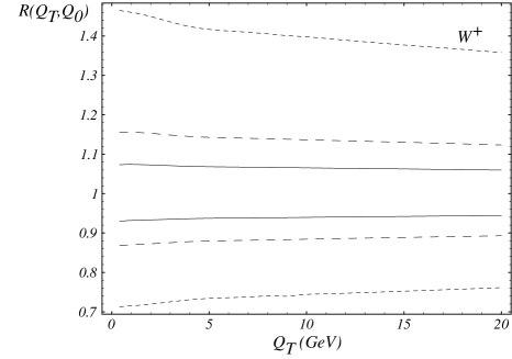
Figure 3.6: The ratio $R(Q_{T},Q_{0})$, with $y_{0}=0$, for $W^{+}$ and $Z^{0}$ bosons as a function of $Q_{T}$. For $W^{+}$, solid lines are: $Q_{0}=78$ GeV (upper) and 82 GeV (lower), dashed: $Q_{0}=76$ GeV (upper) and 84 GeV (lower), dotted: $Q_{0}=70$ GeV (upper) and 90 GeV (lower). For $Z^{0}$ bosons, solid lines: $Q_{0}=88$ GeV (upper) and 92 GeV (lower), dashed: $Q_{0}=86$ GeV (upper) and 94 GeV (lower), dotted: $Q_{0}=80$ GeV (upper) and 100 GeV (lower).

Similarly, we define the ratio

$$R(Q_{T},y_{0})={\frac{\left.\displaystyle\frac{d\sigma}{dQ^{2}dQ_{T}^{2}dy}\right|_{Q=M_{V},y=y_{0}}}{\left.\displaystyle\frac{d\sigma}{dQ^{2}dQ_{T}^{2}dy}\right|_{Q=M_{V},y=0}}},$$

to study the $Q_{T}$ shape variation as a function of the vector boson rapidity. Our results are shown in Fig. 3.7. Unlike the ratio $R(Q_{T},Q_{0})$ shown in Fig. 3.6, the distributions of $R(Q_{T},y_{0})$ for the $W^{\pm}$ and $Z^{0}$ bosons are clearly different for any value of the rapidity $y_{0}$.

To utilize the information on the transverse momentum of the $W^{+}$ boson in Monte Carlo simulations to reconstruct the mass of the $W^{+}$ boson, it was suggested in Ref. [82] to predict $Q_{T}(W^{+})$ distribution from the measured $Q_{T}(Z^{0})$ distribution and the calculated ratio of $Q_{T}(W^{+})$ and $Q_{T}(Z^{0})$ predicted by the resummation calculations [45, 66], in which the vector boson is assumed to be on its mass-shell. Unfortunately, this idea will not work with a good precision because, as clearly shown in Fig. 3.7, the ratio of the $W^{+}$ and $Z^{0}$ transverse momentum distributions depends on the rapidities of the vector bosons. Since the rapidity of the $W^{+}$ boson cannot be accurately reconstructed without knowing the longitudinal momentum (along the beam pipe direction) of the neutrino, which is in the form of missing energy carried away by the neutrino, this dependence cannot be incorporated in data analysis and the above ansatz cannot be realized in practice for a precision measurement of $M_{W}$. Only the Monte Carlo implementation of the exact matrix element calculation (included in ResBos) can correctly predict the distributions of the decay leptons, such as the transverse mass of the $W^{\pm}$ boson, and the transverse momentum of the charged lepton, so that they can be directly compared with experimental data to extract the value of $M_{W}$. We comment on these results later in this section.

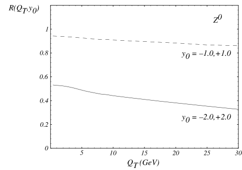
Figure 3.7: The ratio $R(Q_{T},y_{0})$, with $Q_{0}=M_{V}$, for $W^{+}$ and $Z^{0}$ bosons as a function of $Q_{T}$.

Another way to compare the results of the resummed and the NLO calculations is given by the distributions of $\sigma(Q_{T}>Q_{T}^{\min})/\sigma_{Total}$, as shown in Fig. 3.8. We defined the ratio as

$$R_{CSS}\equiv\frac{\sigma(Q_{T}>Q_{T}^{\min})}{\sigma_{Total}}=\frac{1}{\sigma_{Total}}\int_{Q_{T}^{\min}}^{Q_{T}^{\max}}dQ_{T}\;\frac{d\sigma(h_{1}h_{2}\rightarrow V)}{dQ_{T}},$$

where $Q_{T}^{\max}$ is the largest $Q_{T}$ allowed by the phase space. In the NLO calculation, $\sigma(Q_{T}>Q_{T}^{\min})$ grows without bound near $Q_{T}^{\min}=0$, as the result of the singular behavior $1/Q_{T}^{2}$ in the matrix element. The NLO curve runs well under the resummed one in the 2 GeV $<Q_{T}^{\min}<$ 30 GeV region, and the $Q_{T}$ distributions from the NLO and the resummed calculations have different shapes even in the region where $Q_{T}$ is of the order 15 GeV.

With large number of fully reconstructed $Z^{0}$ events at the Tevatron, one should be able to use data to discriminate these two theory calculations. In view of this result it is not surprising that the DØ  analysis of the $\alpha_{s}$ measurement [83] based on the measurement of $\sigma(W+1\;jet)/\sigma(W+0\;jet)$ does not support the NLO calculation in which the effects of the multiple gluon radiation are not included. We expect that if this measurement was performed by demanding the transverse momentum of the jet to be larger than about 50 GeV, at which scale the resummed and the NLO distributions in Fig. 3.2 cross, the NLO calculation would adequately describe the data.

Figure 3.8: The ratio $R_{CSS}$ as a function of $Q_{T}^{\min}$ for $W^{+}$ and $Z^{0}$ bosons. The fixed order (${\cal O}(\alpha_{s})$ short dashed, ${\cal O}(\alpha_{s}^{2})$ dashed) curves are ill-defined in the low $Q_{T}$ region. The resummed (solid) curves are calculated for $g_{2}$ = 0.38 (low), 0.58 (middle) and 0.68 (high) GeV² values.

To show that for $Q_{T}$ below 30 GeV, the QCD multiple soft gluon radiation is important to explain the DØ  data [83], we also include in Fig. 3.8 the prediction for the $Q_{T}$ distribution at the order of $\alpha^{2}_{S}$. As shown in the figure, the $\alpha^{2}_{S}$ curve is closer to the resummed curve which proves that for this range of $Q_{T}$ the soft gluon effect included in the $\alpha^{2}_{S}$ calculation is important for predicting the vector boson $Q_{T}$ distribution. In other words, in this range of $Q_{T}$, it is more likely that soft gluons accompany the $W^{\pm}$ boson than just a single hard jet associated with the vector boson production. For large $Q_{T}$, it becomes more likely to have hard jet(s) produced with the vector boson.

Measuring $R_{CSS}$ in the low $Q_{T}$ region (for $Q_{T}{\ \lower-1.2pt\vbox{\hbox{\hbox to0.0pt{$<$\hss}\lower 5.0pt\vbox{\hbox{$\sim$}}}}\ }Q/2$) provides a stringent test of the dynamics of the multiple soft gluon radiation predicted by the QCD theory. The same measurement of $R_{CSS}$ can also provide information about some part of the non-perturbative physics associated with the initial state hadrons. As shown in Fig. 3.9 and in Ref. [73], the effect of the non-perturbative physics on the $Q_{T}$ distributions of the $W^{\pm}$ and $Z^{0}$ bosons produced at the Tevatron is important for $Q_{T}$ less than about 10 GeV. This is evident by observing that different parametrizations of the non-perturbative functions do not change the $Q_{T}$ distribution for $Q_{T}>10$ GeV, although they do dramatically change the shape of $Q_{T}$ for $Q_{T}<10$ GeV. Since for $W^{\pm}$ and $Z^{0}$ production, the $\ln(Q^{2}/Q^{2}_{0})$ term is large, the non-perturbative function, as defined in Eq. (2.11), is dominated by the $F_{1}(b)$ term (or the $g_{2}$ parameter) which is supposed to be universal for all Drell-Yan type processes and related to the physics of the renormalon [71]. Hence, the measurement of $R_{CSS}$ cannot only be used to test the dynamics of the QCD multiple soft gluon radiation, in the $10\,{\rm GeV}\,<Q_{T}<40$ GeV region, but may also be used to probe this part of non-perturbative physics for $Q_{T}<10$ GeV. It is therefore important to measure $R_{CSS}$ at the Tevatron. With a large sample of $Z^{0}$ data at Run 2, it is possible to determine the dominant non-perturbative function which can then be used to calculate the $W^{\pm}$ boson $Q_{T}$ distribution to improve the accuracy of the $M_{W}$ and the charged lepton rapidity asymmetry measurements.

Figure 3.9: Transverse momentum distributions of $W^{+}$ and $Z^{0}$ bosons calculated with low (long dash, $g_{2}$ = 0.38 GeV²), nominal (solid, $g_{2}$ = 0.58 GeV²) and high (short dash, $g_{2}$ = 0.68 GeV²) $g_{2}$ non-perturbative parameter values. The low and high excursions in $g_{2}$ are the present one standard deviations from the nominal value in the Ladinsky-Yuan parametrization.

The transverse momentum distribution of $W^{\pm}$ bosons within a modified CSS formalism was also calculated by in Ref. [84]. The conclusions and results, when they overlap, agree with ours.

3.1.2 Vector Boson Longitudinal Distributions

The resummation of the logs involving the transverse momentum of the vector boson does not directly affect the shape of the longitudinal distributions of the vector bosons. A good example of this is the distribution of the longitudinal momentum of the $Z^{0}$ boson which can be measured at the Tevatron with high precision, and can be used to extract information on the parton distributions. It is customary to plot the rescaled quantity $x_{F}=2q^{3}/\sqrt{S}$, where $q^{3}=\sinh(y)\sqrt{Q^{2}+Q_{T}^{2}}$ is the longitudinal momentum of the $Z^{0}$ boson measured in the laboratory frame. In Fig. 3.10, we plot the distributions predicted in the resummed and the NLO calculations. As shown, their total event rates are different in the presence of kinematic cuts. (Although they are the same if no kinematic cuts imposed.) This conclusion is similar to that of the $y^{\ell}$ distributions, as discussed in Sections 3.1.3 and 3.2.1.

Figure 3.10: Longitudinal $x_{F}$ distributions of $Z^{0}$ bosons produced at the Tevatron. The NLO (dashed) curves overestimate the rate compared to the resummed (solid) ones, because kinematic cuts enhance the low $Q_{T}$ region where the NLO and resummed distributions are qualitatively different. Without cuts, the NLO and the resummed $x_{F}$ distributions are the same.

Without any kinematic cuts, the vector boson rapidity distributions are also the same in the resummed and the NLO calculations. This is so because when calculating the $y$ distribution the transverse momentum $Q_{T}$ is integrated out so that the integral has the same value in the NLO and the resummed calculations. On the other hand, experimental cuts on the final state leptons restrict the phase space, so the difference between the NLO and the resummed $Q_{T}$ distributions affects the vector boson rapidity distributions. This shape difference is very small at the vector boson level, as shown in Fig. 3.11.

Figure 3.11: Rapidity distributions (resummed: solid, NLO: dashed) of $Z^{0}$ bosons produced at the Tevatron with the kinematic cuts given in the text.

3.1.3 The Total Cross Section

Before we compare the distributions of the decay leptons, we examine the question whether or not the $Q_{T}$ resummation formalism changes the prediction for the total cross section. In Ref. [85] it was shown that in the AEGM formalism, which differs from the CSS formalism, the ${\cal O}(\alpha_{s})$ total cross section is obtained after integrating their resummation formula over the whole range of the phase space.

In the CSS formalism, without including the $C$ and $Y$ functions, the fully integrated resummed result recovers the ${\cal O}(\alpha_{s}^{0})$ cross section, provided that $Q_{T}$ is integrated from zero to $Q$. This can be easily verified by expanding the resummation formula up to ${\cal O}(\alpha_{S})$, dropping the $C^{(1)}$ and the $Y$ pieces (which are of order ${\cal O}(\alpha_{s})$), and integrating over the lepton variables. It yields

$$\int_{0}^{P_{T}^{2}}dQ_{T}^{2}\;\frac{d\sigma}{dQ^{2}dydQ_{T}^{2}}=\frac{\sigma_{0}}{S}\delta(Q^{2}-M_{V}^{2})$$ (3.1)

$$\ \ \ \ \ \times\left\{\left(1-\frac{\alpha_{s}(Q)}{\pi}\left[\frac{1}{2}A^{(1)}\ln^{2}\left(\frac{Q^{2}}{P_{T}^{2}}\right)+B^{(1)}\ln\left(\frac{Q^{2}}{P_{T}^{2}}\right)\right]\right)\right.$$

$$~{}~{}~{}~{}~{}~{}~{}~{}~{}~{}\left.\times\;f_{j/h_{1}}(x_{1},Q^{2})\;f_{\overline{k}/h_{2}}(x_{2},Q^{2})\right.$$

$$\ \ \ \ \ -\frac{\alpha_{s}(Q)}{2\pi}\ln\left(\frac{Q^{2}}{P_{T}^{2}}\right)\left[\left(P_{j\leftarrow a}\otimes f_{a/h_{1}}\right)(x_{1},Q^{2})\;f_{\overline{k}/h_{2}}(x_{2},Q^{2})\right.$$

$$~{}~{}~{}~{}~{}~{}~{}~{}~{}~{}~{}~{}~{}~{}~{}~{}~{}~{}~{}~{}~{}~{}~{}~{}\left.\left.+\;f_{j/h_{1}}(x_{1},Q^{2})\left(P_{\overline{k}\leftarrow b}\otimes f_{b/h_{2}}\right)(x_{2},Q^{2})\right]+j\leftrightarrow\overline{k}\right\},$$

where $P_{T}$ is the upper limit of the $Q_{T}$ integral and we fixed the mass of the vector boson for simplicity. To derive the above result we have used the canonical set of the $C_{i}$ ($i=1,2,3$) coefficients (cf. Section 2.2.4). When the upper limit $P_{T}$ is taken to be $Q$, all the logs in the above equation vanish and Eq. (3.1) reproduces the Born level (${\cal O}(\alpha_{s}^{0})$) cross section. Similar conclusion holds for higher order terms from the expansion of the resummed piece when $C$ and $Y$ are not included. This is evident because the singular pieces from the expansion are given by

$$\left.\frac{d\sigma}{dQ_{T}^{2}}\right|_{singular}=\frac{1}{Q_{T}^{2}}\sum_{n=1}^{\infty}\sum_{m=0}^{2n-1}{}_{n}v_{m}\alpha_{s}^{n}\ln^{m}\left(\frac{Q_{T}^{2}}{Q^{2}}\right)$$

The integral of these singular terms will be proportional to $\ln(Q^{2}/P_{T}^{2})$ raised to some power. Again, for $P_{T}=Q$ all the logs vanish and the tree level result is obtained.

Including $C^{(1)}$ and the $Y$ contribution changes the above conclusion and leads to a different total cross section, because $C^{(1)}$ contains the hard part virtual corrections and $Y$ contains the hard gluon radiation. Combining the resummed (1,1,1) and the fixed order ${\cal O}(\alpha_{s})$ distributions, the above described matching prescription provides us with an ${\cal O}(\alpha_{s})$ resummed total cross section with an error of ${\cal O}(\alpha_{s}^{2})$, as shown in Ref. [66]. In practice this translates into less than a percent deviation between the resummed ${\cal O}(\alpha_{s})$ total cross section and the inclusive NLO (${\cal O}(\alpha_{s})$) calculation. This can be understood from the earlier discussion that if the matching were done at $Q_{T}$ equal to $Q$, then the total cross section calculated from the CSS resummation formalism should be the same as that predicted by the NLO calculation, provided that $C^{(1)}$ and $Y^{(1)}$ are included. However, this matching prescription would not result in a smooth curve for the $Q_{T}$ distribution at $Q_{T}=Q$. The matching procedure described above causes a small (about a percent) difference between the ${\cal O}(\alpha_{s})$ resummed and the NLO total cross sections. This difference indicates the typical size of the higher order corrections not included in the NLO total cross section calculation.

The total cross section predicted from the various theory calculations are listed in Table 3.2.

	$E_{cm}$	Fixed Order		Resummed			Experiment
	(TeV)	${\cal O}(\alpha_{s}^{0})$	${{\cal O}(\alpha_{s})}$	(1,1,1)	(2,1,1)	(2,1,2)	(Ref. [86])
				$\oplus~{}{\cal O}(\alpha_{s})$	$\oplus~{}{\cal O}(\alpha_{s})$	$\oplus~{}{\cal O}(\alpha_{s}^{2})$
W+	1.8	8.81	11.1	11.3	11.3	11.4	11.5 $\pm$ 0.7
W+	2.0	9.71	12.5	12.6	12.6	12.7
Z0	1.8	5.23	6.69	6.79	6.79	6.82	6.86 $\pm$ 0.36
Z0	2.0	6.11	7.47	7.52	7.52	7.57

Table 3.2: Total cross sections of $p{\bar{p}}\rightarrow(W^{+}{\rm or}~{}Z^{0})X$ at the present and upgraded Tevatron, calculated in different prescriptions, in units of nb. The finite order total cross section results are based on the calculations in Ref. [85]. The ${\cal O}(\alpha_{s}^{2})$ results were obtained from Ref. [65]. The “$\oplus$” signs refer to the matching prescription discussed in the text.

As shown in Table 3.2, as far as the total rate is concerned, there is hardly any observable difference between the predicted results from the resummed (2,1,1) matched to the fixed order perturbative ${\cal O}(\alpha_{s})$ and the resummed (2,1,2) matched to the fixed order perturbative ${\cal O}(\alpha_{s}^{2})$, although the latter gives a smoother $Q_{T}$ curve, as shown in Fig. 3.2.

Kinematic cuts affect the total cross section in a subtle manner. It is obvious from our matching prescription that the resummed ${\cal O}(\alpha_{S}^{2})$ and the fixed order ${\cal O}(\alpha_{s})$ curves in Fig. 3.2 will never cross in the high $Q_{T}$ region. On the other hand, the resummed ${\cal O}(\alpha_{s}^{2})$ total cross section is about the same as the fixed order ${\cal O}(\alpha_{s})$ cross section when integrating $Q_{T}$ from 0 to $Q$. These two facts imply that when kinematic cuts are made on the $Q_{T}$ distribution with $Q_{T}<Q$, we will obtain a higher total cross section in the fixed order ${\cal O}(\alpha_{s})$ than in the resummed ${\cal O}(\alpha_{s}^{2})$ calculation. In this Chapter we follow the CDF cuts (for the $W^{+}$ boson mass analysis) and demand $Q_{T}<30$ GeV [87]. Consequently, in many of our figures, to be shown below, the fixed order ${\cal O}(\alpha_{s})$ curves give about 3% higher total cross section than the resummed ones.

3.2 Lepton Distributions

3.2.1 Lepton Charge Asymmetry

The CDF lepton charge asymmetry measurement [88] played a crucial role in constraining the slope of the $u/d$ ratio in recent parton distribution functions. It was shown that one of the largest theoretical uncertainty in the $W^{\pm}$ mass measurement comes from the parton distributions [89], and the lepton charge asymmetry was shown to be correlated with the transverse mass distribution [90]. Among others, the lepton charge asymmetry is studied to decrease the errors in the measurement of $M_{W}$ coming from the parton distributions. Here we investigate the effect of the resummation on the lepton rapidity distribution, although it is not one of those observables which are most sensitive to the $Q_{T}$ resummation, i.e. to the effect of multiple soft gluon radiation.

The definition of the charge asymmetry is

$$A(y)=\frac{\displaystyle\frac{d\sigma}{dy_{+}}-\frac{d\sigma}{dy_{-}}}{\displaystyle\frac{d\sigma}{dy_{+}}+\frac{d\sigma}{dy_{-}}},$$

where $y_{+}$ ($y_{-}$) is the rapidity of the positively (negatively) charged particle (either vector boson or decay lepton). Assuming CP invariance, the following relation holds:

$${\frac{d\sigma}{dy_{+}}}(y)={\frac{d\sigma}{dy_{-}}}(-y).$$

Hence, the charge asymmetry is frequently written as

$$A(y)=\frac{\displaystyle\frac{d\sigma}{dy}(y>0)-\frac{d\sigma}{dy}(y<0)}{\displaystyle\frac{d\sigma}{dy}(y>0)+\frac{d\sigma}{dy}(y<0)}.$$

For the charge asymmetry of the vector boson ($W^{\pm}$) or the charged decay lepton ($\ell^{\pm}$), the fixed order and the resummed ${\cal O}(\alpha_{s})$ [or ${\cal O}(\alpha_{s}^{2})$] results are the same, provided that there are no kinematic cuts imposed. This is because the shape difference in the vector boson transverse momentum has been integrated out and the total cross sections are the same up to higher order corrections in $\alpha_{s}$. In Fig. 3.12(a) we show the lepton charge asymmetry without cuts for CTEQ4M PDF. The NLO and the resummed curves overlap, although they differ from the ${\cal O}(\alpha_{s}^{0})$ prediction.

Figure 3.12: Lepton charge asymmetry distributions. (a) Without any kinematic cuts, the NLO (long dashed) and the resummed ${\cal O}(\alpha_{s})$ (solid) curves overlap and the LO (short dashed) curve differs somewhat from them. (b) With cuts ($Q_{T}<30$ GeV, $p_{T}^{e,\nu}>25$ GeV), the effect of the different $Q_{T}$ distributions renders the lepton rapidity asymmetry distributions different. The two resummed curves calculated with $g_{2}$ = 0.58 and 0.78 GeV² cannot be distinguished on this plot.

On the other hand, when kinematic cuts are applied to the decay leptons, the rapidity distributions of the vector bosons or the leptons in the fixed order and the resummed calculations are different. Restriction of the phase space implies that only part of the vector boson transverse momentum distribution is sampled. The difference in the resummed and the fixed order $Q_{T}$ distributions will prevail as a difference in the rapidity distributions of the charged lepton. We can view this phenomenon in a different (a Monte Carlo) way. In the rest frame of the $W^{\pm}$, the decay kinematics is the same, whether it is calculated up to ${\cal O}(\alpha_{s})$ or within the resummation formalism. On the other hand, the $W^{\pm}$ rest frame is different for each individual Monte Carlo event depending on the order of the calculation. This difference is caused by the fact that the $Q_{T}$ distribution of the $W^{\pm}$ is different in the ${\cal O}(\alpha_{s})$ and the resummed calculations, and the kinematic cuts select different events in these two cases. Hence, even though the $Q_{T}$ distribution of the $W^{\pm}$ is integrated out, when calculating the lepton rapidity distribution, we obtain slightly different predictions in the two calculations. The difference is larger for larger $|y^{\ell}|$, being closer to the edge of the phase space, because the soft gluon radiation gives high corrections there and this effect up to all order in $\alpha_{s}$ is contained in the resummed but only up to order of $\alpha_{s}$ in the NLO calculation. Because the rapidity of the lepton and that of the vector boson are highly correlated, large rapidity leptons mostly come from large rapidity vector bosons. Also, a vector boson with large rapidity tends to have low transverse momentum, because the available phase space is limited to low $Q_{T}$ for a $W^{\pm}$ boson with large $|y|$. Hence, the difference in the low $Q_{T}$ distributions of the NLO and the resummed calculations yields the difference in the $y^{\ell}$ distribution for leptons with high rapidities.

Asymmetry distributions of the charged lepton with cuts using the CTEQ4M PDF are shown in Fig. 3.12(b). The applied kinematic cuts are: $Q_{T}<30$ GeV, $p_{T}^{e^{+},\nu}>25$. These are the cuts that CDF used when extracted the lepton rapidity distribution from their data [88]. We have checked that the ResBos fixed order ${\cal O}(\alpha_{s})$ curve agrees well with the DYRAD [80] result. As anticipated, the ${\cal O}(\alpha_{s}^{0})$, ${\cal O}(\alpha_{s})$ and resummed results deviate at higher rapidities ($|y^{e}|>1.5$). The deviation between the NLO and the resummed curves indicates that to extract information on the PDF in the large rapidity region, the resummed calculation, in principle, has to be used if the precision of the data is high enough to distinguish these predictions. Fig. 3.12(b) also shows the negligible dependence of the resummed curves on the non-perturbative parameter $g_{2}$. We plot the result of the resummed calculations with the nominal $g_{2}$ = 0.58 GeV², and with $g_{2}$ = 0.78 GeV² which is two standard deviations higher. The deviation between these two curves (which is hardly observable on the figure) is much smaller than the deviation between the resummed and the NLO ones.

There is yet another reason why the lepton charge asymmetry can be reliably predicted only by the resummed calculation. When calculating the lepton distributions in a numerical ${\cal O}(\alpha_{s})$ code, one has to artificially divide the vector boson phase space into hard and soft regions, depending on – for example – the energy or the $Q_{T}$ of the emitted gluon (e.g. $q\overline{q}\rightarrow W+\;$hard or soft gluon). The observables calculated with this phase space slicing technique acquire a dependence on the scale which separates the hard from the soft regions. For example, when the phase space is divided by the $Q_{T}$ separation, the dependence of the asymmetry on the scale $Q_{T}^{Sep}$ can be comparable to the difference in the ${\cal O}(\alpha_{s})$ and the resummed results. This means that there is no definite prediction from the NLO calculation for the lepton rapidity distribution. Only the resummed calculation can give an unambiguous prediction for the lepton charge asymmetry.

Before closing this section, we also note that although in the lepton asymmetry distribution the NLO and resummed results are about the same for $|y^{e^{+}}|<1$, it does not imply that the rapidity distributions of the leptons predicted by those two theory models are the same. As shown in Fig. 3.13, this difference can in principle be observable with a large statistics data sample and a good knowledge of the luminosity of the colliding beams.

Figure 3.13: Distributions of positron rapidities from the decays of $W^{+}$’s produced at the Tevatron, predicted by the resummed (solid) and the NLO (dashed) calculations with the same kinematic cuts as for the asymmetry plot.

3.2.2 Transverse Mass Distribution

Since the invariant mass of the $W^{\pm}$ boson cannot be reconstructed without knowing the longitudinal momentum of the neutrino, one has to find a quantity that allows an indirect determination of the mass of the $W^{\pm}$ boson. In the discovery stage of the $W^{\pm}$ bosons at the CERN ${\rm Sp\overline{p}S}$ collider, the mass and width were measured using the transverse mass distribution of the charged lepton-neutrino pair from the $W^{\pm}$ boson decay. Ever since the early eighties, the transverse mass distribution, $m_{T}=\sqrt{2p_{T}^{e}p_{T}^{\nu}(1-\cos\Delta\phi_{e\nu})}$, has been known as the best measurable for the extraction of both $M_{W}$ and $\Gamma_{W}$, for it is insensitive to the transverse momentum of the $W^{\pm}$ boson. The effect of the non-vanishing vector boson transverse momentum on the $m_{T}$ distribution was analyzed  [91, 92] well before the $Q_{T}$ distribution of the $W^{\pm}$ boson was correctly calculated by taking into account the multiple soft gluon radiation. Giving an average transverse boost to the vector boson, the authors of Ref. [91] concluded that for the fictive case of $\Gamma_{W}$ = 0, the end points of the transverse mass distribution are fixed at zero: $d\sigma/dm_{T}^{2}(m_{T}^{2}=0)=d\sigma/dm_{T}^{2}(m_{T}^{2}=M_{W}^{2})=0$. The sensitivity of the $m_{T}$ shape to a non-zero $Q_{T}$ is in the order of $\left\langle(Q_{T}/M_{W})^{2}\right\rangle\approx$1% without affecting the end points of the $m_{T}$ distribution. Including the effect of the finite width of the $W^{\pm}$ boson, the authors in Ref. [92] showed that the shape and the location of the Jacobian peak are not sensitive to the $Q_{T}$ of the $W^{\pm}$ boson either. The non-vanishing transverse momentum of the $W^{\pm}$ boson only significantly modifies the $m_{T}$ distribution around $m_{T}=0$.

Our results confirm that the shape of the Jacobian peak is quite insensitive to the order of the calculation. We show the NLO and the resummed transverse mass distributions in Fig. 3.14 for $W^{\pm}$ bosons produced at the Tevatron with the kinematic cuts: $Q_{T}<30$ GeV, $p_{T}^{e^{+},\nu}>25$ GeV and $|y^{e^{+}}|<3.0$. Fig. 3.14(a) covers the full (experimentally interesting) $m_{T}$ range while Fig. 3.14(b) focuses on the $m_{T}$ range which contains most of the information about the $W^{\pm}$ mass. There is little visible difference between the $shapes$ of the NLO and the resummed $m_{T}$ distributions. On the other hand, the right shoulder of the curve appears to be “shifted” by about 50 MeV, because, as noted in Section 3.1.3, the total cross sections are different after the above cuts imposed in the NLO and the resummed calculations. At Run 2 of the Tevatron, with large integrated luminosity ($\sim 2~{}{\rm fb}^{-1}$), the goal is to extract the $W^{\pm}$ boson mass with a precision of 30-50 MeV from the $m_{T}$ distribution [89]. Since $M_{W}$ is sensitive to the position of the Jacobian peak [92], the high precision measurement of the $W^{\pm}$ mass has to rely on the resummed calculations.

Figure 3.14: Transverse mass distribution for $W^{+}$ production and decay at the 1.8 TeV Tevatron.

The extraction of $M_{W}$ from the transverse mass distribution has some drawbacks. The reconstruction of the transverse momentum $p_{T}^{\nu}$ of the neutrino involves the measurement of the underlying event transverse momentum: $\vec{p}_{T}^{~{}\nu}=-\vec{p}_{T}^{~{}\ell}-\vec{p}_{T}^{~{}recoil}-\vec{p}_{T}^{~{}underlying~{}event}$. This resolution degrades by the number of interactions per crossing ($N_{I_{c}}$) [89]. With a high luminosity ($\sim 100\,{\rm fb}^{-1}$) at the 2 TeV Tevatron (TEV33) [93], $N_{I_{c}}$ can be as large as 10, so that the Jacobian peak is badly smeared. This will lead to a large uncertainty in the measurement of $M_{W}$. For this reason the systematic precision of the $m_{T}$ reconstruction will be less at the high luminosity Tevatron, and an $M_{W}$ measurement that relies on the lepton transverse momentum distribution alone could be more promising. We discuss this further in the next section.

The theoretical limitation on the $M_{W}$ measurement using the $m_{T}$ distribution comes from the dependence on the non-perturbative sector, i.e. from the PDF’s and the non-perturbative parameters in the resummed formalism. Assuming the PDF’s and these non-perturbative parameters to be independent variables, the uncertainties introduced are estimated to be less than 50 MeV and 10 MeV, respectively, at the TEV33 [81, 94]. It is clear that the main theoretical uncertainty comes from the PDF’s. As to the uncertainty due to the non-perturbative parameters (e.g. $g_{2}$) in the CSS resummation formalism, it can be greatly reduced by carefully study the $Q_{T}$ distribution of the $Z^{0}$ boson which is expected to be copiously produced at Run 2 and beyond.

The $M_{W}$ measurement at the LHC may also be promising. Both ATLAS and CMS detectors are well optimized for measuring the leptons and the missing $E_{T}$ [94]. The cross section of the $W^{+}$ boson production is about four times larger than that at the Tevatron, and in one year of running with 20 fb^-1 luminosity yields a few times $10^{7}$ $W\rightarrow\ell\nu$ events after imposing similar cuts to those made at the Tevatron. Since the number of interactions per crossing may be significantly lower (in average $N_{I_{c}}$ = 2) at the same or higher luminosity than that at the TEV33 [94], the Jacobian peak in the $m_{T}$ distribution will be less smeared at the LHC than at the TEV33. Furthermore, the non-perturbative effects are relatively smaller at the LHC because the perturbative Sudakov factor dominates. On the other hand, the probed region of the PDF’s at the LHC has a lower value of the average $x~{}(\sim 10^{-3})$ than that at the Tevatron $(\sim 10^{-2})$, hence the uncertainty from the PDF’s might be somewhat larger. A more detailed study of this subject is desirable.

3.2.3 Lepton Transverse Momentum

Due to the limitations mentioned above, the transverse mass method may not be the only and the most promising way for the precision measurement of $M_{W}$ at some future hadron colliders. As discussed above, the observable $m_{T}$ was used because of its insensitivity to the high order QCD corrections. In contrast, the lepton transverse momentum ($p_{T}^{\ell}$) distribution receives a large, ${\cal O}\left(\left\langle Q_{T}/M_{W}\right\rangle\right)\sim 10\%$, perturbative QCD correction at the order $\alpha_{s}$, as compared to the Born process. With the resummed results in hand it becomes possible to calculate the $p_{T}^{\ell}$ distribution precisely within the perturbative framework, and to extract the $W^{\pm}$ mass straightly from the transverse momentum distributions of the decay leptons.

Just like in the $m_{T}$ distribution, the mass of the $W^{\pm}$ boson is mainly determined by the shape of the distribution near the Jacobian peak. The location of the maximum of the peak is directly related to the $W^{\pm}$ boson mass, while the theoretical width of the peak varies with its decay width $\Gamma_{W}$. Since the Jacobian peak is modified by effects of both $Q_{T}$ and $\Gamma_{W}$, it is important to take into account both of these effects correctly. In our calculation (and in ResBos) we have properly included both effects.

The effect of resummation on the transverse momentum distribution of the charged lepton from $W^{+}$ and $Z^{0}$ decays is shown in Fig. 3.15. The NLO and the resummed distributions differ a great amount even without imposing any kinematic cuts. The clear and sharp Jacobian peak of the NLO distribution is strongly smeared by the finite transverse momentum of the vector boson introduced by multiple gluon radiation. This higher order effect cannot be correctly calculated in any finite order of the perturbation theory and the resummation formalism has to be used.

Figure 3.15: Transverse momentum distributions of $p_{T}^{e^{+}}$ from $W^{+}$ and $Z^{0}$ decays for the NLO (dashed) and the resummed ${\cal O}(\alpha_{s})$ (solid) calculations. Resumming the initial state multiple soft-gluon emission has the typical effect of smoothening and broadening the Jacobian peak (at $p_{T}^{e^{+}}=M_{V}/2$). The CDF cuts are imposed on the $W^{+}$ distributions, but there are no cuts on the $Z^{0}$ distributions.

One of the advantages of using the $p_{T}^{\ell}$ distribution to determine $M_{W}$ is that there is no need to reconstruct the $p_{T}^{\nu}$ distribution which potentially limits the precision of the $m_{T}$ method. From the theoretical side, the limitation is in the knowledge of the non-perturbative sector. Studies at DØ  [95] show that the $p_{T}^{\ell}$ distribution is most sensitive to the PDF’s and the value of the non-perturbative parameter $g_{2}$. The $p_{T}^{\ell}$ distribution is more sensitive to the PDF choice, than the $m_{T}$ distribution is. The uncertainty in the PDF causes an uncertainty in $M_{W}$ of about 150 MeV, which is about three times as large as that using the $m_{T}$ method [95]. A 0.1 GeV² uncertainty in $g_{2}$ leads to about $\Delta M_{W}=30$ MeV uncertainty from the $p_{T}^{\ell}$ fit, which is about five times worse than that from the $m_{T}$ measurement [95]. Therefore, to improve the $M_{W}$ measurement, it is necessary to include the $Z^{0}$ data sample at the high luminosity Tevatron to refit the $g_{i}$’s and obtain a tighter constrain on them from the $Q_{T}$ distribution of the $Z^{0}$ boson. The DØ  study showed that an accuracy of $\Delta g_{2}=0.01$ GeV² can be achieved with Run 2 and TeV33 data, which would contribute an error of $\Delta M_{W}<5$ MeV from the $p_{T}^{\ell}$ [95]. In this case the uncertainty coming from the PDF’s remains to be the major theoretical limitation. At the LHC, the $p_{T}^{\ell}$ distribution can be predicted with an even smaller theoretical error coming from the non-perturbative part, because at higher energies the perturbative Sudakov factor dominates over the non-perturbative function.

It was recently suggested to extract $M_{W}$ from the ratios of the transverse momenta of leptons produced in $W^{\pm}$ and $Z^{0}$ decay [96]. The theoretical advantage is that the non-perturbative uncertainties are decreased in such a ratio. On the other hand, it is not enough that the ratio of cross sections is calculated with small theoretical errors. For a precision extraction of the $W^{\pm}$ mass the theoretical calculation must be capable of reproducing the individually observed transverse momentum distributions themselves. The $W^{\pm}$ mass measurement requires a detailed event modeling, understanding of detector resolution, kinematical acceptance and efficiency effects, which are different for the $W^{\pm}$ and $Z^{0}$ events, as illustrated above. Therefore, the ratio of cross sections can only provide a useful check for the $W^{\pm}$ mass measurement.

For Drell-Yan events or lepton pairs from $Z^{0}$ decays, additional measurable quantities can be constructed from the lepton transverse momenta. They are the distributions in the balance of the transverse momenta $(\Delta{p}_{T}=|{\vec{p}}_{T}^{\,\ell_{1}}|-|{\vec{p}}_{T}^{\,{\bar{\ell}_{2}}}|)$ and the angular correlation of the two lepton momenta $({z=-\vec{p}}_{T}^{\,\ell_{1}}\cdot{\vec{p}}_{T}^{\,{\bar{\ell}_{2}}}/[\max(p_{T}^{\,\ell_{1}},p_{T}^{\,{\bar{\ell}_{2}}})]^{2})$. It is expected that these quantities are also sensitive to the effects of the multiple soft gluon radiation. These distributions are shown in Figure 3.16. As shown, the resummed distributions significantly differ from the NLO ones. In these, and the following figures for $Z^{0}$ decay distributions, it is understood that the following kinematic cuts are imposed: $Q_{T}^{Z^{0}}<30$ GeV, $p_{T}^{e^{+},e^{-}}>25$ GeV and $|y^{e^{+},e^{-}}|<3.0$, unless indicated otherwise.

Figure 3.16: Balance in transverse momentum $\Delta{p}_{T}=|{\vec{p}}_{T}^{\,\ell_{1}}|-|{\vec{p}}_{T}^{\,{\bar{\ell}_{2}}}|$ and angular correlation ${z=-\vec{p}}_{T}^{\,\ell_{1}}\cdot{\vec{p}}_{T}^{\,{\bar{\ell}_{2}}}/[\max(p_{T}^{\ell_{1}},p_{T}^{{\bar{\ell}_{2}}})]^{2}$ of the decay leptons from $Z^{0}$ bosons produced at the Tevatron.

3.2.4 Lepton Angular Correlations

Another observable that can serve to test the QCD theory beyond the fixed-order perturbative calculation is the difference in the azimuthal angles of the leptons $\ell_{1}$ and ${\bar{\ell}_{2}}$ from the decay of a vector boson $V$. In practice, this can be measured for $\gamma^{*}\rm{or}Z^{0}\rightarrow\ell_{1}{\bar{\ell}_{2}}$. We show in Fig. 3.17 the difference in the azimuthal angles of $e^{+}$ and $e^{-}$ ($\Delta\phi^{e^{+}e^{-}}$), measured in the laboratory frame for $Z^{0}\rightarrow e^{+}e^{-}$, calculated in the NLO and the resummed approaches. As indicated, the NLO result is ill-defined in the vicinity of $\Delta\phi\sim\pi$, where the multiple soft-gluon radiation has to be resummed to obtain physical predictions.

Figure 3.17: The correlation between the lepton azimuthal angles near the region $\Delta\phi\sim\pi$ for $p{\bar{p}}\rightarrow(Z^{0}\rightarrow e^{+}e^{-})X$. The resummed (solid) distribution gives the correct angular correlation of the lepton pair. The NLO (dashed lines) distribution near $\Delta\phi=\pi$ is ill-defined and depends on $Q_{T}^{Sep}$ (the scale for separating soft and hard gluons in the NLO calculation). The two NLO distributions were calculated with $Q_{T}^{Sep}=1.2$ GeV (long dash) and $Q_{T}^{Sep}=2.0$ GeV (short dash).

Another interesting angular variable is the lepton polar angle distribution $\cos\theta^{*\ell}$ in the Collins-Soper frame. It can be calculated for the $Z^{0}$ decay and used to extract $\sin^{2}\theta_{w}$ at the Tevatron [97]. The asymmetry in the polar angle distribution is essentially the same as the forward-backward asymmetry $A_{FB}$ measured at LEP. Since $A_{FB}$ depends on the invariant mass $Q$ and around the energy of the $Z^{0}$ peak $A_{FB}$ happens to be very small, the measurement is quite challenging. At the hadron collider, on the other hand, the invariant mass of the incoming partons is distributed over a range so the asymmetry is enhanced [98]. The potentials of the measurement deserve a separated study. In Fig. 3.18 we show the distributions of $\cos\theta^{*\ell}$ predicted from the NLO and the resummed results.

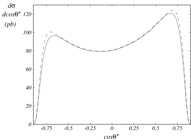
Figure 3.18: Distribution of the $e^{+}$ polar angle $\cos(\theta^{*})$ in the Collins-Soper frame from $Z^{0}$ decays at the Tevatron with cuts indicated in the text.

3.3 Conclusions

With a $100\,{\rm pb}^{-1}$ luminosity at the Tevatron, around $2\times 10^{6}$ $W^{\pm}$ and $6\times 10^{5}$ $Z^{0}$ bosons are produced, and the data sample will increase by a factor of 20 in the Run 2 era. In view of this large event rate, a careful study of the distributions of leptons from the decay of the vector bosons can provide a stringent test of the rich dynamics of the multiple soft gluon emission predicted by the QCD theory. Since an accurate determination of the mass of the $W^{\pm}$ boson and the test of parton distribution functions demand a highly precise knowledge of the kinematical acceptance and the detection efficiency of $W^{\pm}$ or $Z^{0}$ bosons, the effects of the multiple gluon radiation have to be taken into account. In this work, we have extended the formalism introduced by Collins, Soper and Sterman for calculating an on-shell vector boson to include the effects of the polarization and the decay width of the vector boson on the distributions of the decay leptons. Our resummation formalism can be applied to any vector boson $V$ where $V=\gamma^{*},\,W^{\pm},\,Z^{0},\,W^{\prime},\,Z^{\prime}$, etc., with either vector or axial-vector couplings to fermions (leptons or quarks). To illustrate how the multiple gluon radiation can affect the distributions of the decay leptons, we studied in detail various distributions for the production and the decay of the vector bosons at the Tevatron.

One of the methods to test the rich dynamics of the multiple soft gluon radiation predicted by the QCD theory is to measure the ratio $R_{CSS}\equiv\frac{\sigma(Q_{T}>Q_{T}^{\min})}{\sigma_{Total}}$ for the $W^{\pm}$ and $Z^{0}$ bosons. We found that, for the vector boson transverse momentum less than about 30 GeV, the difference between the resummed and the fixed order predictions (either at the $\alpha_{s}$ or $\alpha^{2}_{S}$ order) can be distinguished by experimental data. This suggests that in this kinematic region, the effects of the multiple soft gluon radiation are important, hence, the $Q_{T}$ distribution of the vector boson provides an ideal opportunity to test this aspect of the QCD dynamics. For $Q_{T}$ less than about 10 GeV, the distribution of $Q_{T}$ is largely determined by the non-perturbative sector of QCD. At the Tevatron this non-perturbative physics, when parametrized by Eq. (2.12) for $W^{\pm}$ and $Z^{0}$ production, is dominated by the parameter $g_{2}$ which was shown to be related to properties of the QCD vacuum [71]. Therefore, precisely measuring the $Q_{T}$ distribution of the vector boson in the low $Q_{T}$ region, e.g. from the ample $Z^{0}$ events, can advance our knowledge of the non-perturbative QCD physics.

Although the rapidity distributions of the leptons are not directly related to the transverse momentum of the vector boson, they are predicted to be different in the resummed and the fixed order calculations. This is because to compare the theoretical predictions with the experimental data, some kinematic cuts have to be imposed so that the signal events can be observed over the backgrounds. We showed that the difference is the largest when the rapidity of the lepton is near the boundary of the phase space (i.e. in the large rapidity region), and the difference diminishes when no kinematic cuts are imposed. When kinematic cuts are imposed another important difference between the results of the resummed and the NLO calculations is the prediction of the event rate. These two calculations predict different normalizations of various distributions. For example, the rapidity distributions of charged leptons ($y^{\ell^{\pm}}$) from the decays of $W^{\pm}$ bosons are different. They even differ in the central rapidity region in which the lepton charge asymmetry distributions are about the same (cf. Figs. 3.12 and 3.13). As noted in Ref. [90], with kinematic cuts, the measurement of $M_{W}$ is correlated to that of the rapidity and its asymmetry through the transverse momentum of the decay lepton. Since the resummed and the NLO results are different and the former includes the multiple soft gluon emission dynamics, the resummed calculation should be used for a precision measurement of $M_{W}$.

In addition to the rapidity distribution, we have also shown various distributions of the leptons which are either directly or indirectly related to the transverse momentum of the vector boson. For those which are directly related to the transverse momentum of the vector boson, such as the transverse momentum of the lepton and the azimuthal correlation of the leptons, the resummation formalism predicts significant differences from the fixed order perturbation calculations in some kinematic regions. The details were discussed in Section 3.2.

Figure 3.19: Transverse momentum distribution of virtual photons in $p{\bar{p}}\rightarrow\gamma^{*}\rightarrow e^{+}e^{-}$ events predicted by ResBos (solid curve) and ISAJET (histogram), calculated for the invariant mass range 30 GeV $<Q<$ 60 GeV at the 1.8 TeV Tevatron.

As noted in the Introduction, a full event generator, such as ISAJET, can predict a reasonable shape for various distributions because it contains the backward radiation algorithm [79], which effectively includes part of the Sudakov factor, i.e. effects of the multiple gluon radiation. However, the total event rate predicted by the full event generator is usually only accurate at the tree level, as the short distance part of the virtual corrections cannot yet be consistently implemented in this type of Monte Carlo program. To illustrate the effects of the high order corrections coming from the virtual corrections, which contribute to the Wilson coefficients $C$ in our resummation formalism, we showed in Fig. 3.19 the predicted distributions of the transverse momentum of the Drell-Yan pairs by ISAJET and by ResBos (our resummed calculation). In this figure we have rescaled the ISAJET prediction to have the same total rate as the ResBos result, so that the shape of the distributions can be directly compared. We restrict the invariant mass of the virtual photons $Q$ to be between 30 and 60 GeV without any kinematic cuts on the leptons. If additional kinematic cuts on the leptons are imposed, then the difference is expected to be enhanced, as discussed in Section 3.2.1. As clearly shown, with a large data sample in the future, it will be possible to experimentally distinguish between these two predictions, and, more interestingly, to start probing the non-perturbative sector of the QCD physics.

Chapter 4 Photon Pair Production In Hadronic Interactions

An increasing amount of prompt diphoton data is becoming available from the Tevatron collider and the fixed–target experiments at Fermilab [99, 100, 101]. After the upgrade of the Fermilab Tevatron the amount of the di-gauge boson data increases by a factor of 20, and the LHC by three order of magnitude. A comparison of the data to the calculation of the diphoton production rate and kinematic distributions provides a test of many aspects of perturbative quantum chromodynamics (pQCD). Furthermore, understanding the diphoton data is important for new physics searches. For example, diphoton production is an irreducible background to the light Higgs boson decay mode $h\to\gamma\gamma$. The next–to–leading order (NLO) cross section for the $p\bar{p}\to\gamma\gamma X$ process [102] was shown to describe well the invariant mass distribution of the diphoton pair after the leading order (LO) $gg\to\gamma\gamma$ contribution (from one–loop box diagrams) was included [103, 50]. However, to accurately describe the distribution of the transverse momentum of the photon pair and the kinematical correlation of the two photons, a calculation has to be performed that includes the effects of initial–state multiple soft–gluon emission.

In this Section, we extend the Collins–Soper–Sterman (CSS) soft gluon resummation formalism, to describe the production of photon pairs. This extension is similar to the formalism developed for describing the distribution of the leptons from vector boson decays in Chapter 2, because the final state of the diphoton process is also a color singlet state at LO. Initial–state multiple soft–gluon emission in the scattering subprocesses $q{\bar{q}},qg$ and $gg\to\gamma\gamma X$ is resummed by treating the photon pair $\gamma\gamma$ similarly to the Drell–Yan photon $\gamma^{*}$. In addition, there are contributions in which one of the final photons is produced through a long–distance fragmentation process. An example is $qg\to\gamma q$ followed by the fragmentation of the final state quark $q\to\gamma X$. An earlier study of soft–gluon resummation effects in photon pair production may be found in Ref. [104].

The results of the calculation are compared with CDF [99] and DØ  [100] data taken at the collider energy $\sqrt{S}=1.8$ TeV. A prediction for the production rate and kinematic distributions of the diphoton pair in proton–nucleon interactions at the fixed–target energy $\sqrt{S}=31.5$ GeV, appropriate for the E706 experiment at Fermilab [101], is also presented.

4.1 Diphoton Production at Fixed Order

Figure 4.1: Feynman diagrams representing the leading order and next–to–leading order contributions to photon pair production in hadron collisions. The shaded circles signify the production of long–distance fragmentation photons, which are described by the fragmentation function $D_{\gamma\leftarrow q}$.

The leading order (LO) subprocesses for diphoton production in hadron interactions are of order $\alpha_{em}^{2}$, where $\alpha_{em}$ denotes the electromagnetic coupling strength. There are three classes of LO partonic contributions to the reaction $h_{1}h_{2}\to\gamma\gamma X$, where $h_{1}$ and $h_{2}$ are hadrons, illustrated in Fig. (4.1a)–(4.1c). The first (4.1a) is the short–distance $q\bar{q}\to\gamma\gamma$ subprocess. The second (4.1b) is the convolution of the short–distance $qg\to\gamma q$ subprocess with the long–distance fragmentation of the final state quark $q\to\gamma X$. This is a LO contribution since the hard scattering is of order $\alpha_{em}\alpha_{s}$, while fragmentation is effectively of order $\alpha_{em}/\alpha_{s}$. Here, $\alpha_{s}$ denotes the QCD coupling strength. Class (4.1b) also includes the subprocess $q\bar{q}\to\gamma g$ convoluted with the fragmentation $g\to\gamma X$. Finally, there are LO contributions (4.1c) involving subprocesses like $qq\to qq$, where both final state quarks fragment $q\to\gamma X$. The transverse momenta of the photons are denoted $\vec{p}_{T_{1}}$ and $\vec{p}_{T_{2}}$, and the transverse momentum of the pair is $\vec{Q}_{T}=\vec{p}_{T_{1}}+\vec{p}_{T_{2}}$. In the absence of transverse momentum carried by the incident partons, the LO process (4.1a) provides $\vec{Q}_{T}=0$. With the added assumption of collinear final–state fragmentation, (4.1b) provides $\vec{Q}_{T}=\vec{p}_{T_{1}}+\vec{p}_{T_{2}}=(1-z)\vec{p}_{T_{1}}$, where photon 2 carries a fraction $z$ of the momentum of the final–state quark. Given a lower limit on the magnitude of the transverse momentum $p_{T}^{\gamma}$ of each photon, the total cross section at LO is finite.

The next–to–leading order (NLO) subprocesses for diphoton production are of order $\alpha_{em}^{2}\alpha_{s}$. One class of one–loop Feynman diagrams (4.1d) contributes by interfering with the tree level diagram (4.1a). Real gluon emission (4.1e) is also present at NLO. The subprocess $qg\to\gamma\gamma q$ contains a singular piece (4.1f) that renormalizes the lower order fragmentation (4.1b) and a piece (4.1g) that is free of final–state collinear singularities. Finally, subprocesses like $qq\to qq\gamma\gamma$ contain a regular piece involving photon emission convoluted with a fragmentation function (4.1h) and pieces that renormalize the double fragmentation process (4.1c). The regular 3–body final state contributions from (4.1e), (4.1f), and (4.1g) provide $\vec{Q}_{T}=-\vec{p}_{T_{j}}$, where $j$ represents the final–state quark or gluon. The full set of NLO contributions just described is free of final–state singularities, and the total integrated cross section at NLO is finite for a finite lower limit on each $p_{T}^{\gamma}$.

Higher order calculations in $\alpha_{s}$ improve the accuracy of predictions for total cross sections involving quarks or gluons when only one hard scale $Q$ is relevant. For $h_{1}h_{2}\to\gamma\gamma X$, this scale can be chosen proportional to the invariant mass of the photon pair, $Q=M_{\gamma\gamma}$, which is about equal to $2p_{T}^{\gamma}$ for two well separated photons in the central rapidity region. For kinematic distributions that depend on more than one scale, a NLO calculation may be less reliable. This is the case for the distribution of the transverse momentum of the photon pair, $Q_{T}=|\vec{Q}_{T}|$. Similarly to the Drell-Yan pair, at fixed $Q$, the behavior of the fixed order differential cross section for small $Q_{T}$ is

$$\lim_{Q_{T}\to 0}\frac{d\sigma}{dQ_{T}^{2}}=\sum_{n=0}^{\infty}\sum_{m=0}^{2n-1}\left(\frac{\alpha_{s}}{\pi}\right)^{n}\frac{{}_{n}v_{m}}{Q_{T}^{2}}\ln^{m}\left(\frac{Q^{2}}{Q_{T}^{2}}\right)+{\cal O}\left(\frac{1}{Q_{T}},\delta(Q_{T})\right),$$ (4.1)

where ${}_{n}v_{m}$ are calculable perturbatively. The structure of Eq. (4.1) indicates that the fixed order QCD prediction is reliable when $Q_{T}\simeq Q$, but becomes less reliable when $Q_{T}\ll Q$, where $\ln(Q^{2}/Q_{T}^{2})$ becomes large. In the region $Q_{T}\ll Q$, the photon pair is accompanied by soft and/or collinear gluon radiation. To calculate distributions like $\displaystyle\frac{d{\sigma}}{dQ_{T}^{2}}$ reliably in the region $Q_{T}\ll Q$, effects of multiple soft gluon emission must be taken into account. The contributions (4.1e) and (4.1g) exhibit singular behavior that can be tamed by resummation of the effects of initial–state multiple soft–gluon radiation to all orders in $\alpha_{s}$. Other contributions that do not become singular as $Q_{T}\to 0$ do not need to be treated in this manner. Fragmentation contributions like (4.1b) are found to be small in magnitude after isolation restrictions are imposed on the energy of the hadronic remnant from the fragmentation. Therefore, contributions like (4.1c) and (4.1h) are ignored in this work. Gluon fragmentation to a photon can be ignored, since its magnitude is small.

The subprocess $gg\to\gamma\gamma$, involving a quark box diagram, is of order $\alpha_{em}^{2}\alpha_{s}^{2}$. While formally of even higher order than the NLO contributions considered so far, this LO $gg$ contribution is enhanced by the size of the gluon parton distribution function. Consideration of the order $\alpha_{em}^{2}\alpha_{s}^{3}$ correction leads to resummation of the $gg$ subprocess in a manner analogous to the $q\bar{q}$ resummation.

4.2 Extension of the Resummation Formalism

4.2.1 The Resummation Formula

To improve upon the prediction of Eq. (4.1) for the region $Q_{T}\ll Q$, perturbation theory can be applied using an expansion parameter $\alpha_{s}^{m}\ln^{n}(Q^{2}/Q_{T}^{2})$, with $n=0,\ldots,2m-1,$ instead of $\alpha_{s}^{m}$. The terms $\alpha_{s}^{m}\ln^{n}(Q^{2}/Q_{T}^{2})$ represent the effects of soft gluon emission at order $\alpha_{s}^{m}$. Resummation of the singular part of the perturbative series to all orders in $\alpha_{s}$ by Sudakov exponentiation yields a regular differential cross section as $Q_{T}\to 0$.

The differential cross section in the CSS resummation formalism for the production of photon pairs in hadron collisions is given by Eq. (2.6), with the changes of $M_{V}=0$ and $\Gamma_{V}=0$:

$${\frac{d\sigma(h_{1}h_{2}\to\gamma_{1}\gamma_{2}X)}{dQ^{2}\,dy\,dQ_{T}^{2}\,d\cos{\theta}\,d\phi}}={\frac{1}{48\pi S}}\,{\frac{1}{Q^{2}}}$$

$$~{}~{}\times\left\{{\frac{1}{(2\pi)^{2}}}\int d^{2}b\,e^{i{\vec{Q}_{T}}\cdot{\vec{b}}}\,\sum_{i,j}{\widetilde{W}_{ij}(b_{*},Q,x_{1},x_{2},\theta,\phi,C_{1},C_{2},C_{3})}\,\widetilde{W}_{ij}^{NP}(b,Q,x_{1},x_{2})\right.$$

$$~{}~{}~{}~{}\left.+~{}Y(Q_{T},Q,x_{1},x_{2},\theta,\phi,{C_{4}})\right\}.$$ (4.2)

The variables $Q$, $y$, and $Q_{T}$ here denote the invariant mass, rapidity, and transverse momentum of the photon pair in the laboratory frame, while $\theta$ and $\phi$ are the polar and azimuthal angle of one of the photons in the Collins–Soper frame [52]. The initial–state parton momentum fractions are defined as $x_{1}=e^{y}Q/\sqrt{S}$, and $x_{2}=e^{-y}Q/\sqrt{S}$, and $\sqrt{S}$ is the center–of–mass (CM) energy of the hadrons $h_{1}$ and $h_{2}$.

The renormalization group invariant quantity $\widetilde{W}_{ij}(b)$ sums the large logarithmic terms $\alpha_{s}^{m}\ln^{n}(b^{2}Q^{2})$ to all orders in $\alpha_{s}$. For a hard scattering process initiated by the partons $i$ and $j$,

$$\widetilde{W}_{ij}(b,Q,x_{1},x_{2},\theta,\phi,C_{1},C_{2},C_{3})=\exp\left\{-{\cal S}_{ij}(b,Q{,C_{1},C_{2}})\right\}$$

$$~{}\times\left[{\cal C}_{i/h_{1}}(x_{1}){\cal C}_{j/h_{2}}(x_{2})+{\cal C}_{j/h_{1}}(x_{1}){\cal C}_{i/h_{2}}(x_{2})\right]{\cal F}_{ij}(\alpha_{em}(C_{2}Q),\alpha_{s}(C_{2}Q),\theta,\phi),$$ (4.3)

where the Sudakov exponent ${\cal S}_{ij}(b,Q{,C_{1},C_{2}})$ is defined by Eq. (2.8), and ${\cal C}_{i/h}(x)$ denotes the convolution of the perturbative Wilson coefficient functions $C_{ij}^{(n)}$ with parton distribution functions $f_{a/h}$ as given by Eq. (2.10). The $A_{ij}$ and $B_{ij}$ coefficients of the Sudakov exponent and the functions $C_{ij}$ are calculated perturbatively in powers of $\alpha_{s}/\pi$ as in Eq. (2.15). The kinematic factor ${\cal F}_{ij}$ will be defined later for each particular partonic process.

The dimensionless constants $C_{1},\;C_{2}$ and $C_{3}\equiv\mu b$ were introduced in the solution of the renormalization group equations for $\widetilde{W}_{ij}$. The constant $C_{1}$ determines the onset of non-perturbative physics, $C_{2}$ specifies the scale of the hard scattering process, and $\mu=C_{3}/b$ is the factorization scale at which the $C_{ij}^{(n)}$ functions are evaluated. We use the conventional choice of the renormalization constants: $C_{1}=C_{3}=2e^{-\gamma_{E}}\equiv b_{0}$ and $C_{2}=C_{4}=1$ [46], where $\gamma_{E}$ is the Euler constant.

As in the case of lepton pair production, in Eq. (4.2), the impact parameter $b$ is to be integrated from 0 to $\infty$. However, for $b\geq b_{{\rm max}}$, which corresponds to an energy scale less than $1/b_{{\rm max}}$, the QCD coupling $\alpha_{s}(\bar{\mu}\sim 1/b)$ becomes so large that a perturbative calculation is no longer reliable, and non-perturbative physics must set in. The non-perturbative physics in this region is described by the empirically fit function $\widetilde{W}_{ij}^{NP}$ [105, 73], and $\widetilde{W}_{ij}$ is evaluated at a revised value of $b$, $\displaystyle b_{*}={\frac{b}{\sqrt{1+(b/b_{{\rm max}})^{2}}}},$ where $b_{{\rm max}}$ is a phenomenological parameter used to separate long and short distance physics. With this change of variable, $b_{*}$ never exceeds $b_{{\rm max}}$; $b_{{\rm max}}$ is a free parameter of the formalism [107] that can be constrained by other data (e.g. Drell–Yan).

The function $Y$ in Eq. (4.2) contains contributions in the full NLO perturbative calculation that are less singular than ${Q_{T}^{-2}}$ or $Q_{T}^{-2}\ln({Q^{2}/Q_{T}^{2}})$ as $Q_{T}\to 0$ (both the factorization and the renormalization scales are chosen to be $C_{4}Q$). It is the difference between the exact perturbative result to a given order and the result from $\widetilde{W}_{ij}$ expanded to the same fixed order (called the asymptotic piece). The function $Y$ restores the regular contribution in the fixed order perturbative calculation that is not included in the resummed piece $\widetilde{W}_{ij}$. It does not contain a contribution from final–state fragmentation, which is included separately as described in Section 4.2.4.

The CSS formula Eq. (4.2) contains many higher–order logarithmic terms, such that when $Q_{T}\sim Q$, the resummed differential cross section can become negative in some regions of phase space. In this calculation, the fixed–order prediction for the differential cross section is used for $Q_{T}{\ \lower-1.2pt\vbox{\hbox{\hbox to0.0pt{$>$\hss}\lower 5.0pt\vbox{\hbox{$\sim$}}}}\ }Q$ whenever it is larger than the prediction from Eq. (4.2). The detailed properties of this matching prescription can be found in Ref. [108].

4.2.2 Resummation for the $q\bar{q}\to\gamma\gamma$ subprocess

For the $q\bar{q}\to\gamma\gamma$ subprocess, the application of the CSS resummation formalism is similar to the Drell–Yan case $q{\bar{q}}^{~{}(^{\prime})}\to V^{*}\to\ell_{1}{\bar{\ell}_{2}}$, where $\ell_{1}$ and $\ell_{2}$ are leptons produced through a gauge boson $V^{*}$ [108]. Since both processes are initiated by $q{\bar{q}}^{~{}(^{\prime})}$ color singlet states, the $A^{(1)},A^{(2)}$ and $B^{(1)}$ coefficients in the Sudakov form factor are identical to those of the Drell–Yan case when each photon is in the central rapidity region with large transverse momentum and is well separated from the other photon. This universality can be understood as follows. The invariants $\hat{s}$, $\hat{t}$ and $\hat{u}$ are defined for the $q(p_{1})\bar{q}(p_{2})\to\gamma(p_{3})\gamma(p_{4})$ subprocess as

$$\hat{s}=(p_{1}+p_{2})^{2},~{}~{}~{}~{}~{}~{}\hat{t}=(p_{1}-p_{3})^{2},~{}~{}~{}~{}~{}~{}\hat{u}=(p_{2}-p_{3})^{2}.$$

The transverse momentum of each photon can be written as $p_{T}^{\gamma}=\sqrt{\hat{t}\hat{u}/\hat{s}}$. When $p_{T}^{\gamma}$ is large, $\hat{t}$ and $\hat{u}$ must also be large, so the virtual–quark line connecting the two photons is far off the mass shell, and the leading logarithms due to soft gluon emission beyond the leading order can be generated only from the diagrams in which soft gluons are connected to the incoming (anti–)quark. To obtain the $B^{(2)}$ function, it is necessary to calculate beyond NLO, so it is not included in this calculation. However, the Sudakov form factor becomes more accurate when more terms are included in $A_{ij}$ and $B_{ij}$. Since the universal functions $A_{ij}^{(n)}$ depend only on the flavor of the incoming partons (quarks or gluons), $A_{q\bar{q}}^{(2)}$ can be appropriated from Drell–Yan studies, and its contribution is included in this work.

To describe the effects of multiple soft–gluon emission, Eq. (4.2) can be applied, where $i$ and $j$ represent quark and anti–quark flavors, respectively, and

$${\cal F}_{ij}=2\delta_{ij}(g_{L}^{2}+g_{R}^{2})^{2}(1+\cos^{2}\theta)/(1-\cos^{2}\theta).$$

The couplings $g_{L,R}$ are defined through the $q{\bar{q}}\gamma$ vertex, written as

$$i\gamma_{\mu}\left[g_{L}(1-\gamma_{5})+g_{R}(1+\gamma_{5})\right],$$

with $g_{L}=g_{R}=eQ_{f}/2$, and $eQ_{f}$ is the electric charge of the incoming quark ($Q_{u}=2/3,Q_{d}=-1/3$). The explicit forms of the $A$ and $B$ coefficients used in the numerical calculations are:

$$A_{q\bar{q}}^{(1)}(C_{1}) = C_{F},$$

$$A_{q\bar{q}}^{(2)}(C_{1}) = C_{F}\left[\left(\frac{67}{36}-\frac{\pi^{2}}{12}\right)N_{C}-\frac{5}{18}N_{f}-2\beta_{1}\ln\left(\frac{b_{0}}{C_{1}}\right)\right],$$

$$B_{q\bar{q}}^{(1)}(C_{1},C_{2}) = C_{F}\left[-\frac{3}{2}-2\ln\left(\frac{C_{2}b_{0}}{C_{1}}\right)\right],$$

where $N_{f}$ is the number of light quark flavors, $N_{C}=3$, $C_{F}=4/3$, and $\beta_{1}=(11N_{C}-2N_{f})/12$.

To obtain the value of the total cross section to NLO, it is necessary to include the Wilson coefficients $C_{ij}^{(0)}$ and $C_{ij}^{(1)}$. These can be derived from the full set of LO contributions and NLO corrections to $\gamma\gamma$ production [50]. After the leading order and the one–loop virtual corrections to $q\bar{q}\to\gamma\gamma$ and the tree level contribution from $q\bar{q}\to\gamma\gamma g$ are included, the coefficients are:

$$C_{jk}^{(0)}(z,b,\mu,{\frac{C_{1}}{C_{2}}}) = \delta_{jk}\delta({1-z}),$$

$$C_{jG}^{(0)}(z,b,\mu,{\frac{C_{1}}{C_{2}}}) = 0,$$

$$C_{jk}^{(1)}(z,b,\mu,{\frac{C_{1}}{C_{2}}}) = \delta_{jk}C_{F}\left\{\frac{1}{2}(1-z)-\frac{1}{C_{F}}\ln\left(\frac{\mu b}{b_{0}}\right)P_{j\leftarrow k}^{(1)}(z)\right.$$ (4.4)

$$\left.+\delta(1-z)\left[-\ln^{2}\left({\frac{C_{1}}{{b_{0}C_{2}}}}e^{-3/4}\right)+{\frac{{\cal V}}{4}}+{\frac{9}{16}}\right]\right\}.$$

After factorization of the final–state collinear singularity, as described below, the real emission subprocess $qg\to\gamma\gamma q$ yields:

$$C_{jG}^{(1)}(z,b,\mu,{\frac{C_{1}}{C_{2}}})={\frac{1}{2}}z(1-z)-\ln\left(\frac{\mu b}{b_{0}}\right)P_{j\leftarrow G}^{(1)}(z).$$

In the above expressions, the splitting kernels [42] are given by Eq. 5.7. For photon pair production, the function ${\cal V}$ is

$${\cal V}_{\gamma\gamma} = -4+{\frac{\pi^{2}}{3}}+{\frac{\hat{u}\hat{t}}{\hat{u}^{2}+\hat{t}^{2}}}\left(F^{virt}(v)-2\right),$$

$$F^{virt}(v) = \left(2+{\frac{v}{1-v}}\right)\ln^{2}(v)+\left(2+{\frac{1-v}{v}}\right)\ln^{2}(1-v)$$ (4.5)

$$+\left({\frac{v}{1-v}}+{\frac{1-v}{v}}\right)\left(\ln^{2}(v)+\ln^{2}(1-v)-3+{\frac{2\pi^{2}}{3}}\right)$$

$$+2\left(\ln(v)+\ln(1-v)+1\right)+3\left({\frac{v}{1-v}}\ln(1-v)+{\frac{1-v}{v}}\ln(v)\right),$$

where $v=-\hat{u}/\hat{s}$, and $\hat{u}=-\hat{s}(1+\cos\theta)/2$ in the $q\bar{q}$ center–of–mass frame. Because of Bose symmetry, $F^{virt}(v)=F^{virt}(1-v)$. A major difference from the Drell–Yan case (${\cal V}_{DY}=-8+\pi^{2}$) is that ${\cal V}_{\gamma\gamma}$ depends on the kinematic correlation between the initial and final states through its dependence on $\hat{u}$ and $\hat{t}$.

The non-perturbative function used in this study is the empirical fit [73]

$$\widetilde{W}_{q\overline{q}}^{NP}(b,Q,Q_{0},x_{1},x_{2})={\rm exp}\left[-g_{1}b^{2}-g_{2}b^{2}\ln\left({\frac{Q}{2Q_{0}}}\right)-g_{1}g_{3}b\ln{(100x_{1}x_{2})}\right],$$

where $g_{1}=0.11_{-0.03}^{+0.04}~{}{\rm GeV}^{2}$, $g_{2}=0.58_{-0.2}^{+0.1}~{}{\rm GeV}^{2}$, $g_{3}=-1.5_{-0.1}^{+0.1}~{}{\rm GeV}^{-1}$, and $Q_{0}=1.6~{}{\rm GeV}$. (The value $b_{max}=0.5~{}{\rm GeV}^{-1}$ was used in determining the above $g_{i}$’s and for the numerical results presented in this work.) These values were fit for the CTEQ2M parton distribution function, with the conventional choice of the renormalization constants, i.e. $C_{1}=C_{3}=b_{0}$ and $C_{2}=1$. In principle, these coefficients should be refit for the CTEQ4M distributions [109] used in this study. The parameters of Eq. (2.11) were determined from Drell–Yan data. It is assumed that the same values should be applicable for the $\gamma\gamma$ final state.

4.2.3 Contributions From $qg$ Subprocesses

As described in Section 4.1, the complete NLO calculation of diphoton production in hadron collisions includes photons from long–distance fragmentation processes like (4.1b) and short–distance processes like (4.1f) and (4.1g). The latter processes yield a regular 3–body final state contribution, while the former describes a photon recoiling against a collinear quark and photon.

The singular part of the squared amplitude of the $q(p_{1})g(p_{2})\to\gamma(p_{3})\gamma(p_{4})q(p_{5})$ subprocess can be factored into a product of the squared amplitude of $q(p_{1})g(p_{2})\to\gamma(p_{3})q(p_{4+5})$ and the splitting kernel for $q(p_{4+5})\to\gamma(p_{4})q(p_{5})$. In the limit that the emitted photon $\gamma(p_{4})$ is collinear with the final state quark $q(p_{5})$:

$$\lim_{p_{4}\parallel p_{5}} \left|{\cal M}\left(q(p_{1})g(p_{2})\to\gamma(p_{3})\gamma(p_{4})q(p_{5})\right)\right|^{2}=$$ (4.6)

$${\frac{e^{2}}{p_{4}\cdot p_{5}}}P_{\gamma\leftarrow q}^{(1)}\left(z\right)\left|{\cal M}\left(q(p_{1})g(p_{2})\to\gamma(p_{3})q(p_{4+5})\right)\right|^{2}.$$

A similar result holds when $p_{3}$ and $p_{5}$ become collinear and/or the quark is replaced with an anti–quark. Conventionally, the splitting variable $z$ is the light–cone momentum fraction of the emitted photon with respect to the fragmenting quark, $z=p_{4}^{+}/(p_{4}^{+}+p_{5}^{+})$, where $p_{i}^{+}=\left(p_{i}^{(0)}+p_{i}^{(3)}\right)/\sqrt{2}$. ($p_{i}^{(0)}$ is the energy and $p_{i}^{(3)}$ is the longitudinal momentum component along the moving direction of the fragmenting quark in the $qg$ center-of-mass frame.) Alternatively, since the final state under consideration contains only a fragmenting quark and a spectator, a Lorentz invariant splitting variable can be defined as: [110]

$$\tilde{z}=1-\frac{p_{i}\cdot p_{k}}{p_{j}\cdot p_{k}+p_{i}\cdot p_{k}+p_{i}\cdot p_{j}}.$$

In this notation, $i=5$ is the fragmentation quark, $j$ is the fragmentation photon, and $k$ is the prompt spectator photon. When the pair $ij$ becomes collinear, $\tilde{z}$ becomes the same as the light–cone momentum fraction $z$ carried by the photon. Aside from the color factor, $P_{\gamma\leftarrow q}^{(1)}(z)$ in Eq. (4.6) is the usual DGLAP splitting kernel for $q\to gq$

$$P_{\gamma\leftarrow q}^{(1)}(z)=\left(\frac{1+(1-z)^{2}}{z}\right).$$

The regular contribution $qg\to\gamma\gamma q$ (4.1f) is defined by removing the final–state, collinear singularity from the full amplitude of the partonic subprocess. The matrix element squared for (4.1f) can be written [110]:

$$\left|{\cal M}\left(qg\to\gamma\gamma q\right)\right|^{2}_{reg} =$$

$$\left|{\cal M}\left(qg\to\gamma\gamma q\right)\right|^{2}_{full} - {{\frac{{e^{2}}}{{p_{4}\cdot p_{5}}}}}P_{\gamma\leftarrow q}^{(1)}\left(\tilde{z}\right)\left|{\cal M}\left(q(p_{1})g(p_{2})\to\gamma(p_{3})q(p_{4+5})\right)\right|^{2}.$$ (4.7)

After the final–state collinear singularity is subtracted, the remainder expresses the regular 3–body final state contribution $\gamma\gamma q$. This remainder, as shown in (4.1g), contains terms that diverge when $Q_{T}\to 0$ which should be regulated by renormalizing the parton distribution at the NLO. The contribution from this divergent part is included in the resummed $q\bar{q}$ cross section in $C^{(1)}_{jG}$, as shown in Eq. (4.2.2). The part that is finite as $Q_{T}\to 0$ is included in the function $Y$. When $Q_{T}{\ \lower-1.2pt\vbox{\hbox{\hbox to0.0pt{$>$\hss}\lower 5.0pt\vbox{\hbox{$\sim$}}}}\ }Q$, Eq. (4.7) describes the NLO contribution from the $qg\to\gamma\gamma q$ subprocess to the $Q_{T}$ distribution of the photon pair. The subtracted final–state collinear singularity from the NLO $qg\to\gamma\gamma q$ subprocess is absorbed into the fragmentation process (4.1b).

4.2.4 Fragmentation Contributions

Final–state photon fragmentation functions $D_{\gamma/i}(z,\mu_{F}^{2})$ are introduced in an analogous manner to initial–state parton distribution functions $f_{i/h_{1}}(x,\mu_{I}^{2})$. Here, $z(x)$ is the light–cone momentum fraction of the fragmenting quark (incident hadron) carried by the photon (initial–state parton), and $\mu_{F}(\mu_{I})$ is the final state (initial state) fragmentation (factorization) scale. The parton–level cross section for the fragmentation contribution (4.1b) is evaluated from the general expression for a hard scattering to a parton $m$, which then fragments to a photon:

$$d\hat{\sigma}=\frac{1}{2\hat{s}}|{\cal M}(p_{1}p_{2}\to p_{3}\ldots p_{m})|^{2}d^{(m-2)}[PS]dzD_{\gamma/m}(z,\mu_{F}^{2}).$$

Here, ${\cal M}$ is the matrix element for the hard scattering subprocess, $d^{(m-2)}[PS]$ is the $m-2$–body phase space, and an integral is performed over the photon momentum fraction $z$ weighted by the fragmentation function $D_{\gamma/m}(z,\mu_{F}^{2})$. Since fragmentation is computed here to LO only, the infrared divergences discussed by Berger, Guo and Qiu are not an issue [111].

The fragmentation function $D_{\gamma\leftarrow q}$ obeys an evolution equation, and the leading–logarithm, asymptotic solution $D_{\gamma/q}^{LL}$ is [50]:

$$D_{\gamma/q}^{LL}(z,\mu_{F}^{2}) = {\frac{\alpha_{em}}{2\pi}}\ln\left({\frac{\mu_{F}^{2}}{\Lambda_{QCD}^{2}}}\right)D_{\gamma\leftarrow q}^{(1)}(z),$$

$$zD_{\gamma\leftarrow q}^{(1)}(z) = \frac{Q_{q}^{2}(2.21-1.28z+1.29z^{2})z^{0.049}}{1-1.63\ln(1-z)}+0.0020(1-z)^{2.0}z^{-1.54},$$ (4.8)

where $\Lambda_{QCD}$ is the QCD scale for four light quark flavors. As shown in Fig. 4.2, the collinear approximation made in defining $D_{\gamma\leftarrow q}$ leads to kinematic distributions with an unrealistic sensitivity to kinematic cuts, such as cuts to define an isolated photon.

Figure 4.2: Comparison of the parton–level and Monte Carlo fragmentation contributions at the Tevatron. The upper and lower curves of the same type show the contribution before and after an isolation cut. The left figure shows the transverse momentum of the photon pair $Q_{T}$. The right figure shows the light–cone momentum fraction carried by the fragmentation photon.

The Monte Carlo showering method goes beyond the collinear approximation used in solving the evolution equation for the fragmentation function $D_{\gamma\leftarrow q}$. In Monte Carlo calculations, the probability for photon emission is determined from the splitting function $P_{\gamma\leftarrow q}(z)$, which is a collinear approximation. However, the kinematics are treated by assigning a virtuality to the fragmenting quark whose value lies between the hard scale of the process and a phenomenological cutoff $\sim 1$ GeV. This cutoff replaces the parameter $\Lambda_{QCD}$ in Eq. (4.8). Most importantly, gluon emission can be incorporated into the description of final state fragmentation. Because there is no collinear approximation in the kinematics, kinematic distributions do not exhibit the unrealistic behavior of the parton–level calculation. The “correctness” of either approach can be judged only after a careful comparison of their respective predictions.

The collinear approximation becomes an issue because of the experimental definition of isolated photons. Experimentally, an isolation cut is necessary to separate prompt photons from various hadronic backgrounds, including $\pi^{\circ}$ and $\eta$ meson decays. The separation between a particle $j$ and the photon is expressed as $R_{j}=\sqrt{(\eta-\eta_{j})^{2}+(\phi-\phi_{j})^{2}}$, where the coordinates $\eta(\eta_{j})$ and $\phi(\phi_{j})$ are the pseudorapidity and azimuthal angle of the photon (particle $j$). At hadron colliders, the standard isolation criterion is that the sum of excess transverse energy $E_{T}$ contained inside a cone of size $R_{0}$ centered on the photon candidate is below a cutoff $E_{T}^{iso}$, $\displaystyle\sum_{R_{j}<R_{0}}E_{T}^{j}<E_{T}^{iso}$. The sum is over each particle $j$. Since the resummed CSS piece of the final state cross section describes the radiation of multiple soft gluons approximately collinear with the incident partons, it produces only isolated photons. For NLO $\gamma\gamma j$ final states (4.1e), (4.1f), and (4.1g), where there is only one extra parton $j=q$ or $g$, isolation enforces a separation $R_{j}\geq R_{0}$, provided that $p_{T_{j}}>E_{T}^{iso}$. Above $Q_{T}=E_{T}^{iso}$, the perturbative corrections contained in the function $Y$ are affected by isolation. On the other hand, because of the collinear approximation, the parton–level fragmentation calculation based on Eq. (4.8) does not depend on the isolation cone $R_{0}$; the hadronic remnant of the fragmentation (4.1b) always satisfies $R<R_{0}$. Hence, for this case, $\vec{Q}_{T}=(1-z)\vec{p}_{T_{1}}$, and the isolation cut reduces to a step function requirement $\theta(E_{T}^{iso}-Q_{T})$.

The parton–level calculation of the fragmentation contribution at the Tevatron based on the fragmentation function $D_{\gamma\leftarrow q}(z,\mu_{F}^{2})$ has been compared with a Monte Carlo estimate based on PYTHIA [77]. For the parton–level calculation, the scale $\mu_{F}=M_{\gamma\gamma}$ is used. For the PYTHIA calculation, the scale is $\mu_{F}=\sqrt{\hat{s}}$, and hadronization is not performed, so that no photons arise from $\pi^{\circ}$ or $\eta$ meson decays, for example. For this comparison, the invariant mass $\sqrt{\hat{s}}$ of the hard–scattering subprocess is limited to $20<\sqrt{\hat{s}}<50$ GeV in both approaches, and the photons are required to satisfy $p_{T}^{\gamma}>5$ GeV and $|\eta^{\gamma}|<2$. These kinematic cuts are chosen to increase the statistics of the PYTHIA calculation, while reflecting the kinematic region of interest for a comparison with data. PYTHIA can simulate the QED and QCD showering of the final–state quark as well as the QCD showering of the initial–state quark and gluon. To isolate the effect of initial–state gluon radiation, PYTHIA calculations were performed with and without the QCD initial–state radiation (i.e. by preventing space–like showering). In neither case is initial–state QED radiation simulated. It is possible for the partons produced in initial–state showering to develop time–like showering. Any photons produced from this mechanism are discarded, since they are formally of higher–order than the contributions considered here. Such contributions, however, might be necessary to understand photon pairs with small invariant mass and small $Q_{T}$.

Figure 4.2 is a comparison of kinematic quantities from the parton–level and Monte Carlo calculations. The left–side of Fig. 4.2 shows the $Q_{T}$–distribution for the parton–level (solid), PYTHIA with initial–state radiation of gluons (short–dashed), and PYTHIA without initial–state radiation (long–dashed) calculations. Each curve is plotted twice, with and without an isolation cut $E_{T}^{iso}=4$ GeV and $R_{0}=0.7$. Before the isolation cut, the total parton–level fragmentation cross section is approximately 50% higher than the Monte Carlo cross section. After isolation, the total cross sections are in good agreement, even though the parton–level calculation is discontinuous at $Q_{T}=E_{T}^{iso}$. The effect of initial–state gluon radiation in the PYTHIA calculation is to increase $Q_{T}$ without compromising the isolation of the photons.

The right–side of Fig. 4.2 shows the distribution of the light–cone momentum fraction $z$ of the quark carried by the fragmentation photon (for this figure, $z$ is defined in the laboratory frame). After isolation, the parton–level contribution is limited to $z>0.55$ by kinematics, whereas the Monte Carlo contribution is more uniformly distributed between 0 and 1. For the PYTHIA result, $z$ is calculated with respect to the final state quark before showering. In the showering process, some energy–momentum can be exchanged between the final state prompt photon and the fragmenting quark, since the quark is assigned a virtuality. As a result, the effective $z$ value can extend beyond the naive limit $z=1$.

The conclusions of this comparison are: (1) after isolation, the total cross sections from the parton–level and Monte Carlo fragmentation calculations are in good agreement, and (2) the Monte Carlo kinematic distributions (e.g. $Q_{T}$ and $z$) are not very sensitive to the isolation cut. For these reasons, the Monte Carlo estimate with initial–state radiation is used to account for the (4.1b) contribution in the final results. Furthermore, with initial–state radiation, the PYTHIA calculation includes the leading effects of a full resummation calculation of the $qg\to\gamma q$ process. It is approximately equivalent to performing a resummation calculation in the CSS formalism with coefficients $A^{(1)}$ and $B^{(1)}$ calculated for a $qg$ initial state and the LO Wilson function.

One final comparison was made with the Monte Carlo calculation by treating the subtracted term in Eq. (4.7), with $P^{(1)}$ replaced by $D^{(1)}$ defined in Eq. (4.8), as a 3–body matrix element. The collinear divergence was regulated by requiring a separation $R_{0}$ between the photon and quark remnant for all $Q_{T}$. This calculation agrees with PYTHIA in the shape and normalization of various distributions, except when $Q_{T}<E_{T}^{iso}$, where there is a substantial difference.

4.2.5 Resummation for the $gg\to\gamma\gamma$ subprocess

A resummation calculation for the $gg\to\gamma\gamma$ subprocess is included in the theoretical prediction. The LO contribution comes from one–loop box diagrams of order $\alpha_{em}^{2}\alpha_{s}^{2}$ in perturbative QCD. At present, a full NLO calculation, of ${\cal O}(\alpha_{em}^{2}\alpha_{s}^{3})$, for this process is not available. Nevertheless, the resummation technique can be applied to resum part of the higher order contributions and improve the theoretical prediction. The exact NLO $gg\to\gamma\gamma g$ calculation must include gluon emission from the internal quark lines of the box diagram, thus generating pentagon diagrams. However, such diagrams do not generate large logarithms when the final state photons have large transverse momentum, are in the central rapidity region, and are well separated from each other. All the large logarithms originate from the diagrams with soft gluons coupling to the initial–state gluons. Similarly, the exact NLO $qg\to\gamma\gamma q$ calculation, of ${\cal O}(\alpha_{em}^{2}\alpha_{s}^{3})$, must include contributions involving a box diagram with one incoming gluon off shell. Large logarithms only arise from soft gluon emission off the initial–state quark or gluon. The leading logarithms due to initial–state radiation are universal, and the $A^{(1)}$ and $A^{(2)}$ coefficients calculated for the resummed $gg\to H$ process [112, 113] or the color singlet part of the $gg\to Q\bar{Q}$ process [60] can be applied directly to the resummed $gg\to\gamma\gamma$ calculation, since these subprocesses have the same QCD color structure.

When the transverse momentum of the photon pair is much smaller than its invariant mass, i.e. $Q_{T}\ll Q$, and each photon has large transverse momentum, then the box diagram of the hard scattering subprocess $gg\to\gamma\gamma$ can be approximated as a point–like interaction (multiplied by a form factor which depends on $\hat{s},\hat{t}$ and $\hat{u}$). This approximation ignores pentagon diagrams in the $gg\to\gamma\gamma g$ subprocess and the virtuality of intermediate quarks in the $qg\to\gamma\gamma q$ subprocess. It does not have the complete structure of the hard process, but it does contain the most important logarithmic terms from initial state gluon radiation. Under such an approximation, the sub-leading logarithmic terms associated with $B^{(1)}$, and $C^{(1)}$ of Eqs. (4) and (5) can be included in the resummation calculation. These functions were calculated for the $gg\to H$ process [112, 113]. Without a complete ${\cal O}(\alpha_{em}^{2}\alpha_{s}^{3})$ calculation, the exact Wilson coefficient function $C^{(1)}$ is not known. Since part of the exact $C^{(1)}$ function must include the piece for the $gg\to H$ process, it is included to estimate the possible NLO enhancement to the production rate of the $gg$ subprocess. After these ingredients are incorporated into Eq. (4.2), the resummed kinematics of the photon pair from the $gg\to\gamma\gamma$ subprocess can be obtained. The distribution of the individual photons can be calculated approximately from the LO angular dependence of the box diagram.

The above approximation certainly fails when $Q_{T}$ is of the order of $Q$. In the absence of a complete ${\cal O}(\alpha_{em}^{2}\alpha_{s}^{3})$ calculation of the $gg\to\gamma\gamma g$ and $qg\to\gamma\gamma q$ subprocesses, it is not possible to estimate the uncertainties introduced by the approximation. In the limit of $Q_{T}\ll Q$, the approximation should be reliable, since the soft gluon approximation is applicable. In the same spirit, the approximate function $Y$ for photon pair production is taken from the results of the perturbative piece for the $gg\to Hg$ and $gq\to Hq$ processes [112, 113].

In summary, the resummed distributions of the photon pair from the $gg$ subprocess in the region of $Q_{T}\ll Q$ can be described by Eq. (4.2), with $i=j=g$, and ${\cal F}_{gg}=N_{C}\left|{\cal M}_{gg\to\gamma\gamma}(s,t,u)\right|^{2}/2^{11}$. Here, $\left|{\cal M}_{gg\to\gamma\gamma}(s,t,u)\right|^{2}$ is the absolute square of the invariant amplitude of the $gg\to\gamma\gamma$ subprocess [103] summed over spins, colors, and the fermion flavors in the box loop, but without the initial–state color $(1/8^{2})$, spin $(1/2^{2})$ average, and the final–state identical particle $(1/2)$ factors. The $A$ and $B$ functions used in the calculation for the $gg$ initial state are

$$A_{gg}^{(1)}(C_{1}) = C_{A}=3,$$

$$A_{gg}^{(2)}(C_{1}) = \frac{C_{A}}{C_{F}}A_{q\bar{q}}^{(2)}(C_{1}),$$

$$B_{gg}^{(1)}(C_{1},C_{2}) = 2\left[3\ln\left(\frac{C_{1}}{C_{2}b_{0}}\right)-\beta_{1}\right].$$

The LO and NLO Wilson coefficients, extracted from the $gg\to H$ subprocess, are:

$$C_{gg}^{(0)}\left(z,b;\frac{C_{1}}{C_{2}};\mu\right) = \delta(1-z),$$

$$C_{qg}^{(0)}\left(z,b;\frac{C_{1}}{C_{2}};\mu\right) = 0$$

$$C_{gg}^{(1)}\left(z,b;\frac{C_{1}}{C_{2}};\mu\right) = -\ln\!\left(\frac{\mu b}{b_{0}}\right)P_{g\leftarrow g}(z)+\delta(1-z)\left\{\frac{11}{4}+\frac{3\pi^{2}}{4}\right.$$

$$\left.-3\ln^{2}\left(\frac{C_{1}}{C_{2}b_{0}}\right)+3\ln\left(\frac{C_{1}}{C_{2}b_{0}}\right)+(2\beta_{1}-3)\ln\left(\frac{\mu b}{b_{0}}\right)\right\},$$

$$C_{qg}^{(1)}\left(z,b;{\frac{C_{1}}{C_{2}}};\mu\right) = -\ln\left(\frac{\mu b}{b_{0}}\right)P_{g\leftarrow q}(z)+\frac{2}{3}z.$$

Since the NLO pentagon and off–shell box diagram calculations are not included, the Wilson coefficients $C_{ij}^{(1)}$ are expected to predict accurately the total cross section only when $Q_{T}\ll Q$, the transverse momenta of the individual photons are large, and their rapidities are small. Under the approximation made above, the resummed $gg$ result increases the integrated rate by about a factor of 2, for kinematic cuts typical of the Tevatron, as compared to the lowest order (one–loop calculation) perturbative result. This comparison suggests that the full NLO contribution of the $gg$ initiated subprocess is large. Because it is necessary to impose the condition $Q_{T}<Q$ to make the above approximations valid, the $gg$ resummed result presented in this work probably underestimates the rate when $Q_{T}$ is large or the separation of the azimuthal angle ($\Delta\phi$) between the two photons is small. This deficiency can be improved only by a complete ${\cal O}(\alpha_{em}^{2}\alpha_{s}^{3})$ calculation.

At the Tevatron, the $gg$ contribution is important when the invariant mass ($M_{\gamma\gamma}=Q$) of the two photon pair is small. Because of the approximation made in the $gg$ calculation beyond the LO, the prediction will be more reliable for the data with larger $Q$. A more detailed discussion is presented in the next section.

The full calculation of the $gg$ contribution in the CSS formalism depends also upon the choice of non-perturbative functions. However, the best fits to the parametrizations are performed for $q\bar{q}$ processes [105, 73]. Two assumptions were studied: $(i)$ the non-perturbative functions are truly universal for $q\bar{q}$ and $gg$ processes, and $(ii)$ the non-perturbative functions obey the same renormalization group properties as the $A$ functions for each type of process (which are universal for all $q\bar{q}$ or $gg$ subprocesses), so the coefficient of the $\ln\left(\frac{Q}{2Q_{0}}\right)$ term in the non-perturbative function Eq. (2.11) is scaled by $C_{A}/C_{F}$ relative to that of the $q\bar{q}$ process. Specifically, the different assumptions are:

$$(i)\;\widetilde{W}_{gg}^{NP}(b,Q,Q_{0},x_{1},x_{2}) = \widetilde{W}_{q\bar{q}}^{NP}(b,Q,Q_{0},x_{1},x_{2})$$

$$(ii)\;\widetilde{W}_{gg}^{NP}(b,Q,Q_{0},x_{1},x_{2}) = \widetilde{W}_{q\overline{q}}^{NP}(b,Q,Q_{0},x_{1},x_{2})\;\;\rm{with}\;\;g_{2}\to{\frac{C_{A}}{C_{F}}}g_{2}.$$

The numerical values of $g_{1},g_{2},$ and $g_{3}$ are listed following Eq. (2.11). These two assumptions do not exhaust all possibilities, but ought to be representative of reasonable choices. Choice $(ii)$ is used for the results presented in this work. The effect of different choices is discussed in the next Section.

4.3 Numerical Results

4.3.1 Tevatron Collider Energies

Two experimental collaborations at the Tevatron $p\bar{p}$ collider have collected diphoton data at $\sqrt{S}=1.8$ TeV: CDF [99], with 84 pb^-1, and DØ  [100], with 81 pb^-1. The kinematic cuts applied to the resummed prediction for comparison with the CDF data are $p_{T}^{\gamma}>12$ GeV and $|\eta^{\gamma}|<0.9$. For DØ , the kinematic cuts are $p_{T}^{\gamma_{1}}>14$ GeV and $p_{T}^{\gamma_{2}}>13$ GeV, and $|\eta^{\gamma}|<1$. For CDF, an isolation cut for each photon of $R_{0}=0.7$ and $E_{T}^{iso}=4$ GeV is applied; for DØ , the cut is $R_{0}=0.4$ and $E_{T}^{iso}=2$ GeV.

Other ingredients of the calculation are: $(i)$ the CTEQ4M parton distribution functions, $(ii)$ the NLO expression for $\alpha_{s}$, $(iii)$ the NLO expression for $\alpha_{em}$, and $(iv)$ the non-perturbative coefficients of Ladinsky–Yuan [73].

Figure 4.3: The predicted distribution for the invariant mass of the photon pair $M_{\gamma\gamma}$ from the resummed calculation compared to the CDF data, with the CDF cuts imposed in the calculation.

The predictions for the CDF cuts and a comparison to the data are shown in Figs. 4.3–4.5. Figure 4.3 shows the distribution of the photon pair invariant mass, $d\sigma/dM_{\gamma\gamma}$ vs. $M_{\gamma\gamma}$. The dashed–dot curve represents the resummation of the $gg$ subprocess, which is the largest contribution for $M_{\gamma\gamma}{\ \lower-1.2pt\vbox{\hbox{\hbox to0.0pt{$<$\hss}\lower 5.0pt\vbox{\hbox{$\sim$}}}}\ }30$ GeV. The long–dashed curve represents the full $q\bar{q}$ resummation, while the short–dashed curve is a similar calculation with the gluon parton distribution function artificially set to zero. Schematically, there are contributions to the resummed calculation that behave like $q\to gq_{1}\otimes q_{1}\bar{q}\to\gamma\gamma$ and $g\to\bar{q}q_{1}\otimes q_{1}\bar{q}\to\gamma\gamma$. These contributions are contained in the terms proportional to $P_{j\leftarrow k}^{(1)}(z)$ in Eq. (4.4) and $P_{j\leftarrow G}^{(1)}(z)$ in Eq. (4.2.2), respectively. The full $q\bar{q}$ resummation contains both the $q\bar{q}$ and $qg$ contributions. The short–dashed curve is calculated by setting $C_{jG}^{(1)}=0$ and retaining only the $q\bar{q}$ contribution in the function $Y$. Since the short–dashed curve almost saturates the full $q\bar{q}+qg$ contribution, except at large $Q_{T}$ or small $\Delta\phi$, the $qg$ initiated subprocess is not important at the Tevatron in most of phase space for the cuts used. The fragmentation contribution is denoted by the dotted line. The sum of all contributions including fragmentation is denoted by the solid line. After isolation, the fragmentation contribution is much smaller than “direct” ones, but contributes $\simeq 10\%$ near the peak. The uncertainty in the contribution of the fragmentation process can be estimated by comparing the Monte Carlo result with a parton–level calculation, as shown in Fig. 4.2.

Figure 4.4: The predicted distribution for the transverse momentum of the photon pair $Q_{T}$ from the resummed calculation compared to the CDF data, with the CDF cuts imposed in the calculation.

Figure 4.4 shows the distribution of the transverse momentum of the photon pair, $d\sigma/dQ_{T}$ vs. $Q_{T}$. Over the interval $5{\ \lower-1.2pt\vbox{\hbox{\hbox to0.0pt{$<$\hss}\lower 5.0pt\vbox{\hbox{$\sim$}}}}\ }Q_{T}{\ \lower-1.2pt\vbox{\hbox{\hbox to0.0pt{$<$\hss}\lower 5.0pt\vbox{\hbox{$\sim$}}}}\ }25$ GeV, the contribution from the $gg$ subprocess is comparable to the $q\bar{q}+qg$ subprocess. The change in slope near $Q_{T}=20$ GeV arises from the $gg$ subprocess (dot–dashed line) for which $Q_{T}\stackrel{{\scriptstyle\scriptscriptstyle<}}{{\scriptscriptstyle\sim}}M_{\gamma\gamma}$ is required in our approximate calculation. The peak near $Q_{T}\simeq 1.5$ GeV is provided mostly by the $q\bar{q}+qg$ (long–dashed line) subprocess. In general, the height and breadth of the peak in the $Q_{T}$ distribution depends on the details of the non-perturbative function in Eq. (4.2). The effect of different non-perturbative contributions may be estimated if the parameter $g_{2}$ is varied by $\pm 2\sigma$. For $Q_{T}>10$ GeV, the distribution is not sensitive to this variation. The height and the width (half–maximum) of the peak change by approximately 20% and 35%, respectively, but the integrated rate from 0 to 10 GeV is almost constant. The peak of the distribution (which is below 5 GeV), shifts approximately $+0.5$ GeV or $-0.6$ GeV for a $+2\sigma$ or $-2\sigma$ variation. The mean $Q_{T}$ for $Q_{T}<10$ GeV shifts at most by $0.4$ GeV. For $gg$ resummation, it is not clear which parametrization of the non-perturbative physics should be used. However, the final effect of the two different parametrizations outlined in Eq. (4.2.5) is minimal, shifting the mean $Q_{T}$ for $Q_{T}<40$ GeV by about 0.4 GeV. The parametrization $(ii)$ is used in the final results, so that the coefficient $g_{2}$ is scaled by $C_{A}/C_{F}$ relative to the $q\bar{q}$ non-perturbative function.

Figure 4.5: The predicted distribution for the difference between the azimuthal angles of the photons $\Delta\phi_{\gamma\gamma}$ from the resummed calculation compared to the CDF data, with the CDF cuts imposed in the calculation.

Figure 4.5 shows $d\sigma/d\Delta\phi$ vs. $\Delta\phi$, where $\Delta\phi$ is the azimuthal opening angle between the two photons. The change in slope near $\Delta\phi=\pi/2$ is another manifestation of the approximations made in the treatment of the $gg$ contribution (dot–dashed line). The height of the distribution near $\Delta\phi\simeq\pi$ is also sensitive to the details of the non-perturbative function.

In the absence of resummation or NLO effects, the $gg$ box contribution supplies $\vec{Q}_{T}=0$ and $\Delta\phi=\pi$. In this calculation, as explained earlier, the NLO contribution for the $gg$ subprocess is handled in an approximate fashion. For the cuts listed above, the total cross section from the complete $gg$ resummed calculation, including the function $Y$, is 6.28 pb. If the resummed CSS piece is used alone, the contribution is reduced to 4.73 pb. This answer can be compared to the contribution at LO. For the same structure functions, the LO $gg$ cross section for the CDF cuts is 3.18 pb for the scale choice $Q=M_{\gamma\gamma}$. Therefore, the effect of including part of the NLO contribution to the $\gamma\gamma$ process is to approximately double the LO $gg$ box contribution to the cross section. This increase indicates that the exact NLO correction can be large for the $gg$ subprocess and motivates a full calculation.

The predictions for the DØ  cuts and a comparison to data are shown in Figs. 4.6–4.8. Because of the steep distribution in the transverse momentum of the individual photons, the higher $p_{T}^{\gamma}$ threshold in the DØ  case significantly reduces the total cross section. Otherwise, the behavior is similar to the resummed calculation shown for the CDF cuts. The DØ  data plotted in the figures are not corrected for experimental resolution. To compare with the uncorrected DØ  data with the kinematic cuts $p^{\gamma_{1}}_{T}>14$ GeV, $p^{\gamma_{2}}_{T}>13$ GeV and $\eta^{\gamma}<1.0$, an “equivalent” set of cuts is used in the theoretical calculation: $p^{\gamma_{1}}_{T}>14.9$ GeV, $p^{\gamma_{2}}_{T}>13.85$ GeV, and $\eta^{\gamma}<1.0$ [114]. The effect of this “equivalent” set is to reduce the theoretical rate in the small $M_{\gamma\gamma}$ region.

Figure 4.6: The predicted distribution for the invariant mass of the photon pair $M_{\gamma\gamma}$ from the resummed calculation compared to the DØ  data, with the DØ  cuts imposed in the calculation.

Figure 4.7: The predicted distribution for the transverse momentum of the photon pair $Q_{T}$ from the resummed calculation compared to the DØ  data, with the DØ  cuts imposed in the calculation.

Figure 4.8: The predicted distribution for the difference between the azimuthal angles of the photons $\Delta\phi_{\gamma\gamma}$ from the resummed calculation compared to the DØ  data, with the DØ  cuts imposed in the calculation.

While the agreement in both shapes and absolute rates is generally good, there are some discrepancies between the resummed prediction and the data as presented in these plots. At small $Q_{T}$ (Fig. 4.4) and large $\Delta\phi$ (Fig. 4.5), where the CDF cross section is large, the theoretical results are beneath the data. Since this is the kinematic region in which the non-perturbative physics is important, better agreement can be obtained if the non-perturbative function is altered. In Fig. 4.6, the calculated $M_{\gamma\gamma}$ distribution is larger than the DØ  data at large $M_{\gamma\gamma}$, while the calculation appears to agree with the CDF data in Fig. 4.3. The small discrepancy in Fig. 4.6 at large values of $M_{\gamma\gamma}$ is not understood. (The systematic errors of the data, which are about 25% [114], are not included in this plot.) On the other hand, Figs. 4.7 and 4.8 show that the resummed calculation is beneath the data at large $Q_{T}$ or small $\Delta\phi$. The discrepancies in Figs. 4.7 and 4.8 may result from the approximations made in the $gg$ process (notice the kinks in the dot–dashed curves). A complete NLO calculation for the $gg$ subprocess is needed, and may improve the comparison with data for small $\Delta\phi$.

Because of the uncertainty in the prediction for the $gg$ contribution of the resummed calculation, the distributions in $M_{\gamma\gamma},Q_{T}$ and $\Delta\phi$ are shown in Figs. 4.9–4.11 for the CDF cuts and the additional requirement that $Q_{T}<M_{\gamma\gamma}$. This additional requirement should significantly reduce the theoretical uncertainty for large $Q_{T}$ and small $\Delta\phi$.

Figure 4.9: The predicted distribution for the invariant mass of the photon pair $M_{\gamma\gamma}$ from the resummed calculation. The additional cut $Q_{T}<M_{\gamma\gamma}$ has been applied to reduce the theoretical uncertainty.

Figure 4.10: The predicted distribution for the transverse momentum of the photon pair $Q_{T}$ from the resummed calculation. The additional cut $Q_{T}<M_{\gamma\gamma}$ has been applied to reduce the theoretical uncertainty. The lower solid curve shows the prediction of the pure NLO (fixed–order) calculation for the $q\bar{q}$ and $qg$ subprocesses, but without fragmentation contributions.

Figure 4.11: The predicted distribution for the difference between the azimuthal angles of the photons $\Delta\phi_{\gamma\gamma}$ from the resummed calculation. The additional cut $Q_{T}<M_{\gamma\gamma}$ has been applied to reduce the theoretical uncertainty.

In Fig. 4.10, the lower of the two solid curves in the $Q_{T}$ distribution shows the prediction of the pure NLO ${\cal O}(\alpha_{s})$ (fixed–order) calculation, without resummation, for the $q\bar{q}$ and $qg$ subprocesses, excluding fragmentation. For $Q_{T}{\ \lower-1.2pt\vbox{\hbox{\hbox to0.0pt{$>$\hss}\lower 5.0pt\vbox{\hbox{$\sim$}}}}\ }25$ GeV, the lower solid curve is very close to the long–dashed ($q\bar{q}+qg$) curve obtained after resummation, as is expected. As $Q_{T}$ decreases below $Q_{T}\simeq 25$ GeV, all–orders resummation produces significant changes. Most apparent, perhaps, is that the $Q_{T}\to 0$ divergence in the fixed–order calculation is removed. However, there is also a marked difference in shape over the interval $5<Q_{T}<25$ GeV between the fixed–order $q\bar{q}+qg$ result and its resummed counterpart. These are general features in a comparison of resummed and NLO calculations [115]–[104].

4.3.2 Fixed–Target Energy

The fixed–target experiment E706 [101] at Fermilab has collected diphoton data from the collision of a $p$ beam on a $Be$ ($A=9.01,Z=4$) target at $\sqrt{S}=31.5$ GeV. The kinematic cuts applied to the resummed prediction in the center–of–mass frame of the beam and target are $p_{T}^{\gamma}>3$ GeV and $|\eta^{\gamma}|<0.75$. No photon isolation is required. The same phenomenological inputs are used for this calculation as for the calculation at collider energies. The $Be$ nucleon target is treated as having an admixture of $4/9.01$ proton and $5.01/9.01$ neutron parton distribution functions. The $A$ dependence effect appears to be small in the prompt photon data (the effect is parametrized as $A^{\alpha}$ and the measured dependence is $\alpha\simeq 1$), so it is ignored [116].

Figures 4.12–4.14 show the same distributions discussed previously. Because of the kinematic cuts, the relative contribution of gluon initiated processes is highly suppressed, except at large $Q_{T}$, where the $gg$ box contribution is seen to dominate, and at large $M_{\gamma\gamma}$ where the $qg$ contribution is dominant. The fragmentation contribution (not shown) is minimal (of a few percent). The dominance of $gg$ resummation over the $q\bar{q}$ resummation at large $Q_{T}$ in Fig. 4.13 occurs because it is more likely (enhanced by the ratio $C_{A}/C_{F}=9/4$) for a gluon to be radiated from a gluon than a quark line. The exact height of the distribution is sensitive to the form of the non-perturbative function (in the low $Q_{T}$ region) and to the approximation made in calculating the NLO corrections (of ${\cal O}(\alpha_{em}^{2}\alpha_{s}^{3})$) to the hard scattering. However, since $Q_{T}<Q$ is satisfied for the set of kinematic cuts, the final answer with complete NLO corrections should not differ significantly from the result reported here.

Figure 4.12: The predicted distribution for the invariant mass of the photon pair $M_{\gamma\gamma}$ from the resummed calculation appropriate for $pN\to\gamma\gamma X$ at ${\sqrt{S}}$=31.5 GeV.

Figure 4.13: The predicted distribution for the transverse momentum of the photon pair $Q_{T}$ from the resummed calculation appropriate for $pN\to\gamma\gamma X$ at ${\sqrt{S}}$=31.5 GeV.

Figure 4.14: The predicted distribution for the difference between the azimuthal angles of the photons $\Delta\phi_{\gamma\gamma}$ from the resummed calculation appropriate for $pN\to\gamma\gamma X$ at ${\sqrt{S}}$=31.5 GeV.

The scale dependence of the calculation was checked by comparing with the result obtained with $C_{2}=C_{1}/b_{0}=0.5$, $C_{3}=b_{0}$, and $C_{4}=1$. The $q{\bar{q}}$ rate is not sensitive to the scale choice, and the $gg$ rate increases by less than about 20%. This insensitivity can be understood as follows. For the E706 data, the non-perturbative physics completely dominates the $Q_{T}$ distribution. The perturbative Sudakov resummation is not important over the entire $Q_{T}$ region, and the NLO $Y$ piece is sizable only for $Q_{T}>3$ GeV where the event rate is small. Since the LO $q\bar{q}$ rate does depend on $\alpha_{s}$, and the LO $gg$ rate is proportional to $\alpha_{s}^{2}(C_{2}M_{\gamma\gamma})$, the $gg$ rate increases for a smaller $C_{2}$ value, but the $q\bar{q}$ rate remains about the same. In conclusion, the E706 data can be used to constrain the non-perturbative functions associated with the $q{\bar{q}}$ and $gg$ hard processes in hadron collisions.

4.4 Conclusions

Prompt photon pair production at fixed target and collider energies is of interest in its own right as a means of probing the dynamics of strong interactions. The process is of substantial interest also in searches for new phenomena, notably the Higgs boson.

In this Chapter, a calculation is presented of the production rate and kinematic distributions of photon pairs in hadronic collisions. This calculation incorporates the full content of the next–to–leading order (NLO) contributions from the $q{\bar{q}}$ and $qg$ initial–state subprocesses, supplemented by resummation of contributions to these subprocesses from initial state radiation of soft gluons to all orders in the strong coupling strength. The computation also includes important contributions from the $gg$ box diagram. The $gg$ contributions from initial–state multiple soft gluons are resummed to all orders, but the NLO contribution, of ${\cal O}(\alpha_{em}^{2}\alpha_{s}^{3})$, to the hard scattering subprocess is handled in an approximate fashion. The approximation should be reliable at relatively small values of the pair transverse momentum $Q_{T}$ as compared to the invariant mass of the photon pair $M_{\gamma\gamma}$. At collider energies, the $gg$ contribution is comparable to that of the $q{\bar{q}}$ and $qg$ contributions over a significant part of phase space where $M_{\gamma\gamma}$ is not large, and its inclusion is essential. The exact ${\cal O}(\alpha_{em}^{2}\alpha_{s}^{3})$ corrections to the $gg$ box diagram should be calculated to test the validity of the approximations made in this calculation. Finally, the calculation also includes long–distance fragmentation contributions at leading order from the subprocess $qg\rightarrow\gamma q$, followed by fragmentation of the final quark, $q\rightarrow\gamma X$. After photon isolation, fragmentation plays a relatively minor role. The fragmentation contribution is computed in two ways: first, in the standard parton model collinear approximation and second, with a Monte Carlo shower simulation. This overall calculation is the most complete treatment to date of photon pair production in hadronic collisions. Resummation plays a very important role particularly in the description of the behavior of the $Q_{T}$ distribution at small to moderate values of this variable, where the cross section takes on its largest values.

The resummed calculation is necessary for a reliable prediction of kinematic distributions that depend on correlations between the photons. It is a significant improvement over fixed–order NLO calculations that do not include the effects of initial–state multiple soft–gluon radiation. Furthermore, even though the hard scattering $q\bar{q}$ and $qg$ subprocesses are computed to the same order in the resummed and fixed–order NLO calculations, the cross sections from the two calculations can differ after kinematic cuts are imposed [108].

The results of the calculation are compared with data from the CDF and DØ  collaborations, and the agreement is generally good in both absolute normalization and shapes of the distributions in the invariant mass $M_{\gamma\gamma}$ of the diphoton system, the pair transverse momentum $Q_{T}$, and the difference in the azimuthal angles $\Delta\phi$. Discrepancies with CDF results at the smallest values of $Q_{T}$ and $\Delta\phi$ near $\pi$ might originate from the strong dependence on the non-perturbative functions in this kinematic region. In comparison with the DØ  data, there is also evidence for disagreement at intermediate and small values of $\Delta\phi$. The region of intermediate $\Delta\phi$, where the two photons are not in a back–to–back configuration, is one in which the full treatment of three body final–state contributions of the type $\gamma\gamma j$ are important, with $j=q$ or $g$. The distributions in Figs. 5 and 8 suggest that an exact calculation of the NLO contribution associated with the $gg$ initial channel would ameliorate the situation and will be necessary to describe data at future high energy hadron colliders.

Predictions are also presented in the work for $pN\rightarrow\gamma\gamma X$ at the center–of–mass energy 31.5 GeV, appropriate for the E706 fixed–target experiment at Fermilab. The large $Q_{T}$ and small $\Delta\phi$ behavior of the kinematic distributions is dominated by the resummation of the $gg$ initial state. Non-perturbative physics controls the $Q_{T}$ distribution, and neither the perturbative Sudakov nor the regular NLO contribution plays an important role, except in the very large $Q_{T}$ region where the event rate is small. For the E706 kinematics, the requirement $Q_{T}<Q$ is generally satisfied. Therefore, the approximate $gg$ calculation presented in this work should be reliable.

In this calculation, the incident partons are assumed to be collinear with the incident hadrons. A recurring question in the literature is the extent to which finite “intrinsic” $k_{T}$ may be required for a quantitative description of data [117, 101]. An important related issue is the proper theoretical specification of the intrinsic component [118]. In the CSS resummation formalism, this physics is included by properly parametrizing the non-perturbative function ${\widetilde{W}}^{NP}(b)$, which can be measured in Drell–Yan, $W$, and $Z$ production. Because photons participate directly in the hard scattering, because their momenta can be measured with greater precision than that of hadronic jets or heavy quarks, and because the $\gamma\gamma$ final state is a color singlet, the reaction $p{\bar{p}}\rightarrow\gamma\gamma X$ may serve as a particularly attractive laboratory for the understanding of the role of intrinsic transverse momentum. The agreement with data on the $Q_{T}$ distributions in Figs. 4.4 and 4.7 is suggestive that the CSS formalism is adequate. However, the separate roles of gluon resummation and the assumed non-perturbative function in the successful description of the $Q_{T}$ distributions are not disentangled. In the non–perturbative function of Eq. (2.11), the dependence on $b$ (and, thus, the behavior of $d\sigma/dQ_{T}$ at small $Q_{T}$) is predicted to change with both $Q$ and the values of the parton momentum fractions $x_{i}$. At fixed $Q$, dependence on the values of the $x_{i}$ translates into dependence on the overall center–of–mass energy of the reaction. As data with greater statistics become available, it should be possible to verify these expectations. In combination with similar studies with data on massive lepton–pair production (the Drell–Yan process), it will be possible to determine whether the same non–perturbative function is applicable in the two cases, as is assumed in this work.

The diphoton data may allow a study of the non-perturbative as well as the perturbative physics associated with multiple gluon radiation from the gluon–initiated hard processes, which cannot be accessed from Drell–Yan, $W^{\pm}$, and $Z$ data. With this knowledge, it may be possible to improve calculations of single photon production and other reactions sensitive to gluon–initiated subprocesses. In the DØ  data analysis [100], an asymmetric cut is applied on the transverse momenta ($p_{T}^{\gamma}$) of the two photons in the diphoton event. This cut reduces the effect of multiple gluon radiation in the event. To make the best use of the data for probing the interesting multiple gluon dynamics predicted by the QCD theory, a symmetric $p_{T}^{\gamma}$ cut should be applied.

Chapter 5 Gauge Boson Pair Production at the Upgraded Tevatron and at the LHC

5.1 Introduction

The underlying dynamics of the electroweak symmetry breaking sector of the Standard Model (SM) awaits understanding. The principal goal of the CERN Large Hadron Collider (LHC) is to shed light on this open question. The direct searches at the CERN Large Electron Positron (LEP) collider have constrained the mass of the SM Higgs boson to be higher than 90 GeV [119]. Furthermore, global analyses of electroweak data [29] and the values of the top quark and the $W^{\pm}$ boson masses [120] suggest that the SM Higgs boson is light, less than a few hundred GeV. Arguments based on supersymmetry (SUSY) also indicate that the lightest Higgs boson is lighter than the top quark [121]. Hence, the existence of a light Higgs boson is highly possible.

It has been shown in the literature that a SM like Higgs boson with a mass less than or about 180 GeV can be detected at the upgraded Fermilab Tevatron via $p\bar{p}\to W^{\pm}(\to\ell^{\pm}\nu)~{}H(\to b\bar{b},\tau^{+}\tau^{-})$ [89], or $p\bar{p}(gg)\to H(\to W^{*}W^{*}\to\ell\nu jj$ and $\ell\nu\ell\nu$) [122], and a SUSY Higgs boson can be detected in the $W^{\pm}h$ and $hb\bar{b}$ modes [123]. To observe a light ($m_{H}<120$ GeV) neutral Higgs boson at the LHC, the most promising detection mode is the diphoton channel $H\to\gamma\gamma$ [124] via the production process $pp(gg)\to HX$. In the intermediate mass ($120\;{\rm GeV}<m_{H}<2~{}m_{Z}$) region, the $Z^{0*}Z^{0}$ channel is also useful in addition to the $\gamma\gamma$ channel [124]. If the Higgs boson is heavier than twice the mass of the $Z^{0}$ boson, the gold–plated decay mode into two $Z^{0}$ bosons (which sequentially decay into leptons) [124] is the best way to detect it. At the LHC, as at any hadron–hadron collider, initial–state radiative corrections from Quantum Chromodynamics (QCD) interaction to electroweak processes can be large. Some fixed order QCD corrections have been calculated to the Higgs signal and to its most important backgrounds [125, 126, 127, 128]. The next-to-leading order (NLO) corrections to the total cross section of $pp(gg)\to HX$ have been found to be large (50-100 %) [125], and the largest contribution in the fixed order corrections results from soft gluon emission [129]. This signals the slow convergence of the perturbative series, and the importance of still higher order corrections. Furthermore, the fixed order corrections fail to predict the transverse momentum distributions of the Higgs boson and its decay products correctly. The knowledge of these distributions is necessary to precisely predict the signal and the background in the presence of various kinematic cuts, in order to deduce the accurate event rates to compare with theory predictions [130]. To predict the correct distribution of the transverse momentum of the photon or $Z^{0}$ pair and the individual vector bosons, or the kinematical correlation of the two vector bosons produced at hadron colliders, it is necessary to include the effects from the initial–state multiple soft–gluon emission. In this Section, we present the results of our calculation for the most important continuum backgrounds to the Higgs boson signal detected at hadron colliders. The distributions of the Higgs boson signal for the $h_{1}h_{2}\to H\to\gamma\gamma X$ and $Z^{0}Z^{0}X$ processes, including the soft–gluon effects, will be discussed in our future work [131].

In scattering processes involving hadrons, the dynamics of the multiple soft–gluon radiation can be described by the resummation technique. We extend the Collins–Soper–Sterman (CSS) resummation formalism [44, 45, 46] to describe the production of photon and $Z^{0}$ pairs. This extension is analogous to our recent resummed calculation of the hadronic production of photon pairs [132]. In comparison, an earlier work [133] on the soft–gluon resummation for the $q{\bar{q}}\to Z^{0}Z^{0}X$ process did not include the complete NLO corrections. In the present Section, the effect of initial–state multiple soft–gluon emission in $q{\bar{q}}\to Z^{0}Z^{0}X$ is resummed with the inclusion of the full NLO contributions, so that the inclusive rate of the $Z^{0}$ boson pair production agrees with the NLO result presented in Ref. [126]. Furthermore, we also include part of the higher order contributions in our results by using the CSS resummation formalism.

The collected diphoton data at the Tevatron, a $p\bar{p}$ collider with center-of-mass energy $\sqrt{S}=1.8$ TeV with 84 and 81 pb^-1 integrated luminosity (for CDF and DØ ), are in the order of $10^{3}$ events per experiment [134, 135]. After the upgrade of the Tevatron, with $\sqrt{S}=2$ TeV and a 2 fb^-1 integrated luminosity, about $4\times 10^{4}$ photon pairs can be detected, and more than $3\times 10^{3}$ $Z^{0}$ boson pairs can be produced. At the LHC, a $\sqrt{S}=14$ TeV $pp$ collider with a 100 fb^-1 integrated luminosity, we expect about $6\times 10^{6}$ photon and $1.5\times 10^{6}$ $Z^{0}$ pairs to be produced, after imposing the kinematic cuts described later in the text. This large data sample will play an important role in the search for the Higgs boson(s) and new physics that modifies the production of the vector boson pairs (e.g., by altering the vector boson tri-linear couplings [136]).

The rest of this Chapter is organized as follows. Section 5.2 briefly summarizes the extension of the CSS resummation formalism to the $Z^{0}Z^{0}$ pair production. In Section 5.3 the numerical results of the resummed and fixed order calculations are compared for various distributions of the photon and $Z^{0}$ pairs produced at the LHC and the upgraded Tevatron.

5.2 Analytical Results

5.2.1 The CSS Resummation Formalism for $Z^{0}$ Pair Production

When QCD corrections to the $Z^{0}$ boson pair production cross section are calculated order by order in the strong coupling constant $\alpha_{s}$, the emission of potentially soft gluons spoils the convergence of the perturbative series for small transverse momenta ($Q_{T}$) of the $Z^{0}$ boson pair. In the $Q_{T}\ll Q$ region, the cross section can be written as [46]

$$\lim_{{Q_{T}\to 0}}\frac{d\sigma}{dQ_{T}^{2}}=\sum_{n=1}^{\infty}\sum_{m=0}^{2n-1}\alpha_{s}^{n}~{}\frac{{}_{n}v_{m}}{Q_{T}^{2}}~{}\ln^{m}\left(\frac{Q^{2}}{Q_{T}^{2}}\right)+{\cal O}\left(\frac{1}{Q_{T}}\right),$$

where $Q$ is the invariant mass of the $Z^{0}$ boson pair, and the coefficients ${}_{n}v_{m}\,$are perturbatively calculable. At each order of the strong coupling the emitted gluon(s) can be soft and/or collinear, which yields a small $Q_{T}$. When the two scales $Q$ and $Q_{T}$ are very different, the logarithmic terms $\ln^{m}(Q^{2}/Q_{T}^{2})$ are large, and for $Q_{T}\ll Q$ the perturbative series is dominated by these terms. It was shown in Refs. [44, 45, 46] that these logarithmic contributions can be summed up to all order in $\alpha_{s}$, resulting in a well behaved cross section in the full $Q_{T}$ region.

The resummed differential cross section of the $Z^{0}$ boson pair production in hadron collisions is written, similarly to the cross sections of the lepton pair production [137], or photon pair production [132], in the form:

$${\frac{d\sigma(h_{1}h_{2}\to Z^{0}Z^{0}X)}{dQ^{2}\,dy\,dQ_{T}^{2}\,d\cos{\theta}\,d\phi}}={\frac{1}{48\pi S}}\,{\frac{\beta}{Q^{2}}}$$

$$~{}~{}\times\left\{{\frac{1}{(2\pi)^{2}}}\int d^{2}b\,e^{i{\vec{Q}_{T}}\cdot{\vec{b}}}\,\sum_{i,j}{\widetilde{W}_{ij}(b_{*},Q,x_{1},x_{2},\theta,\phi,C_{1,2,3})}\,\widetilde{W}_{ij}^{NP}(b,Q,x_{1},x_{2})\right.$$

$$~{}~{}~{}~{}\left.+~{}Y(Q_{T},Q,x_{1},x_{2},\theta,\phi,{C_{4}})\right\}.$$ (5.1)

In this case, the variables $Q$, $y$, and $Q_{T}$ are the invariant mass, rapidity, and transverse momentum of the $Z^{0}$ boson pair in the laboratory frame, while $\theta$ and $\phi$ are the polar and azimuthal angle of one of the $Z^{0}$ bosons in the Collins-Soper frame [52]. The factor

$$\beta=\sqrt{1-\frac{4m_{Z}^{2}}{Q^{2}}}$$

originates from the phase space for producing the massive $Z^{0}$ boson pair. The parton momentum fractions are defined as $x_{1}=e^{y}Q/\sqrt{S}$, and $x_{2}=e^{-y}Q/\sqrt{S}$, and $\sqrt{S}$ is the center–of–mass (CM) energy of the hadrons $h_{1}$ and $h_{2}$.

The renormalization group invariant function $\widetilde{W}_{ij}(b)$ sums the large logarithmic terms $\alpha_{s}^{n}\ln^{m}(b^{2}Q^{2})$ to all orders in $\alpha_{s}$. For a scattering process initiated by the partons $i$ and $j$,

$$\widetilde{W}_{ij}(b,Q,x_{1},x_{2},\theta,\phi,C_{1,2,3})=\exp\left\{-{\cal S}_{ij}(b,Q,C_{1,2})\right\}$$

$$~{}\times\left[{\cal C}_{i/h_{1}}(x_{1},b,C_{1,2,3},t,u)\,{\cal C}_{j/h_{2}}(x_{2},b,C_{1,2,3},t,u)\right.$$

$$~{}~{}+\left.{\cal C}_{j/h_{1}}(x_{1},b,C_{1,2,3},u,t)\,{\cal C}_{i/h_{2}}(x_{2},b,C_{1,2,3},u,t)\right]$$

$$~{}\times{\cal F}_{ij}(\alpha(C_{2}Q),\alpha_{s}(C_{2}Q),\theta,\phi).$$ (5.2)

Here the Sudakov exponent ${\cal S}_{ij}(b,Q,C_{1,2})$ is defined in Eq.(2.8). In Eq. (5.2), ${\cal F}_{ij}$ originates from the hard scattering process, and will be given later for specific initial state partons. Eq. (2.10) defines ${\cal C}_{i/h}(x)$ which denotes the convolution of the perturbative Wilson coefficient functions $C_{ia}$ with parton distribution functions (PDF) $f_{a/h}(\xi)$ (describing the probability density of parton $a$ inside hadron $h$ with momentum fraction $\xi$). The invariants $s$, $t$ and $u$ are defined for the $q(p_{1})\bar{q}(p_{2})\to Z^{0}(p_{3})Z^{0}(p_{4})$ subprocess as

$$s=(p_{1}+p_{2})^{2},~{}~{}~{}~{}~{}~{}t=(p_{1}-p_{3})^{2},~{}~{}~{}~{}~{}~{}u=(p_{2}-p_{3})^{2},$$ (5.3)

with $s+t+u=2m_{Z}^{2}$.

The functions $A_{ij}$, $B_{ij}$ and $C_{ij}$ are calculated perturbatively in powers of $\alpha_{s}/\pi$ as indicated by Eq. (2.15). The dimensionless constants $C_{1},\;C_{2}$ and $C_{3}\equiv\mu b$ were introduced in the solution of the renormalization group equations for $\widetilde{W}_{ij}$. Their canonical choice is $C_{1}=C_{3}=2e^{-\gamma_{E}}\equiv b_{0}$, $C_{2}=C_{1}/b_{0}=1$, and $C_{4}=C_{2}=1$ [46], where $\gamma_{E}$ is the Euler constant.

For large $b$, which is relevant for small $Q_{T}$, the perturbative evaluation of Eq. (5.2) is questionable. Thus in Eq. (5.1), $\widetilde{W}_{ij}$ is evaluated at $b_{*}={b/\sqrt{1+(b/b_{{\rm max}})^{2}}}$, so that the perturbative calculation is reliable. Here $b_{{\rm max}}$ is a free parameter of the formalism [46] that has to be constrained by other data (e.g. Drell–Yan), along with the non-perturbative function $\widetilde{W}_{ij}^{NP}(b)$ which is introduced in Eq. (5.1) to parametrize the incalculable long distance effects. Since the $q{\bar{q}}\to\gamma\gamma$ or $Z^{0}Z^{0}$, and the $q{\bar{q}}\to V\to\ell\ell^{\prime}$ processes have the same initial state as well as the same QCD color structure, in this work we assume that the non-perturbative function $\widetilde{W}_{ij}^{NP}(b)$, fitted to existing low energy Drell-Yan data [73], also describes the non-perturbative effects in the $q{\bar{q}}\to\gamma\gamma$ and $Z^{0}Z^{0}$ processes. Needless to say, this assumption has to be tested by experimental data.

The function $Y$ in Eq. (5.1) contains contributions from the NLO calculation that are less singular than $1/Q_{T}^{2}$ or $\ln(Q^{2}/Q_{T}^{2})/Q_{T}^{2}$ as $Q_{T}\to 0$. This function restores the regular contribution in the fixed order perturbative calculation that is not included in the resummed piece $\widetilde{W}_{ij}$. In the $Y$ function, both the factorization and the renormalization scales are chosen to be $C_{4}Q$. The detailed description of the matching (or “switching”) between the resummed and the fixed order cross sections for $Q_{T}\sim Q$ can be found in Ref. [137].

5.2.2 The $q\bar{q}$, $qg$ and $\bar{q}g\to Z^{0}Z^{0}X$ subprocesses

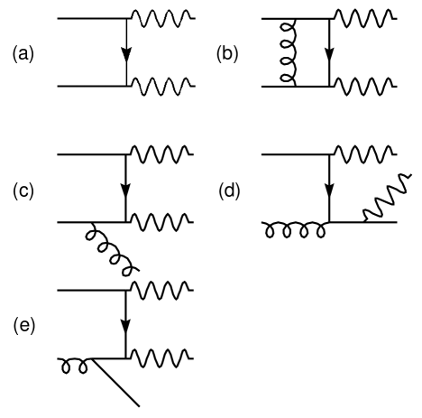
Figure 5.1: A representative set of Feynman diagrams included in the NLO calculation of $Z^{0}$ pair production.

The largest background to the Higgs boson signal in the $Z^{0}Z^{0}$ channel is the continuum production of $Z^{0}$ boson pairs via the $q{\bar{q}}\to Z^{0}Z^{0}X$ partonic subprocess [138]. The next–to–leading order calculations of this process are given in Refs. [126, 127]. A representative set of Feynman diagrams, included in the NLO calculations, is shown in Fig. 5.1. The application of the CSS resummation formalism for the $q\bar{q}\to Z^{0}Z^{0}X$ subprocess is the same as that for the case of $q\bar{q}\to\gamma\gamma X$ [132]. The $A^{(1)}$, $A^{(2)}$ and $B^{(1)}$ coefficients in the Sudakov exponent are identical to those of the Drell–Yan case. This follows from the observation that to produce a heavy $Z^{0}$ boson pair, the virtual–quark line connecting the two $Z^{0}$ bosons in Fig. 5.1 is far off the mass shell, and the leading logarithms due to soft gluon emission beyond the leading order can only be generated from the diagrams in which soft gluons are connected to the incoming (anti–)quark. This situation was described in more detail for di-photon production [132].

The resummed cross section is given by Eq. (5.1), with $i$ and $j$ representing quark and anti–quark flavors, respectively, and

$${\cal F}_{ij}(g,g_{s},\theta,\phi)=2\delta_{ij}(g_{L}^{2}+g_{R}^{2})^{2}\,\frac{1+\cos^{2}\theta}{1-\cos^{2}\theta}.$$

The left- and right-handed couplings $g_{L,R}$ are defined through the $q{\bar{q}Z}^{0}$ vertex, which is written as $i\gamma_{\mu}\left[g_{L}(1-\gamma_{5})+g_{R}(1+\gamma_{5})\right]$, with

$$g_{L}=g\,\frac{T_{3}-s_{w}^{2}Q_{f}}{2c_{w}}~{}~{}~{}{\rm and}~{}~{}~{}g_{R}=-g\,\frac{s_{w}^{2}Q_{f}}{2c_{w}}.$$ (5.4)

Here $g$ is the weak coupling constant, $T_{3}$ is the third component of the SU(2)_L generator ($T_{3}=1/2$ for the up quark $Q_{u}$, and $-1/2$ for the down quark $Q_{d}$), $s_{w}$ ($c_{w}$) is the sine (cosine) of the weak mixing angle, and $Q_{f}$ is the electric charge of the incoming quark in the units of the positron charge ($Q_{u}=2/3$ and $Q_{d}=-1/3$). The values of these parameters will be given in the next section.

The explicit forms of the $A$ and $B$ coefficients, used in the numerical calculations are:

$$A_{q\bar{q}}^{(1)}(C_{1}) = C_{F},$$

$$A_{q\bar{q}}^{(2)}(C_{1}) = C_{F}\left[\left(\frac{67}{36}-\frac{\pi^{2}}{12}\right)N_{C}-\frac{5}{18}N_{f}-2\beta_{1}\ln\left(\frac{b_{0}}{C_{1}}\right)\right],$$

$$B_{q\bar{q}}^{(1)}(C_{1},C_{2}) = C_{F}\left[-\frac{3}{2}-2\ln\left(\frac{C_{2}b_{0}}{C_{1}}\right)\right],$$ (5.5)

where $N_{f}$ is the number of light quark flavors, $N_{C}=3$ is the number of colors in QCD, $C_{F}=4/3$, and $\beta_{1}=(11N_{C}-2N_{f})/12$.

To obtain the value of the total cross section to NLO, it is necessary to include the Wilson coefficients $C_{ij}^{(0)}$ and $C_{ij}^{(1)}$, which can be derived similarly to those for diphoton production in Chapter 4. The results are:

$$C_{jk}^{(0)}(z,b,\mu,{\frac{C_{1}}{C_{2}}},t,u) = \delta_{jk}\delta({1-z}),$$

$$C_{jG}^{(0)}(z,b,\mu,{\frac{C_{1}}{C_{2}}},t,u) = 0,$$

$$C_{jk}^{(1)}(z,b,\mu,{\frac{C_{1}}{C_{2}}},t,u) = \delta_{jk}C_{F}\left\{\frac{1}{2}(1-z)-\frac{1}{C_{F}}\ln\left(\frac{\mu b}{b_{0}}\right)P_{j\leftarrow k}^{(1)}(z)\right.$$

$$\left.+\delta(1-z)\left[-\ln^{2}\left({\frac{C_{1}}{{b_{0}C_{2}}}}e^{-3/4}\right)+{\frac{{\cal V}(t,u)}{4}}+{\frac{9}{16}}\right]\right\},$$

$$C_{jG}^{(1)}(z,b,\mu,{\frac{C_{1}}{C_{2}}},t,u) = {\frac{1}{2}}z(1-z)-\ln\left(\frac{\mu b}{b_{0}}\right)P_{j\leftarrow G}^{(1)}(z).$$ (5.6)

In the above expressions, the splitting kernels are [42]

$$P_{{j\leftarrow k}}^{(1)}(z) = C_{F}\left({\frac{1+z^{2}}{{1-z}}}\right)_{+}~{}~{}~{}{\rm and}$$

$$P_{{j\leftarrow G}}^{(1)}(z) = {\frac{1}{2}}\left[z^{2}+(1-z)^{2}\right].$$ (5.7)

For $Z^{0}$ boson pair production the function ${\cal V}$ in Eq. (5.5) is given by

$${\cal V}(t,u)={\cal V}_{Z^{0}Z^{0}}(t,u)=-4+{\frac{\pi^{2}}{3}}+{\frac{tu}{t^{2}+u^{2}}}\left(F(t,u)+F(u,t)-2\right).$$

The definition of the function $F(t,u)$ is somewhat lengthy and can be found in Appendix C of Ref. [126] (cf. Eqs. (C1) and (C2)). The function ${\cal V}(t,u)$ depends on the kinematic correlation between the initial and final states through its dependence on $t$ and $u$. In the $m_{Z}\to 0$ limit, $F(t,u)+F(u,t)$ reduces to $F^{virt}(t,u)$ of the diphoton case which is given in Ref. [132].

The non-perturbative function used in this study is [73]

$$\widetilde{W}_{q\overline{q}}^{NP}(b,Q,Q_{0},x_{1},x_{2})={\rm exp}\left[-g_{1}b^{2}-g_{2}b^{2}\ln\left({\frac{Q}{2Q_{0}}}\right)-g_{1}g_{3}b\ln{(100x_{1}x_{2})}\right],$$

with $g_{1}=0.11~{}{\rm GeV}^{2}$, $g_{2}=0.58~{}{\rm GeV}^{2}$, $g_{3}=-1.5~{}{\rm GeV}^{-1}$, and $Q_{0}=1.6~{}{\rm GeV}$. These values were fit for the CTEQ2M parton distribution function, with the canonical choice of the renormalization constants, i.e. $C_{1}=C_{3}=b_{0}$ and $C_{2}=1$, and $b_{max}=0.5~{}{\rm GeV}^{-1}$ was used. In principle, these coefficients should be refit for CTEQ4M distributions [38] used in this study. We have checked that using the updated fit in Ref. [140] does not change largely our conclusion because at the LHC and Tevatron energies the perturbative Sudakov contribution is more important compared to that in the low energy fixed target experiments.

Before concluding this section we note that for the diphoton production, we use the formalism described in Ref. [132] to include the $gg\to\gamma\gamma X$ contribution, in which part of the higher order corrections has been included via resummation. Since a gauge invariant calculation of the $gg\to Z^{0}Z^{0}g$ cross section in the SM involves diagrams with the Higgs particle, we shall defer its discussion to a separate work  [131].

5.3 Numerical Results

We implemented our analytic results in the ResBos Monte Carlo event generator [137]. As an input we use the following electroweak parameters [3]:

$$G_{F}=1.16639\times 10^{-5}~{}{\rm GeV}^{-2},~{}~{}m_{Z}=91.187~{}{\rm GeV},$$ (5.8)

$$m_{W}=80.41~{}{\rm GeV},~{}~{}\alpha(m_{Z})=\frac{1}{128.88}.$$

In the on-shell renormalization scheme we define the effective weak mixing angle

$$\sin^{2}\theta_{w}^{eff}=1-\frac{m_{W}^{2}}{\rho m_{Z}^{2}},$$

with

$$\rho=\frac{m_{W}^{2}}{m_{Z}^{2}}\left(1-\frac{\pi\alpha(m_{Z})}{\sqrt{2}G_{F}m_{W}^{2}}\right)^{-1}.$$

In Eq.(5.4), the coupling of the $Z^{0}$ boson to fermions, $g$, is defined using the improved Born approximation:

$$g^{2}=4\sqrt{2}G_{F}(c_{w}^{eff})^{2}m_{Z}^{2}\rho,$$

with $c_{w}^{eff}=\sqrt{1-\sin^{2}\theta_{w}^{eff}}$, the cosine of the effective weak mixing angle. (In Eq. (5.4) $c_{w}$ is identified with $c_{w}^{eff}$.) We use the NLO expression for the running strong and electroweak couplings $\alpha_{s}(\mu)$ and $\alpha(\mu)$, as well as the NLO parton distribution function CTEQ4M (defined in the modified minimal subtraction, i.e. ${\overline{\rm MS}}$, scheme), unless stated otherwise. Furthermore, in all cases we set the renormalization scale equal to the factorization scale: $\mu_{R}=\mu_{F}=Q$.

Di-boson	Collison	$E_{cm}$	Fixed Order ${\cal O}(\alpha_{s}^{0})$		Resummed
produced	type	(TeV)	CTEQ4L	CTEQ4M	$\oplus$ ${\cal O}(\alpha_{s})$
$Z^{0}Z^{0}$	$pp$	14	9.14	10.3	14.8
$Z^{0}Z^{0}$	$p\bar{p}$	2	0.91	1.01	1.64
$\gamma\gamma$	$pp$	14	22.1	24.5	60.8
$\gamma\gamma$	$p\bar{p}$	2	8.48	9.62	22.8
$\gamma\gamma$	$p\bar{p}$	1.8	6.30	7.15	17.0

Table 5.1: Total cross sections of diphoton and $Z^{0}$ boson pair production at the LHC and the upgraded Tevatron, in units of pb. The kinematic cuts are described in the text. The “$\oplus$” sign refers to the matching prescription discussed in the text.

Table 5.1 summarizes the total rates for the leading order (LO), i.e. ${\cal O}(\alpha_{s}^{0})$, and resummed photon- and $Z^{0}$-pair production cross sections for the LHC and the Tevatron. For the lowest order calculation we show results using LO (CTEQ4L) and NLO (CTEQ4M) parton distributions, because there is a noticeable difference due to the PDF choice. As it was discussed in Ref. [137], the resummed total rate is expected to reproduce the ${\cal O}(\alpha_{s})$ rate, provided that in the resummed calculation the $A^{(1)}$, $B^{(1)}$ and $C^{(1)}$ coefficients and the ${\cal O}(\alpha_{s})$ $Y$ piece are included, and the $Q_{T}$ distribution is described by the resummed result for $Q_{T}\leq Q$ and by the ${\cal O}(\alpha_{s})$ result for $Q_{T}>Q$. In our present calculation we added the $A^{(2)}$ coefficient to include the most important higher order corrections in the Sudakov exponent. Our matching prescription (cf. Ref. [137]) is to switch from the resummed prediction to the fixed-order perturbative calculation as they cross around $Q_{T}\sim Q$. This switch is performed for any given $Q$ and $y$ of the photon or $Z^{0}$ boson pairs. In the end, the total cross section predicted by our resummed calculation is about the same as that predicted by the NLO calculation. The small difference of those two predictions can be interpreted as an estimate of the contribution beyond the NLO.

5.3.1 $Z^{0}$ pair production at the LHC

In the LHC experiments the $H\to Z^{0}Z^{0}$ channel can be identified through the decay products of the $Z^{0}$ bosons. The detailed experimental kinematic cuts for this process are given in Ref. [124]. Since the aim of this work is not to analyze the decay kinematics of the background, rather to present the effects of the initial–state soft–gluon radiation, following Ref. [126] for the LHC energies we restrict the rapidities of each $Z^{0}$ bosons as: $|y^{Z}|<3.0$. We do not apply any other kinematic cuts. The total rates are given in Table 5.1. Our ${\cal O}(\alpha_{s}^{0})$ rates are in agreement with that of Ref. [126] when calculated using the same PDF. We expect the resummed rate to be higher than the ${\cal O}(\alpha_{s})$ rate due to the inclusion of the $A^{(2)}$ term. Indeed, our $K$ factor, defined as the ratio of the resummed to the LO rate using the same PDF in both calculations, is higher than the naive soft gluon $K$-factor ($K_{\rm naive}=1+8\pi\alpha_{s}(Q)/9\sim 1.3$) of Ref. [141], which estimates the NLO corrections to the production rate of $q\bar{q}\to Z^{0}Z^{0}X$ in the DIS (deep-inelastic scattering) scheme. Our $K$-factor approaches the naive one with the increase of the center-of-mass energy, as expected.

$E_{cm}$	Collison	$q\bar{q}\to Z^{0}Z^{0}X$	$qg\to Z^{0}Z^{0}X$
(TeV)	type
14	$pp$	10.9	3.91
2	$p\bar{p}$	1.62	0.02

Table 5.2: Resummed cross sections of the subprocesses for $Z^{0}$ boson pair production at the LHC and the upgraded Tevatron, in units of pb. The kinematic cuts are described in the text.

The rates for the different subprocesses of the $Z^{0}$ boson pair production are given in Table 5.2. At the LHC the $qg\to Z^{0}Z^{0}X$ subprocess contributes about 25% of the $qq+qg\to Z^{0}Z^{0}X$ rate. The $K$-factor is defined as the ratio $\sigma(q\bar{q}+qg\to Z^{0}Z^{0}X)/\sigma(q\bar{q}\to Z^{0}Z^{0})$, which is about 1.4 for using CTEQ4M PDF.

Figure 5.2: Transverse momentum distribution of $Z^{0}$ pairs from $q{\bar{q}}+qg$ partonic initial states at the LHC. The ${\cal O}(\alpha_{s})$ (dotted) and the asymptotic (dash-dotted) pieces are coincide and diverge as $Q_{T}\to 0$. The resummed (solid) curve matches the ${\cal O}(\alpha_{s})$ curve at about $Q_{T}=320$ GeV. The resummed $q{\bar{q}}$ contribution (excluding the $qg$ contribution) is shown as dashed line.

Figure 5.3: Invariant mass and rapidity distributions of $Z^{0}$ boson pairs, and transverse momentum distributions of the individual $Z^{0}$ bosons at the LHC. The resummed contribution of the $q{\bar{q}}+qg\to Z^{0}Z^{0}X$ subprocess is shown by the solid curve, and of the $q\bar{q}\to Z^{0}Z^{0}X$ subprocess by the dashed curve. The leading order distribution of $q\bar{q}\to Z^{0}Z^{0}$ is shown by the dash-dotted curve.

Figs. 5.2–5.3 show our results for proton-proton collisions at the LHC energy, $\sqrt{S}=14$ GeV. Fig. 5.2 shows the transverse momentum distribution of $Z^{0}$ pairs. The NLO (${\cal O}(\alpha_{s})$) prediction for the $q{\bar{q}}+qg\to Z^{0}Z^{0}X$ subprocesses, shown by the dotted curve, is singular as $Q_{T}\to 0$. This singular behavior originates from the contribution of terms which grow at least as fast as $1/Q_{T}^{2}$ or $ln(Q^{2}/Q_{T}^{2})/Q_{T}^{2}$. This, so-called asymptotic part, is shown by the dash-dotted curve, which coincides with the ${\cal O}(\alpha_{s})$ distribution as $Q_{T}\to 0$. After exponentiating these terms, the distribution is well behaved in the low $Q_{T}$ region, as shown by the solid curve. The resummed curve matches the ${\cal O}(\alpha_{s})$ curve at about $Q_{T}=320$ GeV. Following our matching prescription described in the previous section, we find that this matching takes place around $Q_{T}=300$ GeV, depending on the actual values of $Q$ and $y$. Fig. 5.2 also shows that at the LHC there is a substantial contribution from $qg$ scattering, which is evident from the difference between the solid and dashed curves, where the dashed curve is the resummed contribution from the $q\bar{q}\to Z^{0}Z^{0}X$ subprocesses.

Figure 5.4: The integrated cross section for $Z^{0}$ boson pair production at the LHC. The resummed and the ${\cal O}(\alpha_{s})$ distributions are shown in solid and dashed lines, respectively.

In Fig. 5.4 we give the integrated distributions, defined as

$$\frac{d\sigma}{dQ_{T}^{\min}}=\int_{Q_{T}^{\min}}^{Q_{T}^{\max}}dQ_{T}\;\frac{d\sigma}{dQ_{T}},$$ (5.9)

where $Q_{T}^{\max}$ is the largest $Q_{T}$ allowed by the phase space. In the NLO calculation, this distribution grows without bound near $Q_{T}^{\min}=0$, as a result of the singular behavior of the scattering amplitude when $Q_{T}\rightarrow 0$. It is clearly shown by Fig. 5.4 that the $Q_{T}$ distribution of the resummed calculation is different from that of the NLO calculation. The different shapes of the two curves in Fig. 5.4 indicates that the predicted $Z^{0}$ pair production rates, with a minimal value of the transverse momentum $Q_{T}$, are different in the two calculations. This is important at the determination of the background for the detection of a Higgs boson even with moderately large transverse momentum. For $Q_{T}^{min}=50$ GeV, the resummed cross section is about 1.5 times of the NLO cross section.

The invariant mass and the rapidity distributions of the $Z^{0}$ boson pairs, and the transverse momentum distribution of the individual $Z^{0}$ bosons are shown in Fig 5.3. When calculating the production rate as the function of the $Z^{0}$ pair invariant mass, we integrate the $Q_{T}$ distribution for any $Q$, and $y$. When plotting the transverse momentum distributions of the individual $Z^{0}$ bosons, we include both of the $Z^{0}$ bosons per event. In the shape of the invariant mass and rapidity distributions we do not expect large deviations from the NLO results. Indeed, the shape of our invariant mass distribution agrees with that in Ref. [126]. However, the resummed transverse momentum distribution $P_{T}^{Z}$ of the individual $Z^{0}$ bosons is slightly broader than the NLO distribution (not shown in Fig 5.3, cf. Ref. [126]). This is expected because, in contrast with the NLO distribution, the resummed transverse momentum distribution of the $Z^{0}$ boson pair is finite as $Q_{T}\rightarrow 0$ so that the $P_{T}^{Z}$ distribution is less peaked.

5.3.2 $Z^{0}$ Pair Production at the upgraded Tevatron

After the upgrade of the Fermilab Tevatron, there are more than $3\times 10^{3}$ $Z^{0}$ boson pairs to be produced. Since this data sample can be used to test the tri-linear gauge boson couplings [136], we also give our results for the upgraded Tevatron with proton–anti-proton collisions at a center-of-mass energy of $2$ TeV. Our kinematic cuts constrain the rapidity of both of the $Z^{0}$ bosons such that $|y^{Z}|<3$. Both the LO and resummed total rates are listed in Table 5.1. The ratio $\sigma(q\bar{q}+qg\to Z^{0}Z^{0}X)/\sigma(q\bar{q}\to Z^{0}Z^{0})$ is about 1.6, which is larger than the naive soft gluon $K$-factor of 1.3. Table 5.2 shows that $qg\to Z^{0}Z^{0}X$ partonic subprocess contributes only a small amount (about 3%) at this energy, in contrast to 25% at the LHC.

Figure 5.5: Same as Fig. 5.3 except for the upgraded Tevatron.

Figure 5.6: Same as Fig. 5.4 except for the upgraded Tevatron.

Figs. 5.5–5.6 show the resummed predictions for the upgraded Tevatron. The invariant mass and rapidity distributions of $Z^{0}$ boson pairs, and the transverse momentum distribution of the individual $Z^{0}$ bosons are shown in Fig. 5.5. The solid curve shows the resummed contributions from the $q{\bar{q}}+qg\to Z^{0}Z^{0}X$ subprocess. The resummed contribution from the $q{\bar{q}}\to Z^{0}Z^{0}X$ subprocess is shown by the dashed curve. The leading order $q{\bar{q}}\to Z^{0}Z^{0}$ cross section is also shown, by the dash-dotted curve. The invariant mass distribution of the $q{\bar{q}}+qg\to Z^{0}Z^{0}X$ subprocess is in agreement with the NLO result of Ref. [126], when calculated for $\sqrt{S}=1.8$ TeV. From this figure we also find that the contribution from the $qg\to Z^{0}Z^{0}X$ subprocess at the energy of the Tevatron is very small.

Figure 5.7: Same as Fig. 5.2 except for the upgraded Tevatron.

In Fig. 5.7 we compare the NLO and resummed distributions of the transverse momentum of the $Z^{0}$ pair. The figure is qualitatively similar to that at the LHC, as shown in Fig. 5.2. The resummed and the NLO curves merge at about 100 GeV. The resummed contribution from the $q{\bar{q}}\to Z^{0}Z^{0}X$ subprocess is shown by the dashed curve, which clearly dominates the total rate.

In Fig. 5.6 we show the integrated distribution $d\sigma/dQ_{T}^{min}$ for $Z^{0}$ boson pair production at the upgraded Tevatron. The figure is qualitatively the same as that for the LHC (cf. Fig. 5.4). The NLO curve runs well under the resummed one in the $Q_{T}^{\min}<$ 80 GeV region, and the $Q_{T}$ distributions from the NLO and the resummed calculations have different shapes even in the region where $Q_{T}$ is of the order 60 GeV. For $Q_{T}^{min}=30$ GeV, the resummed rate is about 1.5 times of the NLO rate.

5.3.3 Diphoton production at the LHC

$E_{cm}$	Collison	$q\bar{q}\to\gamma\gamma X$	$qg\to\gamma\gamma X$	$gg\to\gamma\gamma$		$gg\to\gamma\gamma g$	Fragmen-
(TeV)	type			$4L$	$4M$		tation
14	$pp$	20.5	16.6	22.3	14.4	23.9	6.76
2	$p\bar{p}$	9.68	4.81	6.02	4.34	8.26	2.15

Table 5.3: Cross sections of the subprocesses for diphoton production at the LHC and the upgraded Tevatron, in units of pb. The resummed $qg\to\gamma\gamma X$ rate includes the fragmentation contribution. The ${\cal O}(\alpha_{s}^{2})$ $gg\to\gamma\gamma$ rates were calculated using both the CTEQ4L and CTEQ4M PDF’s. The kinematic cuts are described in the text.

Photon pairs from the decay process $H\to\gamma\gamma$ can be directly detected at the LHC. When calculating its most important background rates, we impose the kinematic cuts on the final state photons that reflect the optimal detection capabilities of the ATLAS detector [124]:

$p_{T}^{\gamma}>25$ GeV, for the transverse momentum of each photons,

$\left|y^{\gamma}\right|<2.5$, for the rapidity of each photons, and

$p_{T}^{1}/(p_{T}^{1}+p_{T}^{2})<0.7$, to suppress the fragmentation contribution, where $p_{T}^{1}$ is the transverse momentum of the photon with the higher $p_{T}$ value.
We also apply a $\Delta R=0.4$ separation cut on the photons, but our results are not sensitive to this cut. (This conclusion is similar to that in Ref. [132].) The total rates and cross sections from the different partonic subprocesses are presented in Tables 5.1 and  5.3. We have incorporated part of the higher order contributions to this process by including $A^{(2)}$ in the Sudakov factor and $C^{(1)}_{gg}$ in the Wilson coefficient functions (cf. Ref. [132]). Within this ansatz, up to ${\cal O}(\alpha_{s}^{3})$, the $gg\to\gamma\gamma X$ rate is about 24 pb, which increases the total $K$-factor by almost 1.0. The leading order $gg\to\gamma\gamma$ rate, via the box diagram, is about 22 pb and 14 pb for using the LO PDF CTEQ4L and the NLO PDF CTEQ4M, respectively. The large difference mainly due to the differences in the strong coupling constants used in the two calculations: CTEQ4L requires $\alpha_{s}(m_{Z})=0.132$, while for CTEQ4M $\alpha_{s}(m_{Z})=0.116$. The ratio $\sigma(q\bar{q}+qg\to\gamma\gamma X)/\sigma(q\bar{q}\to\gamma\gamma)$ is 1.5, and $\sigma(gg\to\gamma\gamma X)/\sigma(q\bar{q}\to\gamma\gamma)$ is about 1. Hence, the ratio of the resummed and the ${\cal O}(\alpha_{s}^{0})$ rates, is quite substantial.

Figure 5.8: Invariant mass and rapidity distributions of photon pairs, and transverse momentum distributions of the individual photons at the LHC. The total resummed contribution (upper solid), and the resummed $q{\bar{q}}+qg\to\gamma\gamma X$ (dashed), $q{\bar{q}}\to\gamma\gamma X$ (dotted), $gg\to\gamma\gamma g$ (dash-dotted), as well as the fragmentation (lower solid) contributions are shown separately. The $q{\bar{q}}\to\gamma\gamma$ ${\cal O}(\alpha_{s}^{0})$ distribution is shown in the middle solid curve.

Figure 5.9: The integrated cross section for photon pair production at the LHC. The resummed and the ${\cal O}(\alpha_{s})$ distributions are shown in solid and dashed lines, respectively.

Figs. 5.8–5.9 show our predictions for distributions of diphotons produced at the LHC. In Fig. 5.8 we plot the invariant mass and rapidity distribution of the photon pairs, and the transverse momentum distribution of the individual photons. When plotting the transverse momentum distributions of the individual photons we include both photons per event. The total (upper solid) and the resummed $q{\bar{q}}+qg\to\gamma\gamma X$ (dashed), $q{\bar{q}}\to\gamma\gamma X$ (dotted), $gg\to\gamma\gamma X$ (dash-dotted), and the fragmentation (lower solid), as well as the leading order $q{\bar{q}}\to\gamma\gamma$ (middle solid) contributions are shown separately. The ratio of the resummed and the LO distributions is about 2.5 which is consistent with the result in Table 5.1. The relative values of the contributions from each subprocesses reflect the summary given in Table 5.3.

Figure 5.10: Transverse momentum distribution of photon pairs at the LHC. The total resummed contribution (upper solid), the resummed $q{\bar{q}}+qg\to\gamma\gamma X$ (dashed), $q{\bar{q}}\to\gamma\gamma X$ (dotted), $gg\to\gamma\gamma X$ (dash-dotted), as well as the fragmentation (lower solid) contributions are shown separately.

Fig. 5.10 shows various contributions to the transverse momentum of the photon pair. At low $Q_{T}$ values ($Q_{T}\ll Q$), the $q{\bar{q}}\to\gamma\gamma X$ contribution is larger than the $qg\to\gamma\gamma X$ contribution, while at high $Q_{T}$ values ($Q_{T}>Q$), the $qg\to\gamma\gamma X$ subprocess becomes more important. The $gg$ contribution dominates the total rate in low $Q_{T}$ region, and the kink in the $gg$ curve at about 50 GeV indicates the need for the inclusion of the complete ${\cal O}(\alpha_{s}^{3})$ $gg\to\gamma\gamma g$ contribution. (Recall that our prediction for the $gg$ contribution at ${\cal O}(\alpha_{s}^{3})$ only holds for small $Q_{T}$, where the effect of the initial-state soft-gluon radiation is relatively more important for a fixed $Q$.)

In Fig. 5.9 we give the integrated cross section as the function of the transverse momentum of the photon pair produced at the LHC. Similarly to the $Z^{0}$ pair production, there is a significant shape difference between the resummed and the NLO curves in the low to mid $Q_{T}$ region. For $Q_{T}^{min}=50$ GeV, the resummed rate is about 1.5 times of the NLO rate.

5.3.4 Diphoton production at the upgraded Tevatron

In Ref. [132], we have presented the predictions of the CSS resummation formalism for the diphoton production at the Tevatron with $\sqrt{S}=1.8$ TeV, and compared with the data [134, 135]. In this Section, we show the results for the upgraded Tevatron with $\sqrt{S}=2.0$ TeV. We use the same kinematic cuts which were used in Ref. [132]:

$p_{T}^{\gamma}>12$ GeV, for the transverse momentum of each photons,

$\left|y^{\gamma}\right|<0.9$, for the rapidity of each photons.
An isolation cut of $\Delta R=0.7$ is also applied. The total cross sections and the rates of the different subprocesses are given by Tables 5.1 and  5.3. The ratio of the $q\bar{q}+qg\to\gamma\gamma X$ and $q\bar{q}\to\gamma\gamma$ rates is about 1.5, similar to that at the LHC. The leading order rate for the $gg\to\gamma\gamma$ subprocess is about 6.0 pb and 4.3 pb for using CTEQ4L and CTEQ4M PDF, respectively. The NLO rate for $gg\to\gamma\gamma g$ is estimated to be 8.3 pb, using the approximation described in Ref. [132], which is about the same magnitude as the leading order $q\bar{q}\to\gamma\gamma$ rate. From our estimate of the NLO $gg$ rate, we expect that the complete ${\cal O}(\alpha_{s}^{3})$ contribution will be important for photon pair production at the Tevatron.

Figure 5.11: Same as Fig. 5.8 but for the upgraded Tevatron.

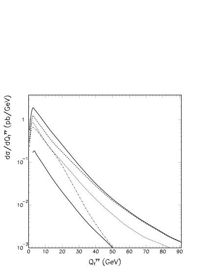
Figure 5.12: Same as Fig. 5.10 but for the upgraded Tevatron.

Figure 5.13: Same as Fig. 5.9 but for the upgraded Tevatron.

Figs. 5.11–5.13 show our results for photon pairs produced at the upgraded Tevatron. The resummed predictions for the invariant mass and rapidity distributions of the photon pairs, and the transverse momentum distribution of the individual photons are shown in Fig. 5.11. In Fig. 5.12 we also plot the contributions to the transverse momentum of the photon pair from the $q{\bar{q}}+qg\to\gamma\gamma X$ (dashed), $q{\bar{q}}\to\gamma\gamma X$ (dotted), $gg\to\gamma\gamma g$ (dash-dotted), and the fragmentation (lower solid) subprocesses, separately. The leading order $q{\bar{q}}\to\gamma\gamma$ cross section (middle solid) is also plotted. In the low $Q_{T}$ region, the $gg$ and the $q\bar{q}$ rates are about the same, and the $qg$ rate becomes more important in the large $Q_{T}$ region. Furthermore, after imposing the above kinematic cuts, the fragmentation contribution is found to be unimportant.

Fig. 5.13 shows the integrated $Q_{T}$ distribution. The qualitative features of these distributions are the same as those predicted for the LHC. For $Q_{T}^{min}=10$ GeV, the resummed cross section is about twice of the NLO cross section.

5.4 Conclusions

In this Section we studied the effects of the initial–state multiple soft–gluon emission on the total rates and various distributions of the most important background processes ($pp,p{\bar{p}}\to\gamma\gamma X,Z^{0}Z^{0}X$) to the detection of the Higgs boson at the LHC. We applied the extended CSS formalism to resum the large logarithms induced by the soft–gluon radiation. We found that for the $q{\bar{q}}$ and $qg$ initiated processes, the total cross sections and the invariant mass distributions of the photon and $Z^{0}$ boson pairs are in agreement with the fixed order calculations. From our estimate of the NLO rate of the $gg$ initiated process, we expect that the complete ${\cal O}(\alpha_{s}^{3})$ contribution will be important for photon pair production at the Tevatron. We showed that the resummed and the NLO transverse momentum distributions of the $Z^{0}$ and photon pairs are substantially different for $Q_{T}{\ \lower-1.2pt\vbox{\hbox{\hbox to0.0pt{$<$\hss}\lower 5.0pt\vbox{\hbox{$\sim$}}}}\ }Q/2$. In terms of the integrated cross section above a given $Q_{T}^{\rm min}$, this difference can be as large as 50% in the low to mid-range of $Q_{T}^{\rm min}$. Using the resummation calculation, we are able to give a reliable prediction of the $Q_{T}$ and any other distribution in the full kinematical region at the LHC and the Tevatron, even in the presence of kinematic cuts. Since the bulk of the signal is in the low transverse momentum region, we conclude that the difference between the NLO and resummed predictions of the background rates will be essential when extracting the signal of the Higgs boson at hadron colliders.

Chapter 6 Charged Scalar Production at Hadron Colliders

6.1 Introduction

The top quark ($t$), among the three generations of fermions, is the only one with a large mass as high as the electroweak scale. This makes the top the most likely place to discover new physics beyond the Standard Model (SM). In a recent study [142], it was proposed that, due to the top-mass enhanced flavor mixing Yukawa coupling of the charm ($c$) and bottom ($b$) with a charged scalar or pseudo-scalar ($\phi^{\pm}$), the $s$-channel partonic process $c\bar{b},\bar{c}b\to\phi^{\pm}$, can be an important mechanism for the production of $\phi^{\pm}$ at various colliders. From the leading order (LO) calculation [142], it was demonstrated that the Fermilab Tevatron Run-II has the potential to explore the mass range of the charged top-pions up to about 300–350 GeV in the topcolor (TopC) models [143, 144]. In this Chapter, we compute the complete next-to-leading order (NLO) QCD corrections to the process $~{}q\bar{q}^{\prime}\to\phi^{\pm}$,  which includes the one-loop virtual corrections and the contributions from the additional ${\cal O}(\alpha_{s})$ processes,

$$q\bar{q}^{\prime}\to\phi^{\pm}g~{}~{}~{}{\rm and}~{}~{}~{}qg\to q^{\prime}\phi^{\pm}.$$ (6.1)

The decay width and branching ratio (BR) of such a (pseudo-)scalar are also included up to NLO to estimate the event rates. The QCD resummation of multiple soft-gluon radiation is also carried out, which provides a better prediction of the transverse momentum distribution of the (pseudo-)scalar particle. We shall choose the TopC model [143] as a benchmark of our analysis. The generalization to the generic type-III two-Higgs doublet model (2HDM) [145, 146] is straightforward since the QCD-corrections are universal. The direct extension to the production of neutral (pseudo-)scalars via $b\bar{b}$ fusion is studied in the Minimal Supersymmetric SM (MSSM) [147, 11] with large $\tan\beta$ and in the TopC models with $U(1)$-tilted large bottom Yukawa coupling [143, 144].

6.2 Charged (Pseudo-)Scalar Production via
Charm-Bottom Fusion

6.2.1 Fixed-Order Calculation

We study charged (pseudo-)scalar production via the top-mass-enhanced flavor mixing vertex $c$-$b$-$\phi^{\pm}$ [142]. The corresponding Yukawa coupling can be generally defined as $~{}{\cal C}_{L}\widehat{L}+{\cal C}_{R}\widehat{R}~{}$ in which $~{}\widehat{L}=(1-\gamma_{5})/2~{}$ and $~{}\widehat{R}=(1+\gamma_{5})/2$ . The total cross sections for the $\phi^{+}$ production at hadron colliders (cf. Fig 1) can be generally expressed as

$$\sigma\left(h_{1}h_{2}\to\phi^{+}X\right)=$$

$$\displaystyle\sum_{\alpha,\beta}\displaystyle\int^{1}_{\tau_{0}}dx_{1}\int^{1}_{\frac{\tau_{0}}{x_{1}}}dx_{2}\left[f_{\alpha/h_{1}}(x_{1},Q^{2})f_{\beta/h_{2}}(x_{2},Q^{2})+(\alpha\leftrightarrow\beta)\right]\widehat{\sigma}^{\alpha\beta}(\alpha\beta\to\phi^{+}X),$$

(6.2)

where $\tau_{0}=m_{\phi}^{2}/S,~{}x_{1,2}=\sqrt{\tau_{0}}\hskip 2.84526pt\displaystyle e^{\pm y}$,  $m_{\phi}$ is the mass of $\phi^{\pm}$, $\sqrt{S}$ is the center-of-mass energy of the $h_{1}h_{2}$ collider, and $f_{\alpha/h}(x,Q^{2})$ is the parton distribution function (PDF) of a parton $\alpha$ with the factorization scale $Q$. The quantity $\widehat{\sigma}^{\alpha\beta}$ is the partonic cross section and has the following LO contribution for $c\bar{b}\to\phi^{+}$ (cf. Fig. 1a) [142]:

$$\widehat{\sigma}^{\alpha\beta}_{\rm LO}~{}=~{}\displaystyle\delta_{\alpha c}\delta_{\beta\bar{b}}\delta(1-\widehat{\tau})\widehat{\sigma}_{0}~{},~{}~{}~{}~{}~{}\widehat{\sigma}_{0}\equiv\frac{\pi}{12\widehat{s}}\left(|{\cal C}_{L}|^{2}+|{\cal C}_{R}|^{2}\right),$$ (6.3)

where  $\widehat{\tau}=m_{\phi}^{2}/\widehat{s}$  with $\widehat{s}$ the center-of-mass energy of the sub-process, and the terms suppressed by the small mass ratio $(m_{c,b}/m_{\phi})^{2}$ have been ignored. Since we are interested in the inclusive production of the scalar $\phi$, it is natural to choose the factorization scale $Q$ to be its mass $m_{\phi}$, which is of ${\cal O}(10^{2-3})$ GeV and much larger than the mass of charm or bottom quark. Hence, in this work, we will treat $c$ and $b$ as massless partons inside proton or anti-proton and perform a NLO QCD calculation with consistent sets of PDFs [148, 149, 150].

The NLO contributions are of ${\cal O}(\alpha_{s})$, which contain three parts: (i) the one-loop Yukawa vertex and quark self-energy corrections (cf. Fig. 1b-d); (ii) the real gluon emission in the $q\bar{q}^{\prime}$-annihilations (cf. Fig. 1e); (iii) $s$- and $t$-channel gluon-quark fusions (cf. Fig. 1f-g). The Feynman diagrams coming from permutations are not shown in Fig. 1. Unlike the usual Drell-Yan type of processes (where the sum of the one-loop quark-wavefunction renormalization and vertex correction gives the ultraviolet finite result), we need to include the renormalization for the Yukawa coupling ($y_{j}$) which usually relates to the relevant quark mass ($m_{q_{j}}$), i.e., we have to add the counter term at the NLO (cf. Fig.1d) besides the contribution from the usual wavefunction renormalization $~{}Z_{q_{1}q_{2}\phi}=\frac{1}{2}(Z_{q_{1}}+Z_{q_{2}})$ (cf. Fig.1c). This applies to the Yukawa interactions of the SM and MSSM Higgs bosons as well as the top-pions in the TopC models. It is clear that, for flavor-mixing vertex $c$-$b$-$\phi^{\pm}$ in the TopC model [cf. Eq. (6.10) below], the counter-term of the Yukawa coupling is equal to the top quark mass counter-term $\delta m_{t}/m_{t}$, which we determine from the top-quark mass renormalization in the on-shell scheme so that $m_{t}$ is the pole mass of the top quark. In other cases such as in the general 2HDM (type-III) [146] and the TopC models (with $b$-Higgs or $b$-pions) [151], some of their Yukawa couplings are not related to quark masses or not of the above simple one-to-one correspondence, and thus have their independent counter terms ($\delta y_{j}/y_{j}$). In addition to the virtual QCD-loop corrections, the contributions of the real gluon emission from the initial state quarks have to be included (cf. Fig. 1e). The soft and collinear singularities appeared in these diagrams are regularized by the dimensional regularization prescription at $D=4-2\epsilon$ dimensions. After summing up the contributions of virtual gluon-loop and real gluon-radiation (cf. Fig. 1b-e), the ultraviolet and soft singularities separately cancel. The collinear singularities are still left over and should be absorbed into the renormalization of the PDF [58]. (The $\overline{\rm MS}$ renormalization scheme is used in our calculation.) Finally, the gluon-quark fusion sub-processes (cf. Fig. 1f-g) should also be taken into account and computed at general dimension-$D$. All these results are separately summarized in Section 6.6.

Figure 6.1: Representative diagrams for charged or neutral (pseudo-)scalar (dashed line) production from quark-antiquark and quark-gluon collisons at ${\cal O}(\alpha_{s}^{0})$ and ${\cal O}(\alpha_{s}^{1})$: (a) leading order contribution; (b-d) self-energy and vertex corrections (with counter term); (e) real gluon radiation in $q\bar{q}^{\prime}$-fusion; (f-g) $s$- and $t$-channel gluon-quark fusions.

The hadron cross sections become regular after renormalizing the Yukawa coupling and the PDFs in (6.2), which are functions of the renormalization scale $\mu$ and the factorization scale $\mu_{F}(=\sqrt{Q^{2}})$. The partonic NLO cross section $\widehat{\sigma}^{\alpha\beta}_{\rm NLO}\left(\alpha\beta\to\phi^{+}X\right)$ contains the contributions $\Delta\widehat{\sigma}_{q\bar{q}^{\prime}}(q\bar{q}^{\prime}\to\phi^{+},\,\phi^{+}g)$, $\Delta\widehat{\sigma}_{qg}(qg\to\phi^{+}q^{\prime})$, and $\Delta\widehat{\sigma}_{\bar{q}g}(\bar{q}g\to\phi^{+}\bar{q}^{\prime})$:

$$\begin{array}[]{l}\left(\Delta\widehat{\sigma}_{q\bar{q}^{\prime}},~{}\Delta\widehat{\sigma}_{qg},~{}\Delta\widehat{\sigma}_{\bar{q}g}\right)=\displaystyle\widehat{\sigma}_{0}\times\frac{\alpha_{s}}{2\pi}\left(\delta_{qc}\delta_{\bar{q}^{\prime}\bar{b}}\Delta\overline{\sigma}_{c\bar{b}},~{}\delta_{qc}\Delta\overline{\sigma}_{cg},~{}\delta_{\bar{q}\bar{b}}\Delta\overline{\sigma}_{\bar{b}g}\right),\\[11.38109pt] \Delta\overline{\sigma}_{c\bar{b}}=\displaystyle C_{F}\left[4\left(1+\widehat{\tau}^{2}\right)\left(\frac{\ln(1-\widehat{\tau})}{1-\widehat{\tau}}\right)_{+}-2\frac{1+\widehat{\tau}^{2}}{1-\widehat{\tau}}\ln\widehat{\tau}\right.\\[11.38109pt] \left.\displaystyle~{}~{}~{}~{}~{}~{}~{}~{}~{}~{}~{}~{}~{}~{}~{}+\left(\frac{2\pi^{2}}{3}-2-\Omega\right)\delta(1-\widehat{\tau})+2(1-\widehat{\tau})\right]+\displaystyle 2P^{(1)}_{q\leftarrow q}(\widehat{\tau})\ln\frac{m_{\phi}^{2}}{Q^{2}}~{},\\[11.38109pt] \Delta\overline{\sigma}_{cg,\bar{b}g}=\displaystyle P^{(1)}_{q\leftarrow g}(\widehat{\tau})\left[\ln\frac{\left(1-\widehat{\tau}\right)^{2}}{\widehat{\tau}}+\ln\frac{m_{\phi}^{2}}{Q^{2}}\right]-\frac{1}{4}(1-\widehat{\tau})\left(3-7\widehat{\tau}\right),\\[17.07164pt] \displaystyle P^{(1)}_{q\leftarrow q}(\widehat{\tau})=\displaystyle C_{F}\left(\frac{1+\widehat{\tau}^{2}}{1-\widehat{\tau}}\right)_{+},~{}~{}~{}~{}\displaystyle P^{(1)}_{q\leftarrow g}(\widehat{\tau})=\frac{1}{2}\left[\widehat{\tau}^{2}+(1-\widehat{\tau})^{2}\right],\end{array}$$ (6.4)

where $~{}\widehat{\tau}=m_{\phi}^{2}/\widehat{s}$ and $C_{F}=4/3$. The mass counter term for the Yukawa vertex renormalization is determined in the on-shell scheme, i.e.,

$$\frac{\delta m_{t}}{m_{t}}=-\frac{C_{F}\alpha_{s}}{4\pi}\left[3\left(\frac{1}{\epsilon}-\gamma_{E}+\ln 4\pi\right)+\Omega\right],$$ (6.5)

in the TopC model. Here, the bare mass $m_{t0}$ and the renormalized mass $m_{t}$ are related by $\,m_{t0}=m_{t}+\delta m_{t}$  and $m_{t}\simeq 175$ GeV is taken to be the top-quark pole mass. The finite part of the mass counter term is $~{}\displaystyle\Omega=3\ln\left[\mu^{2}/m_{t}^{2}\right]+4~{}$ in the TopC model, where $\Omega\geq 0$ for $\mu\geq m_{t}e^{-2/3}\simeq 90$ GeV. In the following, we shall choose the QCD factorization scale $\mu_{F}$ (set as the invariant mass ${\sqrt{Q^{2}}}$) and the renormalization scale $\mu$ to be the same as the scalar mass, i.e., ${\sqrt{Q^{2}}}=\mu=m_{\phi}$, which means that in (6.4) the factor $\ln\left(m_{\phi}^{2}/Q^{2}\right)$ vanishes and the quantity $\Omega$ becomes

$$\Omega=3\ln\left[m_{\phi}^{2}/m_{t}^{2}\right]+4~{}.$$ (6.6)

For the case of $m_{\phi}\gg m_{t}$, the logarithmic term $\ln\left(m_{\phi}^{2}/m_{t}^{2}\right)$ becomes larger for $m_{\phi}\gg m_{t}$, and its contributions to all orders in $\alpha_{s}\ln\left(m_{\phi}^{2}/m_{t}^{2}\right)$ may be resummed by introducing the running Yukawa coupling $y_{t}(\mu)$, or correspondingly, the running mass $m_{t}(\mu)$. In the above formula, $m_{t}$ is the pole mass ($m_{t}^{\rm pol}\simeq 175$ GeV) and is related to the one-loop running mass via the relation [152]

$$m_{t}(\mu)=m_{t}(m_{t}^{\rm pol})\left[1-\frac{3C_{F}}{4\pi}\alpha_{s}(\mu)\ln\frac{\mu^{2}}{m_{t}^{\rm pol}}\right],~{}~{}~{}~{}~{}m_{t}(m_{t}^{\rm pol})=m_{t}^{\rm pol}\left[1+\frac{C_{F}}{\pi}\alpha_{s}(m_{t}^{\rm pol})\right]^{-1}.$$ (6.7)

Using the renormalization group equation, one can resum the leading logarithms to all orders in $\alpha_{s}$ [153] and obtains

$$m_{t}(\mu)=m_{t}(m_{t}^{\rm pol})\left[\frac{\alpha_{s}(\mu)}{\alpha_{s}(m_{t}^{\rm pol})}\right]^{\frac{9C_{F}}{33-2n_{f}}},$$ (6.8)

with $n_{f}=6$ for $\mu>m_{t}$ . Thus, to include the running effect of the Yukawa coupling, we can replace the $(m_{t}^{\rm pol})^{2}$-factor (from the Yukawa coupling) inside the square of the $S$-matrix element [up to ${\cal O}(\alpha_{s})$] by the running factor

$$m_{t}^{2}(\mu)\left\{1+2\frac{C_{F}\alpha_{s}(\mu)}{\pi}\left[1+\frac{3}{4}\ln\left(\frac{\mu}{m_{t}^{\rm pol}}\right)^{2}\right]\right\}\,=\,m_{t}^{2}(\mu)\left[1+\frac{C_{F}\alpha_{s}(\mu)}{2\pi}\Omega\right],$$ (6.9)

where the logarithmic term in the bracket $[\cdots]$ is added to avoid double-counting with the resummed logarithms inside $m_{t}^{2}(\mu)$. It is clear that this $~{}\displaystyle\left[1+\left(C_{F}\alpha_{s}(\mu)/2\pi\right)\Omega\right]~{}$ factor will cancel the $\Omega$-term inside the NLO hard cross section $\Delta\widehat{\sigma}_{c\bar{b}}$ in Eq. (6.4) at ${\cal O}(\alpha_{s})$, so that the net effect of the Yukawa vertex renormalization (after the resummation of leading logarithms) is to replace the relevant tree-level on-shell quark mass (related to the Yukawa coupling) by its $\overline{\rm MS}$ running mass [cf. Eq. (6.8)] and remove the $\Omega$-term in Eq. (6.4). When the physical scale $\mu$ (chosen as the scalar mass $m_{\phi}$) is not much larger than $m_{t}$, the above running effect is small since the $\ln(\mu/m_{t})$ factor in the Yukawa counter-term $\delta m_{t}/m_{t}$ is small. However, the case for the neutral scalar production via the $b\bar{b}$ annihilation can be different. When the loop correction to the $\phi^{0}$-$b$-$\bar{b}$ Yukawa coupling contains the logarithm $\ln(\mu/m_{b})$, which is much larger than $\ln(\mu/m_{t})$, these large logarithms should be resummed into the running coupling, as we will do in Section 4.

In the TopC model, there are three pseudo-scalars, called top-pions, which are predicted to be light, with a mass around of ${\cal O}(100\sim 300)$ GeV. The relevant Yukawa interactions for top-pions, including the large $t_{R}$-$c_{R}$ flavor-mixing, can be written as [142]

$$\begin{array}[]{ll}{\cal L}_{Y}^{\pi_{t}}~{}=&-\displaystyle\frac{m_{t}\tan\beta}{v}\left[iK_{UR}^{tt}{K_{UL}^{tt}}^{\ast}\overline{t_{L}}t_{R}\pi_{t}^{0}+\sqrt{2}{K_{UR}^{tt}}^{\ast}K_{DL}^{bb}\overline{t_{R}}b_{L}\pi_{t}^{+}+\right.\\[8.53581pt] &~{}~{}~{}~{}~{}~{}~{}~{}~{}~{}~{}~{}~{}~{}\left.iK_{UR}^{tc}{K_{UL}^{tt}}^{\ast}\overline{t_{L}}c_{R}\pi_{t}^{0}+\sqrt{2}{K_{UR}^{tc}}^{\ast}K_{DL}^{bb}\overline{c_{R}}b_{L}\pi_{t}^{+}+{\rm h.c.}\right],\end{array}$$ (6.10)

where $\tan\beta=\sqrt{(v/v_{t})^{2}-1}$$\,\sim\!{\cal O}(4\!-\!1.3)$ with the top-pion decay constant $v_{t}\!\sim\!{\cal O}(60\!-\!150$ GeV), and the full vacuum expectation value (vev) $v\simeq 246$ GeV (determined by the Fermi constant). The analysis from top-quark decay in the Tevatron $t\bar{t}$ events sets a direct lower bound on the charged top-pion mass to be larger than about 150 GeV [154, 143]. The existing low energy LEP/SLD measurement of $R_{b}$, which slightly lies above the SM value by about 0.9$\sigma$ [155], also provides an indirect constraint on the top-pion Yukawa coupling ${\cal C}_{R}^{tb}=(\sqrt{2}m_{t}/v)\tan\beta$ due to the one-loop contribution of charged top-pions to $R_{b}$. However, given the crude approximation in estimating the top-pion loops (with all higher loop orders ignored) and the existence of many other sources of contributions associated with the strong dynamics, the indirect $R_{b}$ constraint is not conclusive [143]. For instance, it was shown that the 3$\sigma$ $R_{b}$ bound from the one-loop top-pion correction can be fully removed if the top-pion decay constant $v_{t}$ is increased by a factor of 2 (which can be the typical uncertainty of the Pagels-Stokar estimate) [143, 156]; also, the non-perturbative contributions of coloron-exchanges can shift the $R_{b}$ above its SM value [143] and tend to cancel the negative top-pion corrections. Due to these reasons, it is clear that the inconclusive $R_{b}$-bound in TopC models should not be taken seriously. Nevertheless, to be on the safe side, we will uniformally impose the roughly estimated $R_{b}$-constraint in our current analysis of the TopC model, by including only the (negative) one-loop top-pion contribution as in Ref. [156].

Figure 6.2: Estimated current $3\sigma$-bounds in the TopC model and 2HDM-III: (a) the $3\sigma$ upper bound on the top-pion Yukawa coupling ${\cal C}_{R}^{tb}$; (b) the $3\sigma$ lower bound on the top-pion decay constant; (Here, in (a) and (b), the solid curves are derived from the combined LEP/SLD data of $R_{b}^{\rm Exp}=0.21656\pm 0.00074$ while dashed curves are from the same $3\sigma$ combined experimental error but with the central $R_{b}$-value equal to $R_{b}^{\rm SM}=0.2158$.) (c) the $R_{b}$-predictions of 2HDM-III with coupling $\xi_{tt}=1.0$ and $1.5$ (solid curves) and the $3\sigma$ $R_{b}$-bounds (dashed lines).

As shown in Fig. 6.2a, the current 3$\sigma$ $R_{b}$-bound requires a smaller top-pion Yukawa coupling, ${\cal C}_{R}^{tb}\!\sim\!1.3-2$ (or, $\tan\beta\!\sim\!1.3-2$), for the low mass region of $m_{\pi_{t}^{\pm}}\!\sim\!200-500$ GeV. Since the top-pion decay constant $v_{t}$ is related to $\tan\beta$, this also results in a constraint of $v_{t}$ to be around $150\!\sim\!100$ GeV when $m_{\pi_{t}^{\pm}}\!\sim\!200-500$ GeV (cf. Fig. 6.2b). The usual Pagels-Stokar estimate of $v_{t}$ (by keeping only the leading logarithm but not constant terms) gives $v_{t}\!\sim\!64\!-\!97$ GeV for the topC breaking scale $\Lambda\!\sim\!1\!-\!10$ TeV, where a typical factor of $2\!\sim\!3$ uncertainty in the calculation of $v_{t}^{2}$ is expected  [157, 143]. This estimate is slightly lower than the $R_{b}$-constrained $v_{t}$-values in Fig. 6.2b, but is still in reasonable consistency (given the typical factor of $\sqrt{2}\!\sim\!\sqrt{3}$ error in the leading logarithmic Pagels-Stokar estimate of $v_{t}$).

In (6.10), $K_{UL,R}$ and $K_{DL,R}$ are defined from diagonalizing the up- and down-type quark mass matrices $M_{U}$ and $M_{D}$:  $K_{UL}^{\dagger}M_{U}K_{UR}=M_{U}^{\rm dia},~{}K_{DL}^{\dagger}M_{D}K_{DR}=M_{D}^{\rm dia}~{},$ with $M_{U}^{\rm dia}$$={\rm diag}(m_{u},m_{c},m_{t})$ and $M_{D}^{\rm dia}$$={\rm diag}(m_{d},m_{s},m_{b})$. For the class-I TopC models [151], we have constructed [142] a realistic and attractive pattern of $K_{UL}$ and $K_{DL}$ so that the well-constrained Cabibbo-Kobayashi-Maskawa (CKM) matrix $V~{}(=K_{UL}^{\dagger}K_{DL})$ can be reproduced in the Wolfenstein-parametrization [158] and all potentially large contributions to the low energy data (such as the $K$-$\bar{K}$, $D$-$\bar{D}$ and $B$-$\bar{B}$ mixings and the $b\to s\gamma$ rate) can be avoided [142]. We then found that the right-handed rotation matrix $K_{UR}$ is constrained such that its 33 and 32 elements take the values as [142]

$$K_{UR}^{tt}\simeq 0.99-0.94,~{}~{}~{}K_{UR}^{tc}\leq\sqrt{1-{K_{UR}^{tt}}^{2}}\simeq 0.11-0.33,$$ (6.11)

which show that the $t_{R}$-$c_{R}$ flavor mixing can be naturally around $10-30\%$.

For the current numerical analysis we make the benchmark choice [142] based upon the above TopC model and consider

$${\cal C}^{tb}_{R}={\cal C}_{R}^{tb}(R_{b}{\rm\,constrained}),~{}~{}~{}~{}{\cal C}^{cb}_{R}={\cal C}^{tb}_{R}{K_{UR}^{tc}}\simeq{\cal C}^{tb}_{R}\times 0.2,~{}~{}~{}~{}{\cal C}_{L}^{tb}={\cal C}_{L}^{cb}=0.$$ (6.12)

It is trivial to scale the numerical results presented in this Chapter to any other values of ${\cal C}_{L,R}$ when needed. Unless specified otherwise, we use CTEQ4M PDF [38] to calculate the rates. Note that CTEQ4M PDFs are consistent with the scheme used in the current study which treats the initial state quarks as massless partons in computing the Wilson coefficient functions. The only effect of the heavy quark mass is to determine at which scale $Q$ this heavy quark parton becomes active. In our case, the scale $Q=m_{\phi}\gg m_{c},\,m_{b}$.

In Fig. 6.3, we present the total cross sections for the charged top-pion production as functions of its mass, at the Tevatron (a $p\bar{p}$ collider at 1.8 and 2 TeV) and the LHC (a $pp$ collider at 14 TeV). We compare the improvements by including the complete NLO results [cf. (6.4)] and by including the resummed running Yukawa coupling or running mass [cf. (6.8)]. For this purpose, we first plot the LO total cross sections with the tree-level Yukawa coupling [dash-dotted curves, cf. (6.3) and (6.12)] and with the resummed running Yukawa coupling or running mass [dotted curves, cf. (6.3) and (6.8)]; then we plot the NLO cross sections with the one-loop Yukawa coupling [dashed curves, cf. (6.4)] and with the resummed running Yukawa coupling or running mass [solid curves, cf. (6.4), (6.8) and (6.9)] . We see that at the LHC there is a visible difference between the pure LO results with tree-level Yukawa coupling (dash-dotted curves) and other NLO and/or running-coupling improved results. But at the Tevatron, the LO results with running Yukawa coupling (dotted curves) are visibly smaller than the results in all other cases for $m_{\phi}>300$ GeV. This shows that without the complete NLO calculation, including only the running Yukawa coupling in a LO result may not always warrant a better improvement. Finally, the comparison in Fig. 6.3 shows that the resummed running Yukawa coupling or top-mass [cf. Eq. (6.8)] does not generate any significant improvement from the one-loop running. This is because the top-mass is large and $\alpha_{s}\ln\left(m_{\phi}^{2}/m_{t}^{2}\right)$ is small for $m_{\phi}$ up to 1 TeV. Thus, the improvement of the resummation in (6.8) has to come from higher order effects of $\alpha_{s}\ln\left(m_{\phi}^{2}/m_{t}^{2}\right)$. However, as to be shown in Section 6.5 the situation for summing over powers of $\alpha_{s}\ln\left(m_{\phi}^{2}/m_{b}^{2}\right)$ is different due to $m_{b}\ll m_{t},\,m_{\phi}$ .

Fig. 6.4 is to examine the individual NLO contributions to the charged top-pion production via the $q\bar{q}^{\prime}$ and $qg$ sub-processes, in comparison with the full NLO contributions. The LO contributions are also shown as a reference. [Here $q$ denotes the heavy charm or bottom quark.] In this figure, there are three sets of curves for the charged top-pion production cross sections: the highest set is for the LHC ($\sqrt{S}=14$ TeV), the middle set is for the upgraded Tevatron ($\sqrt{S}=2$ TeV), and the lowest set is for the Tevatron Run I ($\sqrt{S}=1.8$ TeV). The LO cross sections are plotted as dotted lines while the NLO cross sections as solid ones. The dashed lines show the contributions from the $q\bar{q}^{\prime}$-fusion sub-processes, and the dash-dotted lines describe the contributions from the $qg$-fusion sub-processes. The $qg$-fusion cross sections are negative and are plotted by multiplying a factor of $-1$, for convenience. For a quantitative comparison of the individual NLO contributions versus the full NLO results, we further plot, in Fig. 6.5, the ratios (called $K$-factors) of the different NLO contributions to the LO cross section by using the same set of CTEQ4M PDFs. The solid lines of Fig. 6.5 show that the overall NLO corrections to the $pp,p\bar{p}\to\phi^{\pm}X$ processes are positive for $m_{\phi}$ above $\sim$150 (200) GeV and lie below $\sim$15 (10)% for the Tevatron (LHC) in the relevant mass region. This is in contrast with the NLO corrections to the $W^{\pm}$ boson production at hadron colliders, which are always positive and as large as about 25% at the Tevatron [137]. The reason of this difference originates from the differences in the $\Delta\sigma_{q\bar{q}^{\prime}}$ and $\Delta\sigma_{qg,g\bar{q}}$ for $\phi^{\pm}$ and $W^{\pm}$ production. While in the case of $W^{\pm}$ production the positive $\Delta\sigma_{q\bar{q}^{\prime}}$ piece dominates, in the case of $\phi^{\pm}$ production the size of negative $\Delta\sigma_{qg,g\bar{q}}$ piece becomes comparable with that of the positive $\Delta\sigma_{q\bar{q}^{\prime}}$  such that a non-trivial cancellation occurs.

While it is reasonable to take the renormalization and the factorization scales to be $m_{\phi}$ for predicting the inclusive production rate of $\phi^{+}$, it is desirable to estimate the uncertainty in the rates due to different choices of PDFs. For that purpose, we examine a few typical sets of PDFs from CTEQ4, which predict different shapes of charm, bottom and gluon distributions. As shown in Table 6.1 and Fig. 6.6, the uncertainties due to the choice of PDF set are generally within $\pm 20\%$ for the relevant scalar mass ranges at both the Tevatron and the LHC.

Collider	Upgraded Tevatron (2 TeV)				LHC (14 TeV)
Process$\backslash$PDF	4A1	4M	4A5	4HJ	4A1	4M	4A5	4HJ
	367	382	376	387	5380	5800	6060	5890
LO	42.6	43.7	41.5	46.6	863	901	896	906
	6.88	7.05	6.56	8.38	235	240	323	241
	370	402	412	407	5430	6080	6510	6170
NLO	45.6	48.6	47.9	51.6	912	976	997	981
	7.70	8.21	7.89	9.56	255	266	264	268
	551	584	585	590	7530	8290	8740	8400
$q\bar{q}\to\phi^{+}X$	64.5	67.4	65.5	71.7	1210	1280	1290	1290
	10.6	11.1	10.5	13.0	331	341	335	343
	$-$ 180	$-$ 181	$-$ 174	$-$ 183	$-$2100	$-$2200	$-$2240	$-$2230
$qg\to\phi^{+}X$	$-$19.2	$-$18.9	$-$17.5	$-$19.9	$-$299	$-$302	$-$293	$-$303
	$-$2.94	$-$2.86	$-$2.59	$-$3.34	$-$76.0	$-$74.7	$-$70.6	$-$75.0

Table 6.1: Cross sections in fb for charged top-pion production in the TopC model at the upgraded Tevatron and the LHC are shown, by using four different CTEQ4 PDFs. They are separately given for the LO and NLO processes, and for the $q\bar{q}\to\phi^{+}X$ and $qg\to\phi^{+}X$ sub-processes. At the upgraded Tevatron the top number is for $m_{\phi}=200$ GeV, the middle is for $m_{\phi}=300$ GeV, and the lowest is for $m_{\phi}=400$ GeV. At the LHC the top number is for $m_{\phi}=400$ GeV, the middle is for $m_{\phi}=700$ GeV, and the lowest is for $m_{\phi}=1$ TeV.

6.3 Soft-Gluon Resummation

The ${\cal O}(\alpha_{s})$ corrections to the (pseudo-)scalar production involve the contributions from the emission of real and virtual gluons, as shown in Figs. 1(e), (b), and (c). As the result of the real gluon radiation, the (pseudo-)scalar particle will acquire a non-vanishing transverse momentum ($Q_{T}$). When the emitted gluons are soft, they generate large logarithmic contributions of the form: $\alpha_{s}$$\ln^{m}\left(Q^{2}/Q_{T}^{2}\right)$$/Q_{T}^{2}$ (in the lowest order), where $Q$ is the invariant mass of the (pseudo-)scalar, and $m=0,1$. These large logarithms spoil the convergence of the perturbative series, and falsify the ${\cal O}(\alpha_{s})$ prediction of the transverse momentum when $Q_{T}\ll Q$.

To predict the transverse momentum distribution of the produced (pseudo-)scalar, we utilize the Collins–Soper–Sterman (CSS) formalism [44, 45, 46], resumming the logarithms of the type $\alpha_{s}^{n}$ $\ln^{m}\left(Q^{2}/Q_{T}^{2}\right)/Q_{T}^{2}$, to all orders $n$ in $\alpha_{s}$ ($m=0,...,2n-1$). The resummation calculation is performed along the same line as for vector boson production in Chapter 3. Here we only give the differences from that given in Chapter 3. But for convenience, we also list the $A^{(1)}$, $A^{(2)}$, and $B^{(1)}$ coefficients of the Sudakov exponent, which have been used in the current analysis:

$$\begin{array}[]{l}A^{(1)}\left(C_{1}\right)\,=\,C_{F}\,,~{}~{}~{}~{}~{}\,\displaystyle B^{(1)}\left(C_{1}=b_{0},C_{2}=1\right)\,=\,-\frac{3}{2}C_{F}\,,\\[8.53581pt] \displaystyle A^{(2)}\left(C_{1}=b_{0}\right)\,=\,C_{F}\left[\left({\frac{67}{36}}-{\frac{\pi^{2}}{12}}\right)N_{C}-\frac{5}{18}n_{f}\right],\end{array}$$ (6.13)

where $C_{F}=4/3$ is the Casimir of the fundamental representation of SU(3), $N_{C}=3$ is the number of SU(3) colors, and $n_{f}$ is the number of light quark flavors with masses less than $Q$. In the above we used the canonical values of the renormalization constants $C_{1}=b_{0}$, and $\ C_{2}=1$.

To recover the $O\left(\alpha_{s}\right)$ total cross section, we also include the Wilson coefficients $C_{i\alpha}^{(1)}$, among which $C_{ij}^{(1)}$ differs from the vector boson production (here $i$ denotes quark or antiquark flavors, and $\alpha=q_{i}$ or gluon $g$). Explicitly,

$$C_{jk}^{(0)}(z,b,\mu,{{C_{1}}/{C_{2}}}) =~{}\displaystyle\delta_{jk}\delta({1-z}),~{}~{}~{}~{}C_{jg}^{(0)}(z,b,\mu,{C_{1}}/{C_{2}})~{}=~{}0,$$

$$C_{jk}^{(1)}(z,b,\mu,{{C_{1}}/{C_{2}}}) =~{}\displaystyle\delta_{jk}C_{F}\left\{\frac{1}{2}(1-z)-\frac{1}{C_{F}}\ln\left(\frac{\mu b}{b_{0}}\right)P_{j\leftarrow k}^{(1)}(z)\right.$$

$$~{}~{}~{}~{}~{}\displaystyle\left.+\,\delta(1-z)\left[-\ln^{2}\left({\frac{C_{1}}{{b_{0}C_{2}}}}e^{-3/4}\right)+{\frac{\mathcal{V}}{4}}+{\frac{9}{16}}\right]\right\},$$

$$C_{jg}^{(1)}(z,b,\mu,{{C_{1}}/{C_{2}}}) =~{}\displaystyle\frac{1}{2}z(1-z)-\ln\left(\frac{\mu b}{b_{0}}\right)P_{j\leftarrow G}^{(1)}(z),$$ (6.14)

where $P_{j\leftarrow g}^{(1)}$ is the ${\cal O}(\alpha_{s})$ gluon splitting kernels [42] given in Section 1.2.3. In the above expressions, ${\mathcal{V}}={\mathcal{V}}_{DY}=-8+\pi^{2}$ for the vector boson production [137], and ${\mathcal{V}}={\mathcal{V}}_{\Phi}=\pi^{2}$ for the (pseudo-)scalar production, when using the running mass given in Eq. (6.8) for the Yukawa coupling. Using the canonical values of the renormalization constants, $\ln(\mu b/b_{0})$ vanishes, because $\mu=C_{1}/b=b_{0}/b$.

The only remaining difference between the resummed formulae of the vector boson and (pseudo-)scalar production is in the regular ($Y$) terms, which comes from the difference of the $O\left(\alpha_{s}\right)$ real emission amplitude squares (cf., the definitions of ${\cal T}_{q\overline{q}}^{-1}$ and ${\cal T}_{qg}^{-1}$ in Section 2.1.3 and Eqs. (6.22) and (6.25) of this Chapter). The non-perturbative sector of the CSS resummation (the non-perturbative function and the related parameters) is assumed to be the same as that in Ref. [137].

As described in Ref. [137], the resummed total rate is the same as the ${\cal O}(\alpha_{s})$ rate, when we include $C^{(1)}_{i\alpha}$ and $Y^{(1)}$, and switch from the resummed distribution to the fixed order one at $Q_{T}=Q$. When calculating the total rate, we have applied this matching prescription. In the case of the (pseudo-)scalar production, the matching takes place at high $Q_{T}\sim Q$ values, and the above matching prescription is irrelevant when calculating the total rate because the cross sections there are negligible. Thus, as expected, the resummed total rate differs from the ${\cal O}(\alpha_{s})$ rate only by a few percent. Since the difference of the resummed and fixed order rate indicates the size of the higher order corrections, we conclude that for inclusive (pseudo-)scalar production the ${\cal O}(\alpha_{s}^{2})$ corrections are likely much smaller than the uncertainty from the parton distribution functions (cf. Fig.6.5).

In Fig. 6.7, we present the numerical results for the transverse momentum distributions of the charged top-pions (in TopC model) and the charged Higgs bosons (in 2HDM) produced at the upgraded Tevatron and the LHC. The solid curves show the resummation prediction for the typical values of $m_{\phi}$. The dashed curves, from the ${\cal O}(\alpha_{s})$ prediction, are irregular as $Q_{T}\to 0$. The large difference of the transverse momentum distributions between the results from the resummation and fixed-order analyses throughout a wide range of $Q_{T}$ shows the importance of using the resummation prediction when extracting the top-pion and Higgs boson signals. We also note that the average value of $Q_{T}$ varies slowly as $m_{\phi}$ increases and it ranges from 35 to 51 GeV for $m_{\phi}$ between 250 and 550 GeV at the 14 TeV LHC, and from 23 to 45 GeV for $m_{\phi}$ between 200 and 300 GeV at the 2 TeV Tevatron.

Figure 6.3: Top-pion production cross sections at the present Tevatron, upgraded Tevatron, and the LHC. For each collider we show the NLO cross section with the resummed running Yukawa coupling (solid), and with one-loop Yukawa coupling (dashed), as well as the LO cross section with resummed running Yukawa coupling (dotted) and with tree-level (dash-dotted) Yukawa coupling. The cross sections at $\sqrt{S}=1.8$ TeV (thin set of lowest curves) are multiplied by 0.1 to avoid overlap with the $\sqrt{S}=2$ TeV curves.

Figure 6.4: Cross sections for the charged top-pion production in the TopC model at the present Tevatron, upgraded Tevatron and the LHC. The NLO (solid), the $q\bar{q}^{\prime}$ (dashed) and $qg$ (dash-dotted) sub-contributions, and the LO (dotted) contributions are shown. Since the $qg$ cross sections are negative, they are multiplied by $-1$ in the plot. The cross sections at $\sqrt{S}=1.8$ TeV (thin set of lowest curves) are multiplied by 0.1 to avoid overlap with the $\sqrt{S}=2$ TeV curves.

Figure 6.5: The $K$-factors for the $\phi^{+}$ production in the TopC model are shown for the NLO ($K=\sigma_{\rm NLO}/\sigma_{\rm LO}$, solid lines), $q\bar{q}^{\prime}$ ($K=\sigma_{q\bar{q}^{\prime}}/\sigma_{\rm LO}=(\sigma_{\rm LO}+\Delta\sigma_{q\bar{q}^{\prime}})/\sigma_{\rm LO}$, dashed lines), and $qg$ ($K=-\Delta\sigma_{qg}/\sigma_{\rm LO}$, dash-dotted lines) contributions, at the upgraded Tevatron (a) and the LHC (b).

Figure 6.6: The ratios of NLO cross sections computed by four different sets of CTEQ4 PDFs relative to that by the CTEQ4M for charged top-pion production at the upgraded Tevatron (a) and the LHC (b).

Figure 6.7: Transverse momentum distributions of charged top-pions produced in hadronic collisions. The resummed (solid) and ${\cal O}(\alpha_{s})$ (dashed) curves are calculated for $m_{\phi}=$ 200, 250, and 300 GeV at the upgraded Tevatron (a), and for $m_{\phi}=$ 250, 400, and 550 GeV at the LHC (b).

6.4 Hadronic Decays of Charged (Pseudo-)Scalars to ${\cal O}(\alpha_{s})$

In the TopC models, the current Tevatron data from the top quark decay into charged top-pion ($\pi_{t}^{\pm}$) and $b$-quark already requires the mass of $\pi_{t}^{\pm}$ to be above $\sim$150 GeV [143, 154]. In the current analysis, we shall consider $m_{\pi_{t}}>m_{t}+m_{b}$, so that its dominant decay channels are $\pi_{t}^{\pm}\to tb,cb$ .

The decay width of $\pi_{t}^{\pm}$ ($=\phi^{\pm}$), including the ${\cal O}(\alpha_{s})$ QCD corrections, is given by [160, 161]:

$$\begin{array}[]{l}\displaystyle\Gamma_{\rm NLO}(Q)~{}=~{}\displaystyle\Gamma_{\rm LO}(Q)\left[1+\frac{\alpha_{s}C_{F}}{2\pi}{\cal R}\right],{}{}{}{}{}\\[8.53581pt] \Gamma_{\rm LO}(Q)~{}=\displaystyle\frac{3}{16\pi}Q\left(|{\cal C}_{L}|^{2}+|{\cal C}_{R}|^{2}\right)(1-r)^{2},\\[7.96677pt] {\cal R}~{}=~{}\displaystyle\frac{9}{2}(1-r)^{2}+(1-r)\left(3-7r+2r^{2}\right)\ln\frac{r}{1-r}+\left[\displaystyle 3\ln\frac{Q^{2}}{m_{t}^{2}}+4-\Omega\right]\\[6.54413pt] ~{}~{}~{}~{}~{}~{}~{}~{}\displaystyle-2(1-r)^{2}\left[\frac{\ln(1-r)}{1-r}-2{\rm Li}_{2}\left(\frac{r}{1-r}\right)-\ln(1-r)\ln\frac{r}{1-r}\right],\end{array}$$ (6.15)

in which $Q=\sqrt{Q^{2}}$ is the invariant mass of $\phi^{\pm}$. The small bottom and charm masses are ignored so that  $r\equiv\left(m_{t}/m_{\phi}\right)^{2}$ for $tb$ final state and $~{}r=0~{}$ for $cb$ final state. Thus, for $~{}\phi^{\pm}\to cb$,  the quantity ${\cal R}$ reduces to $\,{\cal R}={17}/{2}-\Omega$ . In Fig. 6.8, we present the results for total decay widths of $\phi^{+}$ and branching ratios of $\phi^{+}\to t\bar{b}$ in the TopC model and the 2HDM. For the 2HDM, we also show the branching ratios of the $W^{+}h^{0}$ channel, which is complementary to the $t\bar{b}$ channel. The NLO (solid) and LO (dashed) curves differ only by a small amount. In the same figure, the $K$-factor, defined as the ratio of the NLO to the LO partial decay widths, is plotted for the $\phi^{+}\to t\bar{b}$ (solid) and $\to c\bar{b}$ (dashed) channels. Here, the sample results for the 2HDM are derived for the parameter choice: $\alpha=0$ and $(M_{h},\,M_{A})=(100,\,1200)$ GeV.

With the decay width given above, we can study the invariant mass distribution of $\,tb\,$ for the $s$-channel $\phi^{+}$-production:

$$\frac{d\sigma}{dQ^{2}}\left[h_{1}h_{2}\to(\phi^{+}X)\to t\bar{b}X\right]=\displaystyle\sigma\left[h_{1}h_{2}\to\phi^{+}(Q)X\right]\frac{\left(Q^{2}\Gamma_{\phi}/m_{\phi}\right){\rm Br}\left[\phi^{+}\to t\bar{b}\right]}{\pi\left[\left(Q^{2}-m_{\phi}^{2}\right)^{2}+\left(Q^{2}\Gamma_{\phi}/m_{\phi}\right)^{2}\right]},$$ (6.16)

where $\Gamma_{\phi}$ and ${\rm Br}\left[\phi^{+}\to t\bar{b}\right]$ are the total decay width of $\phi^{+}$ and the branching ratio of $\phi^{+}\to t\bar{b}$, respectively, which are calculated up to the NLO. We note that the one-loop box diagrams with a virtual gluon connecting the initial state quark and final state quark (from the hadronic decay of $\phi$) have vanishing contribution at ${\cal O}(\alpha_{s})$ because the scalar $\phi$ is color-neutral. In Fig. 6.9a and Fig. 6.10a, we plot the invariant mass distribution for $t$-$\bar{b}$ and $\bar{t}$-$b$ pairs from $\phi^{\pm}$ (top-pion signal) and $W^{\pm\ast}$ (background) decays in the TopC model. In these plots, we have included the NLO contributions, as a function of $Q$, to the $W^{\pm\ast}$ background rate at the Tevatron and the LHC. The overall $K$-factor (after averaging over the invariant mass $Q$) including both the initial and final state radiations is about 1.4 (1.34) for the Tevatron (LHC) [162]. The total rate of $W^{\pm\ast}$ up to the NLO is about 0.70 [0.86] pb and 11.0 pb at the 1.8 [2] TeV Tevatron and the 14 TeV LHC, respectively.

Figure 6.8: Total decay widths of $\phi^{+}$ and BRs of $\phi^{+}\to t\bar{b}$ in the TopC model and 2HDM. (For the 2HDM, the BR of the $W^{+}h^{0}$ channel is also shown, which is complementary to the $t\bar{b}$ channel.) In Fig. (a) and (b), the NLO (solid) and LO (dashed) curves differ only by a small amount. In Fig. (c), the $K$-factor, which is defined as the ratio of the NLO to the LO partial decay widths, is shown for the $\phi^{+}\to t\bar{b}$ (solid) and $\to c\bar{b}$ (dashed) channels. The sample results for the 2HDM in this figure are derived for the parameter choice $(\xi_{tt}^{U},\,\xi_{tc}^{U})=(1.5,\,1.5)$, $\alpha=0$, and $(m_{h},\,m_{A})=(120,\,1200)$ GeV.

Figure 6.9: Invariant mass distribution of $t$-$\bar{b}$ and $\bar{t}$-$b$ pairs from $\phi^{\pm}$ (signal) and $W^{\pm*}$ (background) decays at the Tevatron Run-II for the TopC model (a), and 2HDM with Higgs mixing angles $\alpha=0$ (b), and $\alpha=\pi/2$ (c). We show the signal for $m_{\phi}=200,~{}250$, 300 and 350 GeV. The solid curves show the results from the NLO calculation, and the dashed ones from the LO analysis.

Figure 6.10: Invariant mass distribution of $t$-$\bar{b}$ and $\bar{t}$-$b$ pairs from $\phi^{\pm}$ (signal) and $W^{\pm*}$ (background) decays at the LHC for the TopC model (a), and for the 2HDM with the Higgs mixing angles $\alpha=0$ in (b), and $\alpha=\pi/2$ in (c). Here the charged pseudo-scalar or scalar mass are chosen as the typical values of $m_{\phi}=250,~{}400$ and 550 GeV. The solid curves show the results by the NLO calculation, while the dashed ones come from the LO analysis.

Figure 6.11: Invariant mass distributions of $W^{+}$-$h^{0}$ and $W^{-}$-$h^{0}$ pairs from $\phi^{\pm}$ ($s$-channel resonance) and $W^{\pm*}$ ($s$-channel non-resonance) decays at the Tevatron Run-II, and at the LHC, for the 2HDM with Higgs mixing angles $\alpha=0$. We show the signal for $m_{\phi}=200,~{}250$ and 300 GeV at the Tevatron (a), and for $m_{\phi}=250,~{}400$ and 550 GeV at the LHC (b). The solid curves show the results of the NLO calculation, and the dashed ones of the LO analysis.

Before concluding this section, we discuss how to generalize the above results to the generic 2HDM (called type-III [146]), in which the two Higgs doublets $\Phi_{1}$ and $\Phi_{2}$ couple to both up- and down-type quarks and the ad hoc discrete symmetry [163] is not imposed. The flavor-mixing Yukawa couplings in this model can be conveniently formulated under a proper basis of Higgs doublets so that $~{}<\Phi_{1}>=(0,v/\sqrt{2})^{T}$ and $<\Phi_{2}>=(0,0)^{T}$. Thus, the diagonalization of the fermion mass matrix also diagonalizes the Yukawa couplings of $\Phi_{1}$, and all the flavor-mixing effects are generated by Yukawa couplings ($\widehat{Y}^{U}_{ij}$ and $\widehat{Y}^{D}_{ij}$) of $\Phi_{2}$ which exhibit a natural hierarchy under the ansatz [145, 146]

$$\widehat{Y}_{ij}^{U,D}=\xi_{ij}^{U,D}{\sqrt{m_{i}m_{j}}}/{<\Phi_{1}>}$$ (6.17)

with $~{}\xi_{ij}^{U,D}\sim{\cal O}(1)$.  This ansatz highly suppresses the flavor-mixings among light quarks and identifies the largest mixing coupling as the one from the $t$-$c$ or $c$-$t$ transition. A recent renormalization group analysis [164] shows that such a suppression persists at the high energy scales. The relevant Yukawa interactions involving the charged Higgs bosons $H^{\pm}$ are [142]:

$$\begin{array}[]{ll}&{\cal L}_{Y}^{CC}=\\[5.69054pt] &~{}H^{+}\left[\overline{t_{R}}~{}(\widehat{Y}_{U}^{\dagger}V)_{tb}~{}b_{L}-\overline{t_{L}}~{}(V\widehat{Y}_{D})_{tb}~{}b_{R}~{}+\overline{c_{R}}~{}(\widehat{Y}_{U}^{\dagger}V)_{cb}~{}b_{L}-\overline{c_{L}}~{}(V\widehat{Y}_{D})_{cb}~{}b_{R}~{}\right]+{\rm h.c.}\\[5.69054pt] &~{}\simeq~{}H^{+}\left[\overline{t_{R}}~{}\widehat{Y}^{U\ast}_{tt}~{}b_{L}+\overline{c_{R}}~{}\widehat{Y}^{U\ast}_{tc}~{}b_{L}\right]+{\rm h.c.}+({\rm small~{}terms})\,,\end{array}$$ (6.18)

where $~{}\widehat{Y}^{U}_{tt}=\xi^{U}_{tt}\times(\sqrt{2}m_{t}/v)\simeq\xi^{U}_{tt}$, and $~{}\widehat{Y}^{U}_{tc}=\xi^{U}_{tc}\times(\sqrt{2m_{t}m_{c}}/v)\simeq\xi^{U}_{tc}\times 9\%~{}$, in which $~{}\xi^{U}_{tc}\sim{\cal O}(1)$ is allowed by the current low energy data [146, 165]. As a result, the Yukawa counter term in Fig. 1d involves both $\delta m_{t}$ and $\delta m_{c}$. Consequently, we need to replace the NLO quantity $\Omega$ in the finite part of the Yukawa counter term [cf. the definition below (6.4)] by

$$\Omega({\rm 2HDM})=3\ln\left[m_{\phi}^{2}/(m_{t}m_{c})\right]+4~{},$$ (6.19)

for the type-III 2HDM. In the relevant $\phi^{\pm}$-$c$-$b$ coupling of this 2HDM, we note that, similar to the case of the TopC model, only the right-handed charm is involved [142], i.e.,

$${\cal C}_{L}^{tb}={\cal C}_{L}^{cb}=0,~{}~{}~{}~{}{\cal C}_{R}^{tb}=\xi_{tt}^{U}(\sqrt{2}m_{t}/v),~{}~{}~{}{\cal C}_{R}^{cb}\simeq\xi^{U}_{tc}\times 9\%.$$ (6.20)

where the parameters ($\xi^{U}_{tt},\,\xi_{tc}^{U}$) are expected to be naturally around ${\cal O}(1)$. We have examined the possible constraint of $\xi^{U}_{tt}$ from the current $R_{b}$ data and found that the typical values of $\xi^{U}_{tt}\!\sim\!1.0\!-\!1.5$ are allowed for $m_{H^{\pm}}{\ \lower-1.2pt\vbox{\hbox{\hbox to0.0pt{$>$\hss}\lower 5.0pt\vbox{\hbox{$\sim$}}}}\ }200$ GeV (cf. Fig. 6.2c).  The production cross section of $H^{\pm}$ in this 2HDM can be obtained by rescaling the result of the TopC model according to the ratio of the coupling-square $\left[{\cal C}^{tc}_{R}({\rm 2HDM})/{\cal C}_{R}^{tc}({\rm TopC})\right]^{2}\!\sim\!\left[0.09\xi_{tc}^{U}/0.2{\cal C}_{R}^{tb}({\rm TopC})\right]^{2}$ (which is about $1/7$ for $\xi_{tc}^{U}=1.5$ and the charged scalar mass around $400$ GeV).

Finally, we note that there are three neutral Higgs bosons in the 2HDM, the CP-even scalars ($h^{0},~{}H^{0}$) and the CP-odd pseudo-scalar $A^{0}$. The mass diagonalization for $h^{0}$ and $H^{0}$ induces the Higgs mixing angle $\alpha$. The low energy constraints on this model require [146, 165] $~{}m_{h},\,m_{H}\leq m_{H^{\pm}}\leq m_{A}~{}$ or $~{}m_{A}\leq m_{H^{\pm}}\leq m_{h},\,m_{H}$.  For the case of $m_{H^{\pm}}>m_{h^{0}}+M_{W}$, the $H^{\pm}\to W^{\pm}h^{0}$ decay channel is also open. Taking, for example, $\alpha=0$ and $(m_{h},\,m_{A})=(120,1200)$ GeV, we find from Fig. 6.8b that the $tb$ and $Wh^{0}$ decay modes are complementary at low and high mass regions of the charged Higgs boson $H^{\pm}$. In Figs. 6.9b-c and 6.10b-c, we plot the invariant mass distributions of $t\bar{b}$ and $\bar{t}b$ pairs from $H^{\pm}$ (signal) and $W^{\pm\ast}$ (background) decays in the 2HDM at the 2 TeV Tevatron and the 14 TeV LHC, with the typical choice of the parameters: $~{}\left(\xi^{U}_{tt},\,\xi^{U}_{tc}\right)=(1.5,\,1.5)$ in Eq. (6.20), $\left(m_{h},\,m_{A}\right)=\left(120,\,1200\right)$ GeV, and $\alpha=0$ or $\pi/2$. [A larger value of $\xi^{U}_{tt}$ will simultaneously increase (reduce) the BR of $tb$ ($Wh^{0}$) mode.] We see that, due to a smaller $c$-$b$-$H^{\pm}$ coupling [cf. (6.20)], it is hard to detect such a charged Higgs boson with mass $m_{H^{\pm}}>250$ GeV at the Tevatron Run-II. We then examine the potential of the LHC for the high mass range of $H^{\pm}$. Similar plots are shown in Figs. 6.9b-c for $\alpha=0$ and $\alpha=\pi/2$, respectively. When $\cos\alpha$ is large (e.g., $\alpha=0$), the branching ratio of the $tb$-channel decreases as $m_{H^{\pm}}$ increases (cf. Fig. 6.8b), so that the LHC does not significantly improve the probe of the large $m_{H^{\pm}}$, range via the single-top mode (cf. Fig. 6.10b). In this case, the $W^{\pm}h^{0}$ channel, however, becomes important for large $m_{H^{\pm}}$, as shown in Fig. 6.11 (cf. Fig. 6.8b, for its decay branching ratios) since the $H^{\pm}$-$W^{\mp}$-$h^{0}$ coupling is proportional to $\cos\alpha$ [146]. On the other hand, for the parameter space with small $\cos\alpha$ (e.g., $\alpha=\pi/2$), the $W^{\pm}h^{0}$ channel is suppressed so that the single-top mode is important even for large mass region of $H^{\pm}$.  This is illustrated in Fig. 6.10c at the LHC for $\alpha=\pi/2$. In order to probe the whole parameter space and larger $m_{H^{\pm}}$, it is important to study both $tb$ and $Wh^{0}$ (or $WH^{0}$) channels.

6.5 Generalization to Neutral (Pseudo-)Scalar
Production via $b\bar{b}$ Fusion

The QCD corrections are universal so that the generalization to the production of neutral scalar or pseudo-scalar $\phi^{0}$ via the $b\bar{b}$ fusion is straightforward, i.e., we only need to replace (6.19) by

$$\Omega(\phi^{0}b\bar{b})=3\ln\left[m_{\phi}^{2}/m_{b}^{2}\right]+4\,,$$ (6.21)

in which $m_{\phi}$ is the mass of $\phi^{0}$. The finite piece of the Yukawa renormalization [cf. the quantity $\Omega$ in (6.5)] is scheme-dependent. We can always define the $\phi^{0}$-$b$-$\bar{b}$ Yukawa coupling as $\sqrt{2}m_{b}/v$ times an enhancement factor $K$ so that the Yukawa counter term is generated by $\delta m_{b}/m_{b}$. After resumming the leading logarithmic terms, $\left[\alpha_{s}\ln(m_{\phi}^{2}/m_{b}^{2})\right]^{n}$, via the renormalization group technique, the net effect of the Yukawa renormalization is to change the Yukawa coupling or the related quark-mass into the corresponding $\overline{\rm MS}$ running coupling or mass, as discussed in the previous section.

The $b\bar{b}$ decay branching ratios of the neutral Higgs bosons in the MSSM with large $\tan\beta$ are almost equal to one [168]. The same is true for the $b$-Higgs or $b$-pion in the TopC model [143]. It has been shown that at the Tevatron, the $b\bar{b}$ di-jet final states can be properly identified [169]. The same technique developed for studying the resonance of the coloron or techni-$\rho$ in the $b\bar{b}$ decay mode [169] can also be applied to the search of the neutral Higgs bosons with large bottom Yukawa coupling. When the neutral scalar or pseudo-scalar $\phi^{0}$ is relatively heavy, e.g., in the range of ${\cal O}(250-1000)$ GeV, the QCD di-jet backgrounds can be effectively removed by requiring the two $b$-jets to be tagged with large transverse momenta ($P_{T}$) because the $P_{T}$ of each $b$-jet from the $\phi^{0}$ decay is typically at the order of $m_{\phi}/2$. Hence, this process can provide complementary information to that obtained from studying the $\phi^{0}b\bar{b}$ associate production [170, 167, 171].

We first consider the production of the neutral Higgs boson $\phi^{0}$, which can be either $A^{0}$, $h^{0}$, or $H^{0}$, in the MSSM with large $\tan\beta$, where the corresponding Yukawa couplings to $b\bar{b}$ and $\tau^{+}\tau^{-}$ are enhanced relative to that of the SM since $y_{D}/y_{D}^{\rm SM}$ is equal to $\tan\beta$, $-\sin\alpha/\cos\beta$, or $\cos\alpha/\cos\beta$, respectively, at the tree-level. In the large $\tan\beta$ region, the MSSM neutral Higgs bosons dominantly decay into $b\bar{b}$ and $\tau^{+}\tau^{-}$ final states, which can be detected at the hadron colliders. In comparison with the recent studies on the $\phi^{0}b\bar{b}$ [167] and $\phi^{0}\tau^{+}\tau^{-}$ [172] associate production, we expect the inclusive $\phi^{0}$ production via the $b\bar{b}$-fusion would be more useful for $m_{\phi}$ being relatively heavy (e.g., $m_{\phi}\geq 200-300$ GeV) because of the much larger phase space as well as a better suppression of the backgrounds in the high $P_{T}$ region. The total LO and NLO cross sections for the inclusive production process $pp,p\bar{p}\to A^{0}X$ at the Tevatron and the LHC are shown in Figs. 6.12a and b, in parallel to Figs. 6.3 and 6.4 for the case of charged top-pion production. Here, we have chosen  $\tan\beta=40$  for illustration. The cross sections at other values of $\tan\beta$ can be obtained by multiplying the scaling factor $\,\left(\tan\beta/40\right)^{2}\,$. From Fig. 6.12a, we see a significant improvement from the pure LO results (dash-dotted curves) by resumming over the large logarithms of $m_{\phi}^{2}/m_{b}^{2}$ into the running Yukawa coupling. The good agreement between the LO results with running Yukawa coupling and the NLO results is due to a non-trivial, and process-dependent, cancellation between the individual ${\cal O}(\alpha_{s})$ contributions of the $b\bar{b}$ and $bg$ sub-processes. In contrast to the production of the charged top-pion or Higgs boson via the initial state $c\bar{b}$ or $\bar{c}b$ partons, the neutral Higgs boson production involves the $b\bar{b}$ parton densities. The $K$-factors for the ratios of the NLO versus LO cross sections of $p\bar{p}/pp\to A^{0}X$ are presented in Fig. 6.13 for the MSSM with $\tan\beta=40$. The main difference is due to the fact that the individual contribution by the ${\cal O}(\alpha_{s})$ $bg$-fusion becomes more negative as compared to the case of the charged top-pion production shown in Fig. 6.5. This makes the overall $K$-factor of the NLO versus LO cross sections range from about $-(16$$\sim$17)% to +5% at the Tevatron and the LHC. In parallel to Table 1 and Fig. 6.6, we have examined the uncertainties of the CTEQ4 PDFs for the $A^{0}$-production at the Tevatron and the LHC, and the results are summarized in Table 6.2 and Fig. 6.14).

The transverse momentum ($Q_{T}$) distributions of $A^{0}$, produced at the upgraded Tevatron and at the LHC, are shown in Fig. 6.15 for various $A^{0}$ masses ($m_{A}$) with $\tan\beta=40$. The solid curves are the result of the multiple soft-gluon resummation, and the dashed ones are from the ${\cal O}(\alpha_{s})$ calculation. The shape of these transverse momentum distributions is similar to that of the charged top-pion (cf. Fig. 6.7). The fixed order distributions are singular as $Q_{T}\to 0$, while the resummed ones have a maximum at some finite $Q_{T}$ and vanish at $Q_{T}=0$. When $Q_{T}$ becomes large, of the order of $m_{A}$, the resummed curves merge into the fixed order ones. The average resummed $Q_{T}$ varies between 25 and 30 (40 and 60) GeV in the mass range of $m_{A}$ from 200 to 300 (250 to 550) GeV at the Tevatron (LHC).

We also note that for large $\tan\beta$, the SUSY correction to the running $\phi^{0}$-$b$-$\bar{b}$ Yukawa coupling is significant [173] and can be included in a way similar to our recent analysis of the $\phi^{0}b\bar{b}$ associate production [167]. To illustrate the SUSY correction to the $b$-Yukawa coupling, we choose all MSSM soft-breaking parameters as $500$ GeV, and the Higgs mixing parameter $\mu=\pm 500$ GeV. Depending on the sign of $\mu$, the SUSY correction to the $\phi^{0}$-$b$-${\bar{b}}$ coupling can either take the same sign as the QCD correction or have an opposite sign [167]. In Fig. 6.12c, the solid curves represent the NLO cross sections with QCD correction alone, while the results including the SUSY corrections to the running bottom Yukawa coupling are shown for $\mu=+500$ GeV (upper dashed curves) and $\mu=-500$ GeV (lower dashed curves). As shown, these partial SUSY corrections can change the cross sections by about a factor of 2. The above results are for the inclusive production of the CP-odd Higgs boson $A^{0}$ in the MSSM. Similar results can be easily obtained for the other neutral Higgs bosons ($h^{0}$ and $H^{0}$) by properly rescaling the coupling strength. We also note that in the large $\tan\beta$ region, there is always a good mass-degeneracy between either $h^{0}$ and $A^{0}$ (in the low mass region with $m_{A}\stackrel{{\scriptstyle<}}{{\sim}}120$ GeV) or $H^{0}$ and $A^{0}$ (in the high mass region with $m_{A}\stackrel{{\scriptstyle>}}{{\sim}}120$ GeV), as shown in Figs. 10 and 11 of Ref. [167].

Collider	Upgraded Tevatron (2 TeV)				LHC (14 TeV)
Process$\backslash$PDF	4A1	4M	4A5	4HJ	4A1	4M	4A5	4HJ
	2020	1900	1660	1920	18100	19800	16600	17900
LO	166	153	129	163	1520	1440	1280	1440
	19.9	18.2	15.0	21.7	258	238	206	238
	1810	1780	1620	1800	17100	17400	16700	17500
NLO	160	154	134	164	1520	1470	1350	1470
	20.3	19.3	16.4	22.9	265	250	222	251
	3040	2900	2590	2930	25400	25400	24100	25600
$q\bar{q}\to\phi^{0}X$	253	237	203	251	2140	2050	1850	2050
	31.0	28.8	24.0	33.8	364	339	298	340
	$-$1230	$-$1120	$-$970	$-$1130	$-$8320	$-$8010	$-$7370	$-$8050
$qg\to\phi^{0}X$	$-$92.9	$-$83.1	$-$69.0	$-$87.5	$-$623	$-$575	$-$505	$-$574
	$-$10.6	$-$9.42	$-$7.59	$-$10.9	$-$98.8	$-$88.8	$-$75.8	$-$88.7

Table 6.2: Cross sections in fb for neutral Higgs boson production in the MSSM with $\tan\beta=40$, at the upgraded Tevatron and the LHC, are shown for four different CTEQ4 PDFs. They are separately given for the LO and NLO processes, and for the $b\bar{b}\to A^{0}X$ and $bg\to A^{0}X$ sub-processes. For the upgraded Tevatron the top number is for $m_{A}=200$ GeV, the middle is for $m_{A}=300$ GeV, and the lowest is for $m_{A}=400$ GeV. For the LHC the top number is for $m_{A}=400$ GeV, the middle is for $m_{A}=700$ GeV, and the lowest is for $m_{A}=1$ TeV.

Figure 6.12: LO and NLO cross sections for the neutral Higgs $A^{0}$ production in the MSSM with $\tan\beta=40$, at the Tevatron and the LHC. (a) For each collider we show the NLO cross sections with the resummed running Yukawa coupling (solid) and with one-loop Yukawa coupling (dashed), as well as the LO cross sections with resummed running Yukawa coupling (dotted) and with tree-level Yukawa coupling (dash-dotted). (b) The NLO (solid), the $b\bar{b}$ (dashed) and $bg$ (dash-dotted) sub-contributions, and the LO (dotted) contributions are shown. Since the $bg$ cross sections are negative, they are multiplied by $-1$ in the plot. The cross sections at $\sqrt{S}=1.8$ TeV (thin set of lowest curves) are multiplied by 0.1 to avoid overlap with the $\sqrt{S}=2$ TeV curves. (c) The NLO cross sections with QCD running Yukawa coupling (solid curves) and those with additional SUSY correction to the running coupling are shown (upper dashed lines for the Higgs-mixing parameter $\mu=+500$ GeV and lower dashed lines for $\mu=-500$ GeV).

Figure 6.13: The $K$-factors for the $A^{0}$ production in the MSSM with $\tan\beta=40$ are shown for the NLO ($K=\sigma_{\rm NLO}/\sigma_{\rm LO}$, solid lines), $b\bar{b}$ ($K=\sigma_{b\bar{b}}/\sigma_{\rm LO}=(\sigma_{\rm LO}+\Delta\sigma_{b\bar{b}})/\sigma_{\rm LO}$, dashed lines), and $bg$ ($K=-\Delta\sigma_{bg}/\sigma_{\rm LO}$, dash-dotted lines) contributions, at the upgraded Tevatron (a) and the LHC (b).

Figure 6.14: The ratios of NLO cross sections computed by four different sets of CTEQ4 PDFs relative to that by the CTEQ4M for neutral pseudo-scalar ($A^{0}$) production in the MSSM with $\tan\beta=40$, at the upgraded Tevatron (a) and the LHC (b).

Figure 6.15: Transverse momentum distributions of pseudo-scalar $A^{0}$ produced via hadronic collisions, calculated in the MSSM with $\tan\beta=40$. The resummed (solid) and ${\cal O}(\alpha_{s})$ (dashed) curves are shown for $m_{A}=$ 200, 250, and 300 GeV at the upgraded Tevatron (a), and for $m_{A}=$ 250, 400, and 550 GeV at the LHC (b).

We then consider the large bottom Yukawa coupling of the neutral $b$-Higgs ($h_{b}^{0}$) and $b$-pion ($\pi_{b}^{0}$) in the TopC model [143, 151, 167]. The new strong $U(1)$ force in this model is attractive in the $<\bar{t}t>$ channel but repulsive in the $<\bar{b}b>$ channel. Thus, the top but not the bottom acquires dynamical mass from the vacuum. This makes the $t$-Yukawa coupling ($y_{t}$) super-critical while the $b$-Yukawa coupling ($y_{b}$) sub-critical, at the TopC breaking scale $\Lambda$, i.e.,  $y_{b}(\Lambda){~{}\stackrel{{\scriptstyle<}}{{\sim}}~{}}y_{\rm crit}=\sqrt{{8\pi^{2}}/{3}}{~{}\stackrel{{\scriptstyle<}}{{\sim}}~{}}y_{t}(\Lambda)$ , which requires $y_{b}$ being close to $y_{t}$ and thus naturally large. Our recent renormalization group analysis [167] shows that the relation $y_{b}(\mu){\sim}y_{t}(\mu)$ holds well at any scale $\mu$ below $\Lambda$. For the current numerical analysis, we shall choose a typical value of  $y_{b}(m_{t})\simeq y_{t}(m_{t})\approx 3$,  i.e.,  $|{\cal C}_{L}^{bb}|=|{\cal C}_{R}^{bb}|\simeq 3/\sqrt{2}.~{}$ In Fig. 6.16, we plot the production cross sections of $h^{0}_{b}$ or $\pi_{b}^{0}$ at the Tevatron and the LHC. This is similar to the charged top-pion production in Fig. 6.4, except the non-trivial differences in the Yukawa couplings (due to the different tree-level values and the running behaviors) and the charm versus bottom parton luminosities.

Figure 6.16: Cross sections for the neutral $b$-pion $\pi_{b}^{0}$ or $b$-Higgs $h_{b}^{0}$ production via the $b\bar{b}$-fusion in the TopC model at the Tevatron and the LHC. The NLO (solid), the $q\bar{q}^{\prime}$ (dashed) and $qg$ (dash-dotted) sub-contributions, and the LO (dotted) contributions with resummed running Yukawa coupling are shown. Since the $qg$ cross sections are negative, they are multiplied by $-1$ in the plot. The cross sections at $\sqrt{S}=1.8$ TeV (thin set of lowest curves) are multiplied by 0.1 to avoid overlap with the $\sqrt{S}=2$ TeV curves.

6.6 Summary of the Analytic Results

In this Section, we present the individual NLO parton cross sections computed at $D=4-2\epsilon$ dimensions. We note that, unlike the usual Drell-Yan type processes, the one-loop virtual contributions (cf. Fig. 1b-d) are not ultraviolet (UV) finite unless the new counter term from Yukawa coupling (related to the quark-mass renormalization, cf. Fig. 1e) is included.

6.6.1 Partonic processes $c\bar{b}\to\phi^{+}X$

The spin- and color-averaged amplitude-square for the $c\bar{b}\to\phi^{+}g$ process is

$$\overline{|{\cal M}|^{2}}=\displaystyle\frac{2\pi C_{F}}{3}\alpha_{s}\left(|{\cal C}_{L}|^{2}+|{\cal C}_{R}|^{2}\right)\mu^{2\epsilon}\left[(1-\epsilon)\left(\frac{\widehat{t}}{\widehat{u}}+\frac{\widehat{u}}{\widehat{t}}+2\right)+2\frac{\widehat{s}\,m_{\phi}^{2}}{\widehat{t}\,\widehat{u}}\right].$$ (6.22)

The individual contributions (from the virtual loop and real gluon emission) to the NLO partonic cross section are:

$$\begin{array}[]{ll}\Delta\widehat{\sigma}^{\rm virtual}_{\rm loop}&=~{}\displaystyle\widehat{\sigma}_{0}\frac{\alpha_{s}C_{F}}{2\pi}\left(\frac{4\pi\mu^{2}}{Q^{2}}\right)^{\epsilon}\frac{\Gamma(1-\epsilon)}{\Gamma(1-2\epsilon)}\left[-\frac{2}{\epsilon^{2}}+\frac{2\pi^{2}}{3}-2\right]\delta(1-\widehat{\tau}),\\[14.22636pt] \Delta\widehat{\sigma}^{\rm virtual}_{\rm count}&=~{}\displaystyle\widehat{\sigma}_{0}\frac{\alpha_{s}C_{F}}{2\pi}\left(4\pi\right)^{\epsilon}\frac{\Gamma(1-\epsilon)}{\Gamma(1-2\epsilon)}\left[-\frac{3}{\epsilon}-\Omega\right]\delta(1-\widehat{\tau}),\\[14.22636pt] \Delta\widehat{\sigma}^{\rm real}_{c\bar{b}}&=~{}\displaystyle\widehat{\sigma}_{0}\frac{\alpha_{s}C_{F}}{2\pi}\left(\frac{4\pi\mu^{2}}{Q^{2}}\right)^{\epsilon}\frac{\Gamma(1-\epsilon)}{\Gamma(1-2\epsilon)}\left[\frac{2}{\epsilon^{2}}\delta(1-\widehat{\tau})+\frac{3}{\epsilon}\delta(1-\widehat{\tau})-\frac{2}{\epsilon}P^{(1)}_{q\leftarrow q}(\widehat{\tau})C_{F}^{-1}\right.\\[14.22636pt] &~{}~{}~{}\left.\displaystyle+4\left(1+\widehat{\tau}^{2}\right)\left(\frac{\ln(1-\widehat{\tau})}{1-\widehat{\tau}}\right)_{+}-2\frac{1+\widehat{\tau}^{2}}{1-\widehat{\tau}}\ln\widehat{\tau}+2(1-\widehat{\tau})\right],\\[14.22636pt] \displaystyle P^{(1)}_{q\leftarrow q}(\widehat{\tau})&=~{}\displaystyle C_{F}\left(\frac{1+\widehat{\tau}^{2}}{1-\widehat{\tau}}\right)_{+}~{}=~{}C_{F}\left[\frac{1+\widehat{\tau}^{2}}{\left(1-\widehat{\tau}\right)_{+}}+\frac{3}{2}\delta(1-\widehat{\tau})\right],\end{array}$$ (6.23)

where the standard plus prescription $(\cdots)_{+}$ is given by

$$\int^{1}_{0}d\alpha\,\xi(\alpha)\left[\chi(\alpha)\right]_{+}\,=\,\int_{0}^{1}d\alpha\,\chi(\alpha)\left[\xi(\alpha)-\xi(1)\right].$$ (6.24)

In (6.23), the infrared $\displaystyle\frac{1}{\epsilon^{2}}$ poles cancel between $\Delta\widehat{\sigma}^{\rm virtual}_{\rm loop}$ and $\Delta\widehat{\sigma}^{\rm real}_{c\bar{b}}$. The term $\Delta\widehat{\sigma}^{\rm virtual}_{\rm loop}$ from the virtual loop actually contains two types of $\displaystyle\frac{1}{\epsilon}$ poles inside $[\cdots]$ : $\displaystyle\frac{3}{\epsilon_{UV}}+\frac{3}{\epsilon_{IR}}~{}$ with $\epsilon_{UV}=-\epsilon_{IR}\equiv\epsilon=(4-D)/2>0$. Also, the $-\displaystyle\frac{3}{\epsilon}$ pole inside the Yukawa counter-term contribution $\Delta\widehat{\sigma}^{\rm virtual}_{\rm count}$ is ultraviolet while the $+\displaystyle\frac{3}{\epsilon}$ pole inside $\Delta\widehat{\sigma}^{\rm real}_{c\bar{b}}$ is infrared (IR). We see that the contribution $\Delta\widehat{\sigma}^{\rm virtual}_{\rm count}$ from the counter term of the Yukawa coupling is crucial for cancelling the UV divergence from $\Delta\widehat{\sigma}^{\rm virtual}_{\rm loop}$ (which is absent in the usual Drell-Yan type processes), while the soft $\displaystyle\frac{1}{\epsilon}$ divergences between $\Delta\widehat{\sigma}^{\rm virtual}_{\rm loop}$ and $\Delta\widehat{\sigma}^{\rm real}_{c\bar{b}}$ cancel. Finally, the $\displaystyle\frac{1}{\epsilon}$ collinear singularity inside $\Delta\widehat{\sigma}^{\rm real}_{c\bar{b}}$ will be absorbed into the re-definition of the PDF via the quark-quark transition function $P^{(1)}_{q\leftarrow q}(\widehat{\tau})$. All the finite terms are summarized in Eq. (6.4).

6.6.2 Partonic processes $gc,g\bar{b}\to\phi^{+}X$

The spin- and color-averaged amplitude-square for the $gc,g\bar{b}\to\phi^{+}X$ process is

$$\overline{|{\cal M}|^{2}}=\displaystyle\frac{\pi\alpha_{s}}{3(1-\epsilon)}\left(|{\cal C}_{L}|^{2}+|{\cal C}_{R}|^{2}\right)\mu^{2\epsilon}\left[(1-\epsilon)\left(\frac{\widehat{s}}{-\widehat{t}}+\frac{-\widehat{t}}{\widehat{s}}-2\right)-2\frac{\widehat{u}\,m_{\phi}^{2}}{\widehat{s}\,\widehat{t}}\right].$$ (6.25)

The ${\cal O}(\alpha_{s})$ partonic cross section for the quark-gluon fusions is given by:

$$\begin{array}[]{ll}\Delta\widehat{\sigma}^{\rm real}_{cg,\bar{b}g}&=\,\displaystyle\widehat{\sigma}_{0}\frac{\alpha_{s}C_{F}}{2\pi}\left(\frac{4\pi\mu^{2}}{Q^{2}}\right)^{\epsilon}\left[\left(-\frac{1}{\epsilon}\frac{\Gamma(1-\epsilon)}{\Gamma(1-2\epsilon)}+\ln\frac{(1-\widehat{\tau})^{2}}{\widehat{\tau}}\right)P^{(1)}_{q\leftarrow g}(\widehat{\tau})\right.\\[13.08827pt] &~{}~{}~{}~{}~{}~{}~{}~{}~{}~{}~{}~{}~{}~{}~{}~{}~{}~{}~{}~{}~{}~{}~{}~{}~{}~{}~{}~{}~{}\left.\displaystyle+\frac{1}{4}(-3+7\widehat{\tau})(1-\widehat{\tau})\right],\\[13.08827pt] P^{(1)}_{q\leftarrow g}(\widehat{\tau})&=\,\displaystyle\frac{1}{2}\left[\widehat{\tau}^{2}+(1-\widehat{\tau})^{2}\right],\end{array}$$ (6.26)

where it is clear that the collinear $\displaystyle\frac{1}{\epsilon}$ singularity will be absorbed into the re-definition of the PDF via the gluon-splitting function $P^{(1)}_{q\leftarrow g}(\widehat{\tau})$. The final result is finite and is given in Eq. (6.4).

6.7 Conclusions

In summary, we have presented the complete ${\cal O}(\alpha_{s})$ QCD corrections to the charged scalar or pseudo-scalar production via the partonic heavy quark fusion process at hadron colliders. We found that the overall NLO corrections to the $p\bar{p}/pp\to\phi^{\pm}$ processes are positive for $m_{\phi}$ above $\sim$150 (200) GeV and lie below $\sim$15 (10)% for the Tevatron (LHC) in the relevant range of $m_{\phi}$ (cf. Fig. 6.5). The inclusion of the NLO contributions thus justifies and improves our recent LO analysis [142]. The uncertainties of the NLO rates due to the different PDFs are systematically examined and are found to be around $20\%$ (cf. Table 1 and Fig. 6.6). The QCD resummation to include the effects of multiple soft-gluon radiation is also performed, which provides a better prediction of the transverse momentum ($Q_{T}$) distribution of the scalar $\phi^{0,\pm}$, and is important for extracting the experimental signals (cf. Fig. 6.7). We confirm that the Tevatron Run-II (with a $2$ fb^-1 integrated luminosity) is able to explore the natural mass range of the top-pions up to about 300–350 GeV in the TopC model [143, 151]. On the other hand, due to a possibly smaller $\phi^{\pm}$-$b$-$c$ coupling in the 2HDM, we show that to probe the charged Higgs boson with mass above 200 GeV in this model may require a high luminosity Tevatron (with a $10-30$ fb^-1 integrated luminosity). The LHC can further probe the charged Higgs boson of the 2HDM up to about ${\cal O}(1)\,$TeV via the single-top and $W^{\pm}h^{0}$ (or $W^{\pm}H^{0}$) production. The complementary roles of the $tb$ and $W^{\pm}h^{0}$ channels in the different regions of the Higgs mass and the Higgs mixing angle $\alpha$ are demonstrated. We have also analyzed a direct extension of our NLO results to the neutral (pseudo-)scalar production via the $b\bar{b}$-fusion for the neutral Higgs bosons $(A^{0},h^{0},H^{0})$ in the MSSM with large $\tan\beta$, and for the neutral $b$-pion ($\pi_{b}^{0}$) or $b$-Higgs ($h_{b}^{0}$) in the TopC model with $U(1)$-tilted large bottom Yukawa coupling. In comparison with the $\phi^{0}b\bar{b}$ associate production [167], this inclusive $\phi^{0}$-production mechanism provides a complementary probe for a neutral Higgs boson (with relatively large mass), whose decay products, e.g., in the $b\bar{b}$ or $\tau\tau$ channel, typically have high transverse momenta ($\sim m_{\phi}/2$) and can be effectively detected [169]. This is particularly helpful for the discovery reach of the Tevatron. Further detailed Monte Carlo analyses at the detector level should be carried out to finally conclude the sensitivity of the Tevatron Run-II and the LHC via this process.

We mention that a recent paper [174] also studied the QCD corrections for the neutral Higgs production $b\bar{b}\to H^{0}$ within the SM, and partially overlaps with our work as the pure NLO QCD correction is concerned. The overlapped part is in general agreement with ours except that we determine the counter term of the Yukawa coupling (expressed in terms of the relevant quark mass) by the on-shell scheme (cf. Refs. [160, 161]) while Ref. [174] used $\overline{\rm MS}$ scheme. After resumming the leading logarithms into the running mass or Yukawa coupling, the two results coincide. Note that the apparent large ${\cal O}(\alpha_{s})$ correction derived in Ref. [174] is due to the fact that it only includes the contribution from the $b\bar{b}$ sub-process, which is part of our complete ${\cal O}(\alpha_{s})$ contribution. The inclusion of the NLO contribution from the $bg$ sub-process, which turns out to be negative and partially cancels the $b{\bar{b}}$ contribution, yields a typical size of ${\cal O}(\alpha_{s})$ correction to the production rate of a neutral Higgs boson produced via heavy quark fusion. The $bg$ sub-process is identified as ${\cal O}(1/\ln[m_{H}/m_{b}])$ instead of ${\cal O}(\alpha_{s})$ correction in Ref. [174].

Appendix A Probing Higgs Bosons with Large Bottom Yukawa Coupling at Hadron Colliders

A.1 Introduction

A major task for all future high energy colliders is to determine the electroweak symmetry breaking (EWSB) mechanism for generating the $(W^{\pm},Z^{0})$ masses and the mechanism for the fermion mass generation [175]. Whether the two mechanisms are correlated or not is an interesting and yet to be determined issue. Given the large top quark mass ($m_{t}=175.6\pm 5.5$ GeV [176]), as high as the EWSB scale, it has been speculated that the top quark may play a special role for the EWSB. One of such ideas is that some new strong dynamics may involve a composite Higgs sector to generate the EWSB and to provide a dynamical origin for the top quark mass generation (e.g., the top-condensate/top-color models [144]). Another idea is realized in the supersymmetric theories in which the EWSB is driven radiatively by the large top quark Yukawa coupling [177].

In the minimal standard model (SM) there is only one Higgs doublet, which leaves a physical neutral scalar boson as the remnant of the spontaneous EWSB. The Yukawa couplings of the SM Higgs are determined from the relevant SM fermion masses divided by the vacuum expectation value (vev), $v\simeq 246$ GeV. Thus, aside from the coupling to the heavy top quark, all the other SM Yukawa couplings are highly suppressed, independent of the Higgs boson mass. For the top-condensate/topcolor type of models [144], with a composite Higgs sector, the new strong dynamics associated with the top sector plays a crucial role for generating the large top mass and (possibly) the $W,Z$ boson masses. As to be discussed below, in this scenario, the interactions of the top-bottom sector with the composite Higgs bosons are different from that in the SM. Due to the infrared quasi-fixed-point structure [178] and the particular boundary conditions at the compositeness scale, the bottom Yukawa coupling to the relevant Higgs scalar is naturally as large as that of the top in such models. In the minimal supersymmetric extension of the SM (MSSM) [179], there are two Higgs doublets, whose mass spectrum includes two neutral scalars ($h$ and $H$), a pseudoscalar ($A$) and a pair of charged scalars $(H^{\pm})$. The MSSM Higgs sector contains two free parameters which are traditionally chosen as the ratio of the two Higgs vev’s ($\tan\beta=v_{u}/v_{d}$) and the pseudoscalar mass ($m_{A}$). A distinct feature of the MSSM is that in the large $\tan\beta$ region the Higgs Yukawa couplings to all the down-type fermions are enhanced by either $\tan\beta$ or $1/\cos\beta$. Among the down-type fermions, the bottom quark has the largest mass and so the largest Yukawa coupling. Thus, it represents a likely place where new physics could reveal itself experimentally. This common feature, the large bottom Yukawa coupling relative to that of the SM, present in both types of the (conceptually quite distinct) models discussed above, serves as the theoretical motivation for our analysis.

Since the third family $b$ quark, as the weak isospin partner of the top, can have large Yukawa coupling with the Higgs scalar(s) in both composite and supersymmetric models, we recently proposed [180] to use the $b$ quark as a probe of possible non-standard dynamics in Higgs and top sectors. In fact, because of the light $b$ mass ($\simeq 5$ GeV) relative to that of the top ($\simeq 175$ GeV), the production of Higgs boson associated with $b$ quarks ($p\bar{p}/pp\to\phi b\bar{b}\to b\bar{b}b\bar{b}$) may be experimentally accessible at the Fermilab Tevatron or the CERN Large Hadron Collider (LHC), even though the large top mass could render associated Higgs production with top quarks ($p\bar{p}/pp\to\phi t\bar{t}$) infeasible. As we will show, this makes it possible for the Run II of the Tevatron and the LHC to confirm the various models in which the $b$-quark Yukawa coupling is naturally enhanced relative to the SM prediction. However, if the $\phi b\bar{b}$ signal is not found, the Tevatron and the LHC can impose stringent constraints on the models with either a composite or a supersymmetric Higgs sector, in which the Yukawa coupling of the Higgs boson(s) and bottom quark is expected to be large. In [181], this reaction was explored at the LHC and the Tevatron to probe the supersymmetry (SUSY) parameters of the MSSM. The conclusion was that, with efficient $b$-tagging, useful information concerning the MSSM could be extracted from either the LHC or a high luminosity Tevatron. In this work, we expand upon earlier results [180] in which it was concluded that even the much lower integrated luminosity of the Tevatron Run II can provide useful information through this reaction, provided an optimized search strategy is employed. This analysis is based on the model-independent results in Ref. [182], where the relevant backgrounds were calculated and an effective search strategy to extract a signal from the backgrounds were presented.

In what follows, after deriving the exclusion contours on the $m_{A}$-$\tan\beta$ plane of the MSSM, we analyze its implication on the supergravity[183] and gauge-mediated[184] models of soft SUSY breaking that naturally predict a large $\tan\beta$. The comparison of our Tevatron Run II results with the LEP II bounds (from the $Zh$ and $hA$ channels) is also presented, illustrating the complementarity of our analysis to other existing Higgs search strategies.

A.2 Constraints On MSSM Parameters and Implications for Models of Soft-breaking of SUSY

Supersymmetry (SUSY) is one of the most natural extensions of the SM, mainly because of its ability to solve the hierarchy problem, as well as for its capacity to imitate the current experimental success of the SM, despite the plethora of the introduced new particles and free parameters [183]. The Minimal Supersymmetric SM (MSSM) [179] requires a two Higgs doublet extension of the SM [175] together with the corresponding supersymmetric partners. The model includes all renormalizable interactions that respect the standard gauge group $SU(3)_{C}\otimes SU(2)_{L}\otimes U(1)_{Y}$ and supersymmetry. In order to prevent potentially dangerous baryon and lepton number violating interactions, invariance under a discrete $R$-parity is also required. To be compatible with data, supersymmetry has to be broken. The breaking of SUSY is parametrized by the general set of soft-breaking terms, which, in principle, should be deduced from a specific underlying model for SUSY breaking, such as the supergravity [183] and gauge-mediated [184] models. In this section, we discuss the potential of the Tevatron and the LHC to test MSSM via measuring the production rate of $\phi b\bar{b}$ mode. We shall also discuss the implication of this result on various supergravity and gauge-mediated models of soft SUSY-breaking.

A.2.1 Bottom Yukawa Couplings and the MSSM Higgs Sector

Higgs	$A\hskip 48.36958pt$	$h\hskip 48.36958pt$	$H\hskip 48.36958pt$
$y_{U}/y_{U}^{\rm SM}$	$\cot\beta\hskip 42.67912pt$	$\cos\alpha/\sin\beta\hskip 42.67912pt$	$\sin\alpha/\sin\beta\hskip 42.67912pt$
$y_{D}/y_{D}^{\rm SM}$	$\tan\beta\hskip 42.67912pt$	$-\sin\alpha/\cos\beta\hskip 42.67912pt$	$\cos\alpha/\cos\beta\hskip 42.67912pt$
$~{}~{}g_{\phi VV}/y_{\phi VV}^{\rm SM}~{}~{}$	$0\hskip 42.67912pt$	$\sin(\beta-\alpha)\hskip 42.67912pt$	$\cos(\beta-\alpha)\hskip 42.67912pt$

Table A.1: Comparison of the neutral MSSM Higgs couplings to up-type ($U=u,c,t$) and down-type ($D=d,s,b;e,\mu,\tau$) fermions and to the gauge-boson ($V=W,Z$) pairs. The ratios to the corresponding SM couplings are shown, which are determined by angles $\beta$ and $\alpha$ at the tree-level.

In the MSSM, the Higgs couplings to the SM fermions and gauge bosons involve two new free parameters at the tree-level, which are the vacuum angle $\beta(\equiv\arctan v_{u}/v_{d})$ and the Higgs mixing angle $\alpha$. These couplings are shown in Table A.1. We see that the MSSM Higgs couplings to the gauge boson pairs are always suppressed relative to that of the SM, while their couplings to the down(up)-type fermions are enhanced in the large (small) $\tan\beta$ region. These enhanced Yukawa couplings are of great phenomenological importance for the Higgs detection and especially for probing the associated new dynamics in the top-bottom sector. Alternatively, we can choose $\tan\beta$ and the pseudoscalar mass $m_{A}$ as two free parameters. Then, at the one-loop level, $\alpha$ can be calculated from

$$\tan 2\alpha=\tan 2\beta\left(m_{A}^{2}+m_{Z}^{2}\right)\left[m_{A}^{2}-m_{Z}^{2}+\frac{\epsilon_{t}}{\cos 2\beta}\right]^{-1}~{},$$ (A.1)

with $~{}\alpha\in\left(-\pi/2,0\right)$.  Here the parameter $\epsilon_{t}$ represents the dominant top and stop loop corrections which depend on the fourth power of the top mass $m_{t}$ and the logarithm of the stop mass $M^{2}_{\tilde{t}}$:

$$\epsilon_{t}=\frac{3G_{F}m^{4}_{t}}{\sqrt{2}\pi^{2}\sin^{2}\beta}\log\left(\frac{M^{2}_{\tilde{t}}}{m^{2}_{t}}+1\right)~{}.$$ (A.2)

Note that for large $\tan\beta$, the bottom and sbottom loop corrections can also be important. Hence, in our numerical analysis below we have included the complete radiative corrections with full mixing in the stop and sbottom sectors, and the renormalization group improvements are also adopted. As shown in Table A.1, the $A$-$b$-$\bar{b}$ coupling has no explicit $\alpha$ dependence. The bottom Yukawa couplings $y_{bbh}$ and $y_{bbH}$ are $\alpha$- and $\beta$-dependent, their magnitudes relative to the SM prediction are displayed in Fig. A.1a as a function of $m_{A}$ for various $\tan\beta$ values. It shows that for $m_{A}$ above $\sim 110$ GeV, the $h$-$b$-$\bar{b}$ coupling quickly decreases, approaching to the SM value for all $\tan\beta$, while the $H$-$b$-$\bar{b}$ coupling increases for large $\tan\beta$. Therefore, we expect that in the large $\tan\beta$ region, the production rate of $Ab\bar{b}$ or $hb\bar{b}$ can be large for small $m_{A}$, while the rate of $Ab\bar{b}$ or $Hb\bar{b}$ are enhanced for large $m_{A}$. Whether the signals of the two Higgs scalars ($A$ and $h$ or $A$ and $H$) can be experimentally resolved as two separate signals (e.g., two bumps in the $b\bar{b}$ invariant mass distribution) depends on their mass degeneracy.

Figure A.1: Bottom Yukawa couplings to the MSSM Higgs bosons and the mass differences, $m_{A}-m_{h}$ and $m_{H}-m_{A}$, as a function of $m_{A}$ for $\tan\beta$ values: 2.0, 5.0, 10.0, 20.0, 30.0, 40., 50.0. In (a), $y_{bbh}$ is in solid and $y_{bbH}$ is in dashed, and $\tan\beta$ decreases from top to bottom curves. In (b), $m_{A}-m_{h}$ is in solid, $m_{H}-m_{A}$ is in dashed, and $\tan\beta$ increases from the top to bottom curves. Here, all the SUSY soft-breaking mass parameters are chosen to be 500 GeV.

The MSSM Higgs boson mass spectrum can be determined by taking the second derivative on Higgs effective potential with respect to the Higgs fields. At tree-level, the resulting Higgs masses obey the relations: $m_{h}\leq m_{Z}\cos 2\beta$, $m_{Z}\leq m_{H}$, $m_{h}\leq m_{A}\leq m_{H}$, and $m_{W}\leq m_{H^{\pm}}$. However, these relations are substantially modified by radiative corrections [186]. Including the important contributions from top and stop loops, the masses of $h$ and $H$ can be written as:

$$m^{2}_{h,H}=\frac{1}{2}\left\{\left(M^{2}+\epsilon_{t}\right)\mp\right.$$

$$~{}~{}~{}\left.\left[\left(M^{2}+\epsilon_{t}\right)^{2}-4\epsilon_{t}\left(m_{Z}^{2}\cos^{2}\beta+m_{A}^{2}\sin^{2}\beta\right)-4m_{Z}^{2}m_{A}^{2}\cos^{2}2\beta\right]^{1\over 2}\right\},$$ (A.3)

where $M^{2}\equiv m_{Z}^{2}+m_{A}^{2}$ and the parameter $\epsilon_{t}$ is defined in (A.2). To analyze the Higgs mass degeneracies, we plot the mass differences $m_{A}$-$m_{h}$ and $m_{H}$-$m_{A}$ in Fig. A.1b using the complete radiative corrections to the Higgs mass spectrum [185]. We see that for the large $\tan\beta$ values, the pseudoscalar $A$ is about degenerate in mass with the lighter neutral scalar $h$ below $\sim 120$ GeV and with the heavier neutral $H$ above $\sim 120$ GeV. This degeneracy indicates that the $\phi b\bar{b}$ signal from the MSSM generally contains two mass-degenerate scalars with similar couplings, and thus results in a stronger bound on $\tan\beta$ by about a factor of $\sqrt{2}$.

Figure A.2: The same as the previous figure, but in (a)-(b), we change the right-handed stop mass to 200 GeV, and in (c)-(d), we use the “LEP II Scan A2” set of SUSY parameters.

Finally, we note that in Fig. A.1, all soft-breaking mass parameters were chosen to be 500 GeV. Various choices of SUSY soft-breaking parameters typically affect these quantities by about 10%-30$\%$. To illustrate these effects, we plot in Fig. A.2 the same quantities, but changing the right-handed stop mass to $M_{\tilde{t}}=200$ GeV in (a-b), and in (c-d) we use the “LEP2 II Scan A2” set of SUSY parameters for comparison.

Because the MSSM predicts a large bottom quark Yukawa coupling for large $\tan\beta$, and the mass of the lightest neutral scalar has to be less than $\sim 130$ GeV, we expect that the Tevatron and the LHC can test this model via measuring the $\phi b\bar{b}$ production rate. In the following, we shall discuss the range of the $m_{A}$-$\tan\beta$ plane that can be explored at various colliders. Some models of SUSY soft-breaking predict a large $\tan\beta$ with light Higgs scalar(s), and thus predict a large $\phi b\bar{b}$ rate. Without observing such a signal, one can impose a stringent constrain on the model. This will also be discussed below.

A.2.2 Constraints on MSSM from $\phi b\bar{b}$ production at Tevatron and LHC

To use the model-independent result of $K_{min}$ obtained in Ref. [182] to constrain the $m_{A}$-$\tan\beta$ plane in the MSSM, one needs to calculate the SUSY Higgs boson masses, decay branching ratios, and their couplings to the bottom quark for a given set of the soft breaking parameters. In the following numerical analysis, we use the HDECAY code to include the full mixings in the stop/sbottom sector with QCD and electroweak radiative corrections [185]. For simplicity, we assume that the superpartners are all heavy enough so that the decays of the Higgs bosons into them are forbidden. Under this assumption, we find that the decay branching ratio of $h\to b\bar{b}$ is close to one for the relevant region of the parameter space.

As explained above, we combine signals from more than one scalar boson provided their masses differ by less than $\Delta m_{exp}$, which is the maximum of the experimental mass resolution (cf. footnote-7) and the natural decay width of the scalar boson. Since the results of Ref. [182] are given in terms of the minimal enhancement factor $K_{\min}$ defined in Eq.(1) of that reference, we need to convert them into exclusion bounds in the $m_{A}$-$\tan\beta$ plane of the MSSM, in case that a signal is not found. The bound on $\tan\beta_{\min}$ (with the possible mass degeneracy included) can be derived from that on $K_{\min}$ (for a single scalar) by requiring

$$\tan^{2}\beta~{}{\rm BR}(A\to b\bar{b})+\sum_{\phi=h,H}\displaystyle\theta\left(\Delta m_{\rm exp}-|\Delta M_{A\phi}|\right)\displaystyle\left(\frac{y_{b}^{\phi}}{y_{b}^{\rm SM}}\right)^{2}{\rm BR}(\phi\to b\bar{b})\geq K_{\min}^{2}~{},$$ (A.4)

where $y_{b}^{\rm SM}$ and $y_{b}^{\phi}$ denote the $b$ quark Yukawa coupling in the SM and the MSSM (with $\phi=h$ or $H$), respectively. Inside the argument of the $\theta$-function, $\Delta M_{A\phi}$ is the mass difference between $A$ and $\phi$. Thus, the equality sign in the above relation determines the minimal value $\tan\beta_{\min}$ for each given $K_{\min}$.

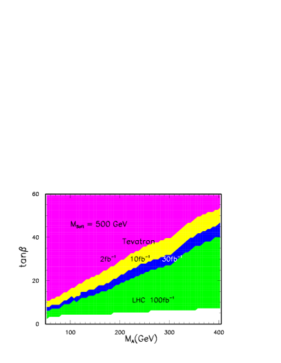
(a)

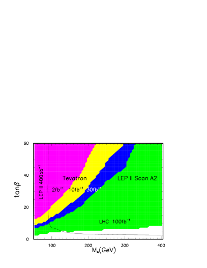
(b)

Figure A.3: $95\%$ C.L. exclusion contours in the $m_{A}$-$\tan\beta$ plane of the MSSM. The areas above the four boundaries are excluded for the Tevatron Run II with the indicated luminosities, and for the LHC with an integrated luminosity of 100 fb^-1. The soft SUSY breaking parameters were chosen uniformly to be 500 GeV in Fig. (a), while the inputs of the “LEP II Scan A2” are used for the Fig. (b) in which LEP II excludes the left area of the solid curve.

To estimate the exclusion regions in the $m_{A}$-$\tan\beta$ plane, a set of soft breaking parameters has to be chosen, which should be compatible with the current data from the LEP II and the Tevatron experiments, while not much larger than 1 TeV. For simplicity, we choose all the soft SUSY breaking parameters (and the Higgs mixing parameter-$\mu$) to be 500 GeV as our “default” values, i.e., $M_{\rm soft}=500$ GeV. In Fig. A.3a, we show the $95\%$ C.L. exclusion contours in the $m_{A}$-$\tan\beta$ plane derived from the measurement of $p\bar{p}/pp\to\phi b\bar{b}\to b\bar{b}b\bar{b}$, using this “default” set of SUSY parameters. The areas above the four boundaries are excluded for the Tevatron Run II with the indicated luminosities, and for the LHC with an integrated luminosity of 100 fb^-1. Needless to say, different choice of SUSY parameters, such as the mass and the mixing of the top squarks and the value (and sign) of the parameter $\mu$, would modify this result. To compare the potential of the Tevatron and the LHC in constraining the MSSM parameters via the $\phi b\bar{b}$ ($\phi=h,A,H$) production to that of the LEP II experiments via $Z\phi$ and $hA$ production, we consider one of the “benchmark” parameter scans discussed in [187, 188], which is called the “LEP II Scan A2”¹² set. For this set of SUSY parameters, the LEP II exclusion contour  [187, 188] at the 95% C.L. is displayed in Fig. A.3b, for a center-of-mass energy of $200$ GeV and an integrated luminosity of $100$ pb^-1 per LEP II experiment. As shown in Fig. A.3b, the Tevatron Run II result, in comparison with the LEP II result, can already cover a substantial region of the parameter space with only a 2 fb^-1 luminosity. Thus, detecting the $\phi b\bar{b}$ signal at hadron colliders can effectively probe the MSSM Higgs sector, especially for models with large $\tan\beta$ values. Furthermore, for $m_{A}\stackrel{{\scriptstyle>}}{{\sim}}100$ GeV, Tevatron Run II is complementary with LEP II, because the latter is not sensitive to that region of parameter space. The LHC can further probe the MSSM down to $\tan\beta\sim$ 7 (15) for $m_{A}<400~{}(1000)$ GeV. This is also shown in Fig. A.4 using the “default” set of SUSY parameters, in which the region above the upper curve is the discovery contour at the $5\sigma$ level for the LHC with an integrated luminosity of 100 fb^-1, and the area above the lower curve can be excluded at $95\%$ C.L., if a signal is not found.

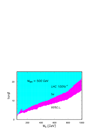
Figure A.4: Discovery and exclusion contours in the $m_{A}$-$\tan\beta$ plane of the MSSM for the LHC with an integrated luminosity of 100 fb^-1. The area above the lower boundary is excluded at $95\%$ C.L., while the upper boundary is the $5\sigma$ discovery contour. The soft SUSY breaking parameters were chosen uniformly to be 500 GeV.

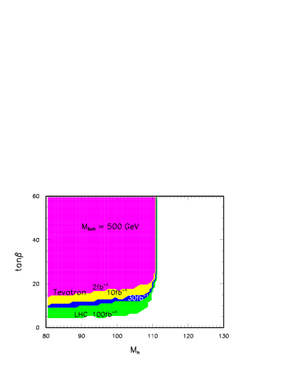
(a)

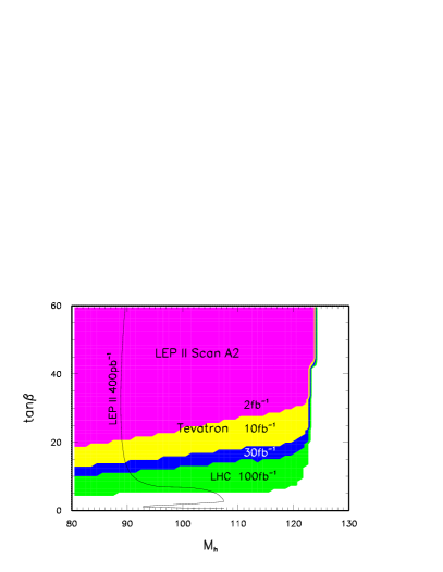
(b)

Figure A.5: $95\%$ C.L. exclusion contours in the $m_{h}$-$\tan\beta$ plane of the MSSM. The areas above the four boundaries are excluded for the Tevatron Run II with the indicated luminosities, and for the LHC with an integrated luminosity of 100 fb^-1. LEP II can exclude the area on the left-hand side of the solid curve in the lower plot.

For completeness, we also present the exclusion contours in the $m_{h}$-$\tan\beta$ and $m_{A}$-$\tan\beta$ planes for both the “default” and the “LEP II Scan A2” sets of SUSY parameters. They are shown in Figs. A.5 and A.6. Again, we see that the Tevatron Run II and the LHC bounds sensitively and complementarily cover the MSSM parameter space in contrast with the LEP II results. We have also studied the bounds with the “LEP II Scan A1” inputs [187, 188] and found that the exclusion contours from the $\phi b\bar{b}$ production are similar to those with “LEP II Scan A2” inputs. The most noticeable difference is that the theoretically allowed range for $m_{h}$ becomes smaller by about 10 GeV in the “Scan A1” set, as compared to the “Scan A2” inputs.

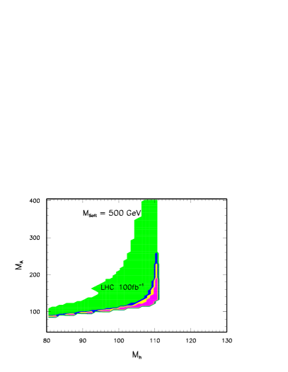
(a)

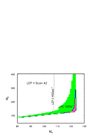
(b)

Figure A.6: $95\%$  C.L. exclusion contours in the $m_{A}$-$m_{h}$ plane of the MSSM. The shaded areas indicate the excluded regions for the Tevatron Run II with integrated luminosities, 2, 10, 30 fb^-1, and for the LHC with an integrated luminosity of 100 fb^-1, as those in the previous figures. LEP II can exclude the area on the left-hand side of the solid curve in the lower plot.

Even though our analyses, described above and in Ref. [182] are quite different from that of Ref. [181], the final bounds at the LHC happen to be in qualitative agreement. We also note that our bounds on the $m_{A}$-$\tan\beta$ plane improve considerably the one obtained in Ref. [189], in which the $p{\bar{p}}\to\phi b\bar{b}\to\tau^{+}\tau^{-}b\bar{b}$ production rate at the Tevatron Run I data was compared to the MSSM prediction. Though, we do not choose to explicitly present projected results for the Tevatron Run I data, we encourage our experimental colleagues to pursue this analysis on the existing Run I data sample, as it seems likely that one could obtain useful information even with the lower luminosity and collider energy of Run I as well as a somewhat lower $b$-tagging efficiency.

Figure A.7: The running of the bottom quark mass $m_{b}(\mu_{R})$ as a function of the renormalization scale $\mu_{R}$. The solid curve shows the QCD evolution alone. The dashed curve further includes the supersymmetric corrections to the “effective” running mass, for $\tan\beta=30$. All soft SUSY breaking parameters have been fixed as $500$ GeV. The dotted curve includes the SUSY corrections but with the sign of the Higgs-mixing parameter $\mu$ flipped.

Before concluding this subsection, we remark upon the effects on our bounds from the possible radiative corrections to the $\phi b\bar{b}$ production process. As mentioned in Sec. II of Ref. [182], one of the dominant correction is from the next-to-leading order (NLO) QCD loops, which are not currently available for the $\phi b\bar{b}$ signal and background cross sections. However, aside from the QCD corrections to the $\phi b\bar{b}$ vertex (part of that can be simply included into the running of the $\phi b\bar{b}$ Yukawa coupling or the running $b$-mass), there are pentagon loops formed by the virtual gluons radiated from an initial state quark (gluon) and re-absorbed by the final state $b$ quark with the $\phi b\bar{b}$ vertex included in the loop. Such QCD corrections are not factorizable so that a consistent improvement of our results is impossible before a full NLO QCD analysis is completed. Putting aside the complexity of the full NLO QCD corrections, we briefly comment upon how the radiative corrections to the running $\phi b\bar{b}$ Yukawa coupling affect our final bounds. At the one-loop level, the relation between the pole quark mass $m_{q}^{\rm pol}$ and the $\overline{\rm MS}$ QCD running mass at the scale $\mu=m_{q}^{\rm pol}$ is:

$$m_{q}(m_{q}^{\rm pol})=m_{q}^{\rm pol}\left[1+\displaystyle\frac{4\alpha_{s}(m_{q}^{\rm pol})}{3\pi}\right]^{-1}~{}.$$ (A.5)

When running upward to any scale $\mu$,

$$m_{q}(\mu)=m_{q}(m_{q}^{\rm pol})\displaystyle\frac{c\left[\alpha_{s}(\mu)/\pi\right]}{c\left[\alpha_{s}(m_{q}^{\rm pol})/\pi\right]}~{},$$ (A.6)

where (cf. Ref. [185])

$$c[x]=(23x/6)^{12/23}\left[1+1.175x\right]~{}~{}{\rm for}~{}~{}m_{b}^{\rm pol}<\mu<m_{t}^{\rm pol},$$

$$c(x)=(7x/2)^{4/7}\left[1+1.398x\right]~{}~{}{\rm for}~{}~{}\mu>m_{t}^{\rm pol}.$$

Numerically, $m_{t}(m_{t}^{\rm pol})\simeq 166$ GeV and $m_{b}(m_{t}^{\rm pol})\simeq 3$ GeV. This QCD correction, Eq.  (A.6), alone will reduce the running mass $m_{b}(\mu)$ by about $40\%$ from the scale $\mu=m_{b}^{\rm pole}\simeq 5$ GeV up to the weak scale of ${\cal O}(200)$ GeV (cf. the solid curve of Fig. A.7). This is however not the full story. The complexity comes from the finite SUSY threshold correction in the large $\tan\beta$ region which are potentially large [192, 193, 194]. As shown in Ref. [193], the dominant one-loop SUSY correction contributes to running $b$-mass a finite term so that $m_{b}(\mu)$ at the SUSY scale $\mu\equiv\mu_{R}=M_{\rm soft}$ is multiplied by a constant factor $~{}1/[1+\Delta_{b}({\rm SUSY})]~{}$, which appears as a common factor in the bottom Yukawa couplings of all three neutral Higgs bosons. For large $\tan\beta$, $\Delta_{b}({\rm SUSY})$ contains the following $\tan\beta$-enhanced terms from sbottom-gluino and stop-chargino loops,

$$\begin{array}[]{l}\Delta_{b}({\rm SUSY})~{}=~{}\displaystyle\left(\frac{\Delta m_{b}}{m_{b}}\right)^{\tilde{b}\tilde{g}}+\left(\frac{\Delta m_{b}}{m_{b}}\right)^{\tilde{t}\tilde{\chi}}\\[12.80365pt] =\displaystyle\frac{-\mu\tan\beta}{16\pi^{2}}\left\{\frac{8}{3}g_{3}^{2}m_{\tilde{g}}F\left(m_{\tilde{b}},m_{\tilde{b}},m_{\tilde{g}}\right)+\left[y_{t}A_{t}F\left(m_{\tilde{t}},m_{\tilde{t}},\mu\right)-g_{2}^{2}M_{2}F\left(m_{\tilde{t}},m_{2},\mu\right)\right]\right\},\end{array}$$ (A.7)

with the function $F$ defined as:

$$F(\sqrt{x},\sqrt{y},\sqrt{z})=-\displaystyle\frac{xy\ln x/y+yz\ln y/z+zx\ln z/x}{(x-y)(y-z)(z-x)}~{}.$$

In these equations, the MSSM Higgs parameter $\mu$ should not be confused with the usual renormalization scale $\mu_{R}$. In (A.7), we have assumed, for simplicity, mass degeneracy for the top and bottom squarks, respectively. Eq. (A.7) shows that the SUSY correction to the running $m_{b}$ is proportional to $\tan\beta$ and $\mu$. Thus, this correction is enhanced for large $\tan\beta$ and non-negligible in comparison with the QCD corrections. Also changing the sign of $\mu$ will vary the sign of the whole correction $\Delta_{b}({\rm SUSY})$ and implies that the SUSY correction can either increase or decrease the running $b$-mass at the energy scale around of ${\cal O}(M_{\rm soft})$. Normally, when defining the running coupling using the Collins-Wilczek-Zee (CWZ) scheme [159], only the $\mu_{R}$-dependent contributions are included while all the $\mu_{R}$-independent terms are absorbed into the corresponding Wilson coefficient functions. However, since the $\mu_{R}$-independent contribution $\Delta_{b}({\rm SUSY})$ is not small for large $\tan\beta$ and a full NLO SUSY calculation is not yet available, we include $\Delta_{b}({\rm SUSY})$ to define an “effective” running coupling/mass of $b$-quark even below the SUSY threshold scale $M_{\rm soft}$. This could give a rough estimate on the large SUSY loop corrections from the $\phi$-$b$-$\bar{b}$ vertex. Obviously, when $\mu_{R}$ is much smaller than $M_{\rm soft}$, the CWZ scheme should be used. Hence, in Fig. A.7, we only show the “effective” running mass $m_{b}(\mu)$ down to about $100$ GeV which is the relevant energy scale and the mass scale ($\sim M_{\rm Higgs}$) considered in this work. Fig. A.7 illustrates that due to the SUSY correction the “effective” running $b$ mass at the weak scale can be either larger or smaller than the SM QCD running value ($\sim 3$ GeV), depending on the choice of the sign of $\mu$ parameter (and also other soft-breaking parameters such as the trilinear coupling $A_{t}$ and masses of the gluino, gaugino, stop and sbottom). For the “default” set of SUSY parameters used in our analysis, all the soft-breaking parameters are set to $500$ GeV for simplicity. It happens to be the case that the SM QCD and SUSY corrections nearly cancel each other so that the “effective” running mass $m_{b}$ is very close to the pole mass value ($\sim 5$ GeV) for the scale above $\sim 100$ GeV (cf. upper curve of Fig. A.7). For comparison, in our analysis using the “LEP II Scan A2” set of SUSY parameters, the SM QCD and SUSY corrections do not cancel and tend to reduce the “effective” running $b$-mass or the Yukawa coupling $y_{b}(\mu)$ which results in a weaker bound for the Tevatron Run II and the LHC, as shown in Fig. A.3b. The difference in the exclusion contours shown in Figs. A.3a and A.3b, derived from the measurement of the $\phi b\bar{b}$ production rate at hadron colliders, is mainly due to the difference in the “effective” running coupling or mass (including the QCD and SUSY corrections), as described above.  We therefore conclude that a full NLO QCD calculation is important for a consistent improvement of our current analysis.

A.2.3 Interpretation of results for Models of soft breaking parameters

The MSSM allows for a very general set of soft SUSY-breaking terms and thus is specified by a large number of free parameters ($\simeq 124$ [179]), though only a complicated subset of this parameter space is consistent with all current experimental results. It is therefore important to understand the mechanism of supersymmetry breaking (which presumably occurs at a high energy scale [195]) and to predict the soft parameters at the weak scale from an underlying model. Many alternative ideas about how supersymmetry might be broken, and how this will result in the low energy soft breaking parameters exist in the literature, including the supergravity inspired (SUGRA) models and gauge-mediated SUSY breaking (GMSB) models. In this section we examine the sensitivity of the $\phi b\bar{b}$ process to probe a few models of SUSY breaking, concentrating for the most part on the popular SUGRA and GMSB models. However, there are also other interesting ideas to which the $\phi b\bar{b}$ process may provide interesting information, because these models naturally prefer a large $\tan\beta$. A few examples include the SO(10) grand unification theories [196] (SO(10) GUTs); the infrared fixed-point scenario [197]; and also a scenario with compositeness, the “more minimal supersymmetric SM” [198].

Supergravity Models with large $\tan\beta$

The supergravity inspired (SUGRA) models [199] incorporate gravity in a natural manner, and solve the problem of SUSY breaking through the introduction of a hidden sector, which breaks SUSY at a very high scale [$\sim{\cal O}(10^{11})$ GeV] and interacts with the MSSM fields only gravitationally. This model offers an exciting glimpse into the possible connection between the heavy top quark and the EWSB by allowing radiative breaking of the electroweak symmetry, in which the large top quark Yukawa coupling can drive one of the Higgs masses negative at energies $\sim m_{Z}$. In the limit of large $\tan\beta$ the bottom and tau Yukawa couplings can also play an important role [200].

Under the assumption that the gravitational interactions are flavor-blind, this model determines the entire SUSY spectrum in terms of five free parameters (at the high energy scale of the SUSY breaking) including a common scalar mass ($\tilde{m}_{0}$), a common gaugino mass ($M$), a common scalar tri-linear interaction term ($A$), $\tan\beta$, and the sign of the Higgs mixing parameter (${\rm sgn}(\mu)$). The weak scale particle spectrum can then be determined by using the renormalization group analysis to run the sparticle masses from the high scale to the weak scale.

Though large $\tan\beta$ is not required by the minimal SUGRA model, it can naturally be accommodated, as demonstrated in [200, 201], where it was found that a large $\tan\beta$ also generally requires that the pseudoscalar Higgs mass be light ($m_{A}\leq$ 200 GeV for $\tan\beta\geq 30$), because the enhanced $b$ and $\tau$ Yukawa couplings act through the renormalization group equations to reduce the down-type Higgs mass term at the weak scale, thus resulting in a light Higgs spectrum. Since the importance of the $b$ and $\tau$ effects in the RG analysis increases with larger $\tan\beta$, as $\tan\beta$ increases the resulting $m_{A}$ decreases, making the large $\tan\beta$ scenario in the SUGRA model particularly easy to probe through the $\phi b\bar{b}$ process. From the limits on the $m_{A}$-$\tan\beta$ plane derived above, it thus seems likely that from the data of the Tevatron Run II with 2 ${\rm fb}^{-1}$ of integrated luminosity, a large portion of the minimal SUGRA model with $\tan\beta\geq 20$ may be excluded.

Gauge-mediated SUSY Breaking Models with Large $\tan\beta$

Models with GMSB break SUSY at a scale which is typically much lower than that present in the SUGRA models. The supersymmetry is generally broken in a hidden sector which directly couples to a set of messenger chiral superfields. This induces a difference in mass between the fermion and scalar components of the messenger fields, which in turn generates masses for the gauginos and sfermions of the MSSM fields via loops involving the ordinary gauge interactions [202, 203]. A generic feature of this scenario is that because of the relatively low scale of SUSY breaking, the gravitino acquires a much smaller mass than in the SUGRA scenarios, and is generally the lightest supersymmetric partner (LSP). While specific models of GMSB vary as to their assumptions and relevant parameters, generally what must be assumed is the field content of the messenger sector (including transformation properties under the gauge group and number of multiplets in the theory) and the scale at which SUSY is broken in the hidden sector.

The minimal GMSB models can also result in a radiative breaking of the EWSB, through the renormalization group evolution of the Higgs masses (driven by the large top Yukawa coupling) from the effective SUSY breaking scale to the weak scale. As in the SUGRA model case, this evolution can drive the mass term of the up-type Higgs negative at the weak scale, thus breaking the electroweak symmetry. In fact, because the effective SUSY breaking scale in a GMSB model is typically much lower than in the SUGRA model (and thus closer to the weak scale), in order for the proper EWSB to occur, it was demonstrated in [204] that a large $\tan\beta$ is required (about $30$-$40$). However, because the effective SUSY breaking scale is typically much lower than in the SUGRA model, the large effects of the $b$ and $\tau$ on the Higgs mass running do not reduce the Higgs spectrum to the degree that occurs in the SUGRA model with large $\tan\beta$, and thus result in a heavier $A$ with mass of about 400 GeV. So, this particular model would only be explored through the $\phi b\bar{b}$ process at the LHC. However, more general analyses of the GMSB scenario [205, 206, 207, 208], introducing more degrees of freedom in the messenger sector than the minimal model, can allow for large $\tan\beta$ and relax $m_{A}$ to be as low as about 200 GeV. Thus, through the $\phi b\bar{b}$ production these more general models can be first probed at the Tevatron for the relevant mass range, and then largely explored at the LHC.

A.3 Conclusions

It remains a challenging task to determine the underlying dynamics of the electroweak symmetry breaking and the flavor symmetry breaking. Either fundamental or composite Higgs boson(s) may play a central role in the mass generation of the weak gauge bosons and the fermions. The heavy top quark, with a mass on the same order as the scale of the electroweak symmetry breaking, suggests that the top quark may play a special role in the mechanism of mass generation. In this work, we have shown that in the typical models of this type, the bottom quark, as the weak isospin partner of the top quark, can also participate in the dynamics of mass generation, and serves as an effective probe of the possible new physics associated with the Higgs and top sectors.

We have presented a model-independent analysis on Higgs boson production in association with bottom quarks, via the reaction $p\bar{p}/pp\to\phi b\bar{b}\to b\bar{b}b\bar{b}$, at the Tevatron Run II and the LHC. Using the complete tree level calculation with an estimated QCD $k$-factor of 2, we derive the exclusion contour for the enhancement factor (in the coupling of $\phi b\bar{b}$ relative to that of the SM) versus the Higgs mass $m_{\phi}$ at the $95\%$ C.L., assuming a signal is not found.

We apply these results to analyze the constraints on the parameter space of the MSSM (in the large $\tan\beta$ region) with naturally large bottom Yukawa couplings. To confirm the MSSM, it is necessary to detect all the predicted neutral Higgs bosons $h,~{}H,~{}A$ and the charged scalars $H^{\pm}$. From LEP II, depending on the choice of the MSSM soft-breaking parameters, the current $95\%$ C.L. bounds on the masses of the MSSM Higgs bosons are about 70 GeV for both the $CP$-even scalar $h$ and the $CP$-odd scalar $A$ [209]. It can be improved at LEP II with higher luminosity and maximal energy, but the bounds on the Higgs masses will not be much larger than $\sim m_{Z}$ for an arbitrary $\tan\beta$ value. The $Wh$ and $WH$ associated production at the Tevatron Run II can further improve these bounds, if a signal is not observed. At the LHC, a large portion of parameter space can be tested via $pp\to t\bar{t}+h(\to\gamma\gamma)+X$, and $pp\to h(\to ZZ^{\ast})+X$, etc. [210, 211]. A future high energy $e^{+}e^{-}$ collider will fully test the MSSM Higgs sector [212, 213] through the reactions $e^{+}e^{-}\to Z+h(H),\,A+h(H),\,H^{+}H^{-}$, etc. In this work, we demonstrate that studying the $\phi b\bar{b}$ channel at hadron colliders can further improve our knowledge on MSSM. The exclusion contours on the $m_{A}$-$\tan\beta$ plane of the MSSM shows that the Tevatron and the LHC are sensitive to a large portion of the parameter space via this mode. It therefore provides a complementary probe of the MSSM Higgs sector in comparison with that from LEP II. The implications of these bounds in the parameter space on both the supergravity and the gauge-mediated SUSY breaking models are further discussed. We find that the $\phi b\bar{b}$ process can effectively test the models with either scheme of the SUSY soft-breaking in the large $\tan\beta$ scenario.

In conclusion, the stringent constraints obtained by studying the associated $\phi b\bar{b}$ production at hadron colliders for the supersymmetric models show the utility of this search mode. However, much work remains to be done. For example, we have found that a $b$-trigger is essential for this analysis. In fact, the CDF group at the Fermilab has demonstrated that it is possible to detect events with four or more jets and two or more $b$-tags [214], which can significantly be improved with the implementation of $b$-trigger at the Run II of the Tevatron [215]. However, the large QCD 4-jet background rate at the LHC can potentially make triggering on the $b{\bar{b}}\phi(\rightarrow b{\bar{b}})$ events difficult, though it is expected that $b$-trigger would becomes more efficient for a heavier (pseudo-)scalar $\phi$. (This is because the $b$-jets from the decay of a heavier $\phi$ are more energetic, and its QCD background rate drops rapidly as a function of the transverse momentum of the triggered jet.) We hope that the interesting results afforded by studying this channel will stimulate interest in working on these problems in our experimental colleagues.

We have found that the $\phi b\bar{b}$ process complements Higgs searches in other channels, and thus it is expected that experimental searches for this signature at the Tevatron Run II (and possibly beyond) and the CERN LHC will provide interesting and important information about the mechanism of the electroweak symmetry breaking and the fermion mass generation.

Appendix B “Intrinsic $k_{T}$” and Soft Gluon Resummation

B.1 Introduction

For many years, it has been a common practice to “smear” the transverse momentum ($p_{T}$) distribution of the Drell-Yan pairs or the direct photons calculated in perturbative QCD to obtain a better agreement between the theoretical predictions and the experimental data. The argument of smearing the $p_{T}$ distribution is that any parton inside a hadron generally has a non-zero transverse momentum which is called the “intrinsic transverse momentum” (or “intrinsic $k_{T}$”) of the parton. The concept of intrinsic transverse momentum evolved in the literature from the covariant parton model of Landshoff, Polkinghorne and Short [216] to the $k_{T}$ dependent parton distributions of Collins and Soper [217]. Intrinsic $k_{T}$ emerges from the Fermi motion of partons within the hadron. Since the Fermi motion is uncorrelated with the direction of the acceleration, it leads to momentum fluctuations in the transverse directions. By definition, this ab initio transverse momentum has a non-perturbative nature and typically is of the order of $\Lambda_{QCD}$, i.e. a few hundred MeV. It was however found that the amount of “smearing” needed to make the theoretical prediction of the $p_{T}$ distribution agree with data in some cases could be as large as a few GeV which is much larger than $\Lambda_{QCD}$. To understand this, we need the full armory of QCD including both the perturbative and the non-perturbative part. In the low $p_{T}$ region, which is the region where a perturbative calculation will deviate the most from experimental data, one needs to take into account the effects of multiple (soft and collinear) gluon radiation from both the initial and the final states. For extremely low $p_{T}$ regions, the non-perturbative effects of the QCD theory, e.g. effects due to higher twist operators, should also be included when comparing with the measurements. In this work we make use of the soft gluon resummation formalism developed by Collins and Soper to estimate the amount of smearing needed to apply onto a perturbative QCD calculation so that its prediction would agrees with that from a resummation calculation.

For the Drell-Yan process, in which only the initial state involves QCD colors, Collins, Soper and Sterman (CSS) gave a set of comprehensive formula to account for the effects on the $p_{T}$ distribution of the lepton pair due to the multiple soft (and collinear) gluon emissions in the initial state. In the CSS formalism, the perturbative part of the multiple gluon radiation effects is summarized by the perturbative Sudakov form factor and some Wilson coefficients (i.e. $C$-functions); the non-perturbative part of QCD physics which is relevant to the low $p_{T}$ distribution is parametrized by some non-perturbative functions which at the present time can only be fitted to some existing Drell-Yan data. The moral is that if the CSS formalism is the correct parametrization of the multiple gluon effects, then the same form of the non-perturbative functions (fitted to particular sets of data) should also be applied to the other Drell-Yan data at different energies of the colliders and/or invariant masses of the lepton pairs.

The effects due to initial state gluon radiations should be universal to any process involving the same kinds of incoming partons with similar QCD color structures in the events. As we saw earlier, the CSS formalism describes well the transverse momentum distribution of $W^{\pm}$, $Z$-bosons and diphotons at the Tevatron. Although the direct photon process does not have the same kinds of incoming partons or color structures as those contributing to the Drell-Yan process, we expect that the dominant effects on the low $p_{T}$ distribution of the direct photon would come from the initial state radiation whose non-perturbative contributions are more or less the same as those measured in the Drell-Yan process. As far as we know, there is no proof for this statement. It is only our educated guess that the non-perturbative behavior of the partons inside a hadron would be similar. Of course, the calculable perturbative Sudakov form factors would distinguish an initial gluon parton from an initial quark (or anti-quark) parton, and should be properly included in the CSS formalism for calculating the $p_{T}$ distributions. Although we lack theoretical proof, there are indications from phenomenology which seem to confirm the need of the resummation of the initial state QCD radiation for the direct photon process for low $p_{T}$. Monte Carlo simulations (using Bauer-Reno’s MC or PYTHIA) indicate that initial state radiation improves the finite order QCD results. There are also efforts to derive CSS type formulas with partial success.

In this work, we do not intend to do a complete calculation on the $p_{T}$ distribution of the direct photon using the CSS formalism, which as described in the above, involves both the perturbative Sudakov form factor and the non-perturbative functions. We only apply the non-perturbative part of the CSS formalism to explain the amount of $p_{T}$-smearing needed to make a “smeared” next-to-leading order (NLO) QCD perturbative calculation agree with the experimental data of the direct photon in its transverse momentum distribution. We show that for the low energy fixed-target experiments, the non-perturbative part of the CSS resummation formalism alone can explain the required amount of low-$p_{T}$-smearing. However, to explain the high energy collider data, such as those at the Tevatron, the perturbative part of the Sudakov form factor should also be included in the calculation. We defer the complete calculation, which separately includes the effects from the perturbative Sudakov form factor associated with $qq$ ($q{\bar{q}}$) or $gq$ ($g{\bar{q}}$) initiated direct photon production processes, to our future work.

B.2 Smearing $p_{T}$ Distributions of Direct Photons

In this section we show that it is possible to resolve the discrepancy between the theoretical prediction and the experimental data of the $p_{T}$ distribution of the direct photon measured in fixed target experiments. This is achieved by applying the CSS resummation formalism and by including only the contribution from the non-perturbative functions of the formalism, which (in the direct photon context) has just one free parameter to be determined by experimental data. Our approach is to assume the approximative universality (i.e. insensitivity to the flavors of the active partons) of the non-perturbative function in the CSS resummation. Hence, the same non-perturbative function that is used to describe the Drell-Yan process can also be used for the direct photon production to improve the next-to-leading order predictions. What follows in this section is rather intuitive and is not backed up by full theoretical understanding or precise calculations.

It is a fact that the transverse momentum distribution of the photons produced directly at hadron-hadron collisions deviates systematically from the experimental measurement. The NLO QCD calculations [218] give less steep curves than the experimental data. A recent global analysis of the problem [219], examining both fixed target and collider experiments, concluded that neither new parton distributions nor new fragmentation functions can resolve the problem, since the deviation occurs at different $x$ values in experiments with different energies. In the above study the authors also exclude the possibility that the deviation can be entirely accounted for the scale choice in the calculations.

It was shown in Ref. [219] that convoluting the theoretical $p_{T}$ distribution with a Gaussian resolution function can raise the cross section at the low $p_{T}$ end so that it agrees with the experimental data better. This is because smearing a falling distribution by a Gaussian can steepen its original shape. Writing the smeared $p_{T}$ distribution as

$${d\sigma\over dp_{T}}={1\over\Delta\sqrt{\pi/2}}\int_{-\infty}^{\infty}dp_{T}^{\prime}{d\sigma^{NLO}\over dp_{T}^{\prime}}~{}{\rm e}^{-(p_{T}-p_{T}^{\prime})^{2}/2\Delta^{2}}$$ (B.1)

defines $\Delta$ as the quantitative measure of the smearing. The amount of the smearing needed differs for different center of mass energies (see the first and second columns of Table B.1).

There are several puzzling details here. First, there is no theoretical reason to introduce an ad hoc smearing of the NLO results. Secondly, the amount of the intrinsic $k_{T}$ that the partons acquire because of the Fermi motion within the hadron is in the order of $\Lambda_{QCD}$, which is a few hundred MeV. The amount of smearing that brings theory and experiment to agreement is more than that. Finally, even if one invents a mechanism to introduce some type of a smearing, one has to find a smearing function that has a dependence on $S$ which is the square of the center of mass energy of the hadron-hadron collision, and make sure that the smearing does not ruin the agreement at higher $p_{T}$’s.

To overcome all the above difficulties we propose the application of the non-perturbative function of the CSS resummation as a smearing device. This simple idea seems to be plausible because the non-perturbative function has a Gaussian form and depends on the center of mass energy of the process. Although we do not have a proof, after noticing that the non-perturbative function acts like a smearing factor at the Drell-Yan process (for details see the next section), we may as well try it at the direct photon process.

The non-perturbative function is usually parametrized in a simple Gaussian form:

$$W^{NP}(Q_{T},Q,Q_{0})={1\over 2G_{2}(Q,Q_{0})}\exp{\left\{-Q_{T}^{2}/4G_{2}(Q,Q_{0})\right\}},$$ (B.2)

with $G_{2}(Q,Q_{0})=g_{1}+g_{2}\ln({Q/2Q_{0}})$, $g_{1}=0.11\,{\rm GeV}^{2}$, $g_{2}=0.58\,{\rm GeV}^{2}$ and $Q_{0}=1.6\,{\rm GeV}$. We can easily check whether the amount of the smearing from the non-perturbative function comes close to what phenomenology demands. First we substitute $\sqrt{Sx^{2}}$ for $Q$ in $G_{2}(Q,Q_{0})$. This substitution is inspired by the relation $Q=\sqrt{Sx_{A}x_{B}}=\sqrt{\hat{s}}$ that holds in the case of the Drell-Yan process, with $\sqrt{S}$ being the center of mass energy of the colliding hadrons, and $x_{A}$, $x_{B}$ the longitudinal momentum fractions of the incoming partons. Since these latter quantities are not measured at the direct photon production we take $x$ as a free parameter and let data determine its value. The best fit to the fixed target experimental data gives $x=0.3$. Now we can calculate the numerical value of $G_{2}(Q,Q_{0})$ for the six different experiment. The results are shown in the last column of Table B.1.

Experiment	$\sqrt{S}$ (GeV)	$\Delta$ (GeV)	$\sqrt{2G(Q,Q_{0})}$ (GeV)
WA70	23	${\ \lower-1.2pt\vbox{\hbox{\hbox to0.0pt{$<$\hss}\lower 5.0pt\vbox{\hbox{$\sim$}}}}\ }1$	1.0
UA6	24	${\ \lower-1.2pt\vbox{\hbox{\hbox to0.0pt{$<$\hss}\lower 5.0pt\vbox{\hbox{$\sim$}}}}\ }1$	1.1
E706	31	1-2	1.2
R806	63	2-3	1.5
UA2	630	3-4	2.2
CDF	1800	3-4	2.5

Table B.1: The amount of the smearing needed and the amount provided by the non-perturbative function to make theory agree with experiment for different direct photon experiments. Values of $\Delta$ are taken from Ref. [4].

We see at first sight that the non-perturbative function provides about the right amount of smearing needed to bring the theory prediction and the experimental data in a better agreement. Examining Table B.1 more closely, we observe that the smearing from the non-perturbative function falls short as the center of mass energy of the collider increases. Hence, for the fixed target experiments at a higher energy and for the collider experiments, the contribution from the non-perturbative function alone cannot account for all the amount of smearing needed.

This can also be seen from Fig. B.1. Substituting the non-perturbative function into the convolution equation (B.1), the theoretical distributions can be rendered close to the experimental ones as it is shown in Fig. B.1. (Among the fixed target experiments, UA6 $p\overline{p}$ data are not shown, but they have the same characteristics as UA6 $pp$ data.) The NLO QCD curve is shown in short dashes. The long dashed curve is the convolution of the theory with the non-perturbative function. As anticipated, the agreement between the data and the theoretical prediction improves in low the $p_{T}$ region after including the smearing effects for all the low energy fixed target experiments. However, the convolution (i.e. the $p_{T}$-smearing) is less effective for the collider data (not shown). As discussed above, at collider energies the perturbative Sudakov form factor arising from resumming over the large logs which are due to the initial state radiation will be important besides the non-perturbative effects, and it is not included in the present study.

Figure B.1: Experiment numbers are listed at the top of each plot. Short dashed line: NLO transverse momentum distribution. Long dashed line: NLO theory convoluted with the Fourier transform of the non-perturbative function used in the Drell-Yan resummation formalism.

In conclusion, the above results suggest that there is an important similarity between the Drell-Yan and the direct photon processes. The roots of this correspondence are found in the initial state radiation, which is present in both cases.

B.3 $p_{T}$-Smearing and Soft gluon Resummation

In this section we demonstrate that “$p_{T}$-smearing” naturally arises within the resummation formalism of Collins, Soper and Sterman [44, 45, 46]. It is the same type of smearing that is needed to make the theoretical prediction agree with the experimental data in $p_{T}$ distribution of the direct photon produced in fixed target experiments.

The canonical example of the CSS formalism is the hadronic production of electroweak vector bosons. In the Drell-Yan type of process the kinematical variables of the vector boson $V$ (real or virtual) are selected to be its invariant mass $Q$, rapidity $y$, transverse momentum $Q_{T}$, and azimuthal angle $\phi_{V}$, measured in the laboratory frame. The kinematics of the leptons from the decay of the vector boson can be described by the polar angle $\theta$ and the azimuthal angle $\phi$, defined in the Collins-Soper frame [52]. The fully differential cross section of the vector boson production and decay is given by the resummation formula:

$$\left({d\sigma(AB\rightarrow V(\rightarrow{l{\bar{l}^{\prime}}})X)\over dQ^{2}\,dy\,dQ^{2}_{T}\,d\phi_{V}\,d\cos{\theta}\,d\phi}\right)_{res}={1\over 96\pi^{2}S}\,{Q^{2}\over(Q^{2}-M_{V}^{2})^{2}+M_{V}^{2}\Gamma_{V}^{2}}$$

$$~{}~{}\times\bigg{\{}{1\over(2\pi)^{2}}\int d^{2}b\,e^{i{\vec{Q}_{T}}\cdot{\vec{b}}}\,\sum_{j,k}{\widetilde{W}_{jk}(b_{*},Q,x_{A},x_{B},\theta,\phi)}\,W^{NP}_{jk}(b,Q,x_{A},x_{B})$$

$$~{}~{}~{}~{}+~{}Y(Q_{T},Q,x_{A},x_{B},\theta,\phi)\bigg{\}}.$$ (B.3)

Here

$$\widetilde{W}_{jk}(b,Q,x_{A},x_{B},\theta,\phi)=\widetilde{w}_{jk}(x_{A},x_{B},\theta,\phi)\exp{\left\{-S(b,Q)\right\}},$$ (B.4)

with the Sudakov exponent

$$S(b,Q)=\int_{b_{0}^{2}/b^{2}}^{Q^{2}}{d{\bar{\mu}}^{2}\over{\bar{\mu}}^{2}}\left[\ln\left({Q^{2}\over{\bar{\mu}}^{2}}\right)A\big{(}\alpha_{s}({\bar{\mu}})\big{)}+B\big{(}\alpha_{s}({\bar{\mu}})\big{)}\right],$$ (B.5)

and $x_{A,B}=\sqrt{Q}\exp{\left(\pm y\right)}$. In the above expressions $j$ represents quark flavors and $\bar{k}$ stands for anti-quark flavors. The definition of $\widetilde{w}$ together with further details can be found in Chapter 2.

In Eq. (B.3), the impact parameter $b$ is to be integrated from 0 to $\infty$. However, for $b$ larger than a certain $b_{max}$, corresponding to energy scales less than $1/b_{max}$, the QCD coupling $\alpha_{s}$ becomes so large that a perturbative calculation is no longer reliable. To avoid this, $\widetilde{W}$ is evaluated at $b_{*}$, with

$$b_{*}={b\over\sqrt{1+(b/b_{max})^{2}}}$$ (B.6)

such that $b_{*}$ never exceeds $b_{max}$. Thus $b_{max}$ is the theoretical scale that separates perturbative and non-perturbative physics in the resummation formalism. Just like other theoretical scales (e.g. renormalization or factorization scales), $b_{max}$ defines a somewhat arbitrary separation. Choosing $b_{max}=1/2$ GeV^-1 (as usual) instead of $1/\Lambda_{QCD}$ shuffles parts of the low $Q_{T}$ perturbative physics related to the initial state radiation into the non-perturbative function. Thus the non-perturbative function contains more than just the intrinsic partonic $k_{T}$. $W^{NP}$ is needed in the formalism in order to suppress the contribution of $\widetilde{W}_{jk}$ from the large $b$ (small $Q_{T}$) region and to parametrize our ignorance of the non-perturbative phenomenon there. Furthermore, since physics cannot depend on $b_{max}$, $W^{NP}$ carries an implicit $b_{max}$ dependence through the non-perturbative parameters $g_{i}$ defined below. Generally $W^{NP}$ has the structure

$$W^{NP}_{jk}(b,Q,Q_{0},x_{A},x_{B})=\exp{\left\{-S^{NP}(b,Q,Q_{0},x_{A},x_{B})\right\}},$$ (B.7)

with the non-perturbative exponent

$$S^{NP}(b,Q,Q_{0},x_{A},x_{B})=h_{1}(b)\ln\left(Q^{2}\over Q^{2}_{0}\right)+h_{j/A}(x_{A},b)+h_{{\bar{k}}/B}(x_{B},b).$$ (B.8)

Here $h_{1}$, $h_{j/A}$ and $h_{{\bar{k}}/B}$ cannot be calculated using perturbation theory, they must be determined using experimental data. The form of the non-perturbative exponent $S^{NP}$ is inspired by the form of the Sudakov form factor which in turn is derived by renormalization group arguments discussed in Chapter 2. Since for large values of the impact parameter the non-perturbative function has to cancel the contribution of $\widetilde{W}$, the structure of the non-perturbative exponent is determined by the Sudakov exponent, that is, by perturbative resummation physics.

We restrict our attention to the small $Q_{T}$ region, where resummation effects may be important and are detectable. In the $Q_{T}^{2}\ll Q^{2}$ region the $Y$-term in Eq. (B.3) is negligible. Dropping the $Y$ piece and rewriting $\widetilde{W}_{jk}$ in a form of a Fourier transform we obtain

$$\left({d\sigma(AB\rightarrow V(\rightarrow{l{\bar{l}^{\prime}}})X)\over dQ^{2}\,dy\,dQ^{2}_{T}\,d\phi_{V}\,d\cos{\theta}\,d\phi}\right)_{res-Y}={1\over 96\pi^{2}S}\,{Q^{2}\over(Q^{2}-M_{V}^{2})^{2}+M_{V}^{2}\Gamma_{V}^{2}}$$

$$~{}~{}\times\bigg{\{}{1\over(2\pi)^{2}}\int d^{2}b\,e^{i{\vec{Q}_{T}}\cdot{\vec{b}}}\,\sum_{j,k}\left({1\over 2\pi}\int d^{2}Q_{T}^{\prime}\,e^{-i{\vec{Q}_{T}^{\prime}}\cdot{\vec{b}}}\,{\widetilde{W}_{jk}(Q_{T}^{\prime},Q,x_{A},x_{B},\theta,\phi)}\right)$$

$$~{}~{}~{}~{}~{}~{}~{}~{}~{}~{}~{}~{}~{}~{}~{}~{}~{}~{}~{}~{}~{}~{}~{}~{}~{}~{}~{}~{}~{}~{}~{}\times~{}W^{NP}_{jk}(b,Q,x_{A},x_{B})\bigg{\}}$$ (B.9)

The $b$ integral can formally be carried out, resulting in the appearance of the inverse Fourier transform of the non-perturbative function. Introducing the convolution notation for the remaining integral, the first part of the resummation formula in $Q_{T}$ space simplifies to

$$\left({d\sigma(AB\rightarrow V(\rightarrow{l{\bar{l}^{\prime}}})X)\over dQ^{2}\,dy\,dQ^{2}_{T}\,d\phi_{V}\,d\cos{\theta}\,d\phi}\right)_{res-Y}={1\over 96\pi^{2}S}\,{Q^{2}\over(Q^{2}-M_{V}^{2})^{2}+M_{V}^{2}\Gamma_{V}^{2}}$$

$$~{}~{}\times{1\over(2\pi)^{2}}\left(\widetilde{W}_{jk}\otimes~{}W^{NP}_{jk}\right)(Q_{T},Q,x_{A},x_{B},\theta,\phi)$$ (B.10)

where $\otimes$ denotes the convolution and is defined by

$$\left(\widetilde{W}_{jk}\otimes~{}W^{NP}_{jk}\right)(Q_{T},Q,x_{A},x_{B},\theta,\phi)=$$

$$~{}~{}~{}~{}\sum_{j,k}\int d^{2}Q_{T}^{\prime}\,\widetilde{W}_{jk}(Q_{T}^{\prime},Q,x_{A},x_{B},\theta,\phi)\,W^{NP}_{jk}(Q_{T}-Q_{T}^{\prime},Q,x_{A},x_{B}).$$ (B.11)

Eq. (B.10) expresses that the resummed cross section at low $Q_{T}$ region is given by the convolution of the exponentiated singular part of the hard scattering cross section with the non-perturbative function. It can be viewed as if the hard cross section were smeared by the non-perturbative function.

The non-perturbative function is approximated with the flavor independent, Gaussian parametrization [73, 72]

$$S^{NP}(b,Q,Q_{0},x_{A},x_{B})=G_{1}(x_{A},x_{B})b+G_{2}(Q,Q_{0})b^{2}~{}~{}~{}{\rm with}$$

$$G_{1}=g_{1}g_{3}\ln{(100x_{A}x_{B})}~{}~{}~{}\rm{and}~{}~{}~{}G_{2}=g_{1}+g_{2}\ln\left({Q\over 2Q_{0}}\right)$$ (B.12)

Recent analysis gives $g_{1}=0.11\,{\rm GeV}^{2}$, $g_{2}=0.58\,{\rm GeV}^{2}$ , $g_{3}=-1.5\,{\rm GeV}^{-1}$ and $Q_{0}=1.6\,{\rm GeV}$ [73]. The Fourier transform of the above non-perturbative function (for simplicity taken without the linear term) is

$$W^{NP}(Q_{T},Q,Q_{0})={1\over 2G_{2}(Q,Q_{0})}\exp{\left\{-Q_{T}^{2}/4G_{2}(Q,Q_{0})\right\}}.$$ (B.13)

This is the form that we used to smear the direct photon NLO distribution.

The resummation formula (B.10) indicates that the effect of resumming the initial state soft gluon radiations is twofold. First, it exponentiates contributions that are singular as $Q_{T}\rightarrow 0$ and therefore contain large logs ($\ln(Q/Q_{T})$) of the finite order cross section, into the Sudakov form factor $\exp(-S)$. Second, it smears the above perturbative Sudakov form factor with the non-perturbative function $W^{NP}$. The amount of the smearing provided by the non-perturbative function is larger than the amount of the intrinsic $k_{T}$ because the non-perturbative function contains parts of the perturbative multiple soft gluon emission effects in the low $Q_{T}$ region. Note that the separation between the perturbative Sudakov form factor and the non-perturbative function depends on the arbitrary parameter $b_{max}$ used in the CSS formalism. Hence, the non-perturbative function also contains some perturbative physics.

We expect a similar underlying mechanism of the initial state radiation to be present in the direct photon process. That would alter the shape of the transverse momentum distribution of the direct photon in the low $p_{T}$ region. This is proven in the agreement between the experimental data and the predicted low-$p_{T}$ distribution after including the smearing effects due to the non-perturbative part of the CSS resummation formalism. For the direct photon process, however, the color flow of the initial state partons is different from that for the Drell-Yan process. This slightly complicates the above resummation results and affects the non-perturbative function given above. Even though, for example, the value of the $g_{i}$ parameters may change, the form of the non-perturbative function should be the same. Our phenomenological parameter $x$ partly accounts for these changes.

At low energies, due to lack of phase space, the multi gluon initial state radiation is suppressed. Mathematically this means that the contribution of the perturbative Sudakov form factor is less important. In the low energy region, expansion of $\widetilde{W}$ in term of $\alpha_{s}$ can be approximated by the first few terms, since $\ln(Q/Q_{T})$ will not be large. (The two characteristic scales $Q_{T}$ and $Q$ are of the same order in magnitude.) The first few terms in the expansion of $\widetilde{W}$ are the singular parts of the fixed order cross section, which dominate the low $Q_{T}$ behavior. In the CSS resummation formalism, this singular part is smeared by the non-perturbative function. This suggests that one can improve the theoretical prediction of a fixed order perturbative calculation at the low $p_{T}$ region by smearing it with the non-perturbative function described above. This is indeed what we see in Table 1 for low energy fixed target data.

According to the resummation formula (B.3) the effect of the non-perturbative function on $\widetilde{W}$ is larger at the low $Q_{T}$ (large $b$) end. As $Q_{T}$ increases ($b$ decreases) the non-perturbative function approaches unity. The Sudakov form factor, on the other hand, increases its contribution with increasing $Q_{T}$ (decreasing $b$), which becomes evident after expanding it in $\alpha_{s}$:

$$S(b,Q)=\frac{\alpha_{s}}{\pi}\ln\left(\frac{bQ}{b_{0}}\right)\left[A_{1}\ln\left(\frac{bQ}{b_{0}}\right)+B_{1}\right]+{\cal O}(\alpha_{s}^{2}).$$ (B.14)

This means that at higher direct photon $p_{T}$ region the effect of the Sudakov factor would also be important. This effect might just cancel the smearing effect of the non-perturbative function leaving the higher $p_{T}$ data virtually unchanged, which would explain why $k_{T}$ smearing has to be performed only in the lowest $p_{T}$ regions.

For data from experiments with higher center of mass energies, the initial state multiple gluon radiation effects are important. This also means that the perturbative Sudakov form factor is important. In this case, the full resummation calculations should be carried out to describe the $p_{T}$ distribution of the direct photon produced at high energy hadron colliders, such as the Tevatron. For a rough estimate of the effect of a Sudakov type of form factor at high energy direct photon experiments we turn to the resummation formula again. We observe that writing (B.3) into a form of a convolution can be repeated grouping terms in a slightly different way. Taking the Sudakov factor out from $\widetilde{W}$ and putting it into $W^{NP}$, the argument that leads to the convolution form (B.10) can be repeated without a change. Now that the smearing function contains the Sudakov part we ask the question, whether this effective smearing function has a broader width, that is whether it provides an additional smearing what the collider experiments need. To answer this we have to evaluate the (two dimensional) Fourier transform of the non-perturbative function multiplied with the Sudakov factor evaluated at $b_{*}$. The simplest way of doing this is to perform the integrations numerically. The result agrees with our expectations. The effective smearing function has an approximate Gaussian shape and a width $\Delta_{eff}$ larger than of the non-perturbative function, with the increase depending on the center of mass energy. We can interpret this result as an indication that the missing $p_{T}$ smearing may well come from the Sudakov form factor.

To further illustrate the power of the Fourier transformed form of the resummation formula, we attempt some simple estimates on observables that are related to the transverse momentum of the $W$-boson in hadron collisions. Consider the average transverse momentum $\left\langle Q_{T}\right\rangle$ of the weak vector boson produced in hadron collisions. Inserting the Fourier transform (B.13) of the non-perturbative function into formula (B.10) the only $Q_{T}$ dependence of the right hand side comes from the exponential term of the non-perturbative function $\exp({-(Q_{T}-Q_{T}^{\prime})^{2}/4G)}$. Since the largest contribution in the $Q_{T}^{\prime}$ integral comes from the region where $Q_{T}^{\prime}\sim Q_{T}$ we approximate the $Q_{T}^{\prime}{}^{2}$ term by $Q_{T}^{2}$. To calculate the average transverse momentum we make use of the integral

$$\int_{0}^{+\infty}dQ_{T}^{\prime}\,Q_{T}^{\prime}\exp\left\{Q_{T}^{\prime}Q_{T}/2G_{2}\right\}={4G_{2}^{2}\over Q_{T}^{2}}.$$ (B.15)

Under the above approximations we obtain that the average $Q_{T}$ is proportional to $G_{2}(Q,Q_{0})$. (A more elaborate numerical calculation supports this.) The result is given on Fig. B.2a. We find that the average $Q_{T}$ grows as log of $Q$.

Figure B.2: a) The invariant mass versus the average $W^{\pm}$ boson transverse momentum in the resummed calculation. b) The center of mass energy versus the average $W^{\pm}$ boson transverse momentum in the resummed calculation.

Using the first order equality $Q=\sqrt{Sx_{A}x_{B}}$ we can obtain a similar conclusion for the dependence of the average transverse momentum on the center of mass energy of the hadron colliders. Of course, the $S$ dependence will not be purely logarithmic, since $\widetilde{W}_{jk}$ (and a more thorough parametrization of the non-perturbative function) makes it more complicated. Nevertheless, as Fig. B.2b shows, even the $S$ dependence of $\left\langle Q_{T}\right\rangle$ is not very far from being logarithmic. This result differs from what one would infer from a finite order perturbative calculation which would predict that $\left\langle Q_{T}\right\rangle$ is proportional to $E_{cm}=\sqrt{S}$.

In conclusion, we have shown that the discrepancy between the theoretical prediction and the experimental data of the $p_{T}$ distribution of the direct photon can be resolved for the fixed target experiments after smearing the NLO calculation by the non-perturbative function that is suggested by the CSS resummation formalism. To improve the phenomenological method described in this work for high energy collider experiments, one needs to include the effects on $p_{T}$ distribution of direct photons from the perturbative Sudakov form factor in the CSS resummation formalism.

Bibliography

- [1] F.J. Dyson, Field Theory, reproduced in Particles and Fields, Scientific American 17 (1980).
-
[2]
S. Weinberg,
Phys. Rev. Lett. 19, 1264 (1967);
Phys. Rev. D 5, 1412 (1972);
A. Salam, in
Nobel Symposium No. 8,
edited by N. Svartholm, Almqvist and Wiksell, Stockholm, 1968;
S. Glashow,
Nucl. Phys. 22, 579 (1961);
D. J. Gross and F. Wilczek,
Phys. Rev. D 8, 3633 (1973);
Phys. Rev. D 9, 908 (1974);
H.D. Politzer,
Phys. Rept. 14, 129 (1974);
For introductory texts on the Standard Model see:
F. Halzen and A.D. Martin, Quarks and Leptons: An Introductory Course in Modern Particle Physics, John Wiley & Sons, Inc., (1984); T.-P. Cheng and L.-F. Li, Gauge theory of Elementary Particle Physics, Oxford University Press, Oxford, England, (1984); G. Kane, Modern Elementary Particle Physics, Addison-Wesley, Inc., (1987); J.F. Donoghue, E. Golowich and B. R. Holstein, Dynamics of the Standard Model, Cambridge University Press, (1992). - [3] Particle Data Group (C. Caso et al.), “Review of Particle Physics”, The European Physical Journal C 3, 1 (1998).
- [4] P. Ramond, Field Theory: A Modern Primer, Addison-Wesley, Inc., (1990); L. S. Brown, Quantum Field Theory, Cambridge Univ. Press, (1992); M. Kaku, Quantum Field Theory: a Modern Introduction, Oxford Univ. Press, (1993); M. Peskin, E. and D. V. Schroeder, An Introduction to Quantum Field Theory, Addison-Wesley, Inc., (1995); S. Weinberg, The Quantum Theory of Fields, Cambridge Univ. Press, (1995); L. H. Ryder, Quantum Field Theory, Cambridge Univ. Press, (1996).
- [5] G. Sterman, An Introduction to Quantum Field Theory, Cambridge Univ. Press, (1993).
- [6] E. D’Hoker, in Proceedings of the 1992 Theoretical Advanced Study Institute in Elementary Particle Physics, World Scientific, (1993).
- [7] M. B. Green, J. H. Schwarz, E. Witten, Superstring Theory, Cambridge Univ. Press, (1987).
- [8] K. Namsrai, Nonlocal Quantum Field Theory and Stochastic Quantum Mechanics, Reidel, (1986). J.W. Moffat, hep-ph/9802228 (1998).
- [9] J. Polchinski, in Proceedings of the 1992 Theoretical Advanced Study Institute in Elementary Particle Physics, World Scientific, (1993).
- [10] S. Weinberg, Gravitation and Cosmology: Principles and Applications of the General Theory of Relativity, Wiley (1972).
- [11] J. Wess, J. Bagger, Supersymmetry and Supergravity, Princeton Univ. Press, (1983); P. West, Introduction to Supersymmetry and Supergravity, World Scientific, (1990).
- [12] J. Gates, M. T. Grisaru, M. Rocek, W. Siegel, Superspace: One Thousand and One Lessons in Supersymmetry, Benjamin/Cummings (1983).
- [13] P. M. Morse, H. Feshbach, Methods of Theoretical Physics, McGraw-Hill, pp. 276-280, (1953); C. Lanczos, The Variational Principles of Mechanics, Univ. of Toronto Press, (1962); H. Goldstein, Classical Mechanics, Addison-Wesley Co., Inc. (1980); G. Arfken, Mathematical Methods for Physicists, Academic Press, (1985).
- [14] H. Weyl, The Classical Lie Groups, Princeton University Press (1939); Symmetry, Princeton University Press (1952).
- [15] E. Noether, Nachrichten Gesell. Wissenschaft 2, 235 (1918).
- [16] M. Hamermesh, Group Theory and its Application to Physical Problems, Addison-Wesley, Inc., (1962); W.K. Tung, Group Theory in Physics, World Scientific, (1985).
- [17] H. Georgi, Lie Algebras in Particle Physics: From Isospin to Unified Theories, Benjamin/Cummings, (1982).
- [18] S. Weinberg, Phys. Rev. Lett. 19, 1264 (1967); A. Salam, p. 367 of em Elementary Particle Theory, ed. N. Svartholm, Almquist and Wiksells, Stockholm, (1969).
- [19] S.L. Glashow, J. Iliopoulos, and L. Maiani, Phys. Rev. D 2, 1285 (1970).
- [20] T. Tati, S. Tomonaga, Prog. Theor. Phys. 3, 391 (1948); J. Schwinger, Phys. Rev. 74, 1439 (1948); Phys. Rev. 75, 651 (1949); Phys. Rev. 76, 790 (1949); R.P. Feynman, Phys. Rev. 74, 1430 (1948); Phys. Rev. 76, 769 (1949);
- [21] E. Fermi, Z. Phys. 88, 161 (1934); R.P. Feynman, M. Gell-Mann Phys. Rev. 109, 193 (1958); E.C.G. Sudarshan, R.E. Marshak, in Proceedings of the International Conference on Mesons and Recently Discovered Particles, Italian Physics Society, Padova-Venezia (1957).
- [22] C.N. Yang, R.L. Mills, Phys. Rev. 96, 191 (1954).
- [23] H. Fritzsch, Gell-Mann, in Proceedings of XVI Int. Conf. on High Energy Physics, editors J.D. Jackson, A. Roberts, Fermilab, (1972); H. Fritzsch, Gell-Mann, H. Leutwyler, Phys. Lett. B 47, 365 (1973); D. Gross and F. Wilczek, Phys Rev. D 8, 3633 (1973); D. Gross and F. Wilczek, Phys. Rev. Lett. 30, 1343 (1973); H.D. Politzer, Phys. Rev. Lett. 30, 1346 (1973).
- [24] T.D. Lee, M. Rosenbluth, C.N. Yang, Phys. Lett. 75, 905 (1949).
- [25] P.W. Higgs, Phys. Lett. 12, 132 (1964); Phys. Rev. Lett. 13, 508 (1964); Phys. Rev. 145, 1156 (1966).
- [26] H. Yukawa, Phys. Rev. 91, 415 (1953); Phys. Rev. 91, 416 (1953).
- [27] J. Goldstone, Nuovo Cim. 19, 154 (1961); J. Goldstone, A. Salam, S. Weinberg, Phys. Rev. 127, 965 (1962).
- [28] N. Cabibbo, Phys. Rev. Lett. 10, 531 (1963); M. Kobayashi and K. Maskawa, Prog. Theor. Phys. 49, 652 (1973).
- [29] J. Erler, P. Langacker, preprint: UPR-791-T, e-print: hep-ph/9801422; J. Erler, P. Langacker, preprint: UPR-816-T, e-print: hep-ph/9809352.
- [30] R. S. Chivukula, hep-ph/9803219 (1998); M. Spira, P.M. Zerwas, hep-ph/9803257.
- [31] W. Pauli, F. Villars, Rev. Mod. Phys. 21, 434 (1949); E.R. Speer, J. Math. Phys. 9, 1408 (1968).
- [32] C.G. Bollini, J.J. Giambiagi, A. Gonzales Dominguez, Nuovo Cim. 31, 550 (1964); G. ’t Hooft, M. Veltman, Nucl. Phys. B 44, 189 (1972); J.F. Ashmore, Lett. Nuovo Cim. 4, 289 (1972); G.M. Cicuta, E. Montaldi, Lett. Nuovo Cim. 4, 329 (1972).
- [33] J.C. Collins, Renormalization: an Introduction to Renormalization Group, and the Operator - Product Expansion, Cambridge University Press, 1984.
- [34] G. ’t Hooft, Nucl. Phys. B 33, 173 (1971).
- [35] G. ’t Hooft, Nucl. Phys. B 61, 455 (1973).
- [36] O.V. Tarasov, A.A. Vladimirov, A.Yu. Zharkov, Phys. Lett. B 93, 429 (1980).
- [37] F. Wilczek, hep-ph/9802400 (1998).
- [38] H.L. Lai, J. Huston, S. Kuhlmann, F. Olness, J. Owens, D. Soper, W.K. Tung, and H. Weerts, Phys. Rev. D 55, 1280 (1997).
- [39] R.P. Feynman, Phys. Rev. Lett. 23, 1415 (1969); J.D. Bjorken and E.A. Paschos, Phys. Rev. 185, 1975 (1969).
- [40] G. Altarelli, G. Parisi, Nucl. Phys. B 126, 298 (1977).
- [41] D. Amati, R. Petronzio, G. Veneziano, Nucl. Phys. B 140, 54; B 146, 29 (1978); R.K. Ellis, H. Georgi, M. Machacek, H.D. Politzer, G.G. Ross, Nucl. Phys. B 152, 285 (1979); S.B. Libby & G. Sterman, Phys. Rev. D 18, 3252 (1978); J.C. Collins, D.E. Soper & G. Sterman, in Perturbative Quantum Chromodynamics, ed. A.H. Mueller, World Scientific (1989).
- [42] V.N. Gribov, L.N. Lipatov, Yad. Phys. 15, 781 (Sov. J. Nucl. Phys. 15, 438) (1972); L.N. Lipatov, Yad. Phys. 20, 181 (Sov. J. Nucl. Phys. 20, 94) (1975); Yu.L. Dokshitzer, Sov. Phys. JETP 46, 641 (1977); G. Altarelli, G. Parisi, Nucl. Phys. B 126, 298 (1977); G. Altarelli, Phys. Rept. 81, 1 (1982).
- [43] W.K. Tung, talk given at the CTEQ Summer School, 1998.
-
[44]
J.C. Collins, D. Soper,
Nucl. Phys. B 193, 381 (1981);
Nucl. Phys. B 213, 545(E) (1983); Nucl. Phys. B 197, 446 (1982). -
[45]
J.C. Collins, D. Soper, G. Sterman
Phys. Lett. B 109, 388 (1982);
Nucl. Phys. B 223, 381 (1983); Phys. Lett. B 126, 275 (1983). - [46] J.C. Collins, D. Soper, G. Sterman, Nucl. Phys. B 250, 199 (1985).
-
[47]
R.K. Ellis, G. Martinelli, R. Petronsio,
Phys. Lett. B 104, 45 (1981);
Nucl. Phys. B 211, 106 (1983). - [48] P. Aurenche, J. Lindfors, Nucl. Phys. B 185, 301 (1981).
- [49] E. Mirkes, Nucl. Phys. B 387, 3 (1992).
- [50] B. Bailey, J.F. Owens and J. Ohnemus, Phys. Rev. D 46, 2018 (1992).
- [51] J.F. Owens, J. Ohnemus, Phys. Rev. D 46, 2018 (1992).
- [52] J. Collins and D. Soper, Phys. Rev. D 16, 2219 (1977).
- [53] C.S. Lam, W.K. Tung, Phys. Rev. D 18, 2447 (1978).
- [54] G. ’t Hooft, M. Veltman, Nucl. Phys. B 44, 189 (1972).
- [55] P. Breitenlohner, D. Maison, Comm. Math. Phys. 52, 11 (1977); J.G. Körner, G. Schuler, G. Kramer, B. Lampe, Phys. Lett. B 164, 136 (1985); M. Veltman, Nucl. Phys., B 319, 253 (1989).
- [56] M. Chanowitz, M. Furman, I. Hinchliffe, Phys. Lett. B 78, 285 (1978); Nucl. Phys. B 159, 225 (1979).
- [57] J.G. Körner, G. Schuler, G. Kramer, B. Lampe, Z. Phys. C32, 181 (1986).
- [58] G. Altarelli, R.K. Ellis, G. Martinelli, Nucl. Phys. B 157, 461 (1979).
-
[59]
G. Sterman, Nucl. Phys. B 281, 310 (1987);
S. Catani and L. Trentadue, Nucl. Phys. B 327, 323 (1989);
Nucl. Phys. B 353, 183 (1991); S. Catani, G. Turnock, B.R. Webber, and L. Trentadue,
Phys. Lett. B 263, 491 (1991); Nucl. Phys. B 407, 3 (1993). - [60] E.L. Berger, R.-B. Meng, Phys. Rev. D 49, 3248 (1994).
- [61] Y.L. Dokshitzer, D.I. Diakonov and S.I. Troian, Phys. Lett. B 79, 269 (1978); Phys. Rep. 58, 269 (1980).
- [62] G. Parisi, R. Petronzio, Nucl. Phys. B 154, 427 (1979).
- [63] C. Davies, W. Stirling, Nucl. Phys. B 244, 337 (1984).
- [64] G. Altarelli, R.K. Ellis, M. Greco, G. Martinelli, Nucl. Phys. B 246, 12 (1984).
- [65] P.B. Arnold, M.H. Reno, Nucl. Phys. B 319, 37 (1989); Erratum B 330, 284 (1990); P.B. Arnold, R.K. Ellis and M.H. Reno, Phys. Rev. D40, 912 (1989).
- [66] P.B. Arnold, R.P. Kauffman, Nucl. Phys. B 349, 381 (1991).
- [67] C. Balázs, J.W. Qiu, C.-P. Yuan, Phys. Lett. B 355, 548 (1995).
- [68] J.G. Körner, G. Schuler, G. Kramer, B. Lampe, Z. Phys. C32, 181 (1986).
- [69] J.G. Körner, E. Mirkes, G. Schuler, Internat. J. of Mod. Phys. A 4, 1781 (1989).
- [70] J.C. Collins, D. Soper, Nucl. Phys. B 193, 381 (1981); Erratum B 213, 545 (1983); B 197, 446 (1982).
- [71] G.P. Korchemsky, G. Sterman, Nucl. Phys. B 437, 415 (1995).
- [72] C. Davies, Ph.D. Thesis, Churchill College (1984); C. Davies, W. Stirling, Nucl. Phys. B 244, 337 (1984); C. Davies, B. Webber, W. Stirling, Nucl. Phys. B 256, 413 (1985).
- [73] G.A. Ladinsky and C.-P. Yuan, Phys. Rev. D 50, 4239 (1994).
- [74] J. Botts, J. Huston, H. Lai, J. Morfin, J. Owens, J. Qiu, W.–K. Tung, H. Weerts, Michigan State University preprint: MSUTH-93/17.
- [75] R.D. Peccei, UCLA-96-TEP-35 (1996).
- [76] F.E. Paige, S.D. Protopopescu, H. Baer and X. Tata, hep-ph/9804321; hep-ph/9810440.
- [77] T. Sjöstrand, Comp. Phys. Com. 82, 74 (1994); hep-ph/9508391.
- [78] G. Marchesini, B.R. Webber, G. Abbiendi, I.G. Knowles, M.H. Seymour and L. Stanco, Comput. Phys. Commun. 67, 465 (1992); hep-ph/9607393.
- [79] T. Sjöstrand, Phys. Lett. B 157, 321 (1985).
- [80] W. Giele, E. Glover, D.A. Kosover, Nucl. Phys. B 403, 633 (1993).
- [81] E. Flattum, Ph.D. Thesis, Michigan State University (1996).
- [82] M.H. Reno, Phys. Rev. D 49, 4326 (1994).
- [83] DØ collaboration (S. Abachi et al.), Phys. Rev. Lett. 75, 3226 (1995).
-
[84]
R.K. Ellis, D.A. Ross and S. Veseli,
Nucl. Phys. B 503, 309 (1997);
R.K. Ellis and S. Veseli, Nucl. Phys. B 511 649 (1998). - [85] G. Altarelli, R.K. Ellis, G. Martinelli, Z. Phys. C27, 61 (1985).
- [86] CDF Collaboration (F. Abe et al.), Phys. Rev. Lett. 76, 3070 (1996).
- [87] CDF Collaboration (F. Abe et al.), Phys. Rev. D 52, 4784 (1995).
- [88] M. Dickson, Ph.D. Thesis, Rochester URochester University (1994); CDF Collaboration (F. Abe et al.), Phys. Rev. Lett. 74, 850 (1995).
- [89] TeV-2000 Study Group (D. Amidei, R. Brock ed.), Future ElecroWeak Physics at the Fermilab Tevatron, FERMILAB-Pub-96/082.
- [90] W.J. Stirling, A.D. Martin, Phys. Lett. B 237, 551 (1990).
- [91] V. Barger, A.D. Martin, R.J.N. Phillips, Z. Phys. C21, 99 (1983).
-
[92]
J. Smith, W.L. van Neerven, J.A.M. Vermaseren,
Phys. Rev. Lett. 50, 1738 (1983). - [93] P.P. Bagley, et al., FERMILAB-Conf-96/392 (1996).
- [94] U. Baur, M. Demarteau, FERMILAB-Conf-96/423 (1996).
- [95] I. Adam, Ph.D. Thesis, Columbia University (1997).
- [96] W.T. Giele, S. Keller, FERMILAB-Conf-96/307-T (1996).
- [97] CDF Collaboration (F. Abe et al.), Phys. Rev. Lett. 67, 1502 (1991).
- [98] J.L. Rosner, Phys. Rev. D 54, 1078 (1996).
- [99] L. Nodulman, in ICHEP ’96, Proceedings of the 28th International Conference on High Energy Physics, Warsaw, 1996, edited by Z. Ajduk and A.K. Wroblewski (World Scientific, Singapore, 1997), p. 1064.
- [100] P. Hanlet, DØ Collaboration, “Direct Photon Measurements at DØ ,” in Proceedings of the International Euroconference on Quantum Chromodynamics (QCD97), Montpellier, France, July 3–9, 1997, to be published in Nucl. Phys. B Proc. Suppl; G. Landsberg, DØ Collaboration, FERMILAB-CONF-97-370-E, submitted to Proceedings of the International Europhysics Conference on High-Energy Physics (HEP 97), Jerusalem, Israel, 19-26 Aug 1997.
- [101] L. Apanasevich, et al., Fermilab E706 Collaboration, “Evidence for Parton Effects in High– Particle Production”, note FERMILAB–PUB–97/351–E, to be submitted to Phys. Rev. Lett., eprint: hep-ex/9711017; M. Zielinski, et al., “Parton and large production of direct photons and mesons”, Proceedings of the International Euroconference on Quantum Chromodynamics (QCD97), Montpellier, France, July 3–9, 1997, to be published in Nucl. Phys. B Proc. Suppl.
-
[102]
P. Aurenche, A. Douiri, R. Baier, M. Fontannaz, and D. Schiff,
Z. Phys. C29, 459 (1985). - [103] E.L. Berger, E. Braaten, and R.D. Field, Nucl. Phys. B 239, 52 (1984).
- [104] P. Chiappetta, R. Fergani, and J.Ph. Guillet, Phys. Lett. B 348, 646 (1995).
- [105] C.T.H. Davies, W.J. Stirling, and B.R. Webber, Nucl. Phys. B 256, 413 (1985).
- [106] G.A. Ladinsky and C.-P. Yuan, Phys. Rev. D 50, 4239 (1994).
-
[107]
J.C. Collins and D. Soper, Nucl. Phys. B 193, 381 (1981);
Nucl. Phys. B 213, 545(E) (1983); Nucl. Phys. B 197, 446 (1982); J.C. Collins, D. Soper and G. Sterman, Nucl. Phys. B 250, 199 (1985). - [108] C. Balázs, J.W. Qiu, and C.-P. Yuan, Phys. Lett. B 355, 548 (1995); C. Balázs and C.-P. Yuan, Phys. Rev. D 56, 5558 (1997).
- [109] H.L. Lai, J. Huston, S. Kuhlmann, F. Olness, J. Owens, D. Soper, W.K. Tung, and H. Weerts, Phys. Rev. D 55, 1280 (1997).
- [110] S. Catani and M.H. Seymour, Nucl. Phys. B 485, 291 (1997).
- [111] E.L. Berger, X. Guo, and J. Qiu, Phys. Rev. D 54, 5470 (1996).
- [112] S. Catani, E.D’Emilio, and L. Trentadue, Phys. Lett. B 211, 335 (1988); I. Hinchliffe and S.F. Novaes, Phys. Rev. D 38, 3475 (1988); R.P. Kauffman, Phys. Rev. D 44, 1415 (1991).
- [113] C.-P. Yuan, Phys. Lett. B 283, 395 (1992); R.P. Kauffman, Phys. Rev. D45, 1512 (1992).
- [114] W. Chen, Ph.D. thesis, State University of New York at Stony Brook, 1997.
-
[115]
G. Altarelli, R.K. Ellis, M. Greco, and G. Martinelli,
Nucl. Phys. B 246, 12 (1984). - [116] L. Sorrell, Ph.D. thesis, Michigan State University, 1994.
- [117] E.L. Berger, J. Donohue, and S. Wolfram, Phys. Rev. D 17, 858 (1978) and references therein. E.L. Berger, Proceedings of the Workshop on Physics at Fermilab in the 1990’s, Breckenridge, CO, 1989, ed. by D. Green and H. Lubatti (World Scientific, Singapore, 1990), pp. 64–102. J. Huston, E. Kovacs, S. Kuhlmann, H.L. Lai, J.F. Owens, and W.K. Tung, Phys. Rev. D 51, 6139 (1995). H. Baer and M.H. Reno, Phys. Rev. D 54, 2017 (1996).
- [118] W.E. Caswell, R.R. Horgan, and S.J. Brodsky, Phys. Rev. D 18, 2415 (1978); S.J. Brodsky and C.-R. Ji, Phys. Rev. D 33, 2653 (1986).
- [119] ALEPH Collaboration (R. Barate et al.), preprint: ALEPH 98-029, CONF 98-017; L3 Higgs Working Group (M. Biasini et. al.), preprint: L3 note 2237; OPAL Collaboration (K. Ackerstaff et al.), e-print: hep-ex/9808014.
- [120] S. Parke, preprint: FERMILAB-CONF-97-335-T, e-print: hep-ph/9710351.
- [121] S. Heinemeyer, W. Hollik, G. Weiglein, preprint: KA-TP-2-1998, e-print: hep-ph/9803277; M. Brhlik and G.L. Kane, Phys. Lett. B 437, 331 (1998). S. Kim, S. Kuhlmann, W.-M. Yao, “Improvement of signal Significance in Search at TeV33”, in Proceedings of DPF/DPB Summer Study on New Directions for High-Energy Physics (Snowmass 96): New Directions for High-energy Physics. Edited by D.G. Cassel, L. Trindle Gennari, R.H. Siemann. S. Mrenna, in Perspectives on Higgs Physics II, edited by G.L. Kane, (World Scientific, Singapore, 1997), p. 131; CDF Collaboration (F. Abe et al.), preprint: FERMILAB-PUB-98-252-E.
- [122] T. Han and R. Zhang, Phys. Rev. Lett. 82, 25 (1999).
- [123] M. Drees, M. Guchait, P. Roy, Phys. Rev. Lett. 80, 2047 (1998); Erratum-ibid. 81, 2394 (1998); J.L. Diaz-Cruz, H.-J. He, T. Tait and C.-P. Yuan, Phys. Rev. Lett. 80, 4641 (1998); H. Baer, B.W. Harris and X. Tata, Phys. Rev. D 59, 015003 (1999); C. Balázs, J.L. Diaz-Cruz, H.-J. He, T. Tait, C.-P. Yuan, Phys. Rev. D 59, 055016 (1999); M. Carena, S. Mrenna, C.E.M. Wagner, preprint: ANL-HEP-PR-98-54, e-print: hep-ph/9808312.
- [124] ATLAS collaboration, preprint: CERN/LHC/94-43 LHCC/P2 (1994); CMS collaboration, preprint: CERN/LHC/94-43 LHCC/P1 (1994).
- [125] A. Djouadi, M. Spira and P.M. Zerwas, Phys. Lett. B 264, 440 (1991); S. Dawson, Nucl. Phys. B 359, 283 (1991); D. Graudenz, M. Spira and P.M. Zerwas, Phys. Rev. Lett. 70, 1372 (1993); M. Spira, A. Djouadi, D. Graudenz and P.M. Zerwas, Phys. Lett. B 318, 347 (1993); R.P. Kauffman and W. Schaffer, Phys. Rev. D 49, 551 (1994); S. Dawson and R.P. Kauffman, Phys. Rev. D 49, 2298 (1994); M. Spira, A. Djouadi, D. Graudenz and P.M. Zerwas, Nucl. Phys. B 453, 17 (1995).
- [126] J.F. Owens, J. Ohnemus, Phys. Rev. D 46, 2018 (1992).
- [127] B. Mele, P. Nason, G. Ridolfi, Nucl. Phys. B 357, 409 (1991).
- [128] E.L. Berger, E. Braaten, R.D. Field, Nucl. Phys. B 239, 52 (1984); P. Aurenche, A. Douiri, R. Baier, M. Fontannaz, D. Schiff, Z. Phys C29, 459 (1985); B. Bailey, J.F. Owens and J. Ohnemus, Phys. Rev. D 46, 2018 (1992).
- [129] M. Krämer, E. Laenen, M. Spira, Nucl. Phys. B 511, 523 (1998).
- [130] S. Abdullin, M. Dubinin, V. Ilyin, D. Kovalenko, V. Savrin, N. Stepanov, Phys. Lett. B 431, 410 (1998).
- [131] C. Balázs, C.-P. Yuan, Higgs Boson Production at Hadron Colliders with Soft Gluon Effects: The Signal, in preparation.
- [132] C. Balázs, E. Berger, S. Mrenna, C.-P. Yuan, Phys. Rev. D 57, 6934 (1998).
- [133] T. Han, R. Meng, J. Ohnemus, Nucl. Phys. B 384, 59 (1992).
- [134] L. Nodulman, in ICHEP ’96, Proceedings of the 28th International Conference on High Energy Physics, Warsaw, 1996, edited by Z. Ajduk and A.K. Wroblewski (World Scientific, Singapore, 1997), p. 1064.
- [135] D0 Collaboration (P. Hanlet for the collaboration), Nucl. Phys. Proc. Suppl. 64, 78 (1998).
- [136] T. Barklow et al., in Proceedings of DPF/DPB Summer Study on New Directions for High-Energy Physics (Snowmass 96): New Directions for High-energy Physics. Edited by D.G. Cassel, L. Trindle Gennari, R.H. Siemann; e-print: hep-ph/9611454; I. Kuss, E. Nuss, Eur. Phys. J. C 4, 641 (1998); H.T. Diehl, e-print: hep-ex/9810006.
- [137] C. Balázs and C.-P. Yuan, Phys. Rev. D 56, 5558 (1997).
- [138] E.W.N. Glover, J.J. van der Bij, Nucl. Phys. B 313, 237 (1989); J.J. van der Bij, E.W.N. Glover, Nucl. Phys. B 321, 561 (1989).
- [139] B. Bailey, J.F. Owens and J. Ohnemus, Phys. Rev. D 46, 2018 (1992).
- [140] C.-P. Yuan, Talk given at 33rd Rencontres de Moriond: QCD and High Energy Hadronic Interactions, Les Arcs, France, 21-28 Mar 1998. e-print: hep-ph/9807316.
- [141] V. Barger, J.L. Lopez, W. Putikka, Int. J. Mod. Phys. A 3, 2181 (1988).
- [142] H.-J. He and C.-P. Yuan, hep-ph/9810367.
- [143] C.T. Hill, hep-ph/9702320 and hep-ph/9802216.
- [144] For a review see: G. Cvetic, Rev. Mod. Phys. (1999) in press, hep-ph/9702381 and references therein.
- [145] T.P. Cheng and M. Sher, Phys. Rev. D 35, 3484 (1987); M. Sher and Y. Yuan, Phys. Rev. D 44, 1461 (1991); L.J. Hall and S. Weinberg, Phys. Rev. D 48, R979 (1993).
- [146] L. Reina, hep-ph/9712426; M. Sher, hep-ph/9809590; D. Atwood, L. Reina, and A. Soni, Phys. Rev. D 54, 3296 (1996); D 55, 3156 (1997); J.L. Diaz-Cruz et al., ibid, D 51, 5263 (1995) and references therein.
- [147] H.E. Haber and G.L. Kane, Phys. Rept. 117, 75 (1985).
- [148] R.M. Barnett, H.E. Haber, and D.E. Soper, Nucl. Phys. B 306, 697 (1988).
- [149] M.A.G. Aivazis, J.C. Collins, F.I. Olness, and W.K. Tung, Phys. Rev. D 50, 3102 (1994).
- [150] J.C. Collins, Phys. Rev. D 58, 094002 (1998).
-
[151]
C.T. Hill, Phys. Lett. B 345, 483 (1995);
G. Buchalla, G. Burdman, C.T. Hill, and D. Kominis,
Phys. Rev. D 53, 5185 (1996). - [152] N. Gray, et al., Z. Phys. C48, 673 (1990); S. Narison, Phys. Lett. B 341, 73 (1994).
- [153] M. Peskin, E. and D.V. Schroeder, An Introduction to Quantum Field Theory, Addison-Wesley, Inc., (1995); Particle Data Group (C. Caso et al.), “Review of Particle Physics”, The European Physical Journal C3, 1 (1998).
- [154] B. Balaji, Phys. Lett. B 393, 89 (1997).
- [155] W. Hollik, talk given at 29th International Conference on High-Energy Physics (ICHEP 98), Vancouver, Canada, 23-29 Jul 1998, hep-ph/9811313; J. Erler and P. Langacker, in Proceedings of the 5th International WEIN Symposium, Santa Fe, NM, June 14-21, 1998, hep-ph/9809352 and private communications; G. Altarelli, hep-ph/9811456.
- [156] G. Burdman and D. Kominis, Phys. Lett. B 403, 101 (1997).
- [157] H. Pagels and S. Stokar, Phys. Rev. D 20, 2947 (1979).
- [158] L. Wolfenstein, Phys. Rev. Lett. 51, 1945 (1983).
- [159] J.C. Collins, F. Wilczek, and A. Zee, Phys. Rev. D 18, 242 (1978).
- [160] A. Djouadi and P. Gambino, Phys. Rev. D 51, 218 (1995); A. Djouadi, M. Spira, and P.M. Zerwas, Z. Phys. C 70, 427 (1996).
- [161] C.S. Li and R.J. Oakes, Phys. Rev. D 43, 855 (1991).
- [162] T. Tait and C.-P. Yuan, hep-ph/9710372.
- [163] S.L. Glashow and S. Weinberg, Phys. Rev. D 15, 1958 (1977).
- [164] G. Cvetic, S.S. Hwang, and C.S. Kim, Phys. Rev. D 58, 116003 (1998).
- [165] L. Reina, private communication; D. Atwood, L. Reina, and A. Soni, Phys. Rev. D 54, 3296 (1996).
- [166] A.K. Grant, Phys. Rev. D 51, 207 (1995).
- [167] C. Balázs, J.L. Diaz-Cruz, H.-J. He, T. Tait, and C.-P. Yuan, Phys. Rev. D 59, 055016 (1999). J.L. Diaz-Cruz, H.-J. He, T. Tait and C.-P. Yuan, Phys. Rev. Lett. 80, 4641 (1998);
- [168] A. Djouadi, J. Kalinowki, and M. Spira, Comput. Phys. Commun. 108, 56 (1998).
- [169] CDF collaboration (F. Abe, et al.), Phys. Rev. Lett. 82, 2038 (1999).
- [170] J. Dai, J. Gunion, and R. Vega, Phys. Lett. B 345, 29 (1995); B 387, 801 (1996).
- [171] D. Choudhury, A. Datta, and S. Raychaudhuri, hep-ph/9809552.
- [172] M. Drees, M. Guchait, and P. Roy, Phys. Rev. Lett. 80, 2047 (1998); 81, 2394(E) (1998); M. Carena, S. Mrenna, and C.E.M. Wagner, hep-ph/9808312.
- [173] R. Hempfling, Phys. Rev. D 49, 6168 (1994); L.J. Hall, R. Rattazzi, and U. Sarid, Phys. Rev. D 50, 7048 (1994); M. Carena, M. Olechowski, S. Pokorski, and C.E.M. Wagner, Nucl. Phys. B 426, 269 (1994); D.M. Pierce, J.A. Bagger, K. Matchev, and R.J. Zhang, Nucl. Phys. B 491, 3 (1997) and references therein.
- [174] D. Dicus, T. Stelzer, Z. Sullivan, and S. Willenbrock, hep-ph/9811492.
-
[175]
For reviews see:
G. Kane, Perspective on Higgs Physics, 2nd edition, World Scientific, 1998; T.L. Barklow, et al. Strong Electroweak Symmetry Breaking, hep-ph/9704217, in Proceedings of DPF/DPB Summer Study on New Directions for High-Energy Physics (Snowmass 96): New Directions for High-energy Physics. Edited by D.G. Cassel, L. Trindle Gennari, R.H. Siemann. H. Haber, Future Directions in Higgs Phenomenology, hep-ph/9703381, in “The Higgs Puzzle: What can we learn from LEP2, LHC, NLC and FMC”, ed. B.A. Kniehl, (World Scientific, 1997); J.F. Gunion, hep-ph/9705282; J.F. Gunion, H.E. Haber, G. Kane and S. Dawson, The Higgs Hunter’s Guide, 2nd edition, Addison-Wesley Pub., 1996. - [176] CDF Collaboration (F. Abe, et al.), Phys. Rev. Lett. 74, 2626 (1995); 77, 438 (1996); DØ Collaboration (S. Adachi, et al.), Phys. Rev. Lett. 74, 2632 (1995); P. Giromini, Proceedings of the Lepton-Photon Symposium, Hamburg, August 1997.
- [177] L. Ibanez, Nucl. Phys. B 218, 514 (1983); J. Ellis, D. Nanopolous and K. Tamvakis, Phys. Lett. B 121, 123 (1983); L. Alvare-Gaume, J. Polchinski and M. Wise, Nucl. Phys. B 221, 495 (1983).
- [178] C.T. Hill, Phys. Rev. D 24, 691 (1981).
-
[179]
For examples see:
J. Gunion and H. Haber, Nucl. Phys. B 272, 1 (1986); H. Haber, hep-ph/9306207, hep-ph/9709450 and hep-ph/9703391; S. Dawson, hep-ph/9612229; S.P. Martin, hep-ph/9709356. - [180] J.L. Diaz-Cruz, H.-J. He, T. Tait, and C.-P. Yuan, Phys. Rev. Lett. 80, 4641 (1998), hep-ph/9802294.
- [181] J. Dai, J. Gunion, and R. Vega, Phys. Lett. B 345, 29 (1995); B 387, 801 (1996).
- [182] C. Balazs, J.L. Diaz-Cruz, H.-J. He, T. Tait and C.P. Yuan, Phys. Rev. D59, 055016 (1999).
- [183] H.P. Nilles, Phys. Rept. 110, 1 (1984); H. Haber and G.L. Kane, Phys. Rept. 117, 75 (1985).
- [184] For a review see: G.F. Giudice and R. Rattazzi, CERN-TH-97 and hep-ph/9801271.
- [185] A. Djouadi, J. Kalinowski and M. Spira, Comput. Phys. Commun. 108, 56 (1998).
- [186] Y. Okada et al., Prog. Theor. Phys. Lett. 85, 1 (1991); H. Haber and R. Hempfling, Phys. Rev. Lett. 66, 1815 (1991); J. Ellis et al., Phys. Lett. B 257, 83 (1991).
- [187] C. Rembser, Recent Results on LEP II, plenary talk at International Symposium on “Frontiers of Phenomenology from Non-perturbative QCD to New Physics”, March 23-26, 1998, Madison, Wisconsin.
- [188] N. Konstantinidis, Higgs searches at LEP, plenary talk at the Workshop on “Physics at Run II – Supersymmetry/Higgs”, First General Meeting: 14-16 May, 1998, Fermi National Accelerator Laboratory, Batavia, Illinois.
- [189] M. Drees, M. Guchait, and P. Roy, APCTP-97-21, hep-ph/9801229.
- [190] S. Mrenna, talk given at the Higgs WG meeting of the Run II Workshop, Fermilab, May 13-16, 1998; M. Carena, S. Mrenna and C.E.W. Wagner, to appear.
- [191] M. Spira, private communication.
- [192] R. Hempfling, Phys. Rev. D 49, 6168 (1994); L.J. Hall, R. Rattazzi, and U. Sarid, Phys. Rev. D 50, 7048 (1994); M. Carena, M. Olechowski, S. Pokorski, and C.E.M. Wagner, Nucl. Phys. B 426, 269 (1994).
- [193] J. Bagger, K. Matchev, and D. Pierce, hep-ph/9503422, in Proceedings of Beyond the Standard Model IV, p.363, Lake Tahoe, CA, Dec 13-18, 1994; D.M. Pierce, J.A. Bagger, K. Matchev, and R.J. Zhang, Nucl. Phys. B 491, 3 (1997), hep-ph/9606211 and references therein.
- [194] J.A. Coarasa, R.A. Jimenez and J. Sola, Phys. Lett. B 389, 312 (1996); R.A. Jimenez and J. Sola, ibid. B 389, 52 (1996).
- [195] G.L. Kane, hep-ph/9705382 and hep-ph/9709318; J.L. Feng et al., Phys. Rev. D 52, 1419 (1995).
- [196] See, for instance: L.J. Hall, R. Rattazzi, and U. Sarid, Phys. Rev. D 50, 7048 (1994); S. Dimopoulos, L.J. Hall, and S. Raby, Phys. Rev. Lett. 68, 1984 (1992); G. Lazarides and C. Panagiotakopoulos, hep-ph/9407285.
- [197] See, for instance: C.D. Froggatt, R.G. Moorhouse, I.G. Knowles, Phys. Lett. B 298, 356 (1993); B. Schrempp and M. Wimmer, Prog. Part. Nucl. Phys. 37, 1 (1996) and references therein.
- [198] A. Cohen, D. Kaplan and A. Nelson, Phys. Lett. B 388, 588 (1996).
- [199] For a review see: R. Arnowitt and P. Nath, hep-ph/9708254.
- [200] M. Drees and M. Nojiri, Nucl. Phys. B 369, 54 (1992).
- [201] H. Baer et al., Phys. Rev. Lett. 79, 986 (1997).
- [202] M. Dine, A. Nelson, Y. Nir, and Y. Shirman, Phys. Rev. D 53, 2658 (1996).
- [203] For a review see: C. Kolda, hep-ph/9707450.
- [204] K. Babu, C. Kolda, and F. Wilczek, Phys. Rev. Lett. 77, 3070 (1996); S. Dimopoulos, M. Dine, S. Raby, and S. Thomas, Phys. Rev. Lett. 76, 3494 (1996).
- [205] J.A. Bagger, K. Matchev, D.M. Pierce, and R.J. Zhang, Phys. Rev. D 55, 3188 (1997).
- [206] H. Baer, M. Brhlik, C. Chen, and X. Tata, Phys. Rev. D 55, 4463 (1997).
- [207] R. Rattazzi and U. Sarid, Nucl. Phys. B 501, 297 (1997); E. Gabrielli and U. Sarid, Phys. Rev. Lett. 79, 4752 (1997).
- [208] F. Borzumatti, hep-ph/9702307
- [209] ALEPH Collaboration (R. Barate et al.), Phys. Lett. B 412, 173 (1997); DELPHI Collaboration (P. Abreu et al.), Eur. Phys. J. C 2, 1 (1998); L3 Collaboration (M. Acciarri et al.), preprint: CERN-EP-98-072 (submitted to Phys. Lett. B); OPAL Collaboration (K. Ackerstaff et al.), e-Print: hep-ex/9803019 (submitted to Eur. Phys. J. C); J.F. Gunion et al., in Proceedings of DPF/DPB Summer Study on New Directions for High-Energy Physics (Snowmass 96): New Directions for High-energy Physics. Edited by D.G. Cassel, L. Trindle Gennari, R.H. Siemann.
- [210] Z. Kunszt and F. Zwirner, Nucl. Phys. B 385, 3 (1992).
- [211] J. Gunion and L. Orr, Phys. Rev D 46, 2052 (1994); J.L. Diaz-Cruz and O. Sampayo, J. Mod. Phys. A 8, 4339 (1993).
- [212] See, for instance: J.F. Gunion et al., in Proceedings of DPF/DPB Summer Study on New Directions for High-Energy Physics (Snowmass 96): New Directions for High-energy Physics. Edited by D.G. Cassel, L. Trindle Gennari, R.H. Siemann. J.F Gunion, hep-ph/9801417.
- [213] H. Murayama and M.E. Peskin, Ann. Rev. Nucl. Part. Sci. 46, 533 (1997) and hep-ex/9606003; E. Accomando et al., Phys. Rept. 299, 1 (1998) and hep-ph/9705442.
- [214] F. Abe et al., The CDF Collaboration, Fermilab-Pub-98/252-E.
- [215] The CDF II Collaboration, The CDF II Detector Technical Design Report, Fermilab-Pub-96/390-E.
- [216] P.V. Landshoff, J.C. Polkinghorne and R.D. Short, Nucl. Phys. B 28, 225 (1971).
- [217] D.E. Soper, Phys. Rev. D 15, 1141 (1977); J.C. Collins, Phys. Rev. D 21, 2962 (1980).
- [218] P. Aurenche et al., Nucl. Phys. B 286, 553 (1987); H. Baer, J. Ohnemus and J.F. Owens, Phys. Rev. D 42, 61 (1990); M. Gluck et al., Phys. Rev. Lett. 73, 388 (1994).
- [219] J. Huston, E. Kovacs, S. Kuhlmann, H.L. Lai, J.F. Owens, W.K. Tung, Phys. Rev. D 51, 6139 (1995).
- [220] S.L. Adler, Phys. Rev. 177, 2426 (1969); J.S. Bell, R. Jackiv, Nuovo Cimento Lett. 4 329 (1972).