NORDITA-99/30 HE

NBI-HE-99-15

hep-ph/9906411

The semiclassical propagator in field theory

Michael Joyce¹, Kimmo Kainulainen² and Tomislav Prokopec³

¹INFN, Sezione di Roma 1 and University of Rome,
“La Sapienza,” Ple. Aldo Moro 2, 00185 Roma, Italy
²NORDITA, Blegdamsvej 17, DK-2100 Copenhagen Ø, Denmark
³Niels Bohr Institute, Blegdamsvej 17, DK-2100, Copenhagen Ø, Denmark

Abstract

We consider scalar field theory in a changing background field. As an example we study the simple case of a spatially varying mass for which we construct the semiclassical approximation to the propagator. The semiclassical dispersion relation is obtained by consideration of spectral integrals and agrees with the WKB result. Further we find that, as a consequence of localization, the semiclassical approximation necessarily contains quantum correlations in momentum space.

1 Introduction

The semiclassical (WKB) method has been developed to describe motion of a quantum particle in a slowly varying background. The method is a systematic expansion of the wave function in powers of the Planck constant, or equivalently, in gradients of the background [2]. In field theory, on the other hand, one is usually concerned with coupling constant expansions, and applicability of the semiclassical method has appeared more limited. Nevertheless, there are many cases where the semiclassical method can be useful also in field theory. For example, it may be adequate to describe a part of the system by a classical field to which some other quantum field is weakly coupled. An important physical example of this occurs at the electroweak phase transition, where the problem is to study a particle propagation in the presence of a spatially varying, CP-violating Higgs condensate. Interactions of the plasma in this background are known to lead to baryon production via the electroweak anomaly. This is widely thought to be the most attractive explanation of the matter-antimatter asymmetry of the Universe [3], soon to be tested by accelerator experiments.

The scale at which the Higgs condensate varies is determined by the coupling of the Higgs field to other species in the plasma and by the dynamics of the phase boundary during the phase transition [4]. Quantitative studies have shown that phase boundaries are often thick when compared with a typical De Broglie wave length of a particle in the plasma [5]. Because the Higgs condensate endows particles with mass, it is then reasonable to model the condensate by a spatially varying mass. It is known that source terms in the dynamical equation leading to baryogenesis, due to these mass terms, appear beyond leading order in gradient expansion [6, 7]. However, neither particle propagation, nor plasma dynamics has so far been studied in a controlled approximation scheme beyond leading order in gradients. Other applications of the semiclassical method abound, e.g. motion of electrons in the background of spatially varying potentials, etc.

In this letter we develop an approximation in powers of gradients for the propagator of a scalar field with a spatially varying mass term $m^{2}\!=\!m^{2}(t,\vec{x})$ in a theory described by the lagrangian

$$\mbox{$$}{\cal L}={\left(\partial_{\mu}\phi\right)}^{\dagger}{\left(\partial^{\mu}\phi\right)}-m^{2}\phi^{\dagger}\phi+{\cal L}_{\rm int}\,,$$ (1)

where ${\cal L}_{\rm int}$ contains interactions. This is an important ingredient required in a generalized description of the plasma dynamics in a spatially varying background. To interpret our solutions we study the properties of spectral integrals of test functions for dynamical quantities. We argue that localization in space implies that the usual quasiparticle picture has to be extended to include a limited amount of correlations (quantum coherence information) in momentum space.

Before considering the semiclassical method for the propagator, we derive the WKB dispersion relation from the wave equation. For simplicity we consider a stationary case, such that $m^{2}\!=\!m^{2}(x)\,$ with $x$ defined by $x^{\mu}\!=\!(0,x,0,0)$. Ignoring ${\cal L}_{\rm int}$, Eq. (1) then implies

$$\mbox{$$}(\omega^{2}-\vec{k}_{\scriptscriptstyle\parallel}^{\,2}+\partial_{x}^{2}-m^{2}(x))\Phi_{\omega,\vec{k}_{\scriptscriptstyle\parallel}}=0,$$ (2)

where $\omega$ is the conserved energy and $\vec{k}_{\scriptscriptstyle\parallel}$ is the conserved momentum in the $yz$-direction. Rewriting the wave function as $\Phi_{\omega,\vec{k}_{\scriptscriptstyle\parallel}}=u\exp{i\int_{x}^{\infty}k_{x}(\omega,\vec{k}_{\scriptscriptstyle\parallel};x^{\prime})dx^{\prime}}$, Eq. (2) can be recast as an equation for the momentum variable

$$\mbox{$$}k_{x}^{2}=k_{0}^{2}-\frac{1}{2}\left(\frac{k_{x}^{\prime}}{k_{x}}\right)^{\prime}+\frac{1}{4}\left(\frac{k_{x}^{\prime}}{k_{x}}\right)^{2}\,.$$ (3)

Here we used $u^{\prime}/u=-k_{x}^{\prime}/2k_{x}$ and $k_{0}^{2}=\omega^{2}-\vec{k}_{\scriptscriptstyle\parallel}^{\,2}-m^{2}$ and e.g. $k_{x}^{\prime}\equiv\partial_{x}k_{x}$. Eq. (3) can be solved iteratively in the derivative expansion; neglecting for simplicity $\partial_{x}^{n}m^{2}$ for $n\geq 2$, one obtains

$$\mbox{$$}k_{x}=k_{0}+\frac{5}{8}\frac{\delta^{3}}{k_{0}^{5}}-\frac{1105}{128}\frac{\delta^{6}}{k_{0}^{11}}+{\cal O}(\delta^{9})\,,$$ (4)

where $\delta^{3}\!=\!(m^{2\,\prime})^{2}/4$. It is known that this constitutes a semiconvergent asymptotic series solution to (3).

2 Semiclassical propagator

In order to study the effect of a space-time varying mass $m^{2}$ on the propagator, we use the Schwinger-Dyson equations in the Keldysh closed time contour (CTC) formalism [8, 9]. This implies the following formally exact propagator equation in the Wigner representation

$$\mbox{$$}\cos\Diamond\{k^{2}-m^{2}\pm i\omega\Gamma\}\{G^{r,a}\}=1\,.$$ (5)

where for simplicity we neglected the self-energy contribution. The $\Diamond$-operator denotes a generalized Poisson bracket $\Diamond\{f\}\{g\}\!\equiv\!(\partial_{x}f\partial_{k}g-\partial_{k}f\partial_{x}g)/2$ and $k^{\mu}\!=\!(\omega,\vec{k})$ is the canonical momentum and $x^{\mu}=(t,\vec{x})$ is from now on the average coordinate. The propagator equation in the Wigner representation (5) is useful when the background is slowly varying, i.e. formally when $\partial_{x}\partial_{k}G$ is much smaller than $G$. In our notation $G^{r,a}$ indicates the retarded and advanced propagators, whose damping terms are $\pm i\omega\Gamma$, respectively. To the 0th order in gradients the solution to Eq. (5) reads

$$\mbox{$$}G^{r,a}_{0}=\frac{1}{k^{2}-m^{2}\pm i\omega\Gamma}\,.$$ (6)

From Eq. (5) we then infer that the gradient correction occurs first at the second order [9].

The propagator equation (5) defines the spectrum of excitations in the system. This information is encoded in the spectral function ${\cal A}=\frac{i}{2}\left(G^{r}-G^{a}\right)$ which, as a consequence of the general equal time commutation relations, satisfies the well known sum rule:

$$\mbox{$$}\frac{1}{\pi}\int_{-\infty}^{\infty}d\omega\omega{\cal A}=1\,.$$ (7)

Using the complex properties of the lowest order propagator (6), one can rewrite the sum rule as a contour integral along the path shown in Fig. 1 of the complex valued propagator $G_{0}=(\omega^{2}-\omega_{0}^{2})^{-1}$, where $\omega_{0}^{2}=\vec{k}^{2}+m^{2}$ and we set $\Gamma\rightarrow 0$. It is then easy to see that $(i/\pi)\oint_{{\cal C}_{\omega}}d\omega\omega G_{0}\equiv\sum_{\omega=\pm\omega_{0}}{\rm Res}[2\omega G_{0}]=1$. It is convenient to introduce a new variable $z=k^{2}-m^{2}$. In terms of $z$ the sum rule for $G_{0}=1/z$ becomes simply

$$\mbox{$$}\frac{i}{2\pi}\oint_{{\cal C}_{z}}dzG_{0}={\rm Res}[G_{0}]_{z=0}=1\,,$$ (8)

because one can deform the contour ${\cal C}_{z}$ to ${\cal C}_{\epsilon}$ around the origin, as shown in Fig. 2. Note that the mapping $\omega\rightarrow z=\omega^{2}-\omega_{0}^{2}$ induces a double covering of the complex $z$-plane; one for particles (${\rm Re\,}[\omega]>0$), and one for antiparticles (${\rm Re\,}[\omega]<0$); ${\rm Re\,}[\omega]=0$ is mapped onto the negative real $z$-axis. Strictly speaking the two covers are identical only when the propagator conserves CP symmetry.

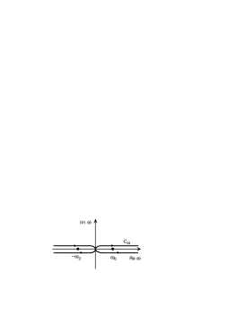
Figure 1: The integration contour for spectral integral in complex $\omega$-plane.

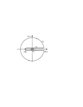
Figure 2: The integration contours for spectral integral in the complex $z$-plane.

The sum rule can also be computed by integrating along a circle ${\cal C}_{R}$ at $R\!\rightarrow\!\infty$, shown also in figure 2. We now assume that this is true in general for the full physical propagator $G$. This means that $G$ must have a residue equal to unity at $|z|\!=\!\infty$, which is equivalent to the following simple boundary condition

$$\mbox{$$}G\rightarrow\frac{1}{z}\,,\qquad{\rm when}\;|z|\rightarrow\infty.$$ (9)

More generally we will assume that any spectral integral of the form $\int d\omega\omega{\cal A}{\cal T}$, where ${\cal T}$ is some dynamical quantity, is to be computed by a contour integral of $G{\cal T}$ over a contour ${\cal C}$ which contains contributions from all poles and possible discontinuities of the propagator.

As was already pointed out, the first nontrivial correction to the propagator equation (5) occurs at the second order in gradients. To this order one finds the following equation for the complex valued $G$:

$$\mbox{$$}(k^{2}-m^{2})G+\frac{1}{4}\left(\partial_{x}^{2}+\frac{1}{2}m^{2\,\prime\prime}\partial_{k_{x}}^{2}\right)G=1,$$ (10)

where for simplicity we considered a stationary case $m^{2}=m^{2}(x)$, again with $x^{\mu}=(0,x,0,0)$. Assuming that the derivative corrections are small, it is appropriate to use an iterative procedure, which to the lowest nontrivial order gives

$$\mbox{$$}G_{2}=\frac{1}{z}-\frac{\delta_{2}}{z^{3}}-\frac{\delta_{1}}{z^{4}}$$ (11)

where $\delta_{2}=m^{2\,\prime\prime}/2$, and $\delta_{1}=(m^{2\,\prime})^{2}/2+k_{z}^{2}m^{2\,\prime\prime}$. A similar iterative procedure was used in Eq. (4), when constructing the WKB approximation to the wave function. In the rest of this letter we explain in what sense this iterative procedure can be interpreted as the semiclassical approximation to the propagator.

Let us mention that the multiple pole form of the propagator (11) can, in a loose sense, be reconciled with the picture of quasiparticle excitations. To see this, note that to the second order in gradients $G_{2}$ can equivalently be written as

$$\mbox{$$}G_{2}^{\prime}=\frac{z^{2}}{z^{3}+\delta_{2}z+\delta_{1}}\equiv\sum_{n=0}^{2}\frac{a_{n}}{z-z_{n}}\,,$$ (12)

where $a_{n}$ denote the residues at the simple poles $z_{n}$. These residues and poles are in general complex however, yielding unphysical complex dispersion relations $z=z_{n}$ and weights $a_{n}$. Indeed, the true physical meaning of the semiclassical propagator emerges only when $G$ is understood in an operational sense inside the spectral integral over the complex path in the sense conjectured above.

3 Recovering the WKB result

To study the physical consequences of Eq. (5) in more detail, without overly complicating the calculations, we now make the same simplifying assumption that was used to obtain the equation (2): $\partial_{x}^{n}m^{2}=0$ for $n\geq 2$. Without further approximations Eq. (5) then becomes

$$\mbox{$$}\delta^{3}\frac{d^{2}G}{dz^{2}}+zG=1\,,$$ (13)

where $\delta_{1}/2\rightarrow\delta^{3}=(m^{2\,\prime})^{2}/4$ and $z=k^{2}-m^{2}$. The standard solution of (13) is known. The associated Airy function $\rm Hi(z)$ [10] is unphysical however, because it does not satisfy the boundary condition (9) and it has no isolated poles, making it impossible to satisfy the sum rule. However, we can obtain a formal series solution with the desired properties through an iterative procedure:

$$\mbox{$$}G=\lim_{N\rightarrow\infty}\frac{1}{z}\sum_{n=0}^{N}(-1)^{n}\frac{(3n)!}{3^{n}n!}\left(\frac{\delta}{z}\right)^{3n}\,.$$ (14)

This can further be formally resummed to yield

$$\mbox{$$}G=\lim_{\Lambda\rightarrow\infty}\frac{1}{z}\int_{0}^{\Lambda}due^{-u-\frac{1}{3}(u\delta/z)^{3}}\,.$$ (15)

In the limit $\Lambda\rightarrow\infty$, $G$ is in fact equivalent to the associated Airy function for positive real $z$, but it diverges for ${\rm Re\,}[z^{3}]<0$. This divergent behaviour is to be expected due to the unbounded nature of Eq. (13), and it is also present in the series solution, which is formally divergent for any finite $|z|$. However, we show below that taking a finite $\Lambda$ in (15), or truncating the asymptotic series in Eq. (14) to some finite $N$, leads to a meaningful regularization, and in fact to the best estimator for the propagator.

To this end consider spectral integrals of the form

$$\mbox{$$}G[{\cal T}]\equiv\frac{2}{\pi}\int_{0}^{\infty}dk_{x}{\cal A}{\cal T}\rightarrow\frac{i}{2\pi}\oint_{{\cal C}_{z}}\frac{dz}{\sqrt{k_{0}^{2}-z}}G{\cal T},$$ (16)

where $z=k_{0}^{2}-k_{x}^{2}$ with $k_{0}^{2}=\omega^{2}-\vec{k}_{\scriptscriptstyle\parallel}^{\,2}-m^{2}$, and the contour ${\cal C}_{z}$ is the one shown in figure 2. The test function $\cal T$ representing a dynamical quantity can be any meromorphic function with no poles on the real $\omega$-axis. Note that, as a consequence of separability of spectral and dynamical properties, this is true for the important example of the generalized distribution function in the dynamical Schwinger-Dyson equation. Furthermore, ${\cal T}$ must admit a Taylor expansion around the propagator poles, i.e. it admits gradient expansion.

We chose integration over momenta rather than frequencies in Eq. (16) to facilitate direct comparison with the standard form of the semiclassical result in Eq. (4). Expanding ${\cal T}$ into the Taylor series in $k$ around $k=k_{0}$, and computing the residue one obtains

$$\mbox{$$}G[{\cal T}]={\rm Res}\left[G{\cal T}/\sqrt{k_{0}^{2}-z}\,\right]_{z=0}=\sum_{n=0}^{\infty}t_{n}{\cal T}^{(n)}_{0}\,$$ (17)

where ${\cal T}_{0}\equiv{\cal T}(k_{0})$, ${\cal T}_{0}^{\prime}\equiv(\partial_{k_{x}}{\cal T})_{k_{x}=k_{0}}$, etc. It suffices to consider the first two terms in (17) to obtain the semiclassical dispersion relation. Indeed,

$$\mbox{$$}G[{\cal T}] = \frac{{\cal T}_{0}}{k_{\rm sc}}+\left(1-\frac{k_{0}}{k_{\rm sc}}\right){\cal T}_{0}^{\prime}+{\cal O}(\cal T^{\prime\prime})$$ (18)

$$= \frac{{\cal T}(k_{\rm sc})}{k_{\rm sc}}+{\cal O}(\cal T^{\prime\prime})\,,$$

where

$$\mbox{$$}\frac{k_{0}}{k_{\rm sc}}=\frac{1}{\sqrt{\pi}}\sum_{n=0}^{\infty}(-1)^{n}\frac{\Gamma(3n+1/2)}{3^{n}n!}\left(\frac{\delta}{k_{0}^{2}}\right)^{3n}.$$ (19)

It can now be easily verified by inspection, that $k_{\rm sc}$ is equivalent to the WKB momentum $k_{x}$ in Eq. (4). Moreover, one finds that under the assumption $\partial_{x}^{n}m^{2}=0$ for $n\geq 2$, Eq. (3) reduces to the following differential equation: $y^{\prime\prime\prime}+\zeta y^{\prime}+y/2=0$ for $y=\delta^{1/2}/k_{\rm sc}$, where $\zeta\equiv k_{0}^{2}/\delta$ and $y^{\prime}\equiv dy/d\zeta$, also satisfied by the solution (19).

In figure 3 we plot the relative deviation $\kappa=k_{\rm sc}/k_{0}-1$ from the unperturbed momentum $k_{0}$ vs. $\delta/k_{0}^{2}$ for the three lowest order solutions (2nd, 4th and 6th order in gradients) as well as the formally resummed integral representation

$$\mbox{$$}\frac{k_{0}}{k_{\rm sc}}=\int_{0}^{\infty}\frac{du}{\sqrt{\pi u}}\;e^{-u-\frac{1}{3}(u\delta/k_{0}^{2})^{3}}\,.$$ (20)

For small $\delta/k_{0}^{2}$ the agreement is extremely good and it becomes progressively worse as $\delta/k_{0}^{2}$ approaches 0.3. It can be shown that the highest possible accuracy of the order $\exp-(2/3)(k_{0}^{2}/\delta)^{3/2}$ is reached by the propagator $G_{2N}$ truncated at the $2N$-th order in derivatives, where $N$ is defined by $\delta\approx\Delta_{2N}=k_{0}^{2}(1/3N)^{2/3}$. In fact the integral expression is just the envelope of $G_{2N}$’s at $\delta\approx\Delta_{2N}$, and hence represents the best possible estimate of $k_{\rm sc}$ for any value $\delta\leq\Delta_{2}$. However, even though the integral gives a reasonable result also for large values $\delta>\Delta_{2}$, one should be careful in attributing a physical meaning to it, because analytic continuation of an asymptotic series is not unique.

It is interesting to note that in the case of the electroweak phase transition the expanding phase transition front typically has a width $\sim 10-20/T$[3], so that typically $\delta/k_{0}^{2}\mbox{\raisebox{-2.58334pt}{~{}$\stackrel{{\scriptstyle<}}{{\sim}}$~{}}}0.1$. In this region the asymptotic series is accurate to 10 decimal points.

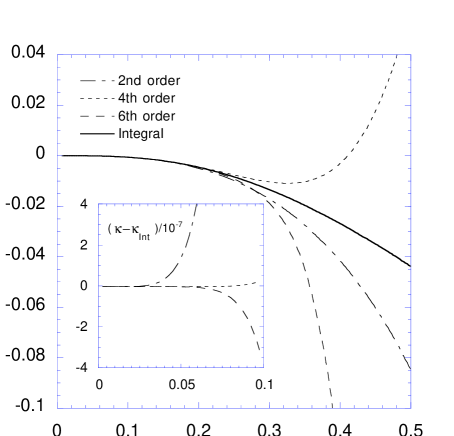
Figure 3: Plotted is the quantity $\kappa\equiv k_{\rm sc}/k_{0}-1$ for three lowest order gradient approximations for $G$ along with the formal integral solution (solid line). Inset: deviation of $\kappa_{n}$ from the integral result for small $\delta/k_{0}^{2}$.

We have seen that the semiclassical spectral function projects a dynamical quantity $\cal T$ “on-shell” by shifting the energy hypersurface from $k_{0}$ to $k_{\rm sc}\!=\!k_{\rm sc}(\omega,\vec{k}_{\scriptscriptstyle\parallel};x)$. This projection however induces additional structure in Eq. (17) contained in the higher order derivative terms ${\cal T}^{\prime\prime}_{0}$, etc., and hence the semiclassical limit in field theory cannot be described by a single on-shell function and the semiclassical dispersion relation. This is a direct consequence of the higher order poles in the semiclassical propagator, which occur generically in the presence of a space-time varying background. Note that only a finite number of terms in the expansion in ${\cal T}^{(n)}_{0}$ in Eq. (16) contribute. Indeed, the coefficient of the $n$-th order derivative ${\cal T}^{(n)}_{0}/n!$ has the form $(\sqrt{k_{0}^{2}-z}-k_{0})^{n}\!=\!(-1)^{n}(z/2k_{0})^{n}\!+\!{\cal O}(z^{n+1})$, and hence the asymptotic series representation (14) of $G$ implies that, at the order $2N$ in gradients, only the elements ${\cal T}^{(n)}_{0}$ with $n\leq 3N$ can have nonvanishing coefficients. For example, using the second order approximation to the propagator in Eqs. (11–12), the series in Eq. (17) has only 4 terms, terminating with $(\delta^{3}/24k_{0}^{4}){\cal T}_{0}^{\prime\prime\prime}$. The meaning of these corrections can be fully appreciated only when studying the semiclassical approximation of concrete dynamical quantities. Of particular importance is the quantum Boltzmann equation, which can be obtained from the dynamical Schwinger-Dyson equation by the method of spectral projection described in this letter. In this case the test function is related to the density matrix of the system and so the higher order derivative terms represent nonvanishing off-diagonal correlations between different momentum states. This is just a reflection of the uncertainty principle, according to which localisation in the position necessarily implies delocalization in the momentum.

4 Conclusions

In this letter we studied the semiclassical limit in field theory. We found that in the presence of slowly varying backgrounds, there is a simple iterative procedure by which one can construct the semiclassical propagator as a semi-convergent asymptotic series controlled by powers of gradients. While we discussed at length the simple case $\partial_{x}^{n}m^{2}=0$ for $n\geq 2$, the method can straightforwardly be extended to the general case with higher derivatives and nonvanishing self-energy. The semiclassical dispersion relation appears in a nontrivial way through study of spectral integrals and cannot be associated to a simple shift of the pole of the propagator. We further found that the spectral projection of a dynamical quantity necessarily contains higher order momentum derivatives as a reflection of localization in coordinate space. As a consequence the plasma dynamics is not described by a single classical Boltzmann equation, but instead by a set of independent equations describing not only evolution of the distribution function, but also of a limited number of its derivatives. We will pursue this issue in a forthcoming publication.

References

- [1]
- [2] G. Wentzel, Z. Physik 38, 518 (1926); K.A. Kramers Z. Physik 39, 828 (1926); L. Brillouin, Compt. Rend. 183, 24 (1926).
- [3] For review see for example V. Rubakov and M.E. Shaposhnikov, Phys. Usp. 39, 461 (1996).
- [4] G. Moore and T. Prokopec, Phys. Rev. D52, 7182 (1995).
- [5] J.M. Cline and G. Moore, Phys. Rev. Lett. 81, 3315 (1998).
- [6] M. Joyce, T. Prokopec and N. Turok, Phys. Rev. D53, 2958 (1996).
- [7] J.M. Cline, M. Joyce and K. Kainulainen, Phys. Lett. B417, 79 (1998); Erratum, ibid. B448, 321 (1999).
- [8] L.P. Kadanoff and G. Baym, Quantum Statistical Mechanics, Benjamin Press, New York (1962); P. Danielewicz, Ann. Phys. 152, 239 (1984); J. Rammer and H. Smith, Rev. Mod. Phys. 58, 323 (1986).
- [9] P. Henning, Phys. Rep. 253, 235 (1995).
- [10] M. Abramowiz and I.A. Stegun, Handbook of mathematical functions, Dover Publications Inc., New York (1972).