Abstract

We present a general method for extracting the Gell Mann-Low logarithmic derivative of an effective charge of an observable directly from data as a mean for empirically verifying the universal terms of the QCD $\beta$-function. Our method avoids the biases implicit in fitting to QCD-motivated forms as well as the interpolation errors introduced by constructing derivatives from discrete data. We also derive relations between moments of effective charges as new tests of perturbative QCD.

Submitted to Physical Review D

1 Introduction

An effective charge [2] encodes the entire perturbative correction of a QCD observable; for example, the ratio of $e^{+}e^{-}\gamma^{*}\to{\rm hadrons}$ annihilation to muon pair cross sections can be written

$$R_{e^{+}e^{-}}(s)\equiv\frac{\sigma(e^{+}e^{-}\rightarrow{\rm hadrons})}{\sigma(e^{+}e^{-}\rightarrow\mu^{+}\mu^{-})}=R_{e^{+}e^{-}}^{0}(s)\left(1+\frac{\alpha_{R}(\sqrt{s})}{\pi}\right),$$ (1)

where $R^{0}_{e^{+}e^{-}}$ is the prediction at Born level. More generally, the effective charge $\alpha_{A}(Q)$ is defined as the entire QCD radiative contribution to an observable ${\cal O}_{A}(Q)$ [2]:

$${\cal O}_{A}(\Lambda)={\cal O}_{A}^{0}\left(\delta_{A}+\frac{\alpha_{A}(\Lambda)}{\pi}\right),$$ (2)

where $\delta_{A}$ is the zeroth order QCD prediction (i.e., the parton model), and $\alpha_{A}(\Lambda)/\pi$ is the entire QCD correction. Note that $\delta_{A}=0$ or $1$ depending on whether the observable A exists at zeroth order. Important examples with $\delta_{A}=1$ are the $e^{+}e^{-}$ annihilation cross-section ratio and the $\tau$ lepton’s hadronic decay ratio,

$$R_{\tau}\equiv\frac{\Gamma(\tau^{-}\rightarrow{\nu_{\tau}+{\rm hadrons}})}{\Gamma(\tau^{-}\rightarrow{\nu_{\tau}e^{-}\bar{\nu_{e}}})}=R_{\tau}^{0}\left(1+\frac{\alpha_{\tau}(m_{\tau})}{\pi}\right).$$ (3)

In contrast, the effective charge $\alpha_{V}(Q)$ defined from the static heavy quark potential and the effective charge $\alpha_{>2\,\hbox{jets}}$ defined from $e^{+}e^{-}$ annihilation into more than two jets, $\sigma_{>2\,\hbox{jets}}$, have $\delta_{A}=0$.

One can define effective charges for virtually any quantity calculable in perturbative QCD; e.g., moments of structure functions, ratios of form factors, jet observables, and the effective potential between massive quarks. In the case of decay constants of the $Z$ or the $\tau$, the mass of the decaying system serves as the physical scale in the effective charge. In the case of multi-scale observables, such as the two-jet fraction in $e^{+}e^{-}$ annihilation, the arguments of the effective coupling $\alpha_{2jet}(s,y)$ correspond to the overall available energy and characteristic kinematical jet mass fraction. Effective charges are defined in terms of observables and, as such, are renormalization-scheme and renormalization-scale independent.

The scale $Q$ which enters a given effective charge corresponds to its physical momentum scale. The total derivative of each effective charge $\alpha_{A}(Q)$ with respect to the logarithm of its physical scale is given by the Gell Mann-Low function:

$$\Psi_{A}[\alpha_{A}(Q,m),Q/m]\equiv{d\alpha_{A}(Q,m)\over d\log Q},$$ (4)

where the functional dependence of $\Psi_{A}$ is specific to the effective charge $\alpha_{A}$. Here $m$ refers to the quark’s pole mass. The pole mass is universal in that it does not depend on the choice of effective charge. It should be emphasized that the Gell Mann-Low $\Psi$ function is a property of a physical quantity, and it is thus independent of conventions such as the renormalization procedure and the choice of renormalization scale.

A central feature of quantum chromodynamics is asymptotic freedom; i.e., the monotonic decrease of the QCD coupling $\alpha_{A}(Q^{2})$ at large spacelike scales. The empirical test of asymptotic freedom is the verification of the negative sign of the Gell Mann-Low function at large momentum transfer, a feature which must in fact be true for any effective charge.

In perturbation theory,

$$\Psi_{A}=-\Psi_{A}^{\{0\}}{\alpha_{A}^{2}\over\pi}-\Psi_{A}^{\{1\}}{\alpha_{A}^{3}\over\pi^{2}}-\Psi_{A}^{\{2\}}{\alpha_{A}^{4}\over\pi^{3}}+\cdots$$ (5)

At large scales $Q^{2}>>m^{2}$, where the quarks can be treated as massless, the first two terms are universal [3] and basically given by the first two terms of the usual QCD $\beta$ function for $N_{C}=3$

$$\Psi_{A}^{\{0\}} = \frac{\beta_{0}}{2}=\frac{11}{2}\,-\frac{1}{3}\,N_{F,A}^{\{0\}},$$

$$\Psi_{A}^{\{1\}} = \frac{\beta_{1}}{8}=\frac{51}{4}\,+\frac{19}{12}\,N_{F,A}^{\{1\}}.$$ (6)

Unlike the $\beta$-function which controls the renormalization scale dependence of bare couplings such as $\alpha_{\overline{M}S}(\mu)$, the $\psi$ function is analytic in $Q^{2}/m^{2}$. In the case of the $\alpha_{V}$ scheme, the effective charge defined from the heavy quark potential, the functional dependence of $N_{F,V}(Q^{2}/m^{2})$ is known to two loops [5].

The purpose of this paper is to develop an accurate method for extracting the Gell Mann-Low function from measurements of an effective charge in a manner which avoids the biases and uncertainties present either in a standard fit or in numerical differentiation of the data. We will show that one can indeed obtain strong constraints on $\Psi_{A}^{\{0\}}$ and $\Psi_{A}^{\{1\}}$ from generalized moments of the measured quantities which define the effective charge. We find that the weight function $f(\xi)$ which defines the effective charge $\alpha_{Af}(\Lambda)$ from an integral of the effective charge $\alpha_{A}(Q)$ can be chosen to produce maximum sensitivity to the Gell-Mann Low function. As an example we will apply the method to the $e^{+}e^{-}$ annihilation into more than two jets. Clearly one could also extract the Gell Mann-Low function directly from a fit to the data, but the fact that we are dealing with a logarithmic derivative introduces large uncertainties [4]. Our results minimize some of these uncertainties. In addition, our analysis provides a new class of commensurate relations between observables which are devoid of renormalization scheme and scale artifacts.

One can define generalized effective charges from moments of the observables. The classic example is $\alpha_{\tau}(\Lambda)$ where $\Lambda$ is the generalization of the lepton mass. The relevant point is that $R_{\tau}$ can be written as an integral of $R_{e^{+}e^{-}}$ [6], as follows:

$$R_{\tau}(\Lambda^{2})=\frac{2}{\sum_{f}q_{f}^{2}}\int_{0}^{\Lambda^{2}}\,\frac{ds}{\Lambda^{2}}\left(1-\frac{s}{\Lambda^{2}}\right)^{2}\left(1+\frac{2s}{\Lambda^{2}}\right)R_{e^{+}e^{-}}(s),$$ (7)

where $q_{f}$ are the quark charges. As a consequence of the mean value theorem, the associated effective charges are related by a scale shift

$$\alpha_{\tau}(\Lambda)=\alpha_{R}(\sqrt{s}=\Lambda_{\tau}),$$ (8)

The ratio of scales $\Lambda_{\tau}/\Lambda$ in principle is predicted by QCD [7]: The prediction at NLO is [7]

$${\Lambda_{\tau}\over\Lambda}=\exp\left[-{19\over 24}-{169\over 128}{\alpha_{R}(\Lambda_{\tau})\over\pi}+\cdots\right].$$ (9)

Such relations between observables are called commensurate scale relations (CSR) [7].

The relation between $R_{\tau}$ and $R_{e^{+}e^{-}}$ suggests that we can obtain additional useful effective charges by changing the functional weight appearing in the integrand. Indeed it has been shown [8] that, starting from any given observable ${\cal O}_{A}$ we can obtain new effective charges $\alpha_{A\,f}$ by constructing the following quantity

$${\cal O}_{A\,f}(\Lambda)=C\int_{\Lambda^{2}_{1}(\Lambda)}^{\Lambda^{2}_{2}(\Lambda)}\,\frac{ds}{\Lambda^{2}}f\left(\frac{\sqrt{s}}{\Lambda}\right){\cal O}_{A}(\sqrt{s}),$$ (10)

where $C$ is a constant and $f(\xi)$ is a positive arbitrary integrable function. In order for ${\cal O}_{A\,f}$ to define an effective charge $\alpha_{A\,f}$ through

$${\cal O}_{A\,f}(\Lambda)={\cal O}^{0}_{A\,f}\left(\delta_{A}+\frac{\alpha_{A\,f}(\Lambda)}{\pi}\right),$$ (11)

it is necessary that $\Lambda_{1}(\Lambda)=\lambda_{1}\Lambda$ and $\Lambda_{2}(\Lambda)=\lambda_{2}\Lambda$, with both $\lambda_{1}$ and $\lambda_{2}$ constant. Then, by the mean value theorem, $\alpha_{A\,f}$ is related again to $\alpha_{A}$ by a scale shift

$$\alpha_{A\,f}(\Lambda)=\alpha_{A}(\Lambda_{Af}),$$ (12)

with $\Lambda_{1}<\Lambda_{Af}<\Lambda_{2}$. An important observation [8] is that PQCD predicts $\lambda_{Af}=\Lambda_{Af}/\Lambda$ to leading twist. If we ignore quark masses so that the two first coefficients of the Gell-Mann Low function are constant, one has

$$\frac{\alpha_{A}(\sqrt{s})}{\pi}=\frac{\alpha_{A}(\Lambda)}{\pi}-\frac{\Psi_{0}}{2}\ln{\left(\frac{s}{\Lambda^{2}}\right)}\left(\frac{\alpha_{A}(\Lambda)}{\pi}\right)^{2}+$$ (13)

$$\quad+\frac{1}{4}\left[\Psi_{0}^{2}\ln^{2}\left(\frac{s}{\Lambda^{2}}\right)-2\,\Psi_{1}\ln\left(\frac{s}{\Lambda^{2}}\right)\right]\left(\frac{\alpha_{A}(\Lambda)}{\pi}\right)^{3}\ldots$$

If we now use eqs.(10) and (11), we find [8]

$$\frac{\alpha_{Af}(\Lambda)}{\pi} = \frac{\alpha_{A}(\Lambda)}{\pi}-\frac{\Psi_{0}}{2}\frac{I_{1f}}{I_{0f}}\left(\frac{\alpha_{A}(\Lambda)}{\pi}\right)^{2}$$ (14)

$$+ \frac{1}{4}\left[\Psi_{0}^{2}\frac{I_{2f}}{I_{0f}}-2\,\Psi_{1}\frac{I_{1f}}{I_{0f}}\right]\left(\frac{\alpha_{A}(\Lambda)}{\pi}\right)^{3}\ldots,$$

where $I_{lf}=\int^{\lambda^{2}_{2}}_{\lambda^{2}_{1}}f(\xi)(\ln{\xi^{2}})^{l}d\,\xi^{2}$ is independent of the choices of observable $A$ and scale $\Lambda$, but only provided that $\Lambda_{1}(\Lambda)=\lambda_{1}\Lambda$ and $\Lambda_{2}(\Lambda)=\lambda_{2}\Lambda$. Replacing $s$ by $\Lambda^{2}_{A\,f}$ in eq. (13) and comparing with eq. (14), we find

$$\lambda_{Af}=\exp\left\{\frac{I_{1f}}{2I_{0f}}+\frac{\Psi_{0}}{4}\left[\left(\frac{I_{1f}}{I_{0f}}\right)^{2}-\frac{I_{2f}}{I_{0f}}\right]\frac{\alpha_{A}(\Lambda)}{\pi}\;...\right\}.$$ (15)

In general the commensurate scale relation will have the following expansion

$$\ln\lambda_{Af}(\Lambda)=\sum_{n=0}^{\infty}a_{f}^{(n)}\left(\frac{\alpha_{A}(\Lambda)}{\pi}\right)^{n},$$ (16)

where the first three coefficients are independent of $A$. Note that the above formulae are only valid inside regions of constant $N_{F}$ and sufficiently apart from quark thresholds. If we include the mass dependence, the effective charges, by the mean value theorem, are still related by a scale shift, although it cannot be written in the simple form of eq. (15). Indeed, even the lowest order of $\lambda_{A\,f}$ would have a small dependence on the energy and the effective number of flavors appearing in $\Psi_{0}$.

2 Obtaining the Gell Mann-Low function directly from observables

The main practical obstacle in determining the Gell Mann-Low function from experiment is that it is a logarithmic derivative. One can try to obtain the value of the parameters of the $\Psi$ function from a direct fit to the data using the QCD forms, but any approximation to the derivative of the experimental results implicitly requires extrapolation or interpolation of the data. In order to observe a significant variation of the effective charge $\alpha_{A}$ one needs to compare two vastly separated scales. This is illustrated in Fig.1. However, to approximate $\Psi(\sqrt{s})\simeq\Delta\alpha_{A}(\sqrt{s})/(\Delta\ln\sqrt{s})$ with a huge separation between $\sqrt{s}$ and $\sqrt{s^{\prime}}$ is not very accurate since then the value for $\Delta\alpha_{A}/\Delta\ln\sqrt{s}$ is the slope of the $Q$ straight line in Fig. 1 instead of that of $P$, which gives an ${\cal O}(\Delta\ln\sqrt{s})^{2}$ error. If we want to obtain $\Psi$ from a finite difference approximation, we need to interpolate $\Delta\ln\sqrt{s}\rightarrow 0$, but in this case the experimental errors will most likely be much larger than the required precision. Such an interpolation procedure has already been applied in ref. [4] near the $\tau$ region to test the running of $\alpha_{s}$ (including appropriate corrections to the leading twist formalism). In this energy region the value of the QCD coupling is rather large, and the interpolation yields evidence for some running. However, it has also been pointed out in [4], that the value of the coupling extrapolated from the $\tau$ region to high energies appears small compared to direct determinations.

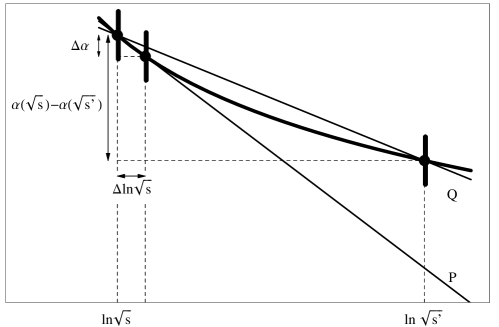
Figure 1: Finite difference approximation of $\Psi$. If one takes $\Delta\ln\sqrt{s}$ very small, the errors can be larger than $\Delta\alpha$, and the result will be meaningless. This can be avoided by choosing very far separated points $\sqrt{s}$ and $\sqrt{s^{\prime}}$, but then the approximation yields the slope of line $Q$ instead of that of $P$.

In the next section we shall use the effective charge formalism to derive several expressions within leading twist QCD which relate the intrinsic $\Psi_{A}$ function of $\alpha_{A}$ directly to the observables ${\cal O}_{A}$. We shall show that with just three data points we can obtain good sensitivity to the value of $\Psi_{0}$ without any numerical differentiation or fit.

2.0.1 Differential Commensurate Scale Relations

Let us formally differentiate eq. (10) with respect to $\Lambda$

$$\frac{d{\cal O}_{A\,f}(\Lambda)}{d\Lambda} = \frac{2\,C}{\Lambda}\left[\lambda_{2}^{2}f(\lambda_{2})\,{\cal O}_{A}(\Lambda_{2})-\lambda_{1}^{2}f(\lambda_{1})\,{\cal O}_{A}(\Lambda_{1})\right]$$ (17)

$$- \frac{2{\cal O}_{A\,f}(\Lambda)}{\Lambda}-\frac{C}{\Lambda}\int_{(\lambda_{1}\Lambda)^{2}}^{(\lambda_{2}\Lambda)^{2}}\frac{ds}{\Lambda^{2}}\,{\cal O}_{A}(\sqrt{s})\frac{\sqrt{s}}{\Lambda}\frac{df(\sqrt{s}/\Lambda)}{d(\sqrt{s}/\Lambda)}.$$

The first term in the right-hand side can be obtained directly from the data on ${\cal O}_{A}$. This is also the case for the second term, after using eqs. (2) and (12), since

$${\cal O}_{A\,f}(\Lambda)={\cal O}_{A\,f}^{0}\left(\delta_{A}+\frac{\alpha_{A\,f}(\Lambda)}{\pi}\right)={\cal O}_{A\,f}^{0}\left(\delta_{A}+\frac{\alpha_{A}(\Lambda_{f})}{\pi}\right)=\frac{{\cal O}_{A\,f}^{0}}{{\cal O}_{A}^{0}}\,{\cal O}_{A}(\Lambda_{f}),$$ (18)

Note that ${\cal O}_{A\,f}^{0}$ and ${\cal O}_{A}^{0}$ are known constants. Finally, there is a choice of $f(\xi)$ which allows us to recast the third term in the right-hand side of eq. (17) and provide a direct relation between the data and the effective charge. Namely, we choose

$$\xi\,\frac{df(\xi)}{d\xi}=\rho\,f(\xi),$$ (19)

with $\rho$ any real number. That is, up to an irrelevant multiplicative constant, we take

$$f(\xi)=\xi^{\rho}.$$ (20)

With this choice eq. (17) can be simply written as

$$\frac{d{\cal O}_{A\,\rho}(\Lambda)}{d\Lambda}=\frac{2C}{\Lambda}\left[\lambda_{2}^{\rho+2}{\cal O}_{A}(\Lambda_{2})-\lambda_{1}^{\rho+2}{\cal O}_{A}(\Lambda_{1})\right]-\frac{\rho+2}{\Lambda}{\cal O}_{A\,\rho}(\Lambda).$$ (21)

Note that, to simplify the notation, we have substituted the $f$ subscript by $\rho$. In terms of $\Psi_{A}$ this means

$$\Psi_{A\,\rho}(\Lambda)=\Lambda\,\frac{d\alpha_{A\,\rho}(\Lambda)}{d\Lambda}=\frac{\pi\Lambda}{{\cal O}_{A\,\rho}}\,\frac{d{\cal O}_{A\,\rho}(\Lambda)}{d\Lambda}.$$ (22)

But using its definition, we can easily see that

$${\cal O}_{A\,\rho}^{0}=\frac{2\,C\,{\cal O}_{A}^{0}}{(\rho+2)}(\lambda_{2}^{\rho+2}-\lambda_{1}^{\rho+2}),$$ (23)

so that, using eq. (18), we arrive at

$$\Psi_{A\,\rho}(\Lambda)=\pi\frac{\rho+2}{{\cal O}_{A}^{0}}\left[\frac{\lambda_{2}^{\rho+2}{\cal O}_{A}(\Lambda_{2})-\lambda_{1}^{\rho+2}{\cal O}_{A}(\Lambda_{1})}{\lambda_{2}^{\rho+2}-\lambda_{1}^{\rho+2}}-{\cal O}_{A}(\Lambda_{\rho})\right],$$ (24)

Note that we have just written $\Psi_{A\,\rho}(\Lambda)$ directly in terms of observables. Therefore, we have related the universal $\Psi_{0}$ and $\Psi_{1}$ coefficients directly to observables, without any dependence on the renormalization scheme or scale.

Up to this point $\Lambda_{1}$ and $\Lambda_{2}$ are arbitrary. In order to illustrate the meaning of eq.(24), we now choose $\lambda_{1}=0$ and $\lambda_{2}=1$, so that eq.(24) becomes:

$$\Psi_{A\,\rho}(\Lambda)=\pi\frac{\rho+2}{{\cal O}_{A}^{0}}\left[{\cal O}_{A}(\Lambda)-{\cal O}_{A}(\Lambda_{\rho})\right],$$ (25)

Let us remark that, although it may look similar, the above equation is not the finite difference approximation

$$\Psi_{A}(\Lambda)\simeq\frac{\pi\,\Lambda}{{\cal O}^{0}_{A}}\,\frac{{\cal O}_{A}(\Lambda)-{\cal O}_{A}(\Lambda-\Delta\Lambda)}{\Delta\Lambda}+O(\Delta\Lambda^{2})$$ (26)

which is a good numerical approximation to $\Psi_{A}(\Lambda)$ when $\Delta\Lambda$ is very small. In contrast, eq. (24), is exact (at leading twist) no matter whether $\Lambda-\Lambda_{\rho}$ is big or small.

However, we do not want to set $\lambda_{1}=0$, since then the integrated effective charges defined in eq.(10), contain higher twist contributions which are unsuppressed at low energies, and our leading twist formulae would be invalid in practice. In addition, some observables like the number of jets produced in $e^{+}e^{-}$ annihilation are only well defined above some energy, which becomes a lower cutoff in the integral of eq.(10).

Nevertheless, by choosing $\Lambda$ and $\lambda_{2}$ appropriately, we can obtain any value of $\Lambda_{1}\neq 0$ and $\Lambda_{2}\neq 0$, even if we set $\lambda_{1}=1$, and so we will do so in the following. That is:

$$\Psi_{A\,\rho}(\Lambda)=\pi\frac{\rho+2}{{\cal O}_{A}^{0}}\left[\frac{\lambda_{2}^{\rho+2}{\cal O}_{A}(\Lambda_{2})-{\cal O}_{A}(\Lambda)}{\lambda_{2}^{\rho+2}-1}-{\cal O}_{A}(\Lambda_{\rho})\right],$$ (27)

which is an exact formula relating $\Psi_{A}$ with the observable ${\cal O}_{A}$ at three scales $\Lambda<\Lambda_{\rho}<\Lambda_{2}$.

It happens, however, that we are interested in measuring not the $\Psi_{A\,\rho}$ intrinsic function but $\Psi_{A}$ itself. We thus arrive at our final result:

$$\Psi_{A}(\Lambda\,\lambda_{\rho}(\Lambda))\left[1+\frac{\lambda^{\prime}_{\rho}}{\lambda_{\rho}}\right]=\pi\,\frac{\rho+2}{{\cal O}_{A}^{0}}\left[\frac{\lambda_{2}^{\rho+2}{\cal O}_{A}(\Lambda_{2})-{\cal O}_{A}(\Lambda)}{\lambda_{2}^{\rho+2}-1}-{\cal O}_{A}(\Lambda\lambda_{\rho})\right].$$ (28)

where we have also defined $\lambda_{\rho}=\Lambda_{\rho}/\Lambda$. Note that $\Psi_{A}$ appears in the above equation both at $\Lambda_{\rho}$ and $\Lambda$ through the $\lambda^{\prime}_{\rho}$ coefficient, defined as $d\lambda/dLog\Lambda$, which only vanishes at leading order. Therefore, if we include higher order contributions the above equation is not enough to determine $\Psi_{A}$ at one given scale.

Let us work out first the implications of eq.(28) at leading order, since it contains all the relevant features of our approach.

2.1 Leading order

Suppose then that we had three experimental data points at $s_{a}<s_{b}<s_{c}$. In order to apply eq. (27), we first identify $\Lambda_{2}=\sqrt{s_{c}/s_{a}}$ and then we obtain the $\rho$ such that $\sqrt{s_{a}}=\sqrt{s_{b}}/\lambda_{\rho}$.

The $I_{k\rho}$ integrals are given by

$$I_{k\rho}=\frac{k!}{\rho/2+1}\sum_{j=1}^{2}\left[(-1)^{j}\,\lambda_{2}^{\rho+2}\sum_{l=0}^{k}\left(\frac{(\ln\lambda_{2}^{2})^{(k-l)}(-1)^{l}}{(\rho/2+1)^{l}(k-l)!}\right)-\frac{(-1)^{k}}{(\rho/2+1)^{k}}\right].$$ (29)

Thus, at leading order we have to obtain $\rho$ from

$$\ln\frac{s_{b}}{s_{a}}=2\ln\lambda_{\rho}=\frac{I_{1\rho}}{I_{0\rho}}=\frac{s_{c}^{\rho/2+1}\ln(s_{c}/s_{a})}{s_{c}^{\rho/2+1}-s_{a}^{\rho/2+1}}-\frac{1}{\rho/2+1},$$ (30)

which can be evaluated numerically.

As we have already commented, at leading order $\lambda^{\prime}=0$, and therefore

$$\Psi_{A}(\sqrt{s_{b}})=\pi\,\frac{\rho+2}{{\cal O}_{A}^{0}}\left[\frac{s_{c}^{\rho/2+1}{\cal O}_{A}(\sqrt{s_{c}})-s_{a}^{\rho/2+1}{\cal O}_{A}(\sqrt{s_{a}})}{s_{c}^{\rho/2+1}-s_{a}^{\rho/2+1}}-{\cal O}_{A}(\sqrt{s_{b}})\right].$$ (31)

Let us remark once more that these are leading-twist formulae, and $s_{a},s_{b},s_{c}$ should lie in a range where higher twist effects are negligible.

2.2 Beyond leading order

As we have already seen, if we go beyond the leading order contributions, we have to use eq.(28), which does not completely determine the value of $\Psi_{A}$ at a single scale. In principle, we need an additional equation. In fact, the $\lambda^{\prime}$ term can be neglected. Intuitively, this is due to the very slow evolution of $\alpha_{A}$. Let us give some numerical values; first, we will write

$$\frac{\lambda^{\prime}_{\rho}}{\lambda_{\rho}}=\Psi_{A}(\Lambda)\Omega_{\rho}(\Lambda),$$ (32)

with

$$\Omega_{\rho}(\Lambda)\equiv\frac{d\,\ln\lambda_{\rho}}{d(\alpha_{A}(\Lambda))}=2\sum_{n=1}^{\infty}n\,a_{\rho}^{(n)}\left(\frac{{\cal O}_{A}(\Lambda)}{{\cal O}_{A}^{0}}-\delta_{A}\right)^{n-1}.$$ (33)

From PQCD we know that the expansion of $\Psi_{A}$ starts with $\alpha_{A}^{2}$. Thus, the $\lambda^{\prime}$ term in eq.(28) is an $O(\alpha_{A}^{4})$ effect. It should only be taken into account if we are interested in $\Psi$ up to that order. Numerically, the expected value of $\Psi_{A}(\Lambda)$ at the energies we will be using, ranges from $10^{-2}$ to $2\times 10^{-2}$ at most. In addition, $\Omega$ ranges from $3\times 10^{-2}$ to 0.5. Thus, even in the worst case, the $\lambda^{\prime}$ term contribution would be slightly smaller than $1\%$ of $\Psi$. If that term is to be kept, then we need and additional equation involving a fourth data point. We have found that the final error estimate increases since it is much harder to accommodate four points sufficiently separated within a given energy range. It seems that $1\%$ accuracy is the lower limit for this method. If additional higher twist corrections are included, it could be possible to extend the energy range to separate the points and improve the precision.

Therefore, in what follows we will use eq. (31). However, the NLO $\rho$ parameter is now obtained by solving numerically the equation

$$\ln\frac{s_{b}}{s_{a}} = \frac{s_{c}^{\rho/2+1}\ln^{2}(s_{b}/s_{a})}{s_{c}^{\rho/2+1}-s_{a}^{\rho/2+1}}-\frac{1}{\rho/2+1}$$

$$+ \frac{\Psi_{0}}{2}\left[\frac{(s_{a}\,s_{c})^{\rho/2+1}\ln^{2}(s_{b}/s_{a})}{(s_{c}^{\rho/2+1}-s_{a}^{\rho/2+1})^{2}}-\frac{1}{(\rho/2+1)^{2}}\right]\left(\frac{{\cal O}_{A}(\sqrt{s_{a}})}{{\cal O}^{0}_{A}}-\delta_{A}\right),$$

where $s_{a}<s_{b}<s_{c}$ and $\sqrt{s_{b}}=\lambda_{\rho}\,\sqrt{s_{a}}$ and $\sqrt{s_{c}}=\lambda_{2}\,\sqrt{s_{a}}$. Note that now $\Psi_{0}$ is an input, but the output is the NLO $\Psi$ function.

3 Error estimates

Although they have inspired our approach, observables with $\delta_{A}\neq 0$ are not well suited for our method, because the relative error in ${\cal O}_{A}(E)$ becomes at least one order of magnitude larger for the effective charge $\alpha_{A}(E)$. For example, using the $e^{+}e^{-}$ hadronic ratio defined in Sect.1, if we introduce a $1\%$ error in $R_{e^{+}e^{-}}$, the error in $\alpha_{R}$ is $O(20\%)$ and we have to separate the data points over five orders of magnitude to obtain $\Psi_{R}$ with a $10\%$ precision. In practice, that renders the method useless.

The problem we have described is avoided if we use an observable with $\delta_{A}=0$. That is the case, for instance, of the $e^{+}e^{-}$ annihilation in more than two jets, $\sigma_{>2-\hbox{jets}}(s,y)=\sigma_{\hbox{tot}}-\sigma_{2\,\hbox{jets}}$, where $y$ is used to define when two partons are unresolved [9] (i.e. their invariant mass squared is less than $ys$). This process does not occur in the parton model since it requires, at least, one gluon. Note that $\Psi_{0}$ and $\Psi_{1}$ are independent of $y$.

At LO we can work with exact results, but as soon as we introduce higher orders, there is some degree of truncation in the formulae. We have therefore first constructed simulated data following a model that corresponds to the exact LO equations. Let us remark that these are models, not QCD. They are obtained by the truncation of $\alpha_{A}$ at a given order. Thus, in principle, they will have some different features from QCD, as for instance, some residual scale dependence. In the real world this will not occur. However, we have worked out these examples for illustrative purposes to obtain a rough estimate of the errors.

3.0.1 Leading order

What we call the LO model is to use

$$\frac{\alpha_{A}(Q)}{\pi}=\frac{\alpha(M_{Z})}{\pi}-\frac{\Psi_{0}}{2}\ln\left(\frac{Q^{2}}{M_{Z}^{2}}\right)\left(\frac{\alpha_{A}(M_{Z})}{\pi}\right)^{2},$$ (35)

exactly. We have taken $\alpha_{A}(M_{Z})$ as the reference value for simplicity. Note, however, that the derivative of the above expression is

$$\Psi_{A}=-\frac{\Psi_{0}}{2}\left(\frac{\alpha_{A}(M_{Z})}{\pi}\right)^{2},$$ (36)

which is a constant which differs by $O(\alpha/\pi)^{3}$ terms from the LO PQCD result

$$\Psi_{A}(Q)=-\frac{\Psi_{0}}{2}\left(\frac{\alpha_{A}(Q)}{\pi}\right)^{2}.$$ (37)

In Table 1 we can see the estimates of the relative errors in our determination of $\Psi_{A}$, which depend on the different position of the data points, as well as in their errors $\Delta{\cal O}_{A}$. Since the observable vanishes in the parton model, the relative error in $\alpha_{A}$ is exactly that of ${\cal O}_{A}$.

$\sqrt{s_{a}}$ (GeV)	$\sqrt{s_{b}}$ (GeV)	$\sqrt{s_{c}}$ (GeV)	$\Delta{\cal O}_{A}/{\cal O}_{A}$	$\Delta\Psi_{A}/\Psi_{A}$
30	100	300	$1\,\%$	$3\,\%$
			$3\,\%$	$9.1\,\%$
400	640	1000	$1\,\%$	$6.2\,\%$
			$3\,\%$	$18.6\,\%$
500	875	1000	$1\,\%$	$4.9\%$
			$3\,\%$	$14.6\,\%$

Table 1: Estimated relative errors in the determination of $\Psi_{0}$ using the LO equations. We assume the relative error $\Delta{\cal O}_{A}/{\cal O}_{A}$ in the measurements of ${\cal O}_{A}$. The estimates correspond to an observable with a vanishing parton model contribution ($\delta_{A}=0$) such as $e^{+}e^{-}$ annihilation into more than two jets, $\sigma_{>2-\hbox{jets}}$.

The results in the table deserve some comments.

• First, the values of $\sqrt{s_{a}}$ and $\sqrt{s_{c}}$ have to be chosen to maximize their distance, within a region of constant $N_{F}$. Thinking in terms of $\sigma_{>2-\hbox{jets}}$, they correspond either to the region where both energies are sufficiently above the b-quark pair threshold but still below $t\bar{t}$ production, or both are above the $t\bar{t}$ pair threshold, in regions accessible at NLC.

• Second, we have chosen the same relative error for the measurements at the three points. The intermediate energy $\sqrt{s_{b}}$ is then tuned to minimize the error, which is obtained assuming the three ${\cal O}_{A}$ measurements are independent.

Let us remark once again that we have not used at any moment the value of $\Psi_{0}$, which is obtained from the data using this method. If we want to use higher order contributions, using the value of $\Psi_{0}$ as an input, we would obtain information about higher order coefficients, like $\Psi_{1}$ if we were to work at NLO.

3.0.2 Beyond leading order

The NLO model is now given by:

$$\frac{\alpha_{A}(Q)}{\pi} = \frac{\alpha(M_{Z})}{\pi}-\frac{\Psi_{0}}{2}\ln\left(\frac{Q^{2}}{M_{Z}^{2}}\right)\left(\frac{\alpha_{A}(M_{Z})}{\pi}\right)^{2}$$ (38)

$$+ \frac{1}{4}\left[\Psi_{0}^{2}\ln^{2}\left(\frac{Q^{2}}{\Lambda}\right)-2\,\Psi_{1}\ln\left(\frac{Q^{2}}{M_{Z}^{2}}\right)\right]\left(\frac{\alpha_{A}(M_{Z})}{\pi}\right)^{3}.$$

and therefore, we obtain

$$\Psi_{A}(Q)=-\frac{\Psi_{0}}{2}\left(\frac{\alpha_{A}(Q)}{\pi}\right)^{2}-\frac{\Psi_{1}}{2}\left(\frac{\alpha_{A}(Q)}{\pi}\right)^{3},$$ (39)

which is the QCD NLO $\Psi_{A}$ result up to $O(\alpha/\pi)^{4}$ terms. In contrast with the LO case, obtaining $\rho$ now requires some truncation of the formulae when passing from eqs. (13) and (10) to eq. (14). This is very interesting since we can thus obtain an estimate of the theoretical error due to truncation, which will be present in the real case too. It can be seen in Table 2 in the rows where $\Delta{\cal O}_{A}=0$, and it is usually $O(1\%)$.

Again we have also considered the experimental $\Delta{\cal O}_{A}(E_{i})$ uncertainties. The final error given in the last column is estimated assuming that the four experimental errors and the one due to truncation are all independent. Note that when passing from a $1\%$ experimental error to a $3\%$, the total error is not multiplied by 3, since the truncation error does not scale.

$\sqrt{s_{a}}$ (GeV)	$\sqrt{s_{b}}$ (GeV)	$\sqrt{s_{c}}$ (GeV)	$\Delta{\cal O}_{A}/{\cal O}_{A}$	$\Delta\Psi_{A}/\Psi_{A}$
			$0\%$	$2\%$
30	100	300	$1\,\%$	$2.7\,\%$
			$3\,\%$	$7.5\,\%$
			$0\%$	$.9\%$
400	640	1000	$1\,\%$	$10\,\%$
			$3\,\%$	$29\,\%$
			$0\%$	$1\%$
500	875	1000	$1\,\%$	$10\%$
			$3\,\%$	$30\,\%$

Table 2: Error estimates at NLO.

The fact that we obtain larger errors in the NLO case may seem surprising, but it is not. The reason is that the LO is a very crude approximation of the $\Psi_{A}$ QCD scaling behavior. In the LO model, the $\Psi$ function was a constant, but in the NLO it changes with the energy scale, as it occurs in the realistic case. Indeed, the evolution of $\alpha_{A}$ at high energies becomes much slower so that the difference between $\alpha_{A}$ at two given points is smaller at NLO than at LO. Hence, for the same relative errors, the relative uncertainties in the NLO $\Psi$ function are much bigger. Of course, we expect the real data to show a behavior much closer to the NLO model.

3.1 Using more than three points

The advantage of fitting the data is that we can reduce the errors by larger statistics. But that is also true for our method. Up to now we have only used three points of data, but in the realistic case we expect to have several points at each energy range. It is then possible to form many triplets of data points, one at low energies ($\sqrt{s_{a}}$), another at intermediate energies ($\sqrt{s_{b}}$), and a last one in the highest range ($\sqrt{s_{b}}$). Each one of these triplets will yield different values and errors for $\Psi$, which can later be treated statistically, thus decreasing the error estimates given in Table 2.

4 Conclusions

We have obtained an exact and very simple relation between the Gell Mann-Low $\Psi$ function of an effective charge of an observable and its integrals. These results are renormalization-scheme and renormalization-scale independent. By choosing specific weight functions, these relations can provide an experimental determination of the PQCD $\Psi$ function, thus testing the theory and setting bounds on the properties of new particles that would modify the expected QCD behavior.

We have shown that a good candidate for this study is the $e^{+}e^{-}$ annihilation to more than two jets, since it is a pure QCD process. Even within the simple leading-twist formalism, which limits the applicability range, we have found that with just three precise measurements in present or presently planned accelerators, it could be possible to determine the $\Psi$ function without making a QCD fit or any interpolation and numerical differentiation of the data, eliminating the specific uncertainties of these methods. Thus we can obtain a determination of $\Psi$ with different systematics. It also seems possible to extend the method and ideas, to include higher twist effects which will allow the use of a wider range of energies. This could result in an even more powerful set of tests of perturbative QCD.

References

• [1]
• [2] G. Grunberg, Phys. Rev. D29, 2315 (1984); Phys. Rev. D46, 2228 (1992).
• [3] G. ’t Hooft, Nucl. Phys. B61, 455 (1973); D. G. Gross and F. Wilczek, Phys. Rev. D8, 3633 (1973), Phys. Rev. D9, 980 (1974); H. D. Politzer, Phys. Rev. Lett. 30, 1346 (1973); S. Weinberg,Phys. Rev. D8, 1346 (1973).
• [4] M. Girone and M. Neubert, Phys. Rev. Lett. 76 (1996) 3061.
• [5] S. J. Brodsky, M. Melles and J. Rathsman, Phys. Rev. D58, 116006 (1998); SLAC-PUB-8019 (May, 1999); S. J. Brodsky, M. Melles and J. Rathsman, SLAC-PUB-8019 (June, 1999)
• [6] E. Braaten, Phys. Rev. Lett. 60, 1606 (1988), Phys. Rev. D39, 1458 (1989); E. Braaten, S. Narison and A. Pich, Nucl. Phys. B373, 581 (1992).
• [7] S. J. Brodsky and H. J. Lu, Phys. Rev. D51, 3652 (1995); S.J. Brodsky, G.T. Gabadadze, A.L. Kataev and H.J. Lu, Phys. Lett. B372, 133 (1996); S.J. Brodsky, G.P. Lepage and P.B. Mackenzie, Phys. Rev. D28, 228 (1983).
• [8] S. J. Brodsky, J. R. Peláez and N. Toumbas, hep-ph/9810424. To appear in Phys. Rev. D.
• [9] G.Kramer and B. Lampe, Fortschr. Phys. 37, 3 (1989).