GETTING READY FOR CP VIOLATION IN $B$ DECAYS

Abstract

We review some recent results on b decays relevant to future CP violation studies. In particular, recent data on rare hadronic $B$ decays will be presented, as well as inclusive searches for evidence for gluonic penguins and first hints of final state interaction phases in $B\rightarrow D^{\star}\rho$. The results discussed are based on data collected by the CLEO experiment including up to $5.8\times 10^{6}$ $B\overline{B}$ pairs.

1 Introduction

In the framework of the Standard Model the gauge bosons, $W^{\pm}$, $\gamma$ and $Z^{o}$ couple to mixtures of the physical $d,~{}s$ and $b$ states. This mixing is described by the Cabibbo-Kobayashi-Maskawa (CKM) matrix:

$$V_{CKM}=\left(\begin{array}[]{ccc}V_{ud}&V_{us}&V_{ub}\\ V_{cd}&V_{cs}&V_{cb}\\ V_{td}&V_{ts}&V_{tb}\end{array}\right).$$ (1)

A commonly used approximate parameterization was originally proposed by Wolfenstein [1]. It reflects the hierarchy between the magnitude of matrix elements belonging to different diagonals. It is defined as:

$$V_{CKM}=\left(\begin{array}[]{ccc}1-\lambda^{2}/2&\lambda&A\lambda^{3}(\rho-i\eta(1-\lambda^{2}/2)\\ -\lambda&1-\lambda^{2}/2-i\eta A^{2}\lambda^{4}&A\lambda^{2}(1+i\eta\lambda^{2})\\ A\lambda^{3}(1-\rho-i\eta)&-A\lambda^{2}&1\end{array}\right).$$ (2)

The Standard Model parameterization of the quark mixing via the CKM matrix element accomodates a complex phase, and therefore offers a natural way to model the intriguing phenomenon of $CP$ violation. So far this violation has been measured only in neutral $K$ decays.

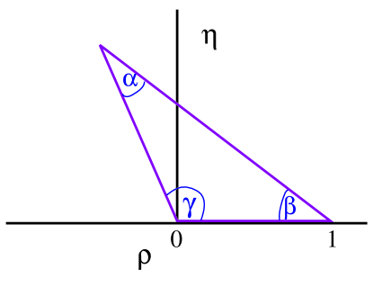
Figure 1: Unitarity Triangle for CKM elements.

The CKM matrix must be unitary and the relation between elements of different rows dictated by this property can be graphically represented as so called ‘unitarity triangles’. Fig. 1 shows one of the triangles where all the angles are expected to be large: the angles $\alpha$, $\beta$ and $\gamma$ are all related to the single phase in the $CKM$ matrix element. The study of $B$ decays will eventually allow the measurements of all the three angles. Additional constraints on the sides will be available too, through more precise measurements of $V_{ub}/V_{cb}$ and the determination of the $B^{o}_{s}\overline{B}^{o}_{s}$ mixing parameter $x_{s}$.

In parallel, the study of rare decays can provide a window beyond the Standard Model, through a detailed comparison of measured and expected branching fractions. This study needs a refined understanding of strong interaction effects, but may provide powerful constraints on a wide spectrum of models that try to address some of the shortcomings of the Standard Model.

2 Rare Decays

Rare $b$ decays encompass several different final states. In general their common feature is that their dominant decay diagram is based on a suppressed mechanism, either because it is a higher order term in a series expansion (e.g. loops in the so called ‘penguin’ diagrams) or because the quark coupling at the decay vertex is CKM suppressed.

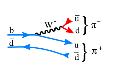
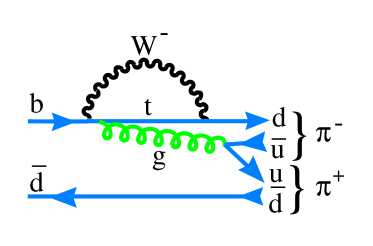
Figure 2: Feynman Diagrams for the decay $B^{0}\rightarrow\pi^{+}\pi^{-}$.

There are several reasons why a precise experimental mapping of the phenomenology of rare $b$ decays is very important. First of all the decay amplitude suppression makes it possible for these Standard Model processes to interfere with decay diagrams mediated by exotic mechanisms due to ‘beyond Standard Model’ interactions. In addition, loop diagrams and CKM suppression can affect our ability of measuring CP violation phases in two different ways. On one hand, loops and CKM suppressed diagrams can lead to final states accessible to both $B$ and $\overline{B}$ decays, making it possible to measure interference effects even without neutral $B$ mixing. On the other hand, the interplay between these two processes can cloud the relationship between measured $CP$ asymmetries and the CKM phase when mixing induced CP violation is looked for. A classical example of this effect is the decay $B^{o}\rightarrow\pi^{+}\pi^{-}$. The two Standard Model diagrams contributing to this decay process are shown in Fig. 2. If the $b\rightarrow u$ diagram is dominant, the angle $\alpha$ can be extracted from the measurement of the asymmetry in the decay $B^{o}\rightarrow\pi^{+}\pi^{-}$. On the other hand, if these two diagrams have comparable amplitude, the extraction of $\alpha$ from this decay channel is going to be a much more difficult task.

CLEO has studied several decays that can lead to a more precise understanding of the interplay between penguin diagrams and $b\rightarrow u$ diagrams in $B$ meson decays. The analysis technique used has been extensively refined in order to make the best use of the limited statistics presently available. In most of the decay channels of interest, the dominant source of background are continuum events; the fundamental difference between $e^{+}e^{-}\rightarrow q\overline{q}$ and $B$ decays is the shape of the underlying event. The latter decays tend to produce a more ‘spherical’ distribution of particles whereas continuum events tend to be more ‘jet-like’, with most of the particle emitted into two narrow back to back ‘jets’. This property can be translated into several different shape variables. CLEO constructs a Fisher discriminant ${\cal F}=\Sigma_{i}\alpha_{i}y_{i}$, a linear combination of several variables $y_{i}$. The variables used are $|\cos{\theta_{cand}}|$, the cosine of the angle between the candidate $B$ sphericity axis and the beam axis, the ratio of Fox-Wolfram moments $R_{2}=H_{2}/H_{0}$, and nine variables that measure the scalar sum of the momenta of the tracks and showers from the rest of the event in 9 angular bins, each of 10^∘, around the candidate sphericity axis. The coefficients $\alpha_{i}$ have been chosen to optimize the separation between signal and background Monte Carlo samples [2]. In addition, several kinematical constraints allow a more precise determination of the final state. First of all the energy difference $\Delta E=E_{cand}-E_{B}$, where $E_{cand}$ is the reconstructed candidate mass and $E_{B}$ is the known beam energy ($\Delta E=0$ for signal events) and the beam constrained mass $M$. In addition, the $B$ decay angle with respect to the beam axis has a $\sin^{2}(\theta_{B})$ angular distribution. Finally, to improve the separation between the final states $K\pi$ and $\pi\pi$ the specific energy loss in the drift chamber, $dE/dx$ is used.

CLEO uses a sophisticated unbinned maximum likelihood (ML) fit to optimize the precision of the signal yield obtained in the analysis, using $\Delta E$, $M$, ${\cal F}$, $|\cos{\theta_{B}}|$, and $dE/dx$ wherever applicable . In each of these fits the likelihood of the event is parameterized by the sum of probabilities for all the relevant signal and background hypotheses, with relevant weights determined by maximizing the likelihood function (${\cal L}$). The probability of a particular hypothesis is calculated as the product of the probability density functions for each of the input variables determined with high statistics Monte Carlo samples. The likelihood function is defined as:

$${\cal L}=\Pi_{k}\Sigma_{i}P^{i}_{k}(\Delta E,M_{B},{\cal F},dE/dx,\cos{\theta_{B}})\times f_{i}$$ (3)

where the index $k$ runs over the number of events, the index $i$ over the hypotheses considered, $P^{i}_{k}$ are the probabilities for different hypotheses obtained from Monte Carlo simulations of the signal and background channels considered and independent data samples, and $f_{i}$ are the fractional yields for hypothesis $i$, with the constraint:

$$\Sigma_{i}f_{i}=1$$ (4)

Further details about the likelihood fit can be found elsewhere [2]. The fits include all the decay channels having a similar topology. For example, in the final state including two charged hadrons, the final states considered were $K^{\pm}\pi^{\mp}$, $\pi^{\pm}\pi^{\mp}$ and $K^{\pm}K^{\mp}$.

Fig. 3 shows contour plots of the ML fits for the signal yields in the $K^{\pm}\pi^{\mp}$ and $\pi^{\pm}\pi^{\mp}$ final states. The other channels included in the likelihood function have $f_{i}$ fixed to their most probable value extracted from the fit. It can be seen that there is a well defined signal for the $K^{\pm}\pi^{\mp}$ final state, whereas there is less than 3$\sigma$ evidence of having seen $\pi^{+}\pi^{-}$. This shows that the $b\rightarrow u$ diagram is suppressed with respect to the penguin diagram in $B$ decays to two pseudoscalar mesons. Table 1 summarizes the CLEO results for the $B\rightarrow K\pi,~{}\pi\pi,~{}KK$ final states. Unless explicitly stated, the results are based on a data sample of 5.8 million $B\overline{B}$ pairs. There is a consistent pattern of penguin dominance in $B$ decays into two charmless pseudoscalar mesons that makes the prospects of extracting the angle $\alpha$ from the study of the CP asymmetry in the $B\rightarrow\pi\pi$ mode less favorable than originally expected.

Figure 3: $n\sigma$ contours for $B^{o}\rightarrow h^{+}\pi^{-}$, corresponding to an increase of $-2\ln{\cal L}$ by $n^{2}$. The cross identifies the most probable values of the $\pi^{+}pi^{-}$ and $K^{+}\pi^{-}$ yields.

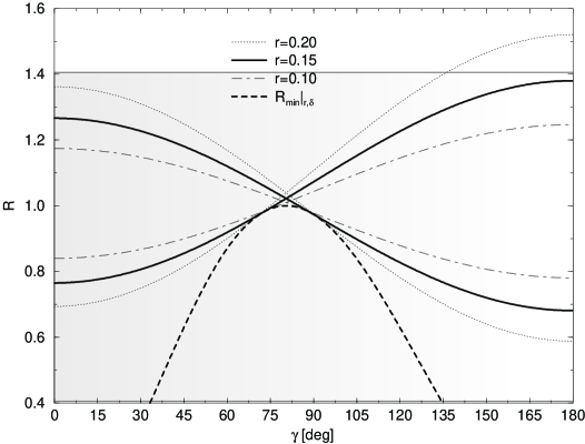
Figure 4: The dependence of the extremal values of $R_{FM}$ on the CKM angle $\gamma$ in the case of negligible rescattering effects [5]; $r=\mid T\mid/\sqrt{<\mid P\mid^{2}>}$, where $T$ is the “tree” amplitude and $P\equiv{\cal A}(B^{+}\rightarrow\pi^{+}K^{o})$, and $R_{min}\mid_{r\delta}$ is the minimal value of $R_{FM}$.

Recently a lot of theoretical discussion has been focused on the possibility of extracting the angle $\gamma$ from the study of a variety of ratios of the decays just reviewed. Originally Fleisher and Mannel [3] proposed to consider the ratio

$$R_{FM}=\frac{{\cal B}(B^{o}\rightarrow K^{+}\pi^{-})}{{\cal B}(B^{+}\rightarrow K^{o}\pi^{+})}$$ (5)

Subsequently Neubert and Rosner [4] proposed a different ratio:

$$R_{NR}=\frac{{\cal B}(B^{+}\rightarrow K^{o}\pi^{+})}{2{\cal B}(B^{+}\rightarrow K^{+}\pi^{o})}$$ (6)

A careful study of the effects of final state interaction is necessary to evaluate the relationship between these two ratios and $\gamma$ [5], [7]. The CLEO result for these ratios is:

$$R_{FM} = 0.9\pm 0.4\pm 0.2\pm 0.2$$ (7)

$$R_{NR} = 0.47\pm 0.21\pm 0.12$$ (8)

The last error in $R_{FM}$ is due to the uncertainty in the charged to neutral $B$ meson ratio at the $\Upsilon(4{\rm S})$ ($f_{\pm}/f_{oo}=1.15\pm 0.17\pm 0.06$) [6]. The experimental errors are too big to be able to exclude specific $\gamma$ intervals, but Fig. 4 shows that a more precise measurement could restrict the allowed $\gamma$ regions.

Table 1: Summary of CLEO results for $B\rightarrow K\pi,\pi\pi,KK$.

Mode	Yield	${\cal B}$/U.L. (x10-5)	Theory (10-5)[8]
$K^{+}\pi^{-}$	$43.1^{+9.0}_{-8.2}$	$1.4\pm 0.3\pm 0.2$	1.4 -1.8
$K^{+}\pi^{o}$	$38.1^{+9.7}_{-8.7}$	$1.5\pm 0.4\pm 0.3$	0.9 - 1.2
$K^{o}\pi^{-}$	$12.3^{+4.7}_{-3.9}$	$1.4\pm 0.5\pm 0.2$	1.4 -2.2
$\pi^{+}\pi^{-}$	$11.5^{+6.3}_{-5.2}$	$<0.84$	0.9 -1.2
$\pi^{+}\pi^{o}$	$14.9^{+8.1}_{-6.9}$	$<1.6$	0.3 -0.7
$K^{+}K^{-}$	$0.0^{+1.6}_{-0.0}$	$<0.23$	0.3 -0.7
$K^{+}K^{o}$	$1.8^{+2.6}_{-1.4}$	$<0.93$	0.3 -0.6
Published Results based on $3.3\times 10^{6}B\overline{B}$ pairs
$K^{o}\pi^{o}$	$4.1^{+3.1}_{-2.4}$	$<4.1$	0.5 -0.7
$\pi^{o}\pi^{o}$	$2.7^{+2.7}_{-1.7}$	$<0.93$	0.3-0.6
$K^{o}\overline{K}^{o}$	0	$<1.7$	0.1 -0.8

The CLEO study of $B$ decays to final states including two charmless hadrons has presented some other interesting surprises. A large branching ratio has been discovered for final states including a $\eta^{\prime}$ meson. The analysis technique in this case is essentially the same as the one discussed above. The $\eta^{\prime}$ is reconstructed both in its $\eta\pi^{+}\pi^{-}$ and $\rho\gamma$ decay channels. The results for different decay modes including $\eta$ and $\eta^{\prime}$ are summarized in Table 2. The most notable feature of these results is the astonishing large rate for the $\eta^{\prime}K$ final state. While several theoretical interpretations have been proposed to explain this enhancement [9], a very plausible explanation is still pointing to a dominance of penguin effects in $B$ decays into two pseudoscalar charmed hadrons.

Table 2: Summary of CLEO results for $B\rightarrow\eta^{\prime}\pi/K,\eta\pi/K$.

Mode	Yield	${\cal B}$/U.L. (x10-5)	Theory (10-5)[8]
$\eta^{\prime}K^{+}$	$68.6$	$7.4^{+0.8}_{-1.3}\pm 1.0$	2.1-3.5
$\eta^{\prime}K^{o}$	$18.1$	$5.9^{+1.8}_{-1.6}\pm 0.9$	2.0-3.5
$\eta^{\prime}\pi^{+}$	1.0	$<1.2$	1.1-2.7
$\eta K^{+}$	1.3	$<1.4$	0.2-0.4
$\eta\pi^{+}$	0.2	1.5	0.2-0.2

Table 3: Summary of CLEO results for $\overline{B}^{o}/B^{-}\rightarrow\rho\pi/K$ (in units of $10^{-5})$

	$\rho^{-}\pi^{+}$	$\rho^{+}\pi^{-}$	$\rho^{-}\pi^{0}$	$\rho^{o}\pi^{-}$	$\rho^{o}\pi^{o}$
CLEO ${\cal B}$/U.L. )	$3.5^{+1.1}_{-1.0}\pm 0.5$		$<7.7$	$1.5\pm 0.5\pm 0.4$	$<1.8$
Ciuchini et al.[10]	1.0-7.5	0.2-1.9	0.3-2.6	0.5-1.1	0.0-0.2
Ali et al.[8]	2.1-3.4	0.6-0.9	1.1 -1.6	0.1-0.7	0.0-0.2

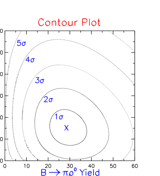
Figure 5: $n\sigma$ contours for the decays $B^{+}\rightarrow\rho^{0}\pi^{+}$ and $B^{+}\rightarrow\rho^{0}K^{+}$. The cross identifies the most probable values of the yields for these two channels.

The results discussed so far are quite discouraging for our prospects of studying $b\rightarrow u$ transitions in charmless hadronic $B$ decays. Luckily recent CLEO data suggest that final states involving a vector and a psedoscalar meson offer a different picture. In fact, the first observation of $B^{+}\rightarrow\pi^{+}\rho^{o}$ and $B\rightarrow\rho^{\pm}\pi^{\mp}$[11]. They are also first observations of $b\rightarrow u$ hadronic transitions. The analysis procedure is similar to the one adopted for other charmless exclusive decays. In this case, there are three particles in the final state and some additional constraints are provided by the vector particle decay kinematics. The invariant mass of its decay products must be consistent with the vector meson mass. In addition, the vector meson is polarized, thus its helicity angle $\theta_{h}$ is expected to have a $\cos^{2}{\theta_{h}}$ distribution. In this case the maximum likelihood fit includes $\pi\rho^{0}$ and $K\rho^{0}$ signal channels and continuum samples. The $n\ \sigma$ contour plot for this analysis is shown in Fig. 5 and gives solid evidence for a $B^{+}\rightarrow\pi^{+}\rho^{o}$ signal, while in this case the $B^{+}\rightarrow K^{+}$ channel appears to be suppressed. Other $b\rightarrow u$ modes with $B\rightarrow PV$ topology have been searched: the measured upper limits are very close to the theoretical predictions, as shown in Table 3. Thus, hopefully, more positive signals can be measured soon, when the full CLEO II.5 data set will be processed.

3 Inclusive $\eta^{\prime}$ production

A deeper understanding of the dynamics of the gluonic penguin process $b\rightarrow sg$ is quite important as it is expected to play a critical role in direct CP violation in B decays [12]. As mentioned above, this process appears to be the dominant decay mechanism in $B$ decays into two charmless pseudoscalar mesons. The inclusive $B\rightarrow\eta^{\prime}X_{s}$ signal, where the $X$ represents a collection of particles containings a single $s$ quark, is a possible signature of $b\rightarrow sg^{\star},g^{\star}\rightarrow gu\overline{u},d\overline{d}\ {\rm or}\ s\overline{s}$.

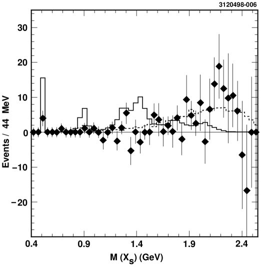
Figure 6: The continuum subtracted $M(X_{s})$ distribution (points with error bars) with expected $M(X_{s})$ distribution for a mixture of two body $b\rightarrow sq\overline{q}$ (solid) and three-body $b\rightarrow sg^{\star}$ with $g^{\star}\rightarrow g\eta^{\prime}$ simulated with JETSET (dashed). The data points have been corrected for $M(X_{s})$ dependent efficiency. Each simulation has been normalized to the data yield.

In searching for $B\rightarrow\eta^{\prime}X_{s}$, we focus on the end point of the $\eta^{\prime}$ spectrum, to suppress contributions from $b\rightarrow c$ processes. In this analysis the momentum window is chosen to be $2.0GeV/c~{}<p_{\eta^{\prime}}<2.7~{}GeV/c$. The analysis technique is similar to the one that lead to a successful measurement of the inclusive $b\rightarrow s\gamma$ process, explicitly reconstructing the $X_{s}\rightarrow\eta^{\prime}K^{\pm}n\pi$, where $n\leq 4$ and at most 1 $\pi^{o}$ is included. This pseudo-exclusive reconstruction technique is quite effective in suppressing continuum background. Upon continuum subtraction an excess yield is found. Fig. 6 shows the $X_{s}$ mass spectrum compared with different Monte Carlo shapes obtained with two different hypotheses for the source of this excess: $b\rightarrow sq\overline{q}$ and $b\rightarrow sg^{\star}$. The mass spectrum clearly favors a $b\rightarrow sg^{\star}$ origin. Several alternative hypotheses have been investigated as an explanation of this excess [13], but all the features of the data seem to favor the $b\rightarrow sg^{\star},~{}g^{\star}\rightarrow g\eta^{\prime}$ hypothesis.

The branching fraction corresponding to this excess is:

$${\cal B}(B\rightarrow\eta^{\prime}X_{s})=(6.2\pm 1.6\pm 1.3^{+0.0}_{-1.5})\times 10^{-4}\ (2.0~{}GeV/c<p_{\eta^{\prime}}<2.7~{}GeV/c)$$ (9)

This measured $\eta^{\prime}$ production is probably too large compared to conventional calculations of the hadronic matrix element for the penguin operator [14]. Explanations for this anomaly are similar to the ones proposed for the enhancement in exclusive modes discussed above [15]. A more precise theoretical evaluation of the hadronic matrix element is necessary before we can advocate new physics to understand this excess.

4 Final state interaction phases

Different final state interaction phases are a necessary ingredient, as well as different weak interaction phases, to lead to the interference that produces direct CP asymmetries. A way to identify final state interaction effects is to search for phase differences in decays into two vector states. This information is obtained by performing a full angular distribution analysis of such decays.

The formalism and analysis technique will be discussed with reference to the decay $B\rightarrow D^{\star}\rho$, the mode studied most recently [16]. While the charged $B$ decay is mediated both by a spectator and color suppressed diagram, only the spectator diagram is expected to contribute to the neutral $B$ decay. Thus interference effects in the latter decay are an unambiguous sign of final state interaction.

The angular distribution for $B\rightarrow D^{\star}\rho$ is described in terms of three helicity amplitudes, $H_{\pm,o}$:

$$\frac{32\pi}{9\Gamma}\frac{d^{3}\Gamma}{d\cos{\theta_{1}}d\cos{\theta_{2}}d\chi}=$$ (10)

$$4\mid H_{o}\mid^{2}\cos^{2}{\theta_{1}}\cos^{2}{\theta_{2}}+(\mid H_{+}\mid^{2}+\mid H_{\mid}^{2})\sin^{2}{\theta_{1}}\sin^{2}{\theta_{2}}+$$

$$[{\cal R}(H_{-}H^{\star}_{+})\cos{2\chi}+{\cal I}(H_{-}H^{\star}_{+})\sin{2\chi}]2\sin^{2}{\theta_{1}}\sin^{2}{\theta_{2}}+$$

$$[{\cal R}(H_{-}H^{\star}_{o}-H_{+}H^{\star}_{o})\cos{\chi}+{\cal I}(H_{-}H^{\star}_{o}-H_{-}H^{\star}_{o})\sin{\chi}]\sin{2\theta_{1}}\sin{2\theta_{2}}\sin^{2}{\theta_{2}},$$

where $\theta_{1}$ is the $D^{0}$ angle in the $D^{\star}$ rest frame, $\theta_{2}$ is the $\pi^{+}$ angle in the $\rho$ rest frame and $\chi$ is the angle between the $D^{\star}$ and the $\rho$ decay planes in the $B$ rest frame. Assuming $CP$ symmetry in the decay, the helicity amplitudes of the $B$ and $\overline{B}$ are related:

$$H_{\lambda}(\overline{B})=H_{-\lambda}(B)\ (\lambda=+,-,0).$$ (11)

This corresponds to flipping the sign of $\chi$. The two data sets are combined accordingly. Furthermore, the phases are measured with respect to $H_{o}$ and the normalization condition is:

$$\mid H_{o}\mid^{2}+\mid H_{+}\mid^{2}+\mid H_{-}\mid^{2}=1$$ (12)

This makes the angular distribution invariant under the exchange $H_{\pm}\leftrightarrow H^{\star}_{\mp}$, thus making the distinction between $H_{+}$ and $H_{-}$ arbitrary. Because of the $V-A$ nature of the interaction, $H_{-}$ is assumed to be the larger of the two for $\overline{B}$. Table 4 shows the fit results. There are signs of non-zero phases. The angular distribution in Eq. 10 would imply that non-trivial phases should result in asymmetric $\chi$ angular distributions. The data do not show such an asymmetry, probably because of limited statistics. The measured non-zero phases are an interesting indication that another ingredient necessary to see CP violation, final state interaction, indeed exists.

Table 4: Fit results for helicity amplitudes. The phase and magnitude of the amplitudes $H_{+}$ and $H_{-}$ are measured with respect to $H_{o}$.

$B^{o}\rightarrow D^{\star-}\rho^{+}$	Magnitude	Phase
$H_{o}$	0.936	0
$H_{-}$	$0.317\pm 0.052\pm 0.013$	$0.19\pm 0.23\pm 0.14$
$H_{+}$	$0.152\pm 0.058\pm 0.037$	$1.47\pm 0.37\pm 0.32$
$B^{+}\rightarrow D^{\star o}\rho^{+}$	Magnitude	Phase
$H_{o}$	0.932	0
$H_{-}$	$0.283\pm 0.068\pm 0.039$	$1.13\pm 0.27\pm 0.17$
$H_{+}$	$0.228\pm 0.069\pm 0.036$	$0.95\pm 0.31\pm 0.19$

5 Conclusion

We have reviewed several results on hadronic $B$ decays that are closely related to the search for direct and mixing mediated CP violation. In particular, the role of gluonic penguins and final state interaction in these decays has been investigated extensively. These measurements represent an important step in our goal of a precise determination of the CKM parameters.

6 Acknowledgements

I would like to thank Mario Greco, Giorgio Bellettini and Giorgio Chiarelli for a very pleasurable and thought provoking conference. Many thanks to all my colleagues in CLEO that have made it possible for me to present this wide spectrum of interesting data. Lastly I would like to thank Sheldon Stone for several interesting discussions, Frank Würthwein and Tomasz Skwarnicki for useful suggestions. This work was supported by NSF.

References

- [1] L. Wolfenstein, Phys. Rev. Lett. 51, 1945 (1983).
- [2] D. M. Asner et al. (CLEO Collaboration), Phys. Rev. D53, 1039 (1996).
- [3] R. Fleischer and T. Mannel, Phys. Rev D57, 2752 (1997)
- [4] M. Neubert and J. Rosner, Phys. Rev. Lett. 81, 5076 (1988).
- [5] A. Buras and R. Fleischer, CERN Preprint CERN-TH-98-319, (1998).
- [6] S. Schuh and S.Stone, Contributed Paper to the Centennial APS Meeting, Atlanta, GA (1999).
- [7] M. Neubert, JHEP 9902, 14 (1999).
- [8] A. Ali, G. Kramer, and C.D. Lu, Phys. Rev. D58, 094009 (1998).
- [9] A sample of the various theories proposed can be found in: I. Halperin and A. Zhitnitsky, Phys. Rev. D56, 7247 (1997); F. Yuan and K.T. Chao, Phys. Rev. D56, 2495 (1997); D. Atwood and A. Soni Phys. Lett. B405, 150 (1997).
- [10] M. Ciuchini et al. , Nucl. Phys. B51 3 (1998).
- [11] Y. Gao, F. Würthwein (CLEO Collaboration), Caltech Preprint CALT 68 - 2220/ Harvard Preprint HUTP-99/A021, 1999.
- [12] X. He, W.S. Hou and K.C. Yang, Phys. Rev. Lett. 81, 5738 (1998).
- [13] T.E. Browder et al. (CLEO Collaboration), CLEO CONF 98-02 ICHEP98-857, 1998.
- [14] A. Datta, X.G. He and S. Pakvasa, Phys. Lett. B419, 369 (1998).
- [15] B. H. Behrens et al. (CLEO Collaboration), CLEO CONF 98-09, ICHEP98-860, 1998.
- [16] G. Bonviciniet al. (CLEO Collaboration), CLEO CONF 98-23 ICHEP98-852, 1998.