Transverse spectra of induced radiation are discussed within the light-cone path integral approach to the LPM effect. The results are applicable in both QED and QCD.

Recently the Landau-Pomeranchuk-Migdal (LPM) effect [1, 2] in induced radiation in QED and QCD has attracted much attention (see review by Klein [3] and references therein). Understanding the LPM effect in QCD is of great importance for evaluation of parton energy loss in nuclei and a hot QCD medium [4, 5, 6, 7, 8]. The case of hot QCD medium is especially interesting in view of the experiments on $AA$-collisions at RHIC and LHC.

In Ref. [5] I have developed a new rigorous light-cone path integral approach to the LPM effect. There I have discussed the $p_{\perp}$-integrated spectra. In this talk I discuss the transverse spectra of induced radiation. Similarly to Ref. [5] the results are applicable in both QED and QCD. For simplicity I describe the formalism for an induced $a\rightarrow bc$ transition in QED for scalar particles with an interaction Lagrangian $L_{int}=\lambda[\hat{\psi}_{b}^{+}\hat{\psi}_{c}^{+}\hat{\psi}_{a}+\hat{\psi}_{b}\hat{\psi}_{c}\hat{\psi}_{a}^{+}]$. The corresponding $S$-matrix element reads

$$\langle bc|\hat{S}|a\rangle=i\int\!dtd\mbox{{\bf r}}\lambda\psi_{b}^{*}(t,\mbox{{\bf r}})\psi_{c}^{*}(t,\mbox{{\bf r}})\psi_{a}(t,\mbox{{\bf r}})\,,$$ (1)

where $\psi_{i}$ are the wavefunctions (ingoing for $i=a$ and outgoing for $i=b,c$). I normalize the flux to unity at $z=-\infty$ for $i=a$ and at $z=\infty$ for $i=b,c$, and write $\psi_{i}$ as

$$\psi_{i}(t,\mbox{{\bf r}})=\frac{1}{\sqrt{2E_{i}}}\exp[-i(t-z)p_{i,z}]\phi_{i}(t,\mbox{{\bf r}})\,.$$ (2)

In the high energy limit, $E_{i}\gg m_{i}$, the dependence of $\phi_{i}$ on the variable $\tau=(t+z)/2$ at $t-z=$const is governed by the two-dimensional Schrödinger equation

$$i\frac{\partial{\phi_{i}}}{\partial{\tau}}=H_{i}\phi_{i}\,,$$ (3)

$$H_{i}=-\frac{\Delta_{\perp}}{2\mu_{i}}+e_{i}A^{0}+\frac{m_{i}^{2}}{2\mu_{i}}\,,$$ (4)

where $\mu_{i}=p_{i,z}$, $e_{i}$ is the electric charge, $A^{0}$ is the potential of the target.

After some algebra from (1), (2) one can obtain in the high energy limit the following expression for the inclusive probability of induced radiation

$$\frac{d^{5}P}{dxd\mbox{{\bf q}}_{b}d\mbox{{\bf q}}_{c}}=\frac{2}{(2\pi)^{4}}\mbox{Re}\!\int\limits_{z_{1}<z_{2}}\!d\mbox{{\boldmath$\rho$}}_{1}d\mbox{{\boldmath$\rho$}}_{2}dz_{1}dz_{2}\,g\langle F(z_{1},\mbox{{\boldmath$\rho$}}_{1})F^{*}(z_{2},\mbox{{\boldmath$\rho$}}_{2})\rangle\,,$$ (5)

where $\mbox{{\bf q}}_{b,c}$ are the transverse momenta, $\rho$ is transverse coordinate, $x=p_{b,z}/p_{a,z}$ (note that for the particle $c$ $p_{c,z}=(1-x)p_{a,z}$), $g=\lambda^{2}/[16\pi x(1-x)E_{a}^{2}]$, $\langle...\rangle$ means averaging over the states of the target, $\left.F(z,\mbox{{\boldmath$\rho$}})=\phi_{b}^{*}(t,\mbox{{\bf r}})\phi_{c}^{*}(t,\mbox{{\bf r}})\phi_{a}(t,\mbox{{\bf r}})\right|_{t=z}$. Since the wavefunctions enter (5) only at $t=z$, $\phi_{i}$ can be regarded as functions of $z$, and $\rho$. In the Schrödinger equation (3) $z$ will play the role of time. I represent $z$-dependence of $\phi_{i}$ in terms of the Green’s function, $K_{i}$, of the Hamiltonian (4). Then, in the diagram language (5) is described by the graph of Fig. 1a. I depict $K_{i}$ ($K_{i}^{*}$) by $\rightarrow$ ($\leftarrow$). The dotted line shows the transverse density matrices at large longitudinal distances in front of ($z=z_{i}$) and behind ($z=z_{f}$) the target. If the particle $a$ is produced in a hard reaction, and does not propagate from infinity, then $z_{i}$ equals the coordinate of the production point.

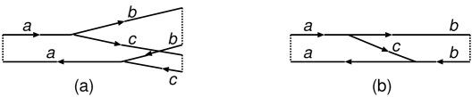
Figure 1: The diagram representation of the inclusive spectrum (5) (a), and (6) (b).

Below I will consider the radiation rate integrated over $\mbox{{\bf q}}_{c}$. In this case the graph of Fig. 1a is transformed into the one of Fig. 1b. The corresponding analytical expression reads

$$\frac{d^{3}P}{dxd\mbox{{\bf q}}_{b}}=\frac{2}{(2\pi)^{2}}\mbox{Re}\int\limits_{z_{i}}^{z_{f}}\!dz_{1}\int\limits_{z_{1}}^{z_{f}}\!dz_{2}\int\!d\mbox{{\boldmath$\rho$}}_{b,f}d\mbox{{\boldmath$\rho$}}_{b,f}^{{}^{\prime}}d\mbox{{\boldmath$\rho$}}_{b}d\mbox{{\boldmath$\rho$}}_{b}^{{}^{\prime}}d\mbox{{\boldmath$\rho$}}_{a}d\mbox{{\boldmath$\rho$}}_{a}^{{}^{\prime}}d\mbox{{\boldmath$\rho$}}_{a,i}d\mbox{{\boldmath$\rho$}}_{a,i}^{{}^{\prime}}\,g\exp[-i\mbox{{\bf q}}_{b}(\mbox{{\boldmath$\rho$}}_{b,f}-\mbox{{\boldmath$\rho$}}_{b,f}^{{}^{\prime}})]$$

$$\times S_{b}(\mbox{{\boldmath$\rho$}}_{b,f},\mbox{{\boldmath$\rho$}}_{b,f}^{{}^{\prime}},z_{f}|\mbox{{\boldmath$\rho$}}_{b},\mbox{{\boldmath$\rho$}}_{b}^{{}^{\prime}},z_{2})M(\mbox{{\boldmath$\rho$}}_{b},\mbox{{\boldmath$\rho$}}_{b}^{{}^{\prime}},z_{2}|\mbox{{\boldmath$\rho$}}_{a},\mbox{{\boldmath$\rho$}}_{a}^{{}^{\prime}},z_{1})S_{a}(\mbox{{\boldmath$\rho$}}_{a},\mbox{{\boldmath$\rho$}}_{a}^{{}^{\prime}},z_{2}|\mbox{{\boldmath$\rho$}}_{a,i},\mbox{{\boldmath$\rho$}}_{a,i}^{{}^{\prime}},z_{i})\,,\,\,\,\,\,\,\,\,\,\,\,\,\,\,\,\,$$ (6)

$$S_{i}(\mbox{{\boldmath$\rho$}}_{2},\mbox{{\boldmath$\rho$}}_{2}^{{}^{\prime}},z_{2}|\mbox{{\boldmath$\rho$}}_{1},\mbox{{\boldmath$\rho$}}_{1}^{{}^{\prime}},z_{1})=\langle K_{i}(\mbox{{\boldmath$\rho$}}_{2},z_{2}|\mbox{{\boldmath$\rho$}}_{1},z_{1})K_{i}^{*}(\mbox{{\boldmath$\rho$}}_{2}^{{}^{\prime}},z_{2}|\mbox{{\boldmath$\rho$}}_{1}^{{}^{\prime}},z_{1})\rangle\,,$$ (7)

$$M(\mbox{{\boldmath$\rho$}}_{2},\mbox{{\boldmath$\rho$}}_{2}^{{}^{\prime}},z_{2}|\mbox{{\boldmath$\rho$}}_{1},\mbox{{\boldmath$\rho$}}_{1}^{{}^{\prime}},z_{1})=\langle K_{b}(\mbox{{\boldmath$\rho$}}_{2},z_{2}|\mbox{{\boldmath$\rho$}}_{1},z_{1})K_{c}(\mbox{{\boldmath$\rho$}}_{2}^{{}^{\prime}},z_{2}|\mbox{{\boldmath$\rho$}}_{1},z_{1})K_{a}^{*}(\mbox{{\boldmath$\rho$}}_{2}^{{}^{\prime}},z_{2}|\mbox{{\boldmath$\rho$}}_{1}^{{}^{\prime}},z_{1})\rangle\,.$$ (8)

Using the path integral representation for the Green’s functions one can evaluate analytically the initial- and final-state interaction factors $S_{a,b}$ [9]. The factor $M$ (8) differs from that of Ref. [5] by the replacement of $\mbox{{\boldmath$\rho$}}_{2}^{{}^{\prime}}$ by $\mbox{{\boldmath$\rho$}}_{2}$ in the Green’s function $K_{c}$. Similar to that of Ref. [5] it can be expressed through the Green’s function $K_{bc}$ describing the relative motion of the particles $b$ and $c$ in a fictitious $\bar{a}bc$ system. After analytical integration over the center-of-mass transverse coordinates the radiation rate takes the form

$$\frac{d^{3}P}{dxd\mbox{{\bf q}}_{b}}=\frac{2}{(2\pi)^{2}}\mbox{Re}\int\limits_{z_{i}}^{z_{f}}\!dz_{1}\int\limits_{z_{1}}^{z_{f}}\!dz_{2}\int\!d\mbox{{\boldmath$\tau$}}_{b}\,g\exp(-i\mbox{{\bf q}}_{b}\mbox{{\boldmath$\tau$}}_{b})$$

$$\times\Phi_{b}(\mbox{{\boldmath$\tau$}}_{b},z_{2})\exp\left[\frac{i(z_{1}-z_{2})}{L_{f}}\right]K_{bc}(\mbox{{\boldmath$\tau$}}_{b},z_{2}|0,z_{1})\Phi_{a}(\mbox{{\boldmath$\tau$}}_{a},z_{1})\,,$$ (9)

where

$$\Phi_{a}(\mbox{{\boldmath$\tau$}}_{a},z_{1})=\exp\left[-\frac{\sigma_{a\bar{a}}(\mbox{{\boldmath$\tau$}}_{a})}{2}\int\limits_{z_{i}}^{z_{1}}\!dzn(z)\right]\,,\,\,\,\,\,\,\,\,\Phi_{b}(\mbox{{\boldmath$\tau$}}_{b},z_{2})=\exp\left[-\frac{\sigma_{b\bar{b}}(\mbox{{\boldmath$\tau$}}_{b})}{2}\int\limits_{z_{2}}^{z_{f}}\!dzn(z)\right]$$ (10)

are the eikonal initial- and final-state absorption factors, $\mbox{{\boldmath$\tau$}}_{a}=x\mbox{{\boldmath$\tau$}}_{b}$, $L_{f}=2E_{a}x(1-x)/[m_{b}^{2}(1-x)+m_{c}^{2}x-m_{a}^{2}x(1-x)]$. The Hamiltonian for the Green’s function $K_{bc}$ reads

$$H_{bc}=-\frac{\Delta_{\perp}}{2\mu_{bc}}-\frac{in(z)\sigma_{\bar{a}bc}(\mbox{{\boldmath$\tau$}}_{bc},\mbox{{\boldmath$\tau$}}_{ab})}{2}\,,$$ (11)

where $\mu_{bc}=E_{a}x(1-x)$, $\mbox{{\boldmath$\tau$}}_{ab}=-[\mbox{{\boldmath$\tau$}}_{a}+\mbox{{\boldmath$\tau$}}_{bc}(1-x)]$. In (10), (11) $n(z)$ is the number density of the target, $\sigma_{a\bar{a}}$ and $\sigma_{b\bar{b}}$ are the dipole cross sections of interaction with the medium constituent of $a\bar{a}$ and $b\bar{b}$ pairs, and $\sigma_{\bar{a}bc}$ is the three-body cross section for $\bar{a}bc$-system.

The integration over $\mbox{{\bf q}}_{b}$ in (9) gives the $x$-spectrum

$$\frac{dP}{dx}=2\mbox{Re}\int\limits_{z_{i}}^{z_{f}}\!dz_{1}\int\limits_{z_{1}}^{z_{f}}\!dz_{2}\,g\exp\left[\frac{i(z_{1}-z_{2})}{L_{f}}\right]K_{bc}(0,z_{2}|0,z_{1})\,.$$ (12)

In Ref. [5] I have derived the $p_{T}$-integrated radiation rate using the unitarity connection between the probability of $a\rightarrow bc$ transition and the radiative correction to $a\rightarrow a$ transition. The latter is described by the diagram of Fig. 2a, which can be transformed into the graph of Fig. 2b, corresponding to the integral in (12). One can easy show that the diagram of Fig. 2b can also be obtained directly from that of Fig. 1b after integration over $\mbox{{\bf q}}_{b}$.

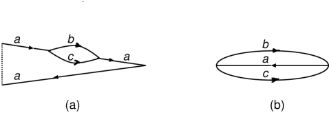
Figure 2: The diagram representation of the radiative correction to the probability of $a\rightarrow a$ transition.

Equation (9) establishes the theoretical basis for evaluation of the $p_{T}$-dependence of the LPM effect. Note that for transition with the formation length much greater than the target thickness (for the particle $a$ incident from infinity) (9) can be expressed through the light-cone wave function $\Psi_{a}^{bc}$ as

$$\frac{d^{3}P}{dxd\mbox{{\bf q}}_{b}}=\frac{2}{(2\pi)^{2}}\int\!d\mbox{{\boldmath$\tau$}}d\mbox{{\boldmath$\tau$}}^{{}^{\prime}}\exp(-i\mbox{{\bf q}}_{b}\mbox{{\boldmath$\tau$}}^{{}^{\prime}})\Psi_{a}^{bc*}(x,\mbox{{\boldmath$\tau$}}-\mbox{{\boldmath$\tau$}}^{{}^{\prime}})\Gamma_{\bar{a}bc}(\mbox{{\boldmath$\tau$}}_{bc},\mbox{{\boldmath$\tau$}}_{ab})\Psi_{a}^{bc}(x,\mbox{{\boldmath$\tau$}})\,.$$ (13)

Here, $\mbox{{\boldmath$\tau$}}_{bc}=\mbox{{\boldmath$\tau$}}$, $\mbox{{\boldmath$\tau$}}_{ab}=-[\mbox{{\boldmath$\tau$}}(1-x)+\mbox{{\boldmath$\tau$}}^{{}^{\prime}}x]$, $\Gamma_{\bar{a}bc}=\left\{1-\exp\left[-\frac{\sigma_{\bar{a}bc}}{2}\!\int\!dzn(z)\right]\right\}$ is the Glauber profile function for interaction of $\bar{a}bc$ state with the target. The derivation of (13) is based on a connection between the Green’s function $K_{bc}$ in vacuum and $\Psi_{a}^{bc}$ [10]. Equation (13) generalizes the formula for the $p_{T}$-integrated spectrum of Ref. [11]. It is of interest in its own right. In particular, the leading term in $n(z)$ of the rhs in (13) gives a convenient formula for evaluation of the Bethe-Heitler cross section through the light-cone wavefunction.

In general case one can estimate the inclusive cross section using the parametrization $\sigma_{\bar{a}bc}=C_{ab}\mbox{{\boldmath$\tau$}}_{ab}^{2}+C_{bc}\mbox{{\boldmath$\tau$}}_{bc}^{2}+C_{ca}\mbox{{\boldmath$\tau$}}_{ca}^{2}$ (here $\mbox{{\boldmath$\tau$}}_{ca}=-(\mbox{{\boldmath$\tau$}}_{ab}+\mbox{{\boldmath$\tau$}}_{bc})$). Then the Hamiltonian (11) takes the oscillator form with the frequency $\Omega(z)=\frac{(1-i)}{\sqrt{2}}\left[\frac{n(z)C(x)}{E_{a}x(1-x)}\right]^{1/2}\,,$ with $C(x)=C_{ab}(1-x)^{2}+C_{bc}+C_{ca}x^{2}$. The Green’s function for the oscillator Hamiltonian can be written in the form

$$K_{osc}(\mbox{{\boldmath$\tau$}}_{2},z_{2}|\mbox{{\boldmath$\tau$}}_{1},z_{1})=\frac{\gamma(z_{1},z_{2})}{2\pi i}\exp\left\{i\left[\alpha(z_{1},z_{2})\mbox{{\boldmath$\tau$}}_{2}^{2}+\beta(z_{1},z_{2})\mbox{{\boldmath$\tau$}}_{1}^{2}-\gamma(z_{1},z_{2})\mbox{{\boldmath$\tau$}}_{1}\mbox{{\boldmath$\tau$}}_{2}\right]\right\}\,,$$ (14)

where the functions $\alpha$, $\beta$ and $\gamma$ can be evaluated in the approach of Ref. [12]. Using the parametrization $\sigma_{\bar{i}i}=C_{ii}\mbox{{\boldmath$\tau$}}_{i}^{2}$ one can obtain

$$\frac{d^{3}P}{dxd\mbox{{\bf q}}_{b}}=\frac{1}{(2\pi)^{2}}\mbox{Re}\int\limits_{z_{i}}^{z_{f}}\!dz_{1}\int\limits_{z_{1}}^{z_{f}}\!dz_{2}\,g\,\frac{\gamma(z_{1},z_{2})}{Q(z_{1},z_{2})}\exp\left[-\frac{i\mbox{{\bf q}}^{2}_{b}}{4Q(z_{1},z_{2})}+\frac{i(z_{1}-z_{2})}{L_{f}}\right]\,,$$ (15)

where the factor $Q(z_{1},z_{2})$ can be expressed through the parameters $C_{ij}$, the functions $\alpha$, $\beta$, $\gamma$, $n$, and $\Omega$. The formula for this factor is too cumbersome to be presented here.

The generalization of the above results to the realistic QED and QCD Lagrangians reduces to a trivial replacement of the two- and three-body cross sections, and the vertex factor $g$. The latter, due to spin effects in the vertex $a\rightarrow bc$, becomes an operator. The corresponding formulas are given in Refs. [5, 13]. The results obtained can be applied to many problems. In particular in QCD this approach can be used for evaluation of high-$p_{T}$ hadron spectra, the $p_{T}$-dependence of DY pairs and heavy quarks production in $hA$-collisions, angular dependence of the parton energy loss in hot QCD matter produced in $AA$-collisions. It is also of interest for study the initial condition for quark-gluon plasma in $AA$-collisions.

I would like to thank N.N. Nikolaev and D. Schiff for discussions. I am grateful to J. Speth for the hospitality at FZJ, Jülich, where this work was completed. This work was partially supported by the INTAS grant 96-0597.

References

• [1] L.D. Landau and I.Ya. Pomeranchuk, Dokl. Akad. Nauk SSSR 92, 535, 735 (1953).
• [2] A.B. Migdal, Phys. Rev. 103, 1811 (1956).
• [3] S.R. Klein, hep-ph/9802442 (1998).
• [4] R. Baier, Yu.L. Dokshitzer, S. Peigne and D. Schiff, Phys. Lett. B345, 277 (1995).
• [5] B.G. Zakharov, JETP Lett. 63, 952 (1996).
• [6] R. Baier, Yu.L. Dokshitzer, A.H. Mueller, S. Peigne and D. Schiff, Nucl. Phys. B483, 291 (1997); B484, 265 (1997).
• [7] B.G. Zakharov, JETP Lett. 65, 615 (1997); hep-ph/9807396 (1998).
• [8] R. Baier, Yu.L. Dokshitzer, A.H. Mueller, and D. Schiff, Nucl. Phys. B531, 403 (1998).
• [9] B.G. Zakharov, Sov. J.Nucl. Phys. 46, 92 (1987).
• [10] B.G. Zakharov, JETP Lett. 64, 781 (1996).
• [11] N.N. Nikolaev, G. Piller, and B.G. Zakharov, JETP 81, 851 (1995).
• [12] B.Z. Kopeliovich and B.G. Zakharov, Phys. Rev. D44, 3466 (1991).
• [13] B.G. Zakharov, Phys. Atom. Nucl. 61, 838 (1998).