Gauge Coupling Unification with Extra Dimensions
and Gravitational Scale Effects

We study gauge coupling unification in the presence of extra dimensions compactified at a few TeV. Achieving unification requires a large number of gauge boson Kaluza-Klein excitations lighter than the string scale, such that the higher-dimensional gauge couplings are ${\cal O}(1)$ in string scale units. Corrections to the gauge couplings from two or more loops are about 10% or larger, hence string (or M) theory is generally expected to be strongly coupled in $\sim$TeV-scale extra-dimensional scenarios. Higher-dimensional operators induced by quantum gravitational effects can shift the gauge couplings by a few percent. These effects are sufficiently large that even the minimal Standard Model, or the MSSM, allow unification at a scale in the $\sim$TeV range. The strongly coupled unified theory may induce dynamical electroweak symmetry breaking.

1 Introduction

A striking feature of the observed elementary fermions is that they fit into complete $SU(5)$ representations [1]. It is therefore compelling to try to promote this $SU(5)$ to a gauge symmetry which is broken down to the Standard Model gauge group. In the usual scenario, a necessary condition is that the $SU(3)_{C}\times SU(2)_{W}\times U(1)_{Y}$ gauge couplings unify at one energy scale. The measured gauge couplings seem to be roughly converging if their logarithmic running is extrapolated over fourteen orders of magnitude in energy scale. This running is, of course, sensitive to the full elementary field content above the $M_{Z}$ scale, so that gauge coupling unification is a model dependent issue.

In the Minimal Supersymmetric Standard Model (MSSM) where superpartners have masses close to the electroweak scale, the gauge couplings converge at a grand unification (GUT) scale of $M_{\rm GUT}\sim 2\times 10^{16}$ GeV with a precision of a few percent [2, 3]. Quantitatively, given the precisely measured $SU(2)_{W}$ and $U(1)_{Y}$ couplings, requiring that the 3 gauge couplings meet exactly at one point (“naive” unification) gives a prediction of $\alpha_{3}(M_{Z})\approx 0.129$, with a mild dependence on the superpartner masses. This result is higher than the experimental average [4] $\alpha_{3}(M_{Z})\approx 0.119\pm 0.002$ by about 4 or 5 standard deviations. However, it is natural to expect some corrections of order a few percent at the GUT scale due to threshold effects [5, 3]. Allowing for such uncertainties the 3 gauge couplings of the MSSM can unify.

Are other theories disfavored if they do not unify with the same precision as the MSSM? Unfortunately, we cannot answer this question yet. Gauge coupling unification offers no observed phenomenon that measures the coupling constants at $M_{\rm GUT}$ (e.g., if proton decay is observed we will have in principle a relationship of the effective coupling constant at $M_{\rm GUT}$ to the low energy couplings and a definitive observation of the phenomenon of unification). We do not know that the couplings should meet identically at $M_{\rm GUT}$ or whether there may be other larger, decoupled effects which renormalize the couplings in unknown ways, which may imply drastically different scenarios at $M_{\rm GUT}$ than, e.g., the MSSM [6].

Recently, Dienes, Dudas and Ghergheta [7] have considered lowering the unification scale in the MSSM by allowing the gauge fields to propagate in extra dimensions which are presumed to open up at low energy scales, such as the $\sim$TeV scale [8]. Above the compactification scale of these extra dimensions, the gauge couplings depend on the energy scale as a power law, so that they converge very quickly. It is interesting that the gauge couplings still unify approximately in the presence of the extra dimensions [7, 9, 10]. It may even be possible that the unification scale is not far above the electroweak scale. In that case, the unification of the gauge couplings may have a chance to be probed directly in future experiments.

An immediate problem of a low energy unification scale is proton stability. In string theory, there can be gauge coupling unification even without the $SU(5)$ gauge symmetry, but the higher excitations of the $X$ and $Y$ gauge bosons may still be present and hence mediate proton decays with an unacceptable rate. Nevertheless, there are potentially higher dimensional theoretical solutions to this problem [7, 11]. For example, in string theory, the light fermions do not necessarily come from the same generations at the string scale. Moreover, if the quarks and leptons are localized at different points (on different branes) in the extra dimensions, then the proton decay rate can be highly suppressed.

The low-scale extra-dimensional theories are at present somewhat theoretically unconstrained. This is due to the fact that a large number of gauge invariant irrelevant (higher mass-dimension) operators can arise at the $\sim$ TeV scale and lead to a variety of effects, some of which obviate the constraints on the Standard Model. For example, Hall and Kolda [12] (see also [13]) have argued that the $S$-$T$ constraints of the oblique electroweak radiative corrections, which favor a low mass Higgs boson (and no additional chiral multiplets), disappear in the presence of certain allowed higher dimensional operators.

The present paper studies the corrections to the gauge couplings induced by the Kaluza-Klein (KK) excitations and by the higher-dimension operators which can occur in the presence of extra dimensions and a low string scale.

A key point of this paper is that, in order to achieve unification and bring the three gauge couplings together at a scale in the TeV range, there is need for many KK excitations contributing to the running. Therefore, the effective coupling constants, or equivalently the higher-dimensional gauge couplings above the compactification scale, are necessarily large. It is in fact remarkable that at the scale where the three gauge couplings appear to converge at the one-loop order, the loop expansion parameter is usually of order one, or slightly smaller. This indicates that the underlying (string or M) theory is in the non-perturbative regime, which is in agreement with a general argument that the string coupling is likely to be of order one [14]. In this case one does not know how to compute the string scale corrections to the Standard Model gauge couplings, and therefore the gauge unification is more uncertain. We adopt an effective field theory below $M_{s}$, in which there are string scale suppressed operators with coefficients of order one (or smaller if there are approximate global symmetries) determined by the non-perturbative string dynamics.

This can dramatically alter our intuition about physics beyond the low energy Standard Model. For example, in the minimal (non-supersymmetric) Standard Model it has long been argued that (1) the gauge couplings do not unify because they fail to meet at a common value by a large margin, and (2) because of the hierarchy problem, it is unlikely that we can extrapolate the gauge couplings to very high energy scales without introducing new physics at the TeV scale anyway. However, the strong dynamics at the low energy string scale in these novel scenarios offers the interesting possibility that the fundamental scale, which we take to be the string scale, $M_{s}$, is close to the electroweak scale [15, 16, 17], so that there is no hierarchy. In the end, these scenarios predict a new strong dynamics at the $\sim$TeV scale. It is therefore worthwhile to reexamine the general question of unification in the context of extra dimensions at the TeV scale and strong dynamics.

Our paper is organized as follows. In Section 2 we discuss in general the scale dependence of the $SU(3)_{C}\times SU(2)_{W}\times U(1)_{Y}$ gauge couplings in the presence of extra dimensions accessible to the gauge bosons, with a compactification scale below $M_{s}$. In Section 3 we show that any scalar field with a vacuum expectation value (VEV) modifies the gauge couplings due to certain dimension-six operators (assumed to be induced with a coefficient of order one times $M_{s}^{-2}$ by the string dynamics). In the Standard Model, the tree level shifts in the gauge couplings due to the Higgs VEV are of order $\sim\langle H\rangle^{2}/M_{s}^{2}$. A large shift, linear in $\langle\phi\rangle$, occurs when the $\phi$ scalar is an adjoint under a unified gauge group [6], or a gauge singlet. We also show that in a non-supersymmetric theory, any scalar field produces at one-loop a shift in the gauge couplings of order a few percent. Generically, the corrections to the three Standard Model gauge couplings are different, so that models in which the gauge couplings would not unify naively could in fact lead to unification in the presence of the higher-dimensional operators.

In Section 4 we present some simple examples. Since it is not known whether the non-perturbative string dynamics preserves some of the supercharges at $M_{s}$, we discuss gauge coupling unification in models with supersymmetry broken either at $M_{s}$ or at the electroweak scale. In Section 4.1 we show that the Standard Model with extra dimensions compactified at some TeV scale is consistent with gauge coupling unification at the string scale provided the inverse coupling constants receive corrections of order 5% beyond the one-loop running. Shifts of this size are naturally given by dimension-six operators involving the Higgs field and the gauge field strengths. Also we estimate the corrections to the gauge couplings from two or more loops to be of order 10% in the case of one extra dimension, and larger for more dimensions.

Since the loop expansion breaks down for more extra dimensions, it is interesting to study what non-perturbative phenomena may occur in this case. A possible effect of the non-perturbative phenomena at $M_{s}$ is chiral symmetry breaking in the quark sector. This leads to the existence of a composite Higgs sector [18], in which the scalars are made up of quarks bound together by KK excitations of the gluons. In Section 4.2 we point out that the ideas of gauge coupling unification and Higgs compositeness are perfectly compatible in the presence of extra dimensions.

In Section 4.3 we turn to supersymmetric models in extra dimensions. Supersymmetric operators induced at the string scale give corrections to the gauge couplings of order the $SU(3)_{C}\times SU(2)_{W}\times U(1)_{Y}$ invariant combinations of VEVs suppressed by the appropriate power of $M_{s}$. In the MSSM these corrections are likely to be below 1%, while in the Next-to-Minimal Supersymmetric Standard Model (NMSSM) they may be as large as 10%. Although the one-loop running gives a somewhat better convergence of the gauge couplings in the MSSM than in the Standard Model, the expansion parameters are larger and hence the perturbative series are less reliable in the MSSM. In fact, if the gauge couplings unify in the MSSM with more than one compact dimensions, then this happens in the strong coupling regime.

Section 5 includes our conclusions. In the Appendix we comment on the current bounds on the compactification and string scales from collider experiments and precision low energy data.

2 Gauge Coupling Running in Extra Dimensions

We begin with a general discussion of the running of the $SU(3)_{C}\times SU(2)_{W}\times U(1)_{Y}$ gauge couplings assuming that there are $\delta$ compact spatial dimensions of radius $R\geq{\cal O}($TeV${}^{-1})$ which are accessible to the gauge bosons.

The higher-dimensional field theory is non-renormalizable. This is a red-herring because point-like quantum field theory is no longer a good description for physics above the string scale, $M_{s}$. The effects of the compact dimensions can be described, nonetheless, in the four-dimensional Minkowski spacetime by introducing a tower of KK modes with masses between $1/R$ and $M_{s}$.

The relative normalization of the three coupling constants, $\alpha_{i}$, is, as usual, model dependent. In the $SU(5)$ GUT, $\alpha_{3}=g_{s}^{2}/(4\pi)$, $\alpha_{2}=g^{2}/(4\pi)$, and $\alpha_{1}=(5/3)g^{\prime 2}/(4\pi)$, where $g_{s}$, $g$ and $g^{\prime}$ are the usual Standard Model gauge couplings. Of course, it is not known whether the $SU(5)$ normalization is the correct one. Different normalizations may be imposed at the string level. For example, non-trivial compactifications give rise to different Kac-Moody levels for the three gauge groups [19]. Also, the $\alpha_{i}$’s are normalized differently if the $SU(3)_{C}$, $SU(2)_{W}$ and $U(1)_{Y}$ groups are associated with different branes [20]. Clearly, in order to decide that gauge coupling unification does not occur in a particular model, one would have to argue that the normalizations that lead to unification are unlikely to be given by string theory. Making such an argument does not appear to be feasible, at least for now, given that string or M theory may be in the strong coupling regime [14].

In this paper we use only the usual $SU(5)$ normalization, because this is the most natural choice. The experimental values of the inverse coupling constants in the $\overline{MS}$ scheme are [4]

$$\alpha_{1}^{-1}(M_{Z}) = 58.98\pm 0.04$$

$$\alpha_{2}^{-1}(M_{Z}) = 29.57\pm 0.03$$

$$\alpha_{3}^{-1}(M_{Z}) = 8.40\pm 0.14$$ (2.1)

The $\overline{MS}$ gauge coupling constants at a scale $\mu>1/R$ are related to the measured coupling constants at the $Z$ pole by

$$\alpha_{i}^{-1}(\mu)=\alpha_{i}^{-1}(M_{Z})-\frac{b_{i}}{2\pi}\ln\left(\frac{\mu}{M_{Z}}\right)-\frac{\tilde{b}_{i}}{2\pi}{\cal F}(\delta,R\mu)+\Delta_{i}^{\rm loops}~{}.$$ (2.2)

The $b_{i}$ ($i=1,2,3$) are the one-loop $\beta$-function coefficients of the four-dimensional zero-modes (they incorporate the threshold corrections due to particles heavier than the $Z$, such as the top quark), while the $\tilde{b}_{i}$ correspond to one KK excitation for each field propagating in extra dimensions. The function ${\cal F}(\delta,R\mu)$ sums the one-loop contributions from all the KK excitations, and $\Delta_{i}^{\rm loops}$ are the corrections from two and more loops.

Let us label the KK levels by $n\geq 1$, their masses by $M_{n}$ (with $M_{n}<M_{n+1}$), and their degeneracies by $D_{n}$. In the $\overline{MS}$ scheme,

$${\cal F}(\delta,R\mu)=\sum_{n=1}^{n(\mu)}D_{n}\ln\left(\frac{\mu}{M_{n}}\right)~{},$$ (2.3)

where $n(\mu)$ is a defined by $M_{n(\mu)}<M_{n(\mu)+1}$.

The total number of KK levels below the string scale, $n_{\rm max}$, is fixed by the value of $RM_{s}$. The KK mass levels $M_{n}<M_{s}$ are determined by the condition that the equation

$$\sum_{j=1}^{\delta}k_{j}^{2}=\left(M_{n}R\right)^{2}~{},$$ (2.4)

where $k_{j}$ are integer variables, has at least one solution. The degeneracy $D_{n}$ is the number of solutions to this equation. The total number of KK modes is given by

$$N_{\rm KK}=\sum_{n=1}^{n_{\rm max}}D_{n}~{}.$$ (2.5)

For the case of only one compact dimension of radius $R>M_{s}^{-1}$ accessible to the gauge bosons, $n_{\rm max}$ is the integer satisfying $n_{\rm max}\leq RM_{s}<n_{\rm max}+1$, the number of KK modes is $N_{\rm KK}=2n_{\rm max}$, and $D_{n}=2$. It follows that

$${\cal F}(\delta=1,RM_{s})=N_{\rm KK}\ln\left(RM_{s}\right)-2\ln\left(n_{\rm max}!\right)~{}.$$ (2.6)

For $\delta\geq 2$, the KK levels are no longer equally spaced and their degeneracies are level-dependent. Therefore, ${\cal F}(\delta\geq 2,RM_{s})$ is given by an expression similar with (2.6), but with the second term on the right-hand-side modified due to the non-uniform KK levels. In Table 1 we list the KK mass levels and degeneracies that saturate the bound ${\cal F}(\delta\geq 2,RM_{s})\begin{array}[]{c}\,\sim\vspace{-21pt}\\ <\end{array}42$ (this value is relevant for the MSSM, see Section 4.3).

	$n$	$\;1\;$	2	3	4	5	6	7	8	$9$	10	11	12	13	14
$\;\delta=2\!\!$	$M_{n}R$	1	$\sqrt{2}$	2	$\sqrt{5}$	$\sqrt{8}$	3	$\!\sqrt{10}\!$	$\!\sqrt{13}\!$	4	$\!\sqrt{17}\!$	$\!\sqrt{18}\!$	$\!\sqrt{20}\!$	$5$	$\!\sqrt{26}\!$
	$D_{n}$	4	4	4	8	4	4	8	8	4	8	4	8	12	8
$\;\delta=3\!\!$	$M_{n}R$	1	$\sqrt{2}$	$\sqrt{3}$	2	$\sqrt{5}$	$\sqrt{6}$	$\!\sqrt{8}\!$	3	$\!\sqrt{10}\!$
	$D_{n}$	6	12	8	6	24	24	12	30	24
$\;\delta=4\!\!$	$M_{n}R$	1	$\sqrt{2}$	$\sqrt{3}$	2	$\sqrt{5}$	$\sqrt{6}$
	$D_{n}$	8	24	32	24	48	96
$\;\delta=5\!\!$	$M_{n}R$	1	$\sqrt{2}$	$\sqrt{3}$	2
	$D_{n}$	10	40	80	90
$\;\delta=6\!\!$	$M_{n}R$	1	$\sqrt{2}$	$\sqrt{3}$
	$D_{n}$	12	60	160

Table 1: The masses, $M_{n}$, and degeneracies, $D_{n}$, of the KK levels for $2\leq\delta\leq 6$ compact dimensions. For the levels shown here, ${\cal F}(\delta,RM_{n})<42$.

So far we have discussed only the one-loop running of the gauge couplings. In addressing the question of gauge coupling unification one has to decide whether the perturbative expansion is convergent, and, if it is, to find how large are the higher-loop corrections $\Delta_{i}^{\rm loops}$. This is especially important in the presence of a large number of KK modes, because the effective gauge coupling is given by the ’t Hooft coupling $N_{\rm KK}g^{2}$. More precisely, the loop-expansion parameter for the $SU(3)_{C}$ gauge group at a scale $R^{-1}<\mu<M_{s}$ is given by

$$\sim N_{c}N_{\rm KK}(\mu)\frac{\alpha_{3}(\mu)}{4\pi}~{},$$ (2.7)

where $N_{c}=3$ is the number of colors, and the $4\pi$ suppression is due to the integration over the angular variables. Of course, the numerical factor that multiplies this expansion parameter is not known, so that we cannot decide exactly whether the loop series is convergent when the expansion parameter is not significantly smaller than one. Since the size of the higher-loop corrections is model dependent, we will discuss them (in Section 4.1) in a simple example: the Standard Model in extra dimensions.

3 Effects of Quantum Gravity on Gauge Couplings

The gauge coupling in the $(4+\delta)$-dimensional theory and the effective 4-dimensional gauge coupling are related by a volume ratio factor (or equivalently, the number of the KK states, $N_{\rm KK}$) [21]. More precisely, the Standard Model squared gauge couplings in $(4+\delta)$-dimensions are given by $N_{\rm KK}g_{i}^{2}/M_{s}^{\delta}$. A large number of KK modes corresponds to a large $(4+\delta)$-dimensional coupling, indicating that the theory may become non-perturbative at the string scale. Other arguments [14], based on entirely different reasons, also suggest that the string coupling is of order one.

Hence, the string scale corrections to the gauge couplings could be large. The usual perturbative computations of these corrections in string theory [19, 22] may not be trusted here due to the large string coupling. We will use an effective field theory at $M_{s}$ in which we parameterize the string effects by higher-dimensional gauge invariant operators with arbitrary coefficients. Generically, we expect these coefficients to be of order one (or smaller if some global symmetries are approximately preserved) times the appropriate power of $M_{s}$.

In this section we study the possible corrections to the gauge couplings due to higher-dimensional operators.

3.1 Shifts in gauge couplings due to vacuum expectation values

If the effective field theory below the scale $M_{s}$ includes a scalar field, $\phi$, then the following operator in the (effective) 4-dimensional theory is induced in the Lagrangian at $M_{s}$:

$$\sum_{i=1}^{3}\frac{C_{i}}{M_{s}^{2}}\phi^{\dagger}\phi F^{\mu\nu}_{i}F_{i\,\mu\nu}~{},$$ (3.1)

where $F^{\mu\nu}_{i}$, $i=1,2,3$ are the $U(1)_{Y}$, $SU(2)_{W}$ and $SU(3)_{C}$ gauge field strengths, and $C_{i}$ are real dimensionless coefficients determined by the string dynamics. $C_{i}$ are expected to be of order one at the scale $M_{s}$, if $\phi$ does not propagate in the extra dimensions at scales below $M_{s}$ [otherwise $C_{i}$ are suppressed by $(RM_{s})^{\delta}$]. If the GUT symmetry is broken at $M_{s}$, then there is no reason to expect the three $C_{i}$ to be equal. In the Standard Model, $\phi$ can be the Higgs doublet.

If $\phi$ has a non-zero VEV, then the operator (3.1) gives a shift at tree level in the gauge kinetic terms:

$$\sum_{i=1}^{3}\left(-\frac{1}{4}+\epsilon_{i}\right)F^{\mu\nu}_{i}F_{i\,\mu\nu}~{},$$ (3.2)

with

$$\epsilon_{i}\approx\frac{C_{i}}{M_{s}^{2}}\left|\langle\phi\rangle\right|^{2}~{}.$$ (3.3)

Thus, the bare gauge coupling $\bar{g}$ at the scale $M_{s}$ is shifted to

$$g_{i}=\frac{\bar{g_{i}}}{\sqrt{1-4\epsilon_{i}}}~{}.$$ (3.4)

Notice that the operator (3.1) is non-supersymmetric and can be generated only below the supersymmetry breaking scale, $M_{\rm SSB}$. If $M_{\rm SSB}<M_{s}$, then $C_{i}$ will be in fact suppressed by some power of $M_{\rm SSB}/M_{s}$, depending on the dimensionality of the supersymmetric operator that gives rise to the operator (3.1) below $M_{\rm SSB}$.

However, supersymmetric operators may also induce significant shifts in the gauge couplings, provided there are holomorphic combinations of superfields with scalar VEVs. For example, in the MSSM, the operators

$$\sum_{i=1}^{3}\frac{C_{i}}{M_{s}^{2}}\int d^{2}\theta H_{u}H_{d}W_{i}W_{i}$$ (3.5)

gives

$$\epsilon_{i}\approx\frac{C_{i}v^{2}\tan\beta}{2M_{s}^{2}(1+\tan^{2}\beta)}~{},$$ (3.6)

where $v\approx 246$ GeV is the electroweak scale, and $\tan\beta>1$.

The lower bound on $M_{s}$ is about 5 TeV, and is discussed in the Appendix. Thus, for $C_{i}$ of order one, the corrections to the gauge couplings from the Higgs VEVs are typically below one percent. However, larger corrections could be induced if the effective theory below $M_{s}$ includes other scalars with VEVs. For instance, if $\phi$ transforms as a singlet under $SU(3)_{C}\times SU(2)_{W}\times U(1)_{Y}$ (or as an adjoint or other representations contained in the product of two adjoints under the unified gauge group [6, 23]), then there are operators similar with (3.1) but linear in $\phi$. This is the case in the NMSSM, where there is a gauge singlet chiral superfield, $S$, whose scalar component has a VEV $\langle S\rangle$ that induces a $\mu$-term. Therefore, the supersymmetric operators

$$\sum_{i=1}^{3}\frac{C_{i}^{\prime}}{M_{s}}\int d^{2}\theta SW_{i}W_{i}$$ (3.7)

gives rise to a dielectric constant $\epsilon_{i}$ which is linear in $\langle S\rangle/M_{s}$. Generically, $\langle S\rangle$ is of the order of the $\mu$ parameter in the MSSM, so that corrections to the gauge couplings of order 10% are typical for the NMSSM.

In principle, the corrections from string dynamics could be non-universal and large in certain models. For example, if there is a unified gauge symmetry broken at the string scale, the operators

$$\sum_{i=1}^{3}{C_{i}^{\prime\prime}\over M_{s}}\langle S_{i}\rangle F_{i\,\mu\nu}F_{i}^{\mu\nu}~{},$$ (3.8)

shift the gauge couplings by order one if the VEVs of the singlets $\langle S_{i}\rangle$ are comparable to $M_{s}$. The corrections need not respect the unified symmetry since it is already broken (e.g., these singlets can come from an adjoint field whose VEV breaks the unified gauge group [6]). If that is the case, then the contribution (3.8) should not be artificially separated from the universal one because they are comparable and both occur at the string scale. It seems more reasonable to say that the gauge couplings simply do not unify in this case. Then, the apparent convergence of the three Standard Model gauge couplings would just be an unfortunate coincidence. It is appropriate to talk about gauge coupling unification only if the non-universal corrections from string dynamics are small, suppressed by either loops or small VEVs. This happens for example when the unified gauge symmetry is broken by Wilson loops in the string theory [24], as there is no adjoint field VEV to provide the corrections (3.8).

It is interesting that the shifts in gauge couplings discussed here occur in the presence of any VEV, and do not require necessarily fundamental scalar fields. For example, a fermion condensate, $\langle\bar{\psi}\psi\rangle$, has contributions to $\epsilon_{i}$ suppressed by $M_{s}^{3}$.

3.2 Shifts in gauge couplings due to loops

For any scalar $\phi$, with or without a VEV, the operator (3.1) leads to a shift in the gauge coupling due to loop effects. If supersymmetry is broken at $M_{s}$, the operator (3.1) gives rise at one loop to a quadratically divergent contribution to the coefficient of $F^{\mu\nu}_{i}F_{i\,\mu\nu}$ (Fig. 1).

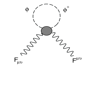
Figure 1: Loop contribution of the operator (3.1), represented by the blob, to the gauge kinetic term.

This contribution has to be cut-off at $M_{s}$, resulting in a value

$$\epsilon_{i}\approx\frac{n_{s}C_{i}}{(4\pi)^{2}}~{},$$ (3.9)

where $n_{s}$ is the number of complex degrees of freedom in $\phi$.

If the scalar $\phi$ has a VEV, both contributions (3.9) and (3.3) are present. In the Standard Model, the higher-dimensional operators that involve the Higgs doublet shift the gauge couplings as in eq. (3.4) with

$$\epsilon_{i}\approx C_{i}\left(\frac{1}{8\pi^{2}}+\frac{v^{2}}{2M_{s}^{2}}\right)~{}.$$ (3.10)

Values for $|\epsilon_{i}|$ of order $10^{-2}$ are quite natural. We emphasize that these corrections to the gauge couplings are present in the Standard Model without the need of any new field beyond the minimal content.

4 Gauge Coupling Unification in Extra Dimensions

The gauge coupling constants in the $\overline{MS}$ scheme at the string scale are related to the measured coupling constants at the $Z$ pole by

$$\overline{\alpha}_{i}^{-1}(M_{s})=\left[\alpha_{i}^{-1}(M_{Z})-\frac{b_{i}}{2\pi}\ln\left(\frac{M_{s}}{M_{Z}}\right)-\frac{\tilde{b}_{i}}{2\pi}{\cal F}(\delta,RM_{s})+\Delta_{i}^{\rm loops}\right]\left(1-4\epsilon_{i}\right)^{-1}~{},$$ (4.1)

where the $(1-4\epsilon_{i})^{-1}$ factor is due to the operators suppressed by powers of $M_{s}$ (see Section 3), ${\cal F}(\delta,R\mu)$ is the one-loop contribution of the KK excitations [see eq. (2.2)]. The $\overline{\alpha}_{i}(\mu)$ represent the coupling constants at the scale $\mu\leq M_{s}$ in the absence of dimension-six or higher operators.

Gauge coupling unification is the condition $\overline{\alpha}_{1}=\overline{\alpha}_{2}=\overline{\alpha}_{3}$ at $M_{s}$. These two equations can be rewritten to leading order in $\epsilon_{i}$ and $\Delta_{i}^{\rm loops}$ as

$$\sum_{i,j,k=1}^{3}\varepsilon^{ijk}\left\{\left(\tilde{b}_{i}-\tilde{b}_{j}\right)\alpha_{0_{k}}^{-1}+4\epsilon_{k}\left[\tilde{b}_{i}\alpha_{0_{j}}^{-1}-\tilde{b}_{j}\alpha_{0_{i}}^{-1}\right]+\left(\tilde{b}_{i}-\tilde{b}_{j}\right)\Delta_{k}^{\rm loops}\right\}={\cal O}\left(\epsilon_{i}^{2},\Delta_{i}^{\rm loops}\right)$$ (4.2)

$${\cal F}(\delta,RM_{s})\approx\frac{2\pi}{\tilde{b}_{3}-\tilde{b}_{1}}\left[\alpha_{0_{3}}^{-1}-\alpha_{0_{1}}^{-1}+\Delta_{3}^{\rm loops}-\Delta_{1}^{\rm loops}+\frac{4(\epsilon_{1}-\epsilon_{3})}{\tilde{b}_{3}-\tilde{b}_{1}}\left(\tilde{b}_{1}\alpha_{0_{3}}^{-1}-\tilde{b}_{3}\alpha_{0_{1}}^{-1}\right)\right]$$ (4.3)

where $\alpha_{0_{i}}^{-1}$ represent the one-loop, inverse coupling constants at $M_{s}$ in the absence of the KK excitations:

$$\alpha_{0_{i}}^{-1}\equiv\alpha_{i}^{-1}(M_{Z})-\frac{b_{i}}{2\pi}\ln\left(\frac{M_{s}}{M_{Z}}\right)~{}.$$ (4.4)

Eq. (4.2) shows that if the sum over $\left(\tilde{b}_{i}-\tilde{b}_{j}\right)\alpha_{0_{k}}^{-1}$ is much smaller than the individual terms in this sum, then the corrections (from two or more loops and from the string dynamics) required by gauge coupling unification are indeed small.

The second unification condition, eq. (4.3), allows us to approximately determine the string scale (assumed to be identical with the unification scale) as a function of the compactification radius and the numbers of extra dimensions, for any model in which the $b_{i}$ and $\tilde{b}_{i}$ coefficients are consistent with eq. (4.3) for small $\Delta_{i}^{\rm loops}$ and $\epsilon_{i}$. In the remainder of this section we analyze these unification conditions in specific models.

4.1 The Standard Model

Consider the Standard Model in Minkowski spacetime plus $\delta$ dimensions of radius $R\sim{\cal O}($TeV${}^{-1})$, with a string scale, $M_{s}$, above but not much larger than $1/R$. In the four-dimensional Standard Model the one-loop $\beta$-function coefficients, above $m_{t}$, are

$$b_{1}=\frac{41}{10}\;,\;\;b_{2}=-\frac{19}{6}\;,\;\;b_{3}=-7\;~{}.$$ (4.5)

To avoid problems with chiral fermions in extra dimensions we assume that the three generations of quarks and leptons are confined in the three-dimensional flat space. Also, we assume that the Higgs doublet cannot propagate in the compact dimensions. This situation can arise due to orbifold compactifications in heterotic string theory, or by duality, due to D-brane configurations in Type I string theory. It can also arise in quantum field theory, if there are domain walls in the $4+\delta$ dimensional theory. In this case the KK excitations contribute at each nondegenerate level to the $\beta$-function coefficients with

$$\tilde{b}_{1}=0\;,\;\;\tilde{b}_{2}=-7\;,\;\;\tilde{b}_{3}=-\frac{21}{2}~{}.$$ (4.6)

We are now in a position to determine how large should be the corrections from the string dynamics to the gauge couplings in order to have gauge coupling unification. Eq.(4.2) gives

$$\epsilon_{3}-1.5\epsilon_{2}+0.6\epsilon_{1}+4.4\times 10^{-3}\left(\Delta_{3}^{\rm loops}-1.5\Delta_{2}^{\rm loops}+0.5\Delta_{1}^{\rm loops}\right)\approx 2.8\times 10^{-2}~{},$$ (4.7)

for $M_{s}\begin{array}[]{c}\,\sim\vspace{-21pt}\\ <\end{array}{\cal O}(10^{2})$ TeV. This shows that indeed the corrections required by gauge coupling unification are small, of order a few percent. As explained in Section 3, values of order $10^{-2}$ for $|\epsilon_{i}|$, as required by the unification condition (4.7), are quite natural.

The other unification condition, eq. (4.3), reads

$${\cal F}(\delta,RM_{s})\approx 25.4\left[1-0.038\ln\left(\frac{M_{s}}{10\;{\rm TeV}}\right)+0.024\left(\Delta_{1}^{\rm loops}-\Delta_{3}^{\rm loops}\right)+5.3\left(\epsilon_{1}-\epsilon_{3}\right)\right]~{}.$$ (4.8)

Using ${\cal F}(\delta,RM_{s})\approx 25$, we compute $RM_{s}$ and the number of KK modes from eq. (2.6) for $\delta=1$, and from eq. (2.3) and Table 1 for $2\leq\delta\leq 6$. The results are presented in Table 2.

$\;\delta\;$	$\;RM_{s}\;$	$\;N_{\rm KK}\;$	$n_{\rm max}$	$N_{c}N_{\rm KK}\alpha_{i}(M_{s})/(4\pi)$
1	$14.8\;$	$28\;$	15	0.12
2	$4.2\;$	$56\;$	11	0.24
3	$2.7\;$	$80\;$	6	0.35
4	$2.2\;$	$88\;$	4	0.38
5	$1.9\;$	$130\;$	3	0.56
6	$1.8\;$	$232\;$	3	1.01

Table 2: The ratio of the string scale to the compactification scale, $RM_{s}$, and the corresponding number of KK modes, $N_{\rm KK}$, and KK levels, $n_{\rm max}$, necessary for gauge coupling unification in the Standard Model, assuming ${\cal F}(\delta,RM_{s})\approx 25$. The loop expansion is reliable for $N_{c}N_{\rm KK}\alpha_{i}(M_{s})\ll 4\pi$.

The phenomenological lower bound on the compactification scale, $R^{-1}\begin{array}[]{c}\,\sim\vspace{-21pt}\\ >\end{array}2.5$ TeV (see the Appendix), can be translated into a lower bound on the string scale: $M_{s}\begin{array}[]{c}\,\sim\vspace{-21pt}\\ >\end{array}40,\,11,\,7,\,5$ TeV for $\delta=1,\,2,\,3,\,\geq 4$, respectively.

From Table 2 one can see that the expansion parameter $N_{c}N_{\rm KK}\alpha_{i}(M_{s})/(4\pi)$ is not much smaller than one, so that perturbation theory is not accurate, especially for more extra dimensions. Only for $\delta=1$, this expansion parameter may be sufficiently small, and it is reasonable to expect corrections of order 10% from two loops. Depending on the values of the different parameters in eq. (4.8), the expansion parameter may be somewhat smaller than the values given in Table 2. For instance, for $M_{s}\approx 40$ TeV, $\epsilon_{2}=-\epsilon_{1}=10^{-2}$, and small $\Delta_{1}^{\rm loops}-\Delta_{2}^{\rm loops}$, one gets ${\cal F}(\delta,RM_{s})\approx 21.4$. For $\delta=1$ this corresponds to $N_{\rm KK}=24$, and an expansion parameter of 0.10.

Nevertheless, we would like to determine more precisely how large the higher order corrections are and how they affect the unification. In the following we will estimate the two-loop RG contributions of the KK states to the running gauge couplings.

A problem of calculating higher loop corrections is that we do not know a gauge invariant regularization method in higher dimensional theories. A truncation of the KK modes at $M_{s}$ (just equivalent to the momentum cutoff in extra dimensions) will not preserve gauge invariance, because the gauge transformation [7]

$$\delta A_{\mu}^{a(n)} = \partial\theta^{a(n)}-{1\over 2}f^{abc}\sum_{m}\left[A_{\mu}^{b(n-m)}+A_{\mu}^{b(n+m)}\right]\theta^{c(m)},$$ (4.9)

$$\delta A_{5}^{a(n)} = -{n\over R}\theta^{a(n)}-{1\over 2}f^{abc}\sum_{m}\left[A_{5}^{b(n-m)}+A_{5}^{b(n+m)}\right]\theta^{c(m)},$$ (4.10)

involves the sum of an infinite number of the KK states. Without knowing a gauge invariant scheme, we will parameterize our ignorance by some unknown parameter in the two-loop calculation.

The two-loop RG equations for the gauge couplings between $R^{-1}$ and $M_{s}$ are

$${d\alpha_{i}^{-1}\over d(\ln\mu)}=-{\tilde{b}_{i}\over 2\pi}N_{\rm KK}(\mu)-{\tilde{b^{\prime}}_{i}\over 2\pi}{\alpha_{i}\over 4\pi}\xi N_{\rm KK}^{2}(\mu),$$ (4.11)

where $N_{\rm KK}(\mu)$ is the number of KK modes below the scale $\mu$, $\tilde{b^{\prime}}_{i}$ are the two-loop RG coefficients for the field content corresponding to one set of KK states, $\tilde{b^{\prime}}_{1}=0$, $\tilde{b^{\prime}}_{2}=-36$, $\tilde{b^{\prime}}_{3}=-81$ [25], and $\xi$ parameterizes our ignorance of a suitable gauge invariant regularization scheme. Naively one would expect $0<\xi<1$ because even if two independent KK state masses (momenta in the extra dimensions) in a two-loop diagram are below $\mu$, the other KK states in the two-loop diagram may have masses greater than $\mu$, hence the corresponding diagram should not be included (at least in a cutoff scheme). For simplicity, we will work in the continuous limit since here we only concern about the relative sizes of the one-loop and two-loop contributions. In this limit, $N_{\rm KK}(\mu)\approx(R\mu)^{\delta}\pi^{\delta/2}/\Gamma(1+\delta/2)$ is the volume of a $\delta$-dimensional sphere of radius $R\mu$.

For a given compactification scale $R^{-1}$ we can solve (4.11) numerically with the initial value $\alpha_{i}^{-1}(R^{-1})$ obtained from the usual 4-dimensional running below $1/R$ (where one loop is sufficient). The results are shown in Fig. 2 for $R^{-1}=3$ TeV, $\delta=1,\,2$, and $\xi=0$ (one-loop running) and $\xi=1$.

                 

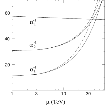
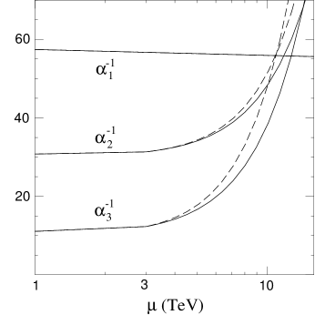
a                                                                  b

Figure 2: Running of the SM gauge couplings for a) $\delta=1$, and b) $\delta=2$ extra dimensions. Solid curves are the 1-loop results in the continuous limit. The dashed curves include the two-loop contributions from the KK states, assuming $\xi=1$ in Eq. (4.11). The KK excitations of the gauge bosons do not affect $\alpha_{1}^{-1}$ directly because the gauge group is Abelian. The compactification scale is assumed to be $1/R=3$ TeV.

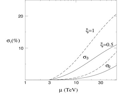
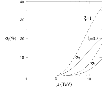
a                                                                  b

Figure 3: The percentage corrections of $\alpha_{2}^{-1}$ and $\alpha_{3}^{-1}$in the Standard Model due to the 2-loop effects, $\sigma_{i}=(\alpha_{i,\,{\rm 2-loop}}^{-1}/\alpha_{i,\,{\rm 1-loop}}^{-1})(\mu)-1$, with $\xi=0.5$ (solid lines) and $\xi=1$ (dashed lines), for: a) $\delta=1$, and b) $\delta=2$.

We can see that the two-loop contributions improve the unification for typical values of the unknown $\xi$ factor. Of course, this is sensible only if the perturbation series converge and higher loop effects are small. In Fig. 3 we plot the percentages of corrections due to the two-loop effects.

For $\delta=1$ and $\xi=1$, the corrections are $\sim 15\%$ for $\alpha_{3}^{-1}$ and $\sim 5\%$ for $\alpha_{2}^{-1}$. The corrections are roughly proportional to $\delta$ and $\xi$. It suggests that the perturbation series probably still holds for small number of extra dimensions and may break down for more extra dimensions. Note that the two-loop contributions reduce the gauge couplings as well as the unification scale, so the expansion parameters $\propto N_{\rm KK}\alpha_{i}$ are smaller than the one-loop estimate (assuming that $\xi>0$). Given possible corrections from string scale effects (discussed in Section 3) and from higher loops, the Standard Model gauge couplings are consistent with unification at the string scale without the need of introducing new fields to change the $\beta$-functions [26], at least for small number of extra dimensions where the perturbation series can still be trusted.

4.2 Higgs Compositeness from Extra Dimensions

The condition of gauge coupling unification at one loop leads to the conclusion that the gauge theory is in, or close to the non-perturbative regime if there are more than one extra dimensions, as can be seen by inspecting the values of the expansion parameter $N_{c}N_{\rm KK}\alpha_{i}(M_{s})/(4\pi)$ in Table 2. The reason for that is that the higher-dimensional gauge coupling is dimensionful such that the strength of the gauge interactions increases rapidly above $R^{-1}$ [27].

One possible effect of the non-perturbativity at the string scale is the dynamical breaking of the chiral symmetry [18]. If this is the case, then the fundamental Higgs doublet from the Standard Model may be replaced with a composite Higgs, made up of the left-handed top-bottom doublet and the right-handed component of a heavy vector-like quark [28].

The running of the gauge couplings in this case is almost the same as in the Standard Model, assuming as in Section 4.1 that all the fermions are confined on 3-branes. The one-loop $\beta$-function coefficients due to a nondegenerate set of KK excitations is given by eq. (4.6).

The one-loop $\beta$-function coefficients due to zero modes are slightly different than in the Standard Model. First, there is need for a vector-like quark, $\chi$, with the same charges as the right-handed top. Its mass $m_{\chi}$ is in the TeV range, so that the logarithmic running due to this vector-like quark, between $m_{\chi}$ and $M_{s}$, is negligible. In addition to a composite Higgs doublet, other quark-antiquark bound states may form, depending on the flavor structure of the four-quark operators induced at the string scale [18], and on the position of the fermions in the extra dimensions [11]. These composite scalars do not have KK modes, and contribute logarithmically to the gauge coupling running between their masses and $R^{-1}$ (the compositeness scale is roughly given by the compactification scale). This ensures gauge coupling unification with a precision comparable with the one in the Standard Model in extra dimensions.

Given that electroweak symmetry breaking occurs only for more than one extra dimensions, where the dynamics of the gluonic KK modes is strongly coupled, it is not possible to predict reliably that gauge couplings unify in this scenario. However, it is interesting that, due to the presence of the extra dimensions, gauge coupling unification is compatible with the formation of a composite Higgs doublet.

4.3 Minimal Supersymmetric Standard Model

We now turn to supersymmetric models in extra dimensions. Supersymmetric operators induced at the string scale give corrections to the gauge couplings of the order of the $SU(3)_{C}\times SU(2)_{W}\times U(1)_{Y}$ invariant holomorphic combinations of VEVs suppressed by the appropriate power of $M_{s}$. As mentioned in Section 3, in the MSSM these corrections are likely to be below 1%, while in the NMSSM they may be as large as 10%.

In the four-dimensional MSSM the one-loop $\beta$-function coefficients above the superpartner masses are given by

$$b_{1}=\frac{33}{5}\;,\;\;b_{2}=1\;,\;\;b_{3}=-3\;~{}.$$ (4.12)

Assuming as in Ref. [7] that only the vector multiplets and the two Higgs supermultiplets propagate in the compact dimensions, the KK excitations give

$$\tilde{b}_{1}=\frac{3}{5}\;,\;\;\tilde{b}_{2}=-3\;,\;\;\tilde{b}_{3}=-6~{}.$$ (4.13)

The unification conditions (4.2) and (4.3) are given in the MSSM by

$$\epsilon_{3}-1.8\epsilon_{2}+0.05\epsilon_{1}+5.0\times 10^{-3}\left(\Delta_{3}^{\rm loops}-1.8\Delta_{2}^{\rm loops}+0.83\Delta_{1}^{\rm loops}\right)\approx-1.4\times 10^{-2}~{},$$ (4.14)

$${\cal F}(\delta,RM_{s})\approx 41.3\left[1-0.035\ln\left(\frac{M_{s}}{10\;{\rm TeV}}\right)+0.023\left(\Delta_{1}^{\rm loops}-\Delta_{3}^{\rm loops}\right)+4.6\left(\epsilon_{1}-\epsilon_{3}\right)\right]~{}.$$ (4.15)

for $M_{s}\begin{array}[]{c}\,\sim\vspace{-21pt}\\ <\end{array}{\cal O}(10^{2})$ TeV. The first equation here shows that the corrections required by gauge coupling unification are again of order a few percent, and slightly smaller than in the Standard Model. In Section 3 we argued that the $\epsilon_{i}$ are below one percent in the MSSM [see eq. (3.6)], and could be as large as 10% in the NMSSM.

Eq. (4.15) shows that ${\cal F}(\delta,RM_{s})$, and consequently the number of KK modes required by gauge coupling unification, is larger than in the Standard Model. This is due to the fact that the coefficients of the one-loop $\beta$-functions are smaller in the MSSM. The number of KK modes, $N_{\rm KK}$, and the loop expansion parameter $N_{c}N_{\rm KK}\alpha_{i}(M_{s})/(4\pi)$ are listed in Table 3. The expansion parameter appears to be too large (with the possible exception of $\delta=1$) to allow a reasonable convergence of the perturbative series.

The KK excitations of the MSSM fields form complete ${\cal N}=2$ supersymmetric multiplets [7, 29, 30]. Since there is no wave function renormalization beyond one-loop in ${\cal N}=2$ supersymmetric theories, it has been argued that it is legitimate to study gauge coupling unification by keeping only the one-loop running of the gauge couplings. In fact there are higher-loop contributions to the gauge couplings from Feynman diagrams involving at least one zero-mode [29]. These are subleading order in the large $N_{\rm KK}$ limit, so that the one-loop contribution is indeed the largest one. However, this does not improve the convergence of the perturbative expansion, because all the terms in this series are of the same order (albeit smaller than the one-loop term) for $\delta\begin{array}[]{c}\,\sim\vspace{-21pt}\\ >\end{array}2$. Therefore, we conclude based on the entries in last column of Table 3 that the corrections to the gauge couplings in the MSSM are large, and if there is gauge coupling unification in the presence of more than one compact dimension, then this happens in the non-perturbative regime.

$\;\delta\;$	$\;RM_{s}\;$	$\;N_{\rm KK}\;$	$n_{\rm max}$	$N_{c}N_{\rm KK}\alpha_{i}(M_{s})/(4\pi)$
1	$22.5\;$	$44\;$	22	0.22
2	$5.2\;$	$88\;$	14	0.44
3	$3.1\;$	$122\;$	8	0.60
4	$2.4\;$	$136\;$	5	0.68
5	$2.1\;$	$220\;$	4	1.1
6	$1.9\;$	$232\;$	3	1.2

Table 3: The ratio of the string scale to the compactification scale, $RM_{s}$, and the number of KK modes, $N_{\rm KK}$, and KK levels, $n_{\rm max}$, required by gauge coupling unification in the MSSM, for ${\cal F}(\delta,RM_{s})\approx 40$. The loop expansion works well for $N_{c}N_{\rm KK}\alpha_{i}(M_{s})\ll 4\pi$.

Finally, we note that the gauge invariant operators that are expected to be induced by the string dynamics have an impact on four-dimensional supersymmetric models too. If all these operators are generated with coefficients of order one times the appropriate power of $M_{s}$, then any model that reduces to the MSSM at low energy should include new gauge symmetries that forbid the dangerous effects, such as proton decay, FCNC’s, a large $\mu$ term, and so on. The models of this type [31] do not accommodate gauge coupling unification in any obvious way.

5 Conclusions

Our present analysis suggests the following conjecture: theories in which there are new dimensions at the $\sim$ TeV scale are strongly coupled theories in the gauge couplings of $SU(3)_{C}\times SU(2)_{W}\times U(1)_{Y}$. This has two important implications. First, electroweak symmetry breaking may be induce by this strong dynamics. Much effort must now go into understanding strongly coupled theories in extra-dimensions, and we defer this to future studies.

The second implication, considered in the present paper, is that potentially large uncertainties may affect gauge coupling unification. We have shown (as an example, rather than a serious model proposal) that even the minimal Standard Model is consistent with unification in the presence of compact dimensions and higher-dimensional operators that are expected to be induced by the string dynamics. Of course, unification is occurring at or near the string scale where the precise physical meaning of unification is less clear.

The coefficients of the new higher dimensional operators cannot be computed without a complete knowledge of and computational capability within the string theory. Given these uncertainties we argue that the gauge coupling unification is not a strong constraint on a large class of models.

Acknowledgements: We would like to thank Joe Lykken, Konstantin Matchev, Stuart Raby, and Eric Weinberg for useful discussions.

Appendix:  Lower Bounds on the Compactification and String Scales

In this Appendix we discuss the lower bounds on the compactification scale for the extra dimensions where Standard Model gauge fields propagate, and the string scale.

There are various experimental bounds on the compactification scale. Direct searches for heavy gauge bosons put limits on the masses of the KK states of the Standard Model gauge bosons. It is useful to observe that the KK modes of the gluons have the same couplings (up to an overall normalization) and properties as the flavor-universal colorons [32]. By searching for new particles decaying to two-jets, CDF gives a lower limit of 980 GeV on the flavor-universal colorons [33], and D0 put lower limits on additional Standard Model $W$ and $Z$ bosons of 680 GeV and 615 GeV respectively [34]. Therefore, the compactification scale $R^{-1}$ has to be greater than about 1 TeV.

There are also indirect limits from the electroweak observables and higher dimensional operators (e.g., four fermion operators) generated from integrating out the heavy KK gauge bosons [13, 35, 36, 37, 38]. Many of them are related to the Fermi constant $G_{F}$, since it is very precisely measured and is used as an input parameter for determining other observables. For example, in Ref. [35], it was claimed that from the precision determination of $G_{F}$, one can exclude the compactification scale below $\sim$ 1.6 TeV, 3.5 TeV, 5.7 TeV, and 7.8 TeV for 1, 2, 3, and 4 extra dimensions. However, these indirect constraints are not as robust as the constraints from direct searches, since there may be some other unknown contributions to these observables. As we have seen in the previous section, the string scale $M_{s}$ is expected to be not far above the compactification scale, due to the rapid convergence of the gauge couplings (and also the rapid growing of the ’t Hooft coupling $N_{\rm KK}g^{2}$) above the compactification scale. In that case, we expect that there are higher dimensional operators, generated from the string scale physics, including those with the same form as the ones induced by the exchange of KK modes. They are suppressed by a somewhat larger string scale mass, but they do not have the small gauge coupling suppression as those coming from integrating out KK gauge bosons. As a result, their sizes could be comparable and they could cancel each other.

In addition, the corrections from integrating out KK modes for some observables also depend on how the four-dimensional theory is embedded into higher dimensions. For example, the corrections to $G_{F}$ can be of opposite signs depending on whether the Higgs propagates in the bulk or only on the wall [36], and whether the muon and the electron are localized at the same point in the extra dimensions [11]. If different fermion species in a higher dimensional operator are localized at different points in the compact dimensions, the KK states will have different couplings to these fermions and the sum of the contributions of all KK states may not add up. This can give the right-sign correction to the atomic parity violation [11]. The strongest bound comes from the leptonic width of the $Z$, $\Gamma(l^{+}l^{-})$, which gives $R^{-1}\begin{array}[]{c}\,\sim\vspace{-21pt}\\ >\end{array}2.5$ TeV for one extra dimension [36]. However, as we discussed above, this bound is still model dependent and may be lowered by different arrangements of the Higgs and leptons in the extra dimensions (e.g., in the bulk or on the wall, same point or different points, etc.) and extra contributions to the electroweak parameters from the string dynamics.

Now we turn to bounds on the string scale, $M_{s}$. In addition to the effect of producing gauge dielectric constants, discussed in Section 3, the operators associated with a low string scale and the extra dimensions at a TeV scale may have many new implications for physics at lower energies. Some of these operators have been analyzed in Ref. [12].

The fundamental theory incorporates quantum gravity, so that it is expected that string scale physics will generate higher dimensional gauge invariant operators at $M_{s}$. If all such higher dimensional operators suppressed by the appropriate powers of the fundamental scale, $M_{s}$, are generated with coefficients of order one, then the strong constraints from proton decay, flavor changing processes, and CP violation will push $M_{s}$ to a very high scale, reintroducing the hierarchy problem. However, these problems are closely related to the pattern of flavor symmetry breaking. They may have some higher dimensional solutions [7, 11], or can be avoided if there is a large flavor symmetry [27, 12]. For flavor-conserving operators, the constraints coming from compositeness searches on the four fermion operators require that $M_{s}\begin{array}[]{c}\,\sim\vspace{-21pt}\\ >\end{array}1$ TeV [21, 39]. The strongest constraints come from the precision measurements of the electroweak sector [12, 40, 41]. The operators

$${\cal O}_{BW} = {c_{BW}\over M_{s}^{2}}B^{\mu\nu}\left(H^{\dagger}{\sigma^{a}\over 2}W^{a}_{\mu\nu}H\right),$$ (A.1)

$${\cal O}_{H} = {c_{H}\over M_{s}^{2}}\left(H^{\dagger}{\cal D}^{\mu}H\right)\left({\cal D}_{\mu}H^{\dagger}H\right),$$ (A.2)

contribute to the $S$ and $T$ parameters respectively [42, 12]. A global fit to the electroweak observables gives the constraints [12]

$${M_{s}\over\sqrt{c_{BW}}} > 3.6\;\rm{TeV},$$ (A.3)

$${M_{s}\over\sqrt{c_{H}}} > 3.0\;\rm{TeV}~{}.$$ (A.4)

Note that these constraints apply at the electroweak scale while the higher dimensional operators are generated at the string scale. In running from the string scale down to the electroweak scale, the coefficients of these operators are renormalized not only by themselves but also form the operators (3.1). Although they receive power law corrections between the string scale and the compactification scale, we do not expect more than a factor of 2 modifications due to the smallness of $g_{1}$ and $g_{2}$, and closeness between the two scales (for comparison, $\alpha_{2}$ changes by a factor of about 2.) The one loop contributions of the operators (3.1) to (A.1) and hence to $S$ were calculated in Ref. [42]. They are roughly of the order $0.1\times(c_{WW},\,c_{BB})$, so the direct constraints on the operators (3.1) from $S$ and $T$ are not very strong. There are also various higher dimensional operators which give non-universal contributions to individual observables. The constraints depend sensitively on the sizes and signs of the coefficients of these operators. Assuming that all coefficients are $\pm 1$ [41], $M_{s}\sim 5$ TeV is still allowed for some choices of the signs.

References

- [1] H. Georgi and S. L. Glashow, Phys. Rev. Lett. 32 (1974) 438.
-
[2]
J. Ellis, S. Kelley and D.V. Nanopoulos,
Phys. Lett. B249 (1990) 441; Phys. Lett. B260 (1991) 131;
P. Langacker and M. Luo, Phys. Rev. D44 (1991) 817;
U. Amaldi, W. de Boer and H. Furstenau, Phys. Lett. B260 (1991) 447;
C. Giunti, C.W. Kim and U.W. Lee, Mod. Phys. Lett. A6 (1991) 1745;
M. Carena, S. Pokorski and C.E. Wagner, Nucl. Phys. B406 (1993) 59, hep-ph/9303202. -
[3]
J. Bagger, K. Matchev and D. Pierce,
Phys. Lett. B348, 443 (1995), hep-ph/9501277;
P. Langacker and N. Polonsky, Phys. Rev. D52, 3081 (1995), hep-ph/9503214;
D.M. Pierce, J.A. Bagger, K. Matchev and R. Zhang, Nucl. Phys. B491, 3 (1997), hep-ph/9606211. - [4] C. Caso, et al, Euro. Phys. Journal C3 (1998) 1.
- [5] L. Hall, Nucl. Phys. B178, 75 (1981).
-
[6]
C. T. Hill, Phys. Lett. B135 47(1984);
Q. Shafi and C. Wetterich, Phys. Rev. Lett. 52 (1984) 875. - [7] K. R. Dienes, E. Dudas, and T. Ghergheta, Phys. Lett. B436, 55 (1998), hep-ph/9803466; Nucl. Phys. B537, 47 (1999), hep-ph/9806292.
- [8] I. Antoniadis, Phys. Lett. B246 (1990) 377.
-
[9]
D. Ghilencea and G. G. Ross, Phys. Lett. B442, 165 (1998),
hep-ph/9809217;
S. A. Abel and S. F. King, Phys. Rev. D59, 095010 (1999), hep-ph/9809467;
C. D. Carone, hep-ph/9902407;
A. Delgado and M Quiros, hep-ph/9903400. - [10] A. Perez-Lorenzana and R.N. Mohapatra, hep-ph/9904504.
- [11] N. Arkani-Hamed and M. Schmaltz, SLAC-PUB-8082, hep-ph/9903417.
- [12] L. Hall and C. Kolda, LBNL-43085, hep-ph/9904236.
-
[13]
T. Rizzo and J. Wells, hep-ph/9905234;
A. Strumia, hep-ph/9906266. -
[14]
M. Dine and N. Seiberg, Phys. Lett. B162 (1985) 299;
M. Dine, hep-ph/9905219. - [15] J. Lykken, Phys. Rev. D54, 3693 (1996), hep-th/9603133.
-
[16]
N. Arkani-Hamed, S. Dimopoulos and G. Dvali,
Phys. Lett. B429, 263 (1998), hep-ph/9803315;
I. Antoniadis, N. Arkani-Hamed, S. Dimopoulos and G. Dvali, Phys. Lett. B436 (1998) 257. hep-ph/9804398. - [17] L. Randall and R. Sundrum, MIT-CTP-2860, hep-ph/9905221.
- [18] B. A. Dobrescu, hep-ph/9812349 and hep-ph/9903407.
- [19] For a review, see K. R. Dienes, Phys. Reports 287 (1997) 447, hep-th/9602045.
- [20] G. Shiu and S.-H. H. Tye, Phys. Rev. D58, 106007 (1998), hep-th/9805157.
- [21] N. Arkani-Hamed, S. Dimopoulos and G. Dvali, Phys. Rev. D59, 086004 (1999), hep-ph/9807344.
-
[22]
Z. Kakushadze and S.-H. H. Tye, hep-th/9809147;
C. P. Bachas, hep-ph/9807415;
L. E. Ibanez, hep-ph/9905349;
I. Antoniadis, C. Bachas, and E. Dudas, hep-th/9906039. - [23] L.J. Hall and U. Sarid, Phys. Rev. Lett. 70 (1993) 2673, hep-ph/9210240.
- [24] E. Witten, Nucl. Phys. B258 (1985) 75.
- [25] M.E. Machacek and M.T. Vaughn, Nucl. Phys. B222, 83 (1983).
- [26] P. H. Frampton and A. Rasin, IFP-769-UNC, hep-ph/9903479.
- [27] N. Arkani-Hamed and S. Dimopoulos, SLAC-PUB-8008, hep-ph/9811353.
-
[28]
B. A. Dobrescu and C. T. Hill, Phys. Rev. Lett. 81 (1998) 2634,
hep-ph/9712319;
R. S. Chivukula, B. A. Dobrescu, H. Georgi, and C. T. Hill, Phys. Rev. D59 (1999) 075003, hep-ph/9809470. -
[29]
Z. Kakushadze, HUTP-98-A073, hep-th/9811193 ;
Z. Kakushadze and T. R. Taylor, HUTP-99-A019, hep-th/9905137. - [30] K. R. Dienes, E. Dudas and T. Gherghetta, hep-ph/9807522.
- [31] H.-C. Cheng, B. A. Dobrescu, and K. T. Matchev, Nucl. Phys. B543 47, (1999), hep-ph/9811316.
-
[32]
R.S. Chivukula, A.G. Cohen and E.H. Simmons,
Phys. Lett. B380 (1996) 92,
hep-ph/9603311;
E.H. Simmons, Phys. Rev. D55 (1997) 1678, hep-ph/9608269;
M.B. Popovic and E.H. Simmons, Phys. Rev. D58 (1998) 095007, hep-ph/9806287;
I. Bertram and E. H. Simmons, Phys. Lett. B443 (1998) 347, hep-ph/9809472. - [33] F. Abe, et al. (CDF Collaboration), Phys. Rev. D55, 5263 (1997), hep-ex/9702004.
- [34] B. Abbott et al. (D0 Collaboration), XVIII International Symposium on Lepton-Photon Interactions, Hamburg, Germany, July 18-August 1, 1997, Fermilab-Conf-97/356-E.
- [35] P. Nath and M. Yamaguchi, hep-ph/9902323 and hep-ph/9903298.
- [36] M. Masip and A. Pomarol, CERN-TH/99-47, hep-ph/9902467.
- [37] W. J. Marciano, hep-ph/9902332 and hep-ph/9903451.
- [38] I. Antoniadis, K. Benakli and M. Quirós, CERN-TH/99-128, hep-ph/9905311.
- [39] K. Cheung, UCD-HEP-99-10, hep-ph/9904510.
- [40] T. Banks, M. Dine, and A. E. Nelson, SCIPP-99/03, hep-th/9903019.
- [41] R. Barbieri and A. Strumia, IFUP-TH/21-99, hep-ph/9905281.
-
[42]
K. Hagiwara, S. Ishihara, R. Szalapski and
D. Zeppenfeld, Phys. Rev. D48, 2182 (1993);
K. Hagiwara, T. Hatsukano, S. Ishihara and R. Szalapski, Nucl. Phys. B496 (1997) 66, hep-ph/9612268.