Abstract

The interaction potential $V(Q^{2})$ between static test charges can be used to define an effective charge $\alpha_{V}(Q^{2})$ and a physically-based renormalization scheme for quantum chromodynamics and other gauge theories. In this paper we use recent results for the finite-mass fermionic corrections to the heavy-quark potential at two-loops to derive the next-to-leading order term for the Gell Mann-Low function of the $V$-scheme. The resulting effective number of flavors $N_{F}(Q^{2}/m^{2})$ in the $\alpha_{V}$ scheme is determined as a gauge-independent and analytic function of the ratio of the momentum transfer to the quark pole mass. The results give automatic decoupling of heavy quarks and are independent of the renormalization procedure. Commensurate scale relations then provide the next-to-leading order connection between all perturbatively calculable observables to the analytic and gauge-invariant $\alpha_{V}$ scheme without any scale ambiguity and a well defined number of active flavors. The inclusion of the finite quark mass effects in the running of the coupling is compared with the standard treatment of finite quark mass effects in the $\overline{\mbox{MS}}$ scheme.

I Introduction

Is there a preferred effective charge which should be used to characterize the coupling strength in QCD? In principle, any perturbatively calculable observable can be used to define an effective charge. In quantum electrodynamics, the Dyson running coupling $\alpha_{\mbox{QED}}(Q^{2})$, defined from the linearized potential between two infinitely-heavy test charges, has been used as the traditional coupling. The corresponding definition of the non-abelian QCD coupling is customarily given by identifying the ground state energy of the vacuum expectation value of the Wilson loop as the potential $V$ between a static quark-antiquark pair in a color singlet state [1]:

$$V(r,m^{2})=-\lim_{t\rightarrow\infty}\frac{1}{it}\log\langle 0|Tr\;\left\{P\;\exp\left(\oint dx_{\mu}A^{\mu}_{a}T^{a}\right)\right\}|0\rangle$$ (1)

where $r$ denotes the relative distance between the heavy quarks, $m$ is the mass of “light” quarks contributing through loop effects, and $T^{a}$ are the generators of the gauge group. It is then convenient to define the effective charge $\alpha_{V}(Q^{2},m^{2})$ as

$$V(Q^{2},m^{2})\equiv-4\pi C_{F}\frac{\alpha_{V}(Q^{2},m^{2})}{{Q}^{2}}$$ (2)

in momentum space. The factor $C_{F}$ is the value of the Casimir operator $T^{a}T^{a}$ of the external sources (which are in the fundamental representation) and factors out to all orders in perturbation theory, and $Q^{2}=-q^{2}$ is the spacelike momentum transfer.

The effective charge $\alpha_{V}(Q)$ provides a physically-based alternative to the usual modified minimal subtraction ($\overline{\mbox{MS}}$) scheme. As in the corresponding case of Abelian QED, the scale $Q$ of the coupling $\alpha_{V}(Q)$ is given by the exchanged momentum. There is thus no ambiguity in the interpretation of the scale. All virtual corrections due to massive fermion pairs are incorporated in $\alpha_{V}$ through loop diagrams which depend on the physical mass thresholds. When continued to time-like momenta, the coupling has the correct analytic dependence dictated by the production thresholds in the crossed channel. Since $\alpha_{V}$ incorporates quark mass effects exactly, it avoids the problem of explicitly computing and resumming quark mass corrections which are related to the running of the coupling. Thus the effective number of flavors $N_{F}(Q/m)$ is an analytic function of the scale $Q$ and the quark masses $m$. The effects of finite quark mass corrections on the running of the strong coupling were first considered by De Rújula and Georgi [2] within the momentum subtraction schemes (MOM) (see also [3, 4, 5, 6]). The two-loop calculation was first done by Yoshino and Hagiwara [7] in the MOM-scheme using Landau gauge and also recently by Jegerlehner and Tarasov [8] using background field gauge.

One important advantage of the physical charge approach is its inherent gauge invariance to all orders in perturbation theory. This feature is not manifest in massive $\beta$-functions defined in non-physical schemes such as the MOM schemes. A second, more practical, advantage is the automatic decoupling of heavy quarks according to the Appelquist-Carazzone theorem [9].

By employing the commensurate scale relations [10] other physical observables can be expressed in terms of the analytic coupling $\alpha_{V}$ without scale or scheme ambiguity. The quark mass threshold effects in the running of the coupling are taken into account by utilizing the mass dependence of the physical $\alpha_{V}$ scheme. In effect, quark thresholds are treated analytically to all orders in $m^{2}/Q^{2}$; i.e., the evolution of the physical $\alpha_{V}$ coupling in the intermediate regions reflects the actual mass dependence of a physical effective charge and the analytic properties of particle production. Furthermore, the definiteness of the dependence in the quark masses automatically constrains the scale $Q$ in the argument of the coupling. There is thus no scale ambiguity in perturbative expansions in $\alpha_{V}$.

In the conventional $\overline{\mbox{MS}}$ scheme, the coupling is independent of the quark masses since the quarks are treated as either massless or infinitely heavy with respect to the running of the coupling. Thus one formulates different effective theories depending on the effective number of quarks which is governed by the scale $Q$; the massless $\beta$-function is used to describe the running in between the flavor thresholds. These different theories are then matched to each other by imposing matching conditions at the scale (normally the quark masses) where the effective number of flavors is changed. The dependence on the matching scale can be made arbitrarily small by calculating the matching conditions to high enough order. For physical observables one can then include the effects of finite quark masses by making a higher-twist expansion in $m^{2}/Q^{2}$ and $Q^{2}/m^{2}$ for light and heavy quarks, respectively. These higher-twist contributions have to be calculated for each observable separately, so that in principle one requires an all-order resummation of the mass corrections to the effective Lagrangian to give correct results.

The specification of the coupling and renormalization scheme also depends on the definition of the quark mass. In contrast to QED where the on-shell mass provides a natural definition of lepton masses, an on-shell definition for quark masses is complicated by the confinement property of QCD. In this paper we will use the pole mass $m$ which has the advantage of being scheme and renormalization-scale invariant.

A technical complication of massive schemes is that one cannot easily obtain analytic solutions of renormalization group equations to the massive $\beta$ function, and the Gell-Mann Low function is scheme-dependent even at lowest order.

In this paper we present a two-loop analytic extension of the $\alpha_{V}$-scheme based on the recent results of Ref. [11]. The mass effects are in principle treated exactly to two-loop order and are only limited in practice by the uncertainties from numerical integration. The desired features of gauge invariance and decoupling are manifest in the form of the two-loop Gell-Mann Low function, and we give a simple fitting-function which interpolates smoothly the exact two-loop results obtained by using the adoptive Monte Carlo integrator VEGAS[12]. Strong consistency checks of the results are performed by comparing the Abelian limit to the well known QED results in the on-shell scheme. In addition, the massless as well as the decoupling limit are reproduced exactly, and the two-loop Gell-Mann Low function is shown to be renormalization scale ($\mu$) independent.

As an application we show how the analytic $\alpha_{V}$-scheme can be used to calculate the non-singlet hadronic width of the Z-boson, including finite quark mass corrections from the running of the coupling and compare with the standard treatment in the $\overline{\mbox{MS}}$ scheme where the corresponding effects are calculated as higher twist corrections.

Recently (see Ref. [13]) we proposed an alternative way of incorporating mass effects connected with the running of the coupling by making an analytic extension of the $\overline{\mbox{MS}}$-scheme where the coupling is an analytic function of both the scale and the quark masses. This analytic extension of the $\overline{\mbox{MS}}$-scheme is defined by connecting the $\overline{\mbox{MS}}$ coupling to the $V$-scheme using a commensurate scale relation based on the (BLM) scale-setting procedure[14]. The new modified coupling $\widetilde{\alpha}_{\overline{\mbox{MS}}}(Q)$ inherits most of the good properties of the $\alpha_{V}$ scheme, including its correct analytic properties as a function of the quark masses and its unambiguous scale fixing [13].

However, the conformal coefficients in the commensurate scale relation between the $\alpha_{V}$ and $\overline{\mbox{MS}}$ schemes do not preserve one of the defining criterion of the potential expressed in the bare charge, namely the non-occurrence of color factors corresponding to an iteration of the potential. This is probably an effect of the breaking of conformal invariance by the $\overline{\mbox{MS}}$ scheme. The breaking of conformal symmetry has also been observed when dimensional regularization is used as a factorization scheme in both exclusive [15, 16] and inclusive [17] reactions. Thus, it does not turn out to be possible to extend the modified scheme ${\widetilde{\alpha}}_{\overline{\mbox{MS}}}$ beyond leading order without running into an intrinsic contradiction with conformal symmetry. Note, however, that this difficulty does not affect using the $\overline{\mbox{MS}}$ scheme as an intermediate renormalization scheme when connecting physical observables. For completeness we give the results of such an extension in an appendix.

The paper is organized as follows: In section II we derive the second term of the Gell-Mann Low function in the physical $V$-scheme as a renormalization-scale-independent function of the ratio of the physical momentum transfer $Q$ and the pole mass $m$. In section III we present numerical results of the effective number of flavors and compare it with results obtained in the gauge-dependent momentum subtraction schemes. In addition, various consistency checks are performed, and numerical fits are presented. In section IV we illustrate some of the properties of the analytic $\alpha_{V}$ scheme and demonstrate the effect of the quark mass thresholds on the mass-dependent evolution and compare with the massless evolution. In section V we compare the calculation of the hadronic width of the $Z$-boson in the analytic $\alpha_{V}$ scheme to the conventional $\overline{\mbox{MS}}$ scheme with a mass-independent coupling and explicit higher-twist corrections for mass effects. In section VI we summarize our results and indicate future applications. The definition of the analytically extended scheme ${\widetilde{\alpha}}_{\overline{\mbox{MS}}}$ beyond leading order is discussed in the appendix.

II The Gell-Mann Low Function Through Two Loops

The physical charge $\alpha_{V}(Q,m)$ can be expressed as a perturbative series in any other renormalization scheme. For example, in the minimal subtraction scheme, the perturbative series has the form:

$$\alpha_{V}(Q,m) = \alpha_{{\mbox{MS}}}(\mu)\left(1+v_{1}(Q,m(\mu),\mu)\frac{\alpha_{{\mbox{MS}}}(\mu)}{\pi}+v_{2}(Q,m(\mu),\mu)\frac{\alpha^{2}_{{\mbox{MS}}}(\mu)}{\pi^{2}}+\cdots\right)$$ (3)

where the massless limit of the coefficients $v_{1}$ and $v_{2}$ are known in the literature [1, 18, 19, 20, 21, 22, 23]. Since the physical charge $\alpha_{V}(Q,m)$ cannot depend on the renormalization scale $\mu$, the $\mu$-dependence on the right-hand side of Eq. (3) must cancel to the order we are working. Notice that the coefficients also depend on the renormalization scale $\mu$ used for the mass renormalization, i.e. through the dependence of the running mass $m(\mu)$. Fig. 1 shows the Feynman diagrams for the fermionic contributions to the two-loop coefficient $v_{2}(Q,m(\mu),\mu)$. These contributions depend on the mass renormalization used for the one-loop coefficient $v_{1}(Q,m(\mu),\mu)$. Since we are predominantly interested in the flavor-threshold dependence of heavy quarks, we shall relate the running mass to the pole mass which is renormalization-scale independent and gives explicit decoupling. This also provides a physical picture as well as a straightforward Abelian limit.

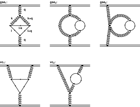
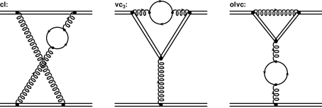
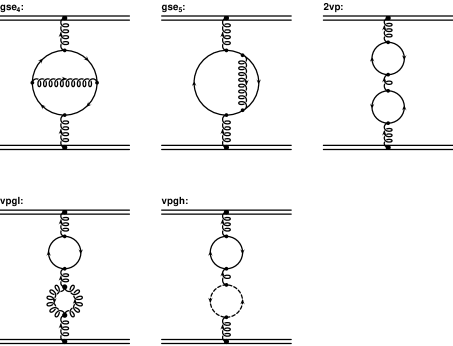
FIG. 1.: The two-loop massive fermionic corrections to the heavy quark potential (from [11]). Double lines denote the heavy quarks, single lines the “light” quarks with mass $m$. The first two rows contain diagrams with a typical non-Abelian topology. The middle line includes the infrared divergent “Abelian” Feynman diagrams. They contribute to the potential only in the non-Abelian theory due to color factors $\propto C_{F}C_{A}$. In addition, although each diagram is infrared divergent, their sum is infrared finite. The infrared finite Feynman diagrams with an Abelian topology plus the diagrams consisting of one-loop insertions with non-Abelian terms are shown in the last two rows.

The next-to-leading order relation between the MS mass $m(\mu)$ and the pole mass $m$ is given by [24],

$$m(\mu)=m\left[1-C_{F}\frac{\alpha_{{\mbox{MS}}}(\mu)}{\pi}\left(1+\frac{3}{2}\log\frac{\mu}{m}-\frac{3}{4}\left[\gamma-\log(4\pi)\right]\right)\right],$$ (4)

where $\gamma$ is the Euler constant. Inserting Eq. (4) into Eq. (3) gives at next-to-next-to-leading order

$$\alpha_{V}(Q,m) = \alpha_{{\mbox{MS}}}(\mu)\left[1+v_{1}(Q,m,\mu)\frac{\alpha_{{\mbox{MS}}}(\mu)}{\pi}+\left[v_{2}(Q,m,\mu)+\Delta_{m}(Q,m,\mu)\right]\frac{\alpha_{\mbox{MS}}^{2}(\mu)}{\pi^{2}}\right]$$ (5)

where $\Delta_{m}(Q,m,\mu)$ denotes the contribution arising from $v_{1}$ when changing from the MS mass to the pole mass: $v_{1}(Q,m(\mu),\mu)=v_{1}(Q,m,\mu)+\Delta_{m}(Q,m,\mu)\frac{\alpha_{{\mbox{MS}}}(\mu)}{\pi}.$

The Gell-Mann Low function [25] for the $V$-scheme is defined as the total logarithmic derivative of the effective charge with respect to the physical momentum transfer scale $Q$:

$$\Psi_{V}\left(\frac{Q}{m}\right)\equiv\frac{d\alpha_{V}(Q,m)}{d\log Q}\equiv\sum^{\infty}_{i=0}-\psi_{V}^{(i)}\frac{\alpha_{V}^{i+2}(Q,m)}{\pi^{i+1}}\;,$$ (6)

where in the massless case the coefficients $\psi_{V}^{(0)}$ and $\psi_{V}^{(1)}$ are given by,

$$\psi_{V}^{(0)}\left(m=0\right) = \frac{11}{6}N_{C}-\frac{1}{3}N_{F}=\frac{11}{2}-\frac{1}{3}N_{F}\;,$$ (7)

$$\psi_{V}^{(1)}\left(m=0\right) = \frac{17}{12}N_{C}^{2}-\frac{5}{12}N_{C}N_{F}-\frac{1}{4}C_{F}N_{F}=\frac{51}{4}-\frac{19}{12}N_{F}\;.$$ (8)

For the massive case all the mass effects will be collected into a mass-dependent function $N_{F}$. In other words we will write

$$\psi_{V}^{(0)}\left(\frac{Q}{m}\right) = \frac{11}{2}-\frac{1}{3}N_{F,V}^{(0)}\left(\frac{Q}{m}\right)$$ (9)

$$\psi_{V}^{(1)}\left(\frac{Q}{m}\right) = \frac{51}{4}-\frac{19}{12}N_{F,V}^{(1)}\left(\frac{Q}{m}\right)\;,$$ (10)

where the subscript $V$ indicates the scheme dependence of $N_{F,V}^{(0)}$ and $N_{F,V}^{(1)}$.

Taking the derivative of Eq. (5) with respect to $\log Q$ and re-expanding the result in $\alpha_{V}(Q,m)$ gives the following equations for the first two coefficients of $\Psi_{V}$:

$$\psi_{V}^{(0)}\left(\frac{Q}{m}\right) = -\frac{dv_{1}(Q,m,\mu)}{d\log Q}$$ (11)

$$\psi_{V}^{(1)}\left(\frac{Q}{m}\right) = -\frac{d[v_{2}(Q,m,\mu)+\Delta_{m}(Q,m,\mu)]}{d\log Q}+2v_{1}(Q,m,\mu)\frac{dv_{1}(Q,m,\mu)}{d\log Q}\;.$$ (12)

The argument $Q/m$ indicates that there is no renormalization-scale dependence in Eqs. (11) and (12). Rather, $\psi_{V}^{(0)}$ and $\psi_{V}^{(1)}$ are functions of the ratio of the physical momentum transfer $Q=\sqrt{-q^{2}}$ and the pole mass $m$ only. The expression for $\psi_{V}^{(0)}$ agrees with our result in Ref. [13]. In Eq. (12) the derivative of the $\Delta_{m}(Q,m,\mu)$-term comes from using the pole-mass instead of the MS mass, whereas the remaining mass dependence in Eq. (12) is arbitrary in the sense that a different mass scheme is formally of higher order. In addition we note that the contribution $2v_{1}dv_{1}/d\log Q$ cancels the reducible contribution (labeled 2vp in Fig. 1) to $v_{2}$; it is thus sufficient to consider one quark flavor at a time.

III Numerical Results for the Analytic $N_{F}$

Because of the complexity of the integrals encountered in the evaluation [11] of the massive two-loop corrections to the heavy quark potential, the results were obtained numerically using the adoptive Monte Carlo integration program VEGAS [12]. Thus the derivative of the two-loop term $v_{2}$ was calculated numerically, whereas the other terms in Eqs. (11) and (12) were obtained analytically. The results are given in terms of the contribution to the effective number of flavors $N^{(0)}_{F,V}\left(\frac{Q}{m}\right)$ and $N^{(1)}_{F,V}\left(\frac{Q}{m}\right)$ in the $V$-scheme, from a given quark with mass $m$, defined according to Eqs. (9) and (10) respectively. The Appelquist-Carazzone [9] theorem requires the decoupling of heavy masses at small momentum transfer for physical observables. Thus we expect $N^{(1)}_{F,V}\left(\frac{Q}{m}\right)$ to go to zero for $Q/m\to 0$. The massless result $N_{F,V}^{(1)}\to 1$ must also be recovered for large scales.

The calculation presented in Ref. [11] required the evaluation of four-dimensional integrals over Feynman parameters. Our results are based on 50 iterations of the integration grid each comprising $10^{7}$ evaluations of the function which were needed to achieve adequate convergence. Even so, the Monte Carlo results still are not completely stable for small values of $Q/m$, especially in the light of the numerical differentiation required in Eq. (12). Nevertheless, accurate results can be obtained by fitting the numerical calculation to a suitable analytic function as shown below.

The one-loop contribution to the effective number of flavors $N_{F}$ follows from the standard formula for QED vacuum polarization. In our earlier paper [13] we used the simple representation in terms of a rational polynomial [2]:

$$N^{(0)}_{F,V}\left(\frac{Q}{m}\right)\approx\frac{1}{1+5\frac{m^{2}}{Q^{2}}}=\frac{0.2\frac{Q^{2}}{m^{2}}}{1+0.2\frac{Q^{2}}{m^{2}}}$$ (13)

which displays decoupling for small scales and the correct massless limit at large scales. Similarly, the numerical results for the two-loop contribution can be fit to the form

$$N^{(1)}_{F,V}\left(\frac{Q}{m}\right)\approx\frac{a_{1}\displaystyle\frac{Q^{2}}{m^{2}}+a_{2}\displaystyle\frac{Q^{4}}{m^{4}}}{1+a_{3}\displaystyle\frac{Q^{2}}{m^{2}}+a_{2}\displaystyle\frac{Q^{4}}{m^{4}}}$$ (14)

The parameter values $a_{i}$ and the errors obtained from the fit to the numerical calculation in the $V$-scheme for QCD and QED are given in Table I. Similar decoupling forms have been used for interpolating the flavor dependence of the effective coupling in the momentum subtraction schemes (MOM) [7, 8].

TABLE I.: Values for the parameters $a_{1}$, $a_{2}$ and $a_{3}$ in the $V$-scheme for QCD and QED obtained by fitting our numerical results to the form given by Eq. (14). The $\chi^{2}$ values were obtained by subscribing a constant $0.01$ error to each data point in the fit. (Here $d.o.f.$ denotes the effective number of degrees of freedom for the fit, i.e. the number of fitted points minus the number of parameters).

	$a_{1}$	$a_{2}$	$a_{3}$	$\frac{\chi^{2}}{d.o.f.}$
QCD	$-0.571\pm 0.034$	$0.221\pm 0.015$	$1.326\pm 0.116$	$\frac{86}{43}$
QED	$1.069\pm 0.0088$	$0.0133\pm 0.0002$	$0.402\pm 0.005$	$\frac{121}{46}$

In the case of QCD we obtain the following approximate form for the effective number of flavors for a given quark with mass $m$:

$$N^{(1)}_{F,V}\left(\frac{Q}{m}\right)\approx\frac{\left(-0.571+0.221\displaystyle\frac{Q^{2}}{m^{2}}\right)\displaystyle\frac{Q^{2}}{m^{2}}}{1+1.326\displaystyle\frac{Q^{2}}{m^{2}}+0.221\displaystyle\frac{Q^{4}}{m^{4}}}$$ (15)

and for QED

$$N^{(1)}_{F,V}\left(\frac{Q}{m}\right)\approx\frac{\left(1.069+0.0133\displaystyle\frac{Q^{2}}{m^{2}}\right)\displaystyle\frac{Q^{2}}{m^{2}}}{1+0.402\displaystyle\frac{Q^{2}}{m^{2}}+0.0133\displaystyle\frac{Q^{4}}{m^{4}}}\;.$$ (16)

The results of our numerical calculation of $N_{F,V}^{(1)}$ in the $V$-scheme for QCD and QED are shown in Fig. 2. The decoupling of heavy quarks becomes manifest at small $Q/m$, and the massless limit is attained for large $Q/m$. The QCD form actually becomes negative at moderate values of $Q/m$, a novel feature of the anti-screening non-Abelian contributions. This property is also present in the (gauge dependent) MOM results. In contrast, in Abelian QED the two-loop contribution to the effective number of flavors becomes larger than 1 at intermediate values of $Q/m$. We also display the one-loop contribution $N^{(0)}_{F,V}\left(\frac{Q}{m}\right)$ which monotonically interpolates between the decoupling and massless limits. The solid curves displayed in Fig. 2 shows that the parameterizations of Eq. (15) which we used for fitting the numerical results are quite accurate. This is also indicated by the $\chi^{2}$ values obtained for the fits as given in Table I.

FIG. 2.: The numerical results for the gauge-invariant $N_{F,V}^{(1)}$ in QED (open circles) and QCD (triangles) with the best $\chi^{2}$ fits of Eqs. (16) and (15) superimposed respectively. The dashed line shows the one-loop $N_{F,V}^{(0)}$ function of Eq. (17). For comparison we also show the gauge dependent two-loop result obtained in MOM schemes (dash-dot) [7, 8]. At large $\frac{Q}{m}$ the theory becomes effectively massless, and both schemes agree as expected. The figure also illustrates the decoupling of heavy quarks at small $\frac{Q}{m}$.

A strong check of our results, as well as the results presented in Ref. [11], is the agreement with the two-loop Gell-Mann Low function for QED [26, 27, 28]. Fig. 3 contains detailed comparisons of the analytic QED result with our numerical computation. For comparison the figure also displays the purely non-Abelian part of the QCD result as well as the total QCD result. The scalar functions occurring in the Abelian corrections are also used in the evaluation of the non-Abelian contributions ($\propto C_{A}$), and it is therefore important to know that they were calculated correctly.

FIG. 3.: Comparison of the Abelian limit of our results (open circles) for $N_{F,V}^{(1)}$ based on the calculation in Ref. [11] which was done in the MS-scheme with the well known result in the literature [26, 27, 28] done in the on-shell renormalization scheme (solid line). Also shown are the gauge invariant non-Abelian contribution only ($\propto C_{A}$) (open triangles) as well as the sum of all terms in QCD (solid triangles). The correct Abelian behavior is a very strong check on the results given in Ref. [11]. All Monte Carlo results are based on $10^{7}$ evaluations per iteration and 50 iterations of the integration grid.

Another important test of our results is renormalization-scale ($\mu$) independence, which follows from the fact that the effective number of flavors in the $V$-scheme is a physical quantity. This is illustrated in Fig. 4 which shows the results obtained for two different renormalization scales ($\mu=0.031m$ and $\mu=m$). The figure also shows the fits obtained for the two different cases. In fact, the differences are so small that the two lines cannot easily be distinguished.

FIG. 4.: Illustration of the renormalization scale independence of the two-loop effective number of flavors $N_{F,V}^{(1)}$ as a function of the ratio of the physical momentum transfer $Q$ over the pole mass $m$. Numerical instabilities are visible for small values of $\frac{Q}{m}$ and occur because of limited Monte Carlo statistics ($10^{7}$ evaluations for each of the 50 iterations). The two fits obtained, which agree within statistical errors, are shown as a solid and dashed line for $\mu=m$ and $\mu=0.031m$ respectively.

We can also apply the same fitting procedure to the dependence of the one-loop effective $N_{F}$:

$$N^{(0)}_{F,V}=\frac{1}{1+\left(5.19\pm 0.03\right)\frac{m^{2}}{Q^{2}}}\;\;\;;\;\frac{\chi^{2}}{d.o.f.}=\frac{19}{27}$$ (17)

This gives a higher precision global fit compared to the form in Eq. (13).

IV Some properties of the analytic coupling in the V-scheme

Using the numerical results for $N^{(0)}_{F,V}$ and $N^{(1)}_{F,V}$ the evolution equation (6) can be solved numerically using the classical Runge-Kutta algorithm. As starting value we use $\alpha_{V}(M_{Z},m)=0.126$ in next-to-leading order and $\alpha_{V}(M_{Z},m)=0.134$ in leading order which have been obtained from the value $\alpha_{\overline{\mbox{MS}}}(M_{Z})=0.118$. It should be noted that it is straight forward to solve this equation numerically since we are using the pole-masses which do not depend on $Q$. This should be compared with the MOM-scheme where one gets two coupled differential equations to solve, both for the coupling and the mass.

The resulting leading and next-to-leading order $\Psi$-function in the V-scheme is shown in Fig. 5 scaled with the leading dependence on ${\alpha}_{V}$, i.e. $-{\Psi}_{V}/({\alpha}^{2}_{V}/\pi)$. For comparison the figure also shows the $\Psi$-function obtained with discrete theta-function thresholds with continuous matching, ${\alpha}_{V}(Q,N_{F}=\Theta)={\alpha}_{V}(Q,N_{F}=\Theta+1)$, at the naive matching scale $Q=m$. As can be seen from the figure there are significant differences between the two approaches both in leading and next-to-leading order. In fact the difference becomes larger when going to next-to-leading order. We also note that the scale dependence of the coupling is larger in next-to-leading order and that the convergence of the $\Psi$-function is not very good for scales below a few GeV. From the figure it is also clear that there are no plateaus in the analytic treatment of quark masses. Thus there is no region of the scale $Q$ below $\sim 1$ TeV where all quark masses can be neglected at the same time.

FIG. 5.: The scaled $\Psi$-function, $-{\Psi}_{V}/({\alpha}^{2}_{V}/\pi)$ in the analytic V-scheme ${\alpha}_{V}(Q,m_{i})$ (solid) compared to the $\alpha_{V}(Q,\Theta)$ scheme with discrete theta-function treatment of flavor thresholds with continuous matching at $Q=m$ (dashed).

The solution of the evolution equation also gives the coupling as a function of the scale $Q$. The relative difference between the analytic ${\alpha}_{V}(Q,m_{i})$ and the discrete theta-function treatment of flavor thresholds with continuous matching at $Q=m$, $\alpha_{V}(Q,\Theta)$, is shown in Fig. 6 both in leading and next-to-leading order.

FIG. 6.: The relative difference between the solutions to the evolution equation using the analytic $\Psi$-function, ${\alpha}_{V}(Q,m_{i})$, versus discrete theta-function thresholds, $\alpha_{V}(Q,\Theta)$. The solid (dashed) curve shows the next-to-leading (leading) order result.

As can be seen from the figure, the difference between the analytic and step-function treatment of quark masses in the running persists when going to higher order. In fact we expect this difference to remain to all orders. The reason is that the $\Psi$ function is not continuous in the step-function approach and the stepsize at the thresholds is governed by the lowest order term $\psi^{(0)}$. Thus there will always be a finite difference between the continuous $\Psi$-function and the one with theta-function thresholds. The difference can be made smaller by modifying the matching scale to be $Q=3m$ (but still using continuous matching) which is also illustrated in the figure. However, the difference cannot be made smaller than $\sim 1\%$. The only way to include the finite quark mass effects in the fixed flavor treatment is by making a higher twist analysis to all orders in $m^{2}/Q^{2}$ and $Q^{2}/m^{2}$ for light and heavy quarks respectively.

Noting that the differential equation for the scale dependence of the coupling is homogeneous in $Q/m$ we can also get the logarithmic derivative of $\alpha_{V}(Q,m_{i})$ with respect to the heavy quark masses,

$$\frac{d\alpha_{V}(Q,m_{i})}{d\log{m}}=-\left.\frac{d\alpha_{V}(Q,m_{i})}{d\log{Q}}\right|_{q}\;,$$ (18)

where the subscript $q$ refers to the quark part of the $\Psi$-function. The resulting mass-dependence is shown in Fig. 7 for each of the heavy quarks.

FIG. 7.: The logarithmic derivative of $\alpha_{V}(Q,m_{i})$ with respect to the quark mass for each of the heavy quarks.

The figure illustrates how the quarks decouple for small scales $Q$ and how they become effectively massless for large scales $Q$. In the intermediate region the mass-dependence depends on the ratio of the mass to the scale $Q$. For large scales $Q$ the derivative approaches the asymptotic value

$$\left.\frac{d\alpha_{V}(Q,m_{i})}{d\log{m}}\right|_{Q^{2}\gg m^{2}}=-\frac{1}{3}\frac{\alpha_{V}^{2}(Q,m_{i})}{\pi}-\frac{5N_{C}+3C_{F}}{12}\frac{\alpha_{V}^{3}(Q,m_{i})}{\pi^{2}}$$ (19)

which is the same as the $N_{F}$ dependent part of the $\Psi$-function apart from the differing sign. This can also be derived from the decoupling relations for matching fixed $N_{F}$ couplings as for example is done in the $\overline{\mbox{MS}}$ scheme.

V Application

The purpose of this section is to compare the treatment of finite quark mass effects in the V-scheme with the standard treatment in the $\overline{\mbox{MS}}$ scheme. To do this comparison we will follow our earlier paper [13] and use the non-singlet hadronic width of a Z-boson with arbitrary mass $\sqrt{s}$ starting from the physical mass $\sqrt{s}=M_{Z}$ for normalization.

The finite quark mass effects that we are interested in are in leading order given by the “double bubble” diagrams, which are shown in Fig. 8, where the outer quark loop which couples to the weak current is considered massless and the inner quark loop is massive. These corrections have been calculated in the $\overline{\mbox{MS}}$ scheme as expansions in $m_{q}^{2}/s$ [29] and $s/m_{Q}^{2}$ [30] for light and heavy quarks, respectively, whereas they have been calculated numerically in [31]. In addition the $\alpha_{\mbox{{s}}}^{3}$ correction due to heavy quarks has been calculated as an expansion in $s/m_{Q}^{2}$ in [32]. Other types of mass corrections, such as the double-triangle graphs where the external current is electroweak, are not taken into account.

FIG. 8.: The “double bubble” diagrams. The crosses represent the external electro weak current, the thin line is a massless quark and the thick line is a massive quark.

The non-singlet hadronic width of a Z-boson with arbitrary mass $\sqrt{s}$ is given by

$$\Gamma_{had}^{NS}(s)=\frac{G_{F}s^{3/2}}{2\pi\sqrt{2}}\sum_{q}\{(g_{V}^{q})^{2}+(g_{A}^{q})^{2}\}\left[1+\frac{3}{4}C_{F}\frac{\alpha_{\Gamma}^{NS}(s)}{\pi}\right]$$ (20)

where $\alpha_{\Gamma}^{NS}(s)$ is the effective charge [33] which contains all QCD corrections. In the following, the next-to-leading order expressions for the effective charge $\alpha_{\Gamma}^{NS}(s)$ in the $\overline{\mbox{MS}}$ and V schemes will be compared for arbitrary $s$ using next-to-leading order evolution starting from the physical mass $\sqrt{s}=M_{Z}$ which is used as normalization condition.

A $\overline{\mbox{MS}}$ scheme treatment

In the $\overline{\mbox{MS}}$ scheme the effective charge $\alpha_{\Gamma}^{NS}(s)$ is given by

$$\alpha_{\Gamma}^{NS}(s) = \alpha_{\overline{\mbox{MS}}}^{(N_{L})}(\mu)+\left[r_{1,\overline{\mbox{MS}}}(\mu)+\sum_{q=1}^{N_{L}}F_{1}\left(\frac{m_{q}^{2}}{s}\right)+\sum_{Q=N_{L}+1}^{6}G_{1}\left(\frac{s}{m_{Q}^{2}}\right)\right]\frac{\left(\alpha_{\overline{\mbox{MS}}}^{(N_{L})}(\mu)\right)^{2}}{\pi}$$ (22)

$$+\left[r_{2,\overline{\mbox{MS}}}(\mu)+\sum_{q=1}^{N_{L}}F_{2}\left(\frac{m_{q}^{2}}{s}\right)+\sum_{Q=N_{L}+1}^{6}G_{2}\left(\frac{s}{m_{Q}^{2}}\right)\right]\frac{\left(\alpha_{\overline{\mbox{MS}}}^{(N_{L})}(\mu)\right)^{3}}{\pi^{2}}$$

where the coefficients $r_{1}$ and $r_{2}$ are given by,

$$r_{1,\overline{\mbox{MS}}}(\mu=\sqrt{s}) = -\frac{1}{8}C_{F}+\frac{1}{12}N_{C}+\left(\frac{11}{4}-2\zeta_{3}\right)\beta_{0}$$

$$= 1.986-0.115N_{F}$$

$$r_{2,\overline{\mbox{MS}}}(\mu=\sqrt{s}) = -\frac{23}{32}C_{F}^{2}+\left(-\frac{53}{144}-\frac{11}{4}\zeta_{3}\right)N_{C}^{2}+\left(-\frac{101}{192}+\frac{11}{4}\zeta_{3}\right)C_{F}N_{C}+$$

$$\left(\frac{11}{4}-2\zeta_{3}\right)\beta_{1}+\left(\frac{151}{18}-\frac{19}{3}\zeta_{3}-\frac{\pi^{2}}{12}\right)\beta_{0}^{2}+$$

$$\left[\left(-\frac{37}{32}-8\zeta_{3}+10\zeta_{5}\right)C_{F}+\left(\frac{83}{48}+\frac{5}{6}\zeta_{3}-\frac{5}{3}\zeta_{5}\right)N_{C}\right]\beta_{0}$$

$$= -6.637-1.200N_{F}-0.00518N_{F}^{2}$$

(with $\beta_{0}=\psi_{V}^{(0)}(m=0)$ and $\beta_{1}=\psi_{V}^{(1)}(m=0)$) and the functions $F$ and $G$ are the effects of non-zero quark masses for light and heavy quarks, respectively. The expansions of the $\alpha_{\overline{\mbox{MS}}}^{2}$ finite quark mass corrections are given by

$$F_{1}\left(\frac{m^{2}}{s}\right) = \left(\frac{m^{2}}{s}\right)^{2}\left[\frac{13}{3}-4\zeta_{3}-\ln\left(\frac{m^{2}}{s}\right)\right]$$ (24)

$$+\left(\frac{m^{2}}{s}\right)^{3}\left[\frac{136}{243}+\frac{16}{27}\zeta_{2}+\frac{56}{81}\ln\left(\frac{m^{2}}{s}\right)-\frac{8}{27}\ln^{2}\left(\frac{m^{2}}{s}\right)\right]$$

$$G_{1}\left(\frac{s}{m^{2}}\right) = \frac{s}{m^{2}}\left[\frac{44}{675}-\frac{2}{135}\ln\left(\frac{s}{m^{2}}\right)\right]+\left(\frac{s}{m^{2}}\right)^{2}\left[-\frac{1303}{1058400}+\frac{1}{2520}\ln\left(\frac{s}{m^{2}}\right)\right]$$ (25)

which are accurate to within a few percent for $m_{q}^{2}/s<0.25$ and $s/m_{Q}^{2}<4$ respectively. We will also use the relation [31],

$$F\left(\frac{m^{2}}{s}\right)=G\left(\frac{m^{2}}{s}\right)+\frac{1}{6}\ln\left(\frac{m^{2}}{s}\right)-\left(-\frac{11}{12}+\frac{2}{3}\zeta_{3}\right)$$ (26)

to obtain $F_{1}$ in the interval $0.25<m^{2}/s<1$ where the expansion of $F_{1}$ given above breaks down.

The $\alpha_{\overline{\mbox{MS}}}^{3}$ finite quark mass corrections are only known for heavy quarks ($G_{2}$), whereas the corresponding corrections due to light quarks ($F_{2}$) have not yet been calculated. The known corrections in $G_{2}$ are small, for $m_{Q}^{2}=s$ they are of order $G_{2}\sim 0.1$ for the top quark.

The number of light flavors $N_{L}$ in the $\overline{\mbox{MS}}$ scheme is a function of the renormalization scale $\mu$. In the following we will assume that the matching of the different effective theories with different number of massless quarks is done at the quark masses. In other words a quark with mass $m<\mu$ is considered as light whereas a quark with mass $m>\mu$ is considered as heavy. In addition the $\overline{\mbox{MS}}$ quark masses are used. The general matching condition in the $\overline{\mbox{MS}}$ scheme is to next-to-leading order given by [34],

$$\alpha_{\overline{\mbox{MS}}}^{(N_{L})}(\mu)=\alpha_{\overline{\mbox{MS}}}^{(N_{L}+1)}(\mu)-\frac{1}{3}\log\left(\frac{\mu}{m(\mu)}\right)\frac{\left(\alpha_{\overline{\mbox{MS}}}^{(N_{L}+1)}(\mu)\right)^{2}}{\pi}$$ (27)

where $m(\mu)$ is the mass of quark number $N_{L}+1$. The dependence on the matching scale can be made arbitrarily small by calculating the matching condition to high enough order. However this does not mean that the finite quark mass effects are taken into account. The only way to include these mass effects in the ordinary $\overline{\mbox{MS}}$ treatment is by making a higher twist expansion to all orders in $m^{2}/Q^{2}$ and $Q^{2}/m^{2}$ for light and heavy quarks respectively, i.e. the functions $F$ and $G$ given above.

In the following comparison we will restrict ourselves to the next-to-leading order expression for $\alpha_{\Gamma}^{NS}(s)$ in the $\overline{\mbox{MS}}$ scheme including the finite quark mass corrections, i.e.

$$\alpha_{\Gamma}^{NS}(s) = \alpha_{\overline{\mbox{MS}}}^{(N_{L})}(\mu)+\left[r_{1,\overline{\mbox{MS}}}(\mu)+\sum_{q=1}^{N_{L}}F_{1}\left(\frac{m_{q}^{2}}{s}\right)+\sum_{Q=N_{L}+1}^{6}G_{1}\left(\frac{s}{m_{Q}^{2}}\right)\right]\frac{\left(\alpha_{\overline{\mbox{MS}}}^{(N_{L})}(\mu)\right)^{2}}{\pi}$$ (28)

with $\mu=\sqrt{s}$ and next-to-leading order matching done at the quark masses.

B V scheme treatment

In order to relate the hadronic width of the Z-boson to the $\alpha_{V}$ scheme we will require the massless coefficients in the relation between $\alpha_{\overline{\mbox{MS}}}$ and $\alpha_{V}$ for $Q^{2}\gg m^{2}$,

$$\alpha_{\overline{\mbox{MS}}}(\mu) = \alpha_{V}(Q)+c_{1,V}{\alpha_{V}^{2}(Q)\over\pi}+c_{2,V}{\alpha_{V}^{3}(Q)\over\pi^{2}}+\cdots\;,$$ (29)

where the coefficients are given by

$$c_{1,V} = \frac{2}{3}N_{C}+\left(-\frac{5}{6}+\ln\frac{Q}{\mu}\right)\psi_{V}^{(0)}$$ (30)

$$c_{2,V} = \left(-\frac{5}{144}-\frac{16\pi^{2}-\pi^{4}}{64}+\frac{11}{4}\zeta_{3}\right)N_{C}^{2}+\left(\frac{385}{192}-\frac{11}{4}\zeta_{3}\right)C_{F}N_{C}$$ (33)

$$+\left(-\frac{5}{6}+\ln\frac{Q}{\mu}\right)\psi_{V}^{(1)}+\left(\frac{25}{36}-\ln^{2}\frac{Q}{\mu}\right)\left(\psi_{V}^{(0)}\right)^{2}$$

$$+\left[\left(-\frac{35}{32}+\frac{3}{2}\zeta_{3}\right)C_{F}-\left(\frac{103}{144}+\frac{7}{4}\zeta_{3}\right)N_{C}+2c_{1,V}\ln\frac{Q}{\mu}\right]\psi_{V}^{(0)}.$$

The logarithmic $Q/\mu$ dependence of the coefficients follows from requiring the expansion of $\alpha_{V}(Q)$ in $\alpha_{\overline{\mbox{MS}}}(\mu)$ to be $\mu$ independent to the order we are working. Inserting Eq. (29) into the massless version of Eq. (22) (i.e. without the finite quark mass corrections $F$ and $G$ for light and heavy quarks respectively) gives the relation between the effective charges $\alpha_{\Gamma}^{NS}$ and $\alpha_{V}$ for $Q^{2}\gg m^{2}$ which is independent of the intermediate $\overline{\mbox{MS}}$ scheme:

$$\alpha_{\Gamma}^{NS}(s) = \alpha_{V}(Q)+r_{1,V}{\alpha_{V}^{2}(Q)\over\pi}+r_{2,V}{\alpha_{V}^{3}(Q)\over\pi^{2}}+\cdots\;.$$ (34)

where the coefficients are given by

$$r_{1,V} = -\frac{1}{8}C_{F}-\frac{3}{4}N_{C}+\left(\frac{23}{12}-2\zeta_{3}+\ln\frac{Q}{\sqrt{s}}\right)\psi_{V}^{(0)}$$

$$r_{2,V} = -\frac{23}{32}C_{F}^{2}+\frac{21}{16}C_{F}N_{C}+\left(-\frac{16\pi^{2}-\pi^{4}}{64}-\frac{7}{24}\right)N_{C}^{2}$$

$$+\left(\frac{23}{12}-2\zeta_{3}+\ln\frac{Q}{\sqrt{s}}\right)\psi_{V}^{(1)}+\left(\frac{9}{2}-\frac{\pi^{2}}{12}-3\zeta_{3}-\ln^{2}\frac{Q}{\sqrt{s}}\right)\left(\psi_{V}^{(0)}\right)^{2}$$

$$+\left[\left(-\frac{49}{24}-\frac{13}{2}\zeta_{3}+10\zeta_{5}\right)C_{F}+\left(\frac{109}{24}-\frac{43}{12}\zeta_{3}-\frac{5}{3}\zeta_{5}\right)N_{C}+2r_{1,V}\ln\frac{Q}{\sqrt{s}}\right]\psi_{V}^{(0)}.$$

It should be noted that this way of writing the two-loop coefficient $r_{2,V}$ in terms of $\psi_{V}^{(0)}$ and $\psi_{V}^{(1)}$ follows from the conformal ansatz.

We now use the commensurate scale relation method to eliminate the scale ambiguity: $Q$ is set to $Q^{*}$ using the single scale scale-setting approach[35], such that all non-conformal terms proportional to $\psi_{V}^{(0)}$ and $\psi_{V}^{(1)}$ are absorbed into the running of the coupling . This gives the next-to-leading order commensurate scale relation between $\alpha_{\Gamma}^{NS}$ and $\alpha_{V}$. To obtain the next-to-next-to leading order relation requires knowledge about the $N_{F}$-dependent part of the three-loop contribution. Thus we arrive at the following commensurate scale relation between $\alpha_{\Gamma}^{NS}$ and $\alpha_{V}$,

$$\alpha_{\Gamma}^{NS}(\sqrt{s}) = \alpha_{V}(Q^{*})+\left(-\frac{1}{8}C_{F}+\frac{3}{4}N_{C}\right){\alpha_{V}^{2}(Q^{*})\over\pi}$$ (36)

$$+\left[-\frac{23}{32}C_{F}^{2}+\frac{21}{16}C_{F}N_{C}+\left(-\frac{16\pi^{2}-\pi^{4}}{64}-\frac{7}{24}\right)N_{C}^{2}\right]{\alpha_{V}^{3}(Q^{*})\over\pi^{2}}$$

$$= \alpha_{V}(Q^{*})+2.083{\alpha_{V}^{2}(Q^{*})\over\pi}-7.161{\alpha_{V}^{3}(Q^{*})\over\pi^{2}}.$$ (37)

The next-to-leading order commensurate scale $Q^{*}$ is given by

$$\frac{Q^{*}}{\sqrt{s}} = \exp\left\{-\frac{23}{12}+2\zeta_{3}+\frac{\displaystyle\left[a_{1}\psi_{V}^{(0)}(Q^{*})+a_{2}\left(\psi_{V}^{(0)}(Q^{*})\right)^{2}\right]\frac{\alpha_{V}(Q^{*})}{\pi}}{\displaystyle\psi_{V}^{(0)}(Q^{*})+\psi_{V}^{(1)}(Q^{*})\frac{\alpha_{V}(Q^{*})}{\pi}}\right\}$$ (38)

where

$$a_{1} = \left(\frac{25}{16}-7\zeta_{3}-10\zeta_{5}\right)C_{F}+\left(-\frac{5}{3}+\frac{7}{12}\zeta_{3}+\frac{5}{3}\zeta_{5}\right)N_{C}=1.765\;,$$

$$a_{2} = -\frac{119}{144}-\frac{14}{3}\zeta_{3}+4\zeta_{3}^{2}+\frac{\pi^{2}}{12}=0.166\;,$$

which should be compared with the leading order commensurate scale $Q^{*}=\sqrt{s}\exp\left(-\frac{23}{12}+2\zeta_{3}\right)=1.628\sqrt{s}$. It should be noted that this way of writing the scale $Q^{*}$ differs slightly from the one used in [35] in that it is written as the exponential of a partial fraction where the denominator is proportional to the $\Psi$-function. This ensures that the scale $Q^{*}$ has sensible limits as $\alpha_{V}\to 0$ or $\alpha_{V}\to\infty$ (for $N_{F}=3$, $Q^{*}=6.7Q$ in the limit $\alpha_{V}\to\infty$). If the coupling freezes or is bounded for small scales, then the latter limit is of course not important. In addition $Q^{*}$ has the correct Abelian limit. The resulting commensurate scale $Q^{*}$ is shown in Fig. 9 where it is also compared with the leading order scale. As can be seen from the figure, the next-to-leading order correction to the commensurate scale is small. The general convergence properties of the scale $Q^{*}$ as an expansion in $\alpha_{V}$ is not known [36].

FIG. 9.: The ratio of the commensurate scale $Q^{*}$ to $\sqrt{s}$ between the non-singlet width of the Z-boson and the heavy quark potential as a function of $\sqrt{s}$ in next-to-leading (solid) and leading (dashed) order.

The relation between $\alpha_{\Gamma}^{NS}(\sqrt{s})$ and $\alpha_{V}(Q^{*})$ can be generalized to be valid for all scales, for which perturbation theory is applicable, by using the mass-dependent $\alpha_{V}(Q,m_{i})$,

$$\alpha_{\Gamma}^{NS}(\sqrt{s},m_{i}) = \alpha_{V}(Q^{*},m_{i})+\left(-\frac{1}{8}C_{F}+\frac{3}{4}N_{C}\right){\alpha_{V}^{2}(Q^{*},m_{i})\over\pi}$$ (40)

$$+\left[-\frac{23}{32}C_{F}^{2}+\frac{21}{16}C_{F}N_{C}+\left(-\frac{16\pi^{2}-\pi^{4}}{64}-\frac{7}{24}\right)N_{C}^{2}\right]{\alpha_{V}^{3}(Q^{*},m_{i})\over\pi^{2}},$$

where the argument of $\alpha_{\Gamma}^{NS}$ is meant to indicated that the quark mass effects related to the running of the coupling are taken into account and $m_{i}$ being the pole-masses for the quarks which do not depend on $Q$. In addition we use the mass-dependent coupling $\alpha_{V}(Q,m_{i})$ and the mass-dependent coefficients of the $\Psi_{V}$-function, $\psi_{V}^{(0)}(Q,m_{i})$ and $\psi_{V}^{(1)}(Q,m_{i})$, in the formula for $Q^{*}$ given by Eq. (38). It should be noted that the scale $Q^{*}$ is only known to next-to-leading order. Similarly the evolution equation for $\alpha_{V}(Q,m_{i})$ is only known to next-to-leading order. Therefore we can only consistently use the next-to-leading order result when comparing with the treatment of finite quark mass effects in the $\overline{\mbox{MS}}$ scheme, i.e.

$$\alpha_{\Gamma}^{NS}(\sqrt{s},m_{i}) = \alpha_{V}(Q^{*},m_{i})+\left(-\frac{1}{8}C_{F}+\frac{3}{4}N_{C}\right){\alpha_{V}^{2}(Q^{*},m_{i})\over\pi}$$ (41)

where the scale $Q^{*}$ should be the leading order result for consistency.

C Comparison

Fig. 10 shows the relative difference between the next-to-leading order expressions for $\alpha_{\Gamma}^{NS}$ in the $\overline{\mbox{MS}}$ and V schemes given by Eqs. (28) and (41) respectively. The predictions for the width have been normalized to the same value at $\sqrt{s}=M_{Z}$ using $\alpha_{\overline{\mbox{MS}}}^{(5)}(M_{Z})=0.118$ and then evolved using next-to-leading order evolution in the respective schemes.

FIG. 10.: The relative difference between the next-to-leading order expressions for $\alpha_{\Gamma}^{NS}$ in the $\overline{\mbox{MS}}$ and V schemes respectively using next-to-leading order evolution.

The comparison shown in Fig. 10 illustrates the relative difference between the predictions for $\alpha_{\Gamma}^{NS}$ in the $\overline{\mbox{MS}}$ and V schemes. In our earlier paper [13] we showed that the different ways of including the finite quark mass effects is smaller than $\sim 0.1\%$ by comparing the $\overline{\mbox{MS}}$ scheme with the analytic extension of the same which properly takes into account the flavor threshold effects analytically. Therefore the difference between the $\overline{\mbox{MS}}$ and V scheme predictions for $\alpha_{\Gamma}^{NS}$ can be attributed to the scheme dependence. This is illustrated by the fact that when using the next-to-leading order approximation for the commensurate scale, instead of the leading order one, the relative difference changes sign and even becomes larger. This sensitivity is a consequence of the scale dependence of the coupling, especially at small scales where the $\Psi$-function is large. The proper inclusion of the finite quark mass effects is verified by the smoothness of the curve.

VI Summary and Conclusions

We have presented the calculation of $\psi_{V}^{(1)}$, the two-loop term in the Gell-Mann Low function for the $\alpha_{V}$ scheme, with massive quarks. This gives for the first time a gauge invariant and renormalization scheme independent two-loop result for the effects of quark masses in the running of the coupling. Renormalization scheme independence is achieved by using the pole mass definition for the “light” quarks which contribute to the scale dependence of the static heavy quark potential. Thus the pole mass and the $V$-scheme are closely connected and have to be used in conjunction to give reasonable results. The results of the calculation are presented in numerical form due to the complexity of the integrations required. An important cross-check is the successful reproduction of the well-known QED results.

The effective number of flavors in the two-loop coefficient of the Gell-Mann Low function in the $\alpha_{V}$ scheme, $N_{F,V}^{(1)}$, becomes slightly negative for intermediate values of $Q/m$. This feature can be understood as anti-screening from the non-Abelian contributions and should be contrasted with the QED case where the effective number of flavors becomes larger than one for intermediate $Q/m$. For small $Q/m$ the heavy quarks decouple explicitly as expected in a physical scheme, and for large $Q/m$ the massless result is retained.

The analyticity of the $\alpha_{V}$ coupling can be utilized to obtain predictions for perturbatively calculable observables including the finite quark mass effects associated with the running of the coupling. By employing the commensurate scale relation method, observables which have been calculated in the $\overline{\mbox{MS}}$ scheme can be related to the analytic V-scheme without any scale ambiguity. The commensurate scale relations provides the relation between the physical scales of two effective charges where they pass through a common flavor threshold.

As an example, we have shown how to calculate the finite quark mass corrections connected with the running of the coupling for the non-singlet hadronic width of the Z-boson compared with the standard treatment in the $\overline{\mbox{MS}}$ scheme. The analytic treatment in the V-scheme gives a simple and straightforward way of incorporating these effects for any observable. This should be contrasted with the $\overline{\mbox{MS}}$ scheme where higher twist corrections due to finite quark mass threshold effects have to be calculated separately for each observable. The V-scheme is especially suitable for problems where the quark masses are important such as for threshold production of heavy quarks and the hadronic width of the $\tau$ lepton.

A Analytic $\alpha_{\overline{\mbox{{MS}}}}$ at Two Loops

Finite quark masses are included naturally into the running of $\alpha_{V}$, thus providing an analytic definition of the gauge theory coupling. Furthermore, there is no scale ambiguity in $\alpha_{V}(Q)$ since the argument of the coupling is by definition the physical momentum transfer $Q$. These advantages can be carried over to the ordinary $\overline{\mbox{MS}}$ scheme by relating it to the physical $\alpha_{V}$ scheme via a commensurate scale relation connecting the two schemes. It is in fact possible to combine the computational advantages of the $\overline{\mbox{MS}}$ scheme and the physical and analytic properties $\alpha_{V}$ scheme into one common scheme, the analytic extension of the $\overline{\mbox{MS}}$ scheme [13]. However, as already mentioned in the introduction, the conformal coefficients in the commensurate scale relation between the $\alpha_{V}$ and $\overline{\mbox{MS}}$ schemes does not preserve one of the defining criterion of the potential expressed in the bare charge, namely the non-occurrence of color factors corresponding to an iteration of the potential. This is probably an effect of the breaking of conformal invariance by the $\overline{\mbox{MS}}$ scheme. The breaking of conformal symmetry has also been observed when dimensional regularization is used as a factorization scheme in both exclusive[15, 16] and inclusive[17] reactions. Thus, it does not turn out to be possible to extend the modified scheme ${\widetilde{\alpha}}_{\overline{\mbox{MS}}}$ beyond leading order without running into an intrinsic contradiction with conformal symmetry. For completeness we give the results of such an extension in this appendix.

1 Commensurate scale relation between $\alpha_{V}$ and $\alpha_{\overline{\mbox{MS}}}$

Our starting point for relating the $\alpha_{V}$ and $\alpha_{\overline{\mbox{MS}}}$ schemes is the massless result for $Q^{2}\gg m^{2}$ which is given by Eq. (29). Just as before we use the commensurate scale relation method to eliminate the scale ambiguity: the scale $Q$ is set to $Q^{*}$ using the single scale scale-setting approach[35], such that all nonconformal terms proportional to $\psi_{V}^{(0)}$ and $\psi_{V}^{(1)}$ are absorbed into the running of the coupling. This gives the following commensurate scale relation between $\alpha_{\overline{\mbox{MS}}}$ and $\alpha_{V}$,

$$\alpha_{\overline{\mbox{MS}}}(Q) = \alpha_{V}(Q^{*})+\frac{2}{3}N_{C}{\alpha_{V}^{2}(Q^{*})\over\pi}$$ (A2)

$$+\left[\left(-\frac{5}{144}-\frac{16\pi^{2}-\pi^{4}}{64}+\frac{11}{4}\zeta_{3}\right)N_{C}^{2}+\left(\frac{385}{192}-\frac{11}{4}\zeta_{3}\right)C_{F}N_{C}\right]{\alpha_{V}^{3}\over\pi^{2}}$$

$$= \alpha_{V}(Q^{*})+2{\alpha_{V}^{2}(Q^{*})\over\pi}+15.728{\alpha_{V}^{3}\over\pi^{2}}.$$ (A3)

The one-loop coefficient is the same as in our previous paper [13], but the two-loop one is changed due to the new result by Schröder [23]. However, the problem brought up in our previous paper regarding the anomalous contribution with a color factor proportional to $C_{F}N_{C}$ is still there. This type of color factor corresponds to an iteration of the potential and thus cannot be part of the potential itself. The origin of this contribution is not clear, but it is probably an effect of the breaking of conformal invariance by the $\overline{\mbox{MS}}$ scheme. It should also be remarked that the conformal two-loop coefficient between the $\overline{\mbox{MS}}$ scheme and the $\alpha_{V}$ scheme is large, indicating that there are large corrections between the two schemes. This is of great importance for observables like heavy quark production close to threshold where the next-to-next-to leading order correction is known to be large in the $\overline{\mbox{MS}}$ scheme [37]. As another example the conformal coefficients for $\alpha_{\Gamma}^{NS}(s)$ in terms of $\alpha_{\overline{\mbox{MS}}}$ are also large,

$$\alpha_{\Gamma}^{NS}(s) = \alpha_{\overline{\mbox{MS}}}^{(N_{L})}(\mu^{*})+0.0833\frac{\left(\alpha_{\overline{\mbox{MS}}}^{(N_{L})}(\mu^{*})\right)^{2}}{\pi}-23.2\frac{\left(\alpha_{\overline{\mbox{MS}}}^{(N_{L})}(\mu^{*})\right)^{3}}{\pi^{2}}$$ (A4)

where $\mu^{*}$ is the commensurate scale between $\alpha_{\Gamma}^{NS}$ and the $\overline{\mbox{MS}}$ scheme. This should be compared with the conformal relation between $\alpha_{\Gamma}^{NS}$ and $\alpha_{V}$ where the coefficients are not as large as indicated in Eq. (37). Thus it is better to relate observables directly without using the intermediate analytic extension of the $\overline{\mbox{MS}}$ scheme.

The commensurate scale $Q^{*}$ between the $\overline{\mbox{MS}}$ and V scheme is to next-to-leading order given by,

$$Q^{*} = Q\exp\left[\frac{5}{6}+\frac{\displaystyle\left[\left(\frac{35}{32}-\frac{3}{2}\zeta_{3}\right)C_{F}-\left(\frac{19}{48}-\frac{7}{4}\zeta_{3}\right)N_{C}\right]\psi_{V}^{(0)}(Q^{*})\frac{\alpha_{V}(Q^{*})}{\pi}}{\displaystyle\psi_{V}^{(0)}(Q^{*})+\psi_{V}^{(1)}(Q^{*})\frac{\alpha_{V}(Q^{*})}{\pi}}\right]$$ (A5)

$$= Q\exp\left[0.833+\frac{[7.314-0.443N_{F}^{(0)}(Q^{*})]\alpha_{V}(Q^{*})}{5.500-0.333N_{F}^{(0)}(Q^{*})+[4.058-0.504N_{F}^{(1)}(Q^{*})]\alpha_{V}(Q^{*})}\right].$$ (A6)

In the limit $\alpha_{V}\to\infty$ the scale $Q^{*}$ becomes large (for $N_{F}=3$, $Q^{*}=24Q$ in the limit $\alpha_{V}\to\infty$). If the coupling freezes or is bounded for small scales, then this limit is of course not important.

2 Definition of the Analytic ${\widetilde{\alpha}_{\overline{\mbox{MS}}}}$

The definition of the analytic ${\widetilde{\alpha}_{\overline{\mbox{MS}}}}$ is based on generalizing Eq. (A2) to be valid for all $Q$ by using the mass-dependent $\alpha_{V}(Q,m_{i})$,

$$\widetilde{\alpha}_{\overline{\mbox{MS}}}(Q,m_{i}) \equiv \alpha_{V}(Q^{*},m_{i})+\frac{2}{3}N_{C}{\alpha_{V}^{2}(Q^{*},m_{i})\over\pi},$$ (A7)

with $m_{i}$ being the pole-masses for the quarks which do not depend on $Q$. In addition we use the mass-dependent coupling $\alpha_{V}(Q,m_{i})$ and the mass-dependent coefficients of the $\Psi_{V}$-function, $\psi_{V}^{(0)}(Q,m_{i})$ and $\psi_{V}^{(1)}(Q,m_{i})$, in the formula for $Q^{*}$ given by Eq. (A5). In the above definition we have only included terms to the order which we are working, i.e. next-to-leading order, since the effects from higher order terms on $Q^{*}$ is unknown. When going to even higher orders, the relation between the analytic ${\widetilde{\alpha}_{\overline{\mbox{MS}}}}$ and the $\alpha_{V}$ scheme will contain large corrections as indicated in Eq. (A2), reflecting the underlying large difference between the $\overline{\mbox{MS}}$ and $\alpha_{V}$ schemes.

We can also derive the $\Psi$-function for ${\widetilde{\alpha}_{\overline{\mbox{MS}}}}$ by taking the logarithmic derivative of Eq. (A7) with respect to $Q$. This gives

$$\widetilde{\Psi}_{\overline{\mbox{MS}}}(Q,m_{i})\equiv\Psi_{V}(Q^{*},m_{i})+2\frac{2N_{C}}{3}{\alpha_{V}(Q^{*},m_{i})\over\pi}\Psi_{V}(Q^{*},m_{i}),$$ (A8)

Re-expanding both sides of Eq. (A8) in $\alpha_{V}$ using Eq. (A7) and equating order by order gives the first two terms in $\widetilde{\Psi}_{\overline{\mbox{MS}}}(Q,m_{i})$,

$$\widetilde{\psi}_{\overline{\mbox{MS}}}^{(0)}(Q,m_{i}) = \psi_{V}^{(0)}(Q^{*},m_{i})$$ (A9)

$$\widetilde{\psi}_{\overline{\mbox{MS}}}^{(1)}(Q,m_{i}) = \psi_{V}^{(1)}(Q^{*},m_{i})$$ (A10)

reflecting the non-trivial mass dependence of the ${\Psi}$-function. We note that when finite quark masses are included the first two terms in the ${\Psi}$-function are no longer universal but scheme dependent.

We thus arrive at the following evolution equation for the analytic coupling $\widetilde{\alpha}_{\overline{\mbox{MS}}}(Q,m_{i})$,

$${d\,\widetilde{\alpha}_{\overline{\mbox{MS}}}(Q,m_{i})\over d\ln Q}=-\widetilde{\psi}_{\overline{\mbox{MS}}}^{(0)}(Q,m_{i}){\widetilde{\alpha}_{\overline{\mbox{MS}}}^{2}(Q,m_{i})\over\pi}-\widetilde{\psi}_{\overline{\mbox{MS}}}^{(1)}(Q,m_{i}){\widetilde{\alpha}_{\overline{\mbox{MS}}}^{3}(Q,m_{i})\over\pi^{2}},$$ (A11)

where $\widetilde{\psi}_{\overline{\mbox{MS}}}^{(0)}(Q,m_{i})$ and $\widetilde{\psi}_{\overline{\mbox{MS}}}^{(1)}(Q,m_{i})$ are given by Eqs. (A9) and (A10), respectively, and $m_{i}$ are the pole masses of the quarks. One complication which arises when solving the evolution equation is that the scale $Q^{*}$ has to be obtained recursively since Eq. (A5) contains $Q^{*}$ also on the right hand side. In addition the approximation $\alpha_{V}(Q^{*},m_{i})=\widetilde{\alpha}_{\overline{\mbox{MS}}}(Q,m_{i})$ was used in the right hand side of Eq. (A5) when solving the evolution equation for $\widetilde{\alpha}_{\overline{\mbox{MS}}}(Q,m_{i})$. The evolution equation was solved for numerically using the classical Runge-Kutta algorithm. The resulting scale $Q^{*}$ calculated using Eq. (A5) is shown in Fig. 11.

FIG. 11.: The ratio of the commensurate scale $Q^{*}$ to $Q$ for the analytic extension of the $\overline{\mbox{MS}}$ scheme as a function of $Q$ to leading (dashed) and next-to-leading (solid) order.

With the solution of the renormalization group equation for $\widetilde{\alpha}_{\overline{\mbox{MS}}}$ we also obtain the $\Psi$ function for the analytic extension of $\overline{\mbox{MS}}$ which is shown in Fig. 12.

FIG. 12.: The normalized $\Psi$-function, $-\widetilde{\Psi}_{\overline{\mbox{MS}}}(Q,m_{i})/(\widetilde{\alpha}^{2}_{\overline{\mbox{MS}}}(Q,m_{i})/\pi)$ in the analytic extension of the $\overline{\mbox{MS}}$ scheme compared to the conventional $\beta$-function with discrete theta-function thresholds. The leading order results are shown as a dashed and dot-dashed curve respectively whereas the next-to-leading order results are shown as a solid curve and dotted curve respectively.

From the figure we also see that the $\Psi$-function in the analytic approach and in the massless step-function approach, with matching at the quark masses, follow each other closely except for small scales where they start to deviate.

3 Comparing the Analytic $\widetilde{\alpha}_{\overline{\mbox{MS}}}$ with $\alpha_{\overline{\mbox{MS}}}$

We now compare the analytic $\widetilde{\alpha}_{\overline{\mbox{MS}}}$ with the conventional discrete theta-function treatment of flavor thresholds with matching at quark masses, $\alpha_{\overline{\mbox{MS}}}$. The relative difference between the two is shown in Fig. 13 both in leading and next-to leading order.

FIG. 13.: The relative difference between the solutions to the 2-loop renormalization group equation using the analytic $\Psi$-function, $\widetilde{\alpha}_{\overline{\mbox{MS}}}(Q)$, and conventional discrete theta-function thresholds, $\alpha_{\overline{\mbox{MS}}}(Q)$, with matching at quark masses. The solid curve shows the next-to-leading order result. For comparison the 1-loop result is shown as a dashed curve. The solutions have been obtained numerically starting from the world average [38] $\alpha_{\overline{\mbox{MS}}}(M_{Z})=0.118$.

As can be seen from the figure, the difference between the analytic and conventional treatment of quark masses in the running persists when going from leading to next-to-leading order. In fact we expect this difference to remain to all orders. The reason is that the $\Psi$ function is not continuous in the massless approach and the stepsize at the thresholds is governed by the lowest order term $\psi^{(0)}$. Thus there will always be a finite difference between the continuous $\Psi$-function and the one with theta-function thresholds. It is important to recognize that this feature is not eliminated by the fact that when going to higher orders the dependence on the matching scale in the massless approach becomes smaller. The only way to include these mass effects in the ordinary $\overline{\mbox{MS}}$ treatment is by making a higher twist analysis to all orders in $m^{2}/Q^{2}$ and $Q^{2}/m^{2}$.

REFERENCES

- [1] L. Susskind, Coarse grained quantum chromodynamics, lectures given at Les Houches 1976, in R. Balin and C. H. Llewellyn Smith (eds.), Weak and Electromagnetic Interactions At High Energies, (North-Holland 1977, 207-308).
- [2] A. De Rújula and H. Georgi, Phys. Rev. D13, 1296 (1976).
- [3] H. Georgi and H.D. Politzer, Phys. Rev. D14, 1829 (1976).
- [4] D.A. Ross, Nucl. Phys. B140, 1 (1978); T. Goldman and D.A. Ross, Nucl. Phys. B171, 273 (1980).
- [5] D.V. Shirkov, Theor. Math. Phys. 93, 1403 (1992). See also K.A. Milton, O. P. Solovtsova, Phys. Rev. D57, 5402 (1998), and references therein.
- [6] J. Chýla, Phys. Lett. B 351, 325 (1995).
- [7] T. Yoshino, K. Hagiwara, Z.Phys. C 24, 185 (1984).
- [8] F. Jegerlehner, O.V. Tarasov, hep-ph/9809485 and DESY 98-093.
- [9] T. Appelquist, J. Carazzone, Phys. Rev. D11, 2856 (1975).
- [10] S.J. Brodsky, H.J. Lu, Phys. Rev. D51, 3652 (1995); hep-ph/9506322.
- [11] M. Melles, Phys. Rev. D58:114004, 1998.
- [12] G.P. Lepage, J. Comp. Phys. 27, 192 (1978); Cornell preprint, CLNS-80/447, March 1980.
- [13] S.J. Brodsky, M.S. Gill, M. Melles, J. Rathsman, Phys. Rev. D58:116006, 1998.
- [14] S.J. Brodsky, G.P. Lepage and P.B. Mackenzie, Phys. Rev. D28, 228 (1983).
- [15] S. J. Brodsky, Y. Frishman and G. P. Lepage, Phys. Lett. 167B, 347 (1986); S. J. Brodsky, P. Damgaard, Y. Frishman and G. P. Lepage, Phys. Rev. D33, 1881 (1986).
- [16] D. Muller, Phys. Rev. D59, 116003 (1999); A. V. Belitsky and D. Muller, Nucl. Phys. B537, 397 (1999); D. Muller, Phys. Rev. D49, 2525 (1994).
- [17] J. Blümlein, V. Ravindran and W.L. van Neerven, Acta Phys. Polon. B29, 2581 (1998).
- [18] W. Fischler, Nucl. Phys. B129, 157 (1977).
- [19] T. Appelquist, M. Dine, I.J. Muzinich, Phys. Lett. 69B, 231 (1977); Phys. Rev. D17, 2074 (1978).
- [20] F.L. Feinberg, Phys. Rev. Lett 39, 316 (1977); Phys. Rev. D17, 2659 (1978); S. Davis, F.L. Feinberg, Phys. Lett. 78B, 90 (1978).
- [21] A. Billoire, Phys. Lett. 92B, 343 (1980).
- [22] M. Peter, Phys. Rev. Lett. 78, 602 (1997); Nucl. Phys. B 501, 471 (1997).
- [23] Y. Schröder, Phys. Lett. B447, 321 (1999).
- [24] R. Tarrach, Nucl. Phys. B183, 384 (1981).
- [25] M. Gell-Mann, F.E. Low, Phys. Rev. 95, 1300 (1954).
- [26] G. Källen, A. Sabry, Dan. Mat. Fys. Medd. 29, No.17 (1955).
- [27] R. Barbieri, E. Remiddi, Nuovo Cimento 13 A, 99 (1973).
- [28] B.A. Kniehl, Nucl. Phys. B 347, 65 (1990).
- [29] A.H. Hoang, M. Jeżabek, J.H. Kühn, T. Teubner, Phys. Lett. B 338, 330 (1994).
- [30] K.G. Chetyrkin, Phys. Lett. B 307, 169 (1993).
- [31] D.E. Soper and L.R. Surguladze, Phys. Rev. Lett. 73, 2958 (1994).
- [32] S.A. Larin, T. van Ritbergen, J.A.M. Vermaseren, Nucl. Phys. B438, 278 (1995).
- [33] G. Grunberg, Phys. Lett. B95, 70 (1980), Phys. Lett. B11, 501 (1982), Phys. Rev. D29, 2315 (1984).
- [34] S. Weinberg, Phys. Lett. 91B, 51 (1980); L. Hall, Nucl. Phys. B178, 75 (1981); P. Binetruy, T. Schucker, Nucl. Phys B178, 293, 307 (1981).
- [35] S.J. Brodsky, G.T. Gabadadze, A.L. Kataev, H.J. Lu, Phys. Lett. B372, 133 (1996).
- [36] A.H. Mueller, Phys. Lett. B308, 355 (1993).
- [37] A.H. Hoang and T. Teubner, Phys. Rev. D58, 114023 (1998).
- [38] P.N. Burrows, Acta Phys. Polon. B28, 701 (1997).