Next-to-Leading Order QCD corrections to the Lifetime Difference of $B_{s}$ Mesons

Abstract:

In this talk we present a calculation of the dacay rate difference in the neutral $B_{s}-\overline{B}_{s}$ system, $\Delta\Gamma_{B_{s}}$, in next-to-leading order (NLO) QCD. We find a sizeable decrease compared to leading-order (LO) estimates: $(\Delta\Gamma/\Gamma)_{B_{s}}=(f_{B_{s}}/210MeV)^{2}[0.006B(m_{b})+0.150B_{S}(m_{b})-0.0063]$ in terms of the bag parameters $B$ and $B_{S}$ in the NDR scheme. We put special emphasize on the theoretical and physical implications of this quantity.

1 Non-expert-introduction

As there were many students in the audience we will start with an elementary introduction. Neutral mesons are well known from lectures at the university and were mentioned here several times e.g. in [1, 2, 3, 4]. As in the $K$-system we have in the $B_{s}$-system flavour eigenstates which are defined by their quark content.

$$|B_{s}\rangle=(\bar{b}s)\;\;;\;\;|\overline{B}_{s}\rangle=(b\bar{s})\,.$$ (1)

The mass eigenstates are linear combinations of the flavour eigenstates

$$|B_{H}\rangle = p|B_{s}\rangle-q|\overline{B}_{s}\rangle$$ (2)

$$|B_{L}\rangle = p|B_{s}\rangle+q|\overline{B}_{s}\rangle$$ (3)

with the normalization condition $|p|^{2}+|q|^{2}=1$. $B_{H}$ and $B_{L}$ are the physical states. They have definite masses and lifetimes, but no definte CP-quantum numbers. The mass eigenstates are in general mixtures of CP-odd and CP-even eigenstates.

The time evolution of the physical states is described by a simple Schrödinger equation

$$i\partial_{t}\vec{B}=\hat{H}\vec{B}$$ (4)

with

$$\vec{B}={|B_{s}\rangle\choose|\overline{B}_{s}\rangle}\;;\;\hat{H}=\left(\begin{array}[]{cc}M-\frac{i}{2}\Gamma&M_{12}-\frac{i}{2}\Gamma_{12}\\ M_{12}^{*}-\frac{i}{2}\Gamma_{12}^{*}&M-\frac{i}{2}\Gamma\\ \end{array}\right)\;.$$ (5)

To find the mass eigenstates and the eigenvalues of the mass operator and the dacay rate operator we have to diagonalize the hamiltonian. We get

$$\Delta M_{B} = M_{H}-M_{L}=2Re(Q)$$ (6)

$$\Delta\Gamma_{B} = \Gamma_{L}-\Gamma_{H}=4Im(Q)$$ (7)

with

$$Q=\sqrt{(M_{12}-\frac{i}{2}\Gamma_{12})(M_{12}^{*}-\frac{i}{2}\Gamma_{12}^{*})}\;.$$ (8)

If we neglect CP violation and expand in $m_{b}^{2}/m_{t}^{2}$ we can write with a very good precision

$$\Delta M_{B} = 2|M_{12}|$$ (9)

$$\Delta\Gamma_{B} = -2\Gamma_{12}\;.$$ (10)

The different neutral meson systems gave rise to important contributions to the field of high energy physics. In 1964 Christenson, Cronin, Fitch and Turlay [5] discovered indirect CP-violation in the $K^{0}-\overline{K}^{0}$ -system. The mass difference in the $B_{d}-\overline{B}_{d}$ -system was the first experimental hint for a very large top quark mass, before the indirect determination at LEP and before the discovery at Tevatron. As $m_{t}$ is by now quite well known, we can extract the CKM parameter $|V_{td}V_{tb}|$ from $\Delta M_{B_{d}}$. The determination of the CKM parameters is crucial for a test of our understanding of the standard model and for the search for new physics. The mass difference in the $B_{s}-\overline{B}_{s}$ -system is not measured yet, but we have a lower limit from which we already get an important bound on the parameters of the CKM matrix.
The Heavy Quark Expansion (HQE) is the theoretical framework to handle inclusive $B$-decays. It allows us to expand the dacay rate in the following way

$$\Gamma=\Gamma_{0}+\left(\frac{\Lambda}{m_{b}}\right)^{2}\Gamma_{2}+\left(\frac{\Lambda}{m_{b}}\right)^{3}\Gamma_{3}+\cdots\;.$$ (11)

Here we have an systematic expansion in the small parameter $\Lambda/m_{b}$. The different terms have the following physical interpretations:

• $\Gamma_{0}$: The leading term is described by the decay of a free quark (parton model), we have no non-perturbative corrections.

• $\Gamma_{1}$: In the derivation of eq. (11) we make an operator product expansion. From dimensional reasons we do not get an operator which would contribute to this order in the HQE.

• $\Gamma_{2}$: First non-perturbative corrections arise at the second order in the expansion due to the kinetic and the chromomagnetic operator. They can be regarded as the first terms in a non-relativistic expansion.

• $\Gamma_{3}$: In the third order we get the so-called weak annihilation and pauli interference diagrams. Here the spectator quark is included for the first time . These diagrams give rise to lifetime differences in the neutral $B$-system.

Each of these terms can be expanded in a power series in the strong coupling constant

$$\Gamma_{i}=\Gamma_{i}^{(0)}+\frac{\alpha_{s}}{\pi}\Gamma_{i}^{(1)}+\cdots\;.$$ (12)

So $\Delta\Gamma_{B}$ has the following form

$$\Delta\Gamma_{B}=\frac{\Lambda^{3}}{m_{b}^{3}}\left(\Gamma_{3}^{(0)}+\frac{\alpha_{s}}{\pi}\Gamma_{3}^{(1)}+...\right)+\frac{\Lambda^{4}}{m_{b}^{4}}\left(\Gamma_{4}^{(0)}+...\right)\;.$$ (13)

After this short introduction for non-experts we motivate the special interest in the quantity $\Delta\Gamma_{B_{s}}$.

2 Motivation

From a physical point of view one wants to know the exact value of the decay rate difference, because

• $(\Delta\Gamma/\Gamma)_{B_{s}}$ is expected to be large. LO [6] estimates give values up to $20\%$. This is on the border of the experimental visibility [7];

• a big value of $\Delta\Gamma_{B_{s}}$ would enable us to do novel studies of CP-violation without the need of tagging [8]. Tagging is a major expermintal difficulty in B-physics;

• in the ratio $\Delta\Gamma_{B_{s}}/\Delta M_{B_{s}}$ some of the non-perturbative parameters cancel [9, 10]. So we can get theoretically clean information on $\Delta M_{B_{s}}$ from a measurement of $\Delta\Gamma_{B_{s}}$;

• the decay rate difference can be used to search for non SM-physics. In [11] it was shown that $\Delta\Gamma_{new\;physics}\leq\Delta\Gamma_{SM}$.

In order to fullfill this physics program we need a relieable prediction in the standard model. Therefore we need in addition to the LO estimate $\Gamma_{3}^{(0)}$, which was calculated in [6]

• the $1/m_{b}$-corrections $\Gamma_{4}^{(0)}$. They have been calculated by [9];

• the non-perturbative matrix elements for the $\Delta B=2$ operators, which arise in the calculation. Here a relieable prediction is still missing;

• the NLO QCD corrections to the leading term in the $1/m_{b}$ expansion, $\Gamma_{3}^{(1)}$. This was the aim of our work [10]. Besides the better accuracy and a reduction of the $\mu$ dependence there is a very important point: NLO-QCD correction are needed for the proper matching of the perturbative calculation to lattice calculations.

From a technical point of view this calculation was very interesting because

• our result provides the first calculation of perturbative QCD corrections beyond leading logarithmic order to spectator effects in the HQE. Soft gluon emmision from the spectator $s$ quark leads to power-like infrared singularities in individual contributions. As a conceptual test of the HQE the final result has to be infrared finite [12].

• a crucial point in the derivation of the HQE is the validity of the operator product expansion. This assumption is known under the name quark hadron duality and can be tested via a comparison of theory and experiment. A recent discussion of that subject can be found in [13].

In the next chapter we will describe the calculation.

3 Calculation

The width difference in the $B^{0}-\overline{B}^{0}$ -system is defined as

$$\Delta\Gamma=\Gamma_{L}-\Gamma_{H}=-2\Gamma_{21}\;.$$ (14)

The off-diagonal element of decay-width matrix can be related to the so-called transition operator ${\cal T}$ via

$$\Gamma_{21}=\frac{1}{2M_{B_{S}}}\langle\bar{B}_{S}|{\cal T}|B_{S}\rangle$$ (15)

with

$${\cal T}=\mbox{Im}\;i\int d^{4}x\;T\;{\cal H}_{eff}(x){\cal H}_{eff}(0)\;.$$ (16)

In ${\cal T}$ we have a double insertion of the effective hamiltonian with the standard form [14]

$${\cal H}_{eff}=\frac{G_{F}}{\sqrt{2}}V_{cb}^{*}V_{cs}\left(\sum\limits_{r=1}^{6}C_{r}Q_{r}+C_{8}Q_{8}\right)\;.$$ (17)

$G_{F}$ denotes the Fermi constant, $V_{pq}$ are the CKM matrix elements and $Q_{i}$ are local $\Delta B=1$ operators. The Wilson coefficients $C_{i}$ describe the short distance physics and are known to NLO QCD.
Formally we proceed now with an operator product expansion of that product of two hamiltonians. In real life one has to calculate diagrams of the following form:

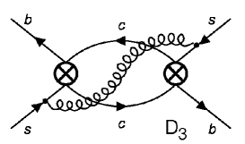
Figure 1: The imaginary part of massive two loop diagram of that form has to be calculated.

One can do the calculation in two different ways (we did it in both ways, to have a check):

• calculate the imaginary part of the two loop integrals

or

• use Cutkosky rules and calculate virtual and real one loop corrections, followed by a phase space integration.

The result in LO QCD has the following form

$${\cal T}=-\frac{G_{F}^{2}m_{b}^{2}}{12\pi}\left(V_{cb}^{*}V_{cs}\right)^{2}\left[G(z)Q+G_{S}(z)Q_{S}\right]$$ (18)

with $z=m_{c}^{2}/m_{b}^{2}$ and the $\Delta B=2$ operators

$$Q = (\bar{b}_{i}s_{i})_{V-A}(\bar{b}_{j}s_{j})_{V-A}$$

$$Q_{S} = (\bar{b}_{i}s_{i})_{S-P}(\bar{b}_{j}s_{j})_{S-P}\;.$$ (19)

In principle we have more operators, but we can reduce them to the two operators above with the use of Fierz identities .
Equation (18) is an example of an operator product expansion of equation (16). We have reduced the double insertion of $\Delta B=1$ operators, which appear in ${\cal H}_{eff}$, to a single insertion of an $\Delta B=2$ operator. In principle we have integrated out the internal charm quarks in figure 1.
For the NLO calculation we have to match the $\Delta B=1$ double insertion with gluon exchange to a $\Delta B=2$ insertion with gluon exchange. This means, we have to calculate the following diagrams:

Figure 2: All diagrams that have to be calculated for the NLO QCD determination of $\Delta\Gamma_{B_{s}}$.

These diagrams can be classified in the following way:

1. Virtual one loop corrections to a $\Delta B=2$ operator insertion.

2. Imaginary part of virtual two loop corrections to a double insertion of $\Delta B=1$ operators.

3. Penguin contributions to the $\Delta B=1$ double insertion.

The calculation of all these diagrams gives us the NLO QCD result.

4 Results

The result in NLO is:

$${\cal T}=-\frac{G_{F}^{2}m_{b}^{2}}{12\pi}\left(V_{cb}^{*}V_{cs}\right)^{2}\left[G(z)Q-G_{S}(z)Q_{S}\right]$$ (20)

with the following numerical values for the Wilson coefficients

$$\begin{array}[]{|c|c|c|c|}\hline\cr\mu&m_{b}/2&m_{b}&2m_{b}\\ \hline\cr G^{(0)}&0.013&0.047&0.097\\ \hline\cr G&0.023&0.030&0.036\\ \hline\cr G^{(0)}_{S}&1.622&1.440&1.292\\ \hline\cr G_{S}&0.743&0.937&1.018\\ \hline\cr\end{array}$$

with

$$G=G^{(0)}+\frac{\alpha}{4\pi}G^{(1)}\;.$$ (21)

Here one can see two important points. First, the value for $G_{S}$ is numerical dominant and second, the NLO values are considerably smaller than the LO values.

For the final result we parametrise the matrix elements of the $\Delta B=2$ operators in the following way:

$$\langle\bar{B}_{s}|Q|B_{s}\rangle = \frac{8}{3}f^{2}_{B_{s}}M^{2}_{B_{s}}B$$

$$\langle\bar{B}_{s}|Q_{S}|B_{s}\rangle = -\frac{5}{3}f^{2}_{B_{s}}M^{2}_{B_{s}}\frac{M^{2}_{B_{s}}}{(\bar{m}_{b}+\bar{m}_{s})^{2}}B_{S}\;.$$

$B$ and $B_{S}$ are so-called bag parameters, $f_{B_{s}}$ is the decay constant. The values of these parameters have to be determined by non-perturbative methods like lattice simulations. $\bar{m}_{q}$ denotes the running quark mass in the $\overline{MS}$-scheme.

With the following input parameters

$$m_{b}=4.8\mbox{GeV}\;\;\;\;\left(\frac{m_{c}}{m_{b}}\right)^{2}=0.085\;\;\;\;\bar{m}_{s}=0.2\mbox{GeV}$$

$$M_{B_{s}}=5.37\mbox{GeV}\;\;\;\;B(B_{s}\mapsto Xe\nu)=0.104$$ (22)

we obtain for the relative dacay rate difference

$$\framebox{$\begin{array}[]{ccl}\left(\frac{\Delta\Gamma}{\Gamma}\right)_{B_{s}}&=&\left(\frac{f_{B_{s}}}{210\mbox{MeV}}\right)^{2}\\ &&\\ &&\left[0.006B(m_{b})+0.150B_{S}(m_{b})-0.063\right]\end{array}$}\;.$$

A definitive determination of the two bag parameters is still missing. From the literature [15] we were able to extract preliminary values for the bag parameters

$$B(m_{b})=0.9\;\;\;\;\;\;\;\;B_{S}(m_{b})=0.75\;.$$ (23)

With that numbers at hand we obtain as a final result

$$\framebox{$\displaystyle\left(\frac{\Delta\Gamma}{\Gamma}\right)_{B_{s}}=\left(\frac{f_{B_{s}}}{210\mbox{MeV}}\right)^{2}\left(0.054^{+0.016}_{-0.032}\pm???\right)$}\;.$$ (24)

The question marks remind us that we do not know the uncertainties in the numerical values for the bag parameters.

5 Disscussion and outlook

The LO estimate for the relative decay rate difference ${\Delta\Gamma_{B_{s}}/\Gamma_{B_{s}}={\cal{O}}(20\%)}$ is considerably reduced due to several effects:

• the $1/m_{b}$ corrections are sizeable and give an absolute reduction of about - 6.3 % [9].

• the pure NLO QCD corrections are sizeable, too and give an absolute reduction of about - 4.8 % [10].

• with the NLO QCD corrections at hand we can perform a proper matching to the (preliminary) lattice calculations for the bag parameters. This tells us that we have to use a low value for the bag parameters, i.e. $B_{S}(m_{b})=0.75$ [10, 15]. Compared to the naive estimate $B_{S}=1$, this is another absolute reduction of about - 3.8 %.

Unfortunateley the value of $\Delta\Gamma_{B_{s}}/\Gamma_{B_{s}}$ has been pinned down to a value of about $5\%$. The LO prediction was just a the border of experimental visibility [7]. Now we will have to wait for the forthcoming experiments like HERA-B, Tevatron (run II) and LHC.

Another application of our calculation are inclusive indirect CP-asymmetries in the $b\to u\bar{u}d$ channel. For the complete NLO prediction of this quantity, $\Gamma_{12}$ in the $B_{d}$ system was missing. We get this value from our calculation with a trivial exchange of the CKM parameters and the limit $m_{c}\mapsto 0$. This allows a determination of the CKM-angle $\alpha$ [10, 16].

Acknowledgements. I want to thank the organizers of the Corfu Summer Institute on Elementary Particle Physics for their successful work, M. Beneke, G. Buchalla, C. Greub and U. Nierste for the pleasant collaboration and A.J. Buras for proofreading the manuscript.

References

• [1] A.Ali, these proceedings.
• [2] Branco, these proceedings.
• [3] Bertolini, these proceedings.
• [4] R. RΓΌckl, these proceedings.
• [5] J.H. Christenson, J.W. Cronin, V. L. Fitch and R. Turlay, Phys. Rev. Lett. 13, (1964), 138.
• [6] J.S. Hagelin, Nucl. Phys. B193, (1981), 123; E. Franco, M. Lusignoli and A. Pugliese, Nucl. Phys. B194, (1982), 403; L.L. Chau, Phys. Rep. 95, (1983), 1; A.J. Buras, W. SΕ‚ominski and H. Steger, Nucl. Phys. B245, (1984), 369; M.B. Voloshin, N.G. Uraltsev, V.A. Khoze and M.A. Shifman, Sov. J. Nucl. Phys. 46, (1987), 112; A. Datta, E.A. Paschos and U. TΓΌrke, Phys. Lett. B196, (1987), 382; A. Datta, E.A. Paschos and Y.L. Wu, Nucl. Phys. B311, (1988), 35.
• [7] K. Hartkorn and H.-G. Moser, MPI-PhE/98-21, appears in European Physical Journal C.
• [8] I. Dunietz, Phys. Rev. D52, (1995), 3048. R. Fleischer and I. Dunietz, Phys. Lett. B387, (1996), 361; Phys. Rev. D55, (1997), 259.
• [9] M. Beneke, G. Buchalla and I. Dunietz, Phys. Rev. D54, (1996), 4419.
• [10] M. Beneke, G. Buchalla, C. Greub, A. Lenz and U. Nierste, hep-ph/9808385; to appear in Phys. Lett. B.
• [11] Y. Grossman, Phys. Lett. B380, 99 (1996).
• [12] I. Bigi and N. Uraltsev, Phys. Lett. B280, (1992), 271.
• [13] I. Bigi, M. Shifman, N. Uraltsev, A. Vainshtein Phys.Rev. D59, (1999), 054011.
• [14] G. Buchalla, A.J. Buras and M.E. Lautenbacher, Rev. Mod. Phys. 68, (1996), 1125.
• [15] R. Gupta, T. Bhattacharya and S.R. Sharpe, Phys. Rev. D55, (1997), 4036.
J.M. Flynn and C.T. Sachrajda, [hep-lat/9710057], in Heavy Flavours (2nd ed.), eds. A.J. Buras and M. Lindner, World Scientific, Singapore.
• [16] M. Beneke, G. Buchalla and I. Dunietz, Phys. Lett. B393, (1997), 132.