Heavy Quark Production in DIS and Hadron Colliders

Abstract

We provide a brief overview of some current experimental and theoretical issues of heavy quark production.

1 Introduction

The production of heavy quarks in high energy processes has become an increasingly important subject of study both theoretically and experimentally. The theory of heavy quark production in perturbative Quantum Chromodynamics (pQCD) is more challenging than that of light parton (jet) production because of the new physics issues brought about by the additional heavy quark mass scale. The correct theory must properly take into account the changing role of the heavy quark over the full kinematic range of the relevant process from the threshold region (where the quark behaves like a typical “heavy particle”) to the asymptotic region (where the same quark behaves effectively like a massless parton). With steadily improving experimental data on a variety of processes sensitive to the contribution of heavy quarks (including the direct measurement of heavy flavor production), this is a very rich field for studying different aspects of the QCD theory including the problems of multiple scales, summation of large logarithms, subtleties of renormalization, and higher order corrections. We shall briefly review a limited subset of these issues.

2 The Factorization Theorem

Perturbative calculations for heavy quark production are performed in the context of the factorization theorem expressed below in the commonly used form:

$$\sigma_{a\to c} = f_{a\to b}(x,\mu^{2})\otimes\hat{\sigma}_{b\to c}(Q^{2}/\mu^{2},M_{H}^{2}/\mu^{2},\alpha_{s}(\mu))+{\cal O}(\Lambda^{2}_{QCD}/Q^{2})$$ (1)

While the factorization was originally proven for massless quarks,[2] the theorem has recently been extended by Collins[3] to incorporate quarks of any mass, including “heavy quarks.” (Note, we have explicitly retained the $M_{H}^{2}$ dependence in $\hat{\sigma}$.) It is important to note that the corrections to the factorization are only of order $\Lambda^{2}_{QCD}/Q^{2}$, and not $M_{H}^{2}/Q^{2}$, even for the case of general quark masses.

The factorization theorem can also be expressed as a composition of $t$-channel two particle irreducible (2PI) amplitudes:

$$\sigma_{a\to c} \simeq \hat{\sigma}_{b\to c}\otimes f_{a\to b}\simeq\left[C\cdot\frac{1}{1-(1-Z)K}\right]\cdot Z\ \cdot\ \left[\frac{1}{1-K}\cdot T\right]$$ (2)

Here, C represents the graph for a hard scattering, K represents the graph for a rung, T represents the graph that couples to the target, and Z represents a collinear projection operator. The first term in brackets roughly corresponds to the hard scattering coefficient function $\hat{\sigma}$, and the second term to the parton distribution function (PDF), $f$. Note that these two terms only communicate through a collinear projection operator, Z. Part of the effort in generalizing the factorization theorem for the case of massive quarks involves constructing the proper Z, and demonstrating that terms containing (1-Z) are power suppressed. However, once Z is determined, Eq.(2) yields an all-orders prescription for computing both the hard scattering coefficient ($\hat{\sigma}$) and the parton distribution function ($f$). A calculation using this formalism was first performed by ACOT[4] for the case of heavy quark production in deeply inelastic scattering, and we now examine this process in detail.

3 Heavy Quark Production in DIS

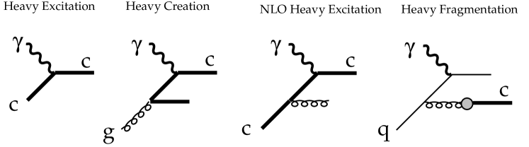
Figure 1: Basic processes for DIS heavy quark production. a) ${\cal O}(\alpha_{s}^{0})$ flavor excitation: $\gamma+c\to c$; b) ${\cal O}(\alpha_{s}^{1})$ flavor creation: $\gamma+g\to c+\bar{c}$; c) ${\cal O}(\alpha_{s}^{1})$ flavor excitation: $\gamma+c\to c+g$; d) ${\cal O}(\alpha_{s}^{1})$ light-quark ($q$) fragmentation: $(\gamma+q\to q+g)\otimes(g\to c)$.

Several experimental groups[5] have studied the semi-inclusive deeply inelastic scattering (DIS) process for heavy-quark production $\ell_{1}+N\to\ell_{2}+Q+X.$ New data from HERA investigates the DIS process in a very different kinematic range from that available at fixed-target experiments. This perception has changed the way that we compute the semi-inclusive DIS heavy quark production. Traditionally, the heavy quark mass was treated as a large scale, and the number of active parton flavors was fixed to be the number of quarks lighter than the heavy quark. In this scheme, the perturbation expansion begins with the ${\cal O}(\alpha_{s}^{1})$ heavy quark creation fusion process $\gamma g\to c\bar{c}$, (cf., Fig. 1b). We refer to this approach as the Fixed Flavor Number (FFN) scheme since the number of flavors coming from parton distributions is fixed at three for charm production.

More recently, a Variable Flavor Number (VFN) scheme (ACOT[4]) has been proposed which includes the heavy quark as an active parton flavor with non-zero heavy quark mass. In this case, the perturbation expansion begins with the ${\cal O}(\alpha_{s}^{0})$ heavy quark excitation process $\gamma c\to c$, (cf., Fig. 1a). The key advantages of this scheme are:[7]

1. By incorporating the heavy quark into the parton framework, the composite scheme yields a result which is valid from threshold to asymptotic energies; in contrast, the FFN scheme contains unsubtracted mass singularities which will vitiate the perturbation expansion in the $m_{c}\to 0$ or $E\to\infty$ limit.

2. Because the composite scheme resums the large logarithms appearing in the FFN scheme into the parton distribution functions, it includes the numerically dominant terms of the ${\cal O}(\alpha_{s}^{2})$ FFN scheme calculation in a ${\cal O}(\alpha_{s}^{1})$ calculation.

   

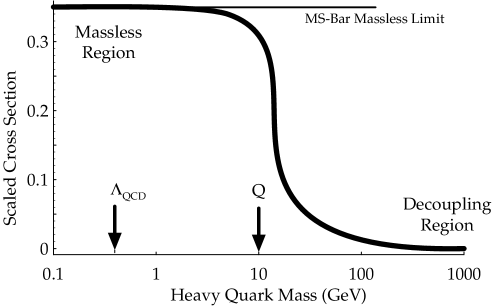
   Figure 2: The scaled cross section for DIS heavy quark production as a function of the quark mass $m_{H}$.

In effect, the VFN scheme subsumes the FFN scheme. To illustrate this fact with a concrete calculation, in Fig. 2, we plot the cross section for “heavy” quark production as a function of the quark mass. This figure clearly shows the three important kinematic regions. 1) In the massless region, where $m_{H}\ll Q$, the ACOT VFN result reduces precisely to the massless $\overline{{\rm MS}}$ result. 2) In the decoupling region, where $m_{H}\gg Q$, this “heavy quark” decouples and its contribution vanishes. 3) In the transition region, where $m_{H}\sim Q$, this (not-so) “heavy quark” plays an important dynamic role. While the FFN scheme is appropriate only when $m_{H}\,\lower 2.15277pt\hbox{$\stackrel{{\scriptstyle>}}{{\sim}}$}\,Q$, we see that the VFN scheme is valid throughout the full kinematic range.

Figure 3: The contributions to DIS charged current inclusive $F_{2}^{charm}$ vs. $\mu$. For each separate contribution, the thick lines are the $\overline{{\rm MS}}$ result ($m_{s}=0$), and the thin lines are the ACOT result with $m_{s}=0.5$ GeV. From Kretzer, Ref. [8].

This point is also illustrated in a calculation by Kretzer[8] (cf., Fig. 3) which shows the partial contributions to the charged current $F_{2}^{charm}$. In this figure, each line is actually a pair of lines: the thin lines represents the result for $F_{2}^{charm}$ using the ACOT scheme with $m_{s}=0.5$ GeV, and the thick lines regularize the strange quark with the massless $\overline{{\rm MS}}$ prescription. (The charm mass is, of course, retained.) The fact that these two calculations match so closely (particularly in comparison to the $\mu$-variation) indicates: 1) the ACOT scheme smoothly reduces to the desired massless $\overline{{\rm MS}}$ limit as $m_{H}\to 0$, and 2) for $m_{H}\,\lower 2.15277pt\hbox{$\stackrel{{\scriptstyle<}}{{\sim}}$}\,\Lambda_{QCD}$ we see that the quark mass no longer plays a dynamic role in the process and becomes purely a regulator.

4 Heavy Quarks and Extraction of $s(x)$

A topic closely related to DIS charm production is the extraction of the strange quark distribution.[10] In principle, we can extract $s(x)$ by comparing DIS neutral and charged current data. To leading order, we have:

$$\frac{F_{2}^{NC}}{F_{2}^{CC}} \simeq \frac{5}{18}\ \left\{1-\frac{3}{5}\frac{(s+\bar{s})-(c+\bar{c})+...}{q+\bar{q}}\right\}\quad.$$ (3)

While the individual $F_{2}$ structure functions are measured precisely (cf., Fig. 4),[11] this approach is indirect in the sense that small uncertainties in the larger valence distributions will magnify the uncertainty on the extracted $s(x)$.

A direct method of obtaining $s(x)$ is to use the neutrino induced di-muon process: $\nu_{\mu}N\to\mu^{-}cX$ with the subsequent decay $c\to s\mu^{+}\nu_{\mu}$. Here, the di-muon signal is directly related to the charm production rate, which goes via the process $W^{+}s\to c$ at leading order. The method has the advantage that the signal from the $s$-quark is not a small effect beneath the valence process.

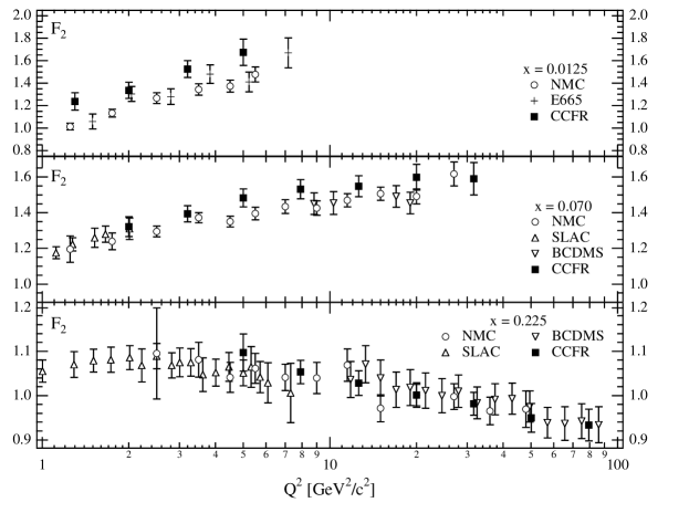
Figure 4: Comparison of $F_{2}$ from charged and neutral current DIS. From Seligman, et al., Ref. [11].

A complete NLO experimental analysis was performed using the CCFR data set.[13] The recently collected data from the NuTeV experiment will provide an opportunity to extend the precision of these investigations still further.[14] Their high intensity sign-selected neutrino beam and the new calibration beam allows for large improvement in the systematic uncertainty while minimizing statistical errors.[15]

5 Hadroprodution of Heavy Quarks

We now turn to the hadroproduction of heavy quarks, and discuss how the method of ACOT[4, 16] is used to provide a dynamic role for the heavy quark parton. We concentrate mostly on b-production at the Tevatron for definiteness, and present typical results for $b$ quark production.[1, 17, 18, 19] (See the paper by D. Fein, this meeting.[20]) Fig. 5a shows the scaled differential cross section vs. $p_{T}$ for $b$ production at 1800 GeV for the leading order (LO) calculations. The heavy creation (HC) process ($gg\to b\bar{b}$) represents the LO contribution to the fixed-flavor-number (FFN) scheme result. The heavy excitation (HE) process ($gb\to gb$) plus the HC term represents the LO contribution to the variable-flavor-number (VFN) scheme result. The pair of lines for each result shows the effect of varying $\mu$. In a similar manner, Fig. 5b shows the total FFN and VFN results.

Two interesting features are worth noting. 1) Examining Fig. 5a we observe the HE contribution is comparable to the HC one, in spite of the smaller $b$-quark PDF compared to the gluon distribution. Closer examination reveals that two effects contribute to this unexpected result: a larger color factor and the presence of $t$-channel gluon exchange diagrams for the HE process, as compared to the HC process. 2) The LO-VFN (=HC+HE) contributions (Fig. 5a) (tree processes) give a reasonable approximation to the full cross section TOT-VFN (Fig. 5b); thus, the NLO-VFN correction is relatively small. This is in sharp contrast to the familiar FFN scheme where the TOT-FFN term is more than twice as large as the LO-FFN (=HC). This is, of course, an encouraging result, suggesting that the VFN scheme heavy quark parton picture represents an efficient way to organize the perturbative QCD series.

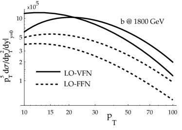
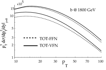
Figure 5: The scaled cross section ($nb$-GeV³) vs. $p_{T}$ for the a) LO-FFN and LO-VFN contributions, and b) TOT-FFN and TOT-VFN contributions. For each contribution, we choose $\mu=[M_{T}/2,2M_{T}]$, with $M_{T}=\sqrt{m_{H}^{2}+p_{T}^{2}}$, to gauge the $\mu$-variation. From Ref. [16].

In Fig. 5a, we also observe that while the TOT-VFN result provides minimal $\mu$-variation for low $p_{T}$, the improvement is decreased for large $p_{T}$. This may be, in part, due to that fact that the TOT-VFN result shown here is missing the NLO-HE process $gb\to ggb$ since this calculation, with masses retained, does not exist. In a separate effort, Cacciari and Greco[24] have used a NLO fragmentation formalism to resum the heavy quark contributions in the limit of large $p_{T}$. This calculation effectively includes the massless limit of the $gb\to ggb$ contribution (omitted above); the result is a decreased $\mu$-variation in the large $p_{T}$ region. Recently, this calculation has been merged with the massive FFN calculation by Cacciari, Greco, and Nason, (Ref. CGN); the result is a calculation which matches the FFN calculation at low $p_{T}$, and takes advantage of the NLO fragmentation formalism in the high $p_{T}$ region.

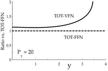
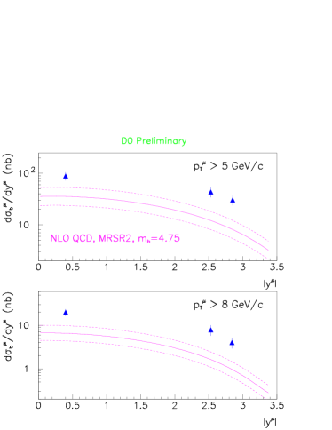
Figure 6: a) Comparison of the total cross section $d\sigma/dp_{t}^{2}/dy$ in the VFN and FFN formalism vs. $y$ for $b$ production at 1800 GeV with $p_{t}=20$ GeV and $\mu=M_{T}$. The curves are scaled by the total FFN cross section to facilitate comparison of the relative magnitude. From Ref. [16]. b) The measured differential muon cross sections from $b$ production and decay as a function of $y$. The Solid curve is a TOT-FFN prediction with dashed curves representing the theoretical uncertainties. Preliminary results from Ref. [18].

Not only do the VFN and FFN schemes yield different cross sections, but the differential distributions can be quite distinct. Specifically, in Fig. 6a we display the rapidity distribution for TOT-VFN as compared with the TOT-FFN result. We observe that the VFN scheme yields a broader rapidity distribution than the FFN scheme; in part, this is expected as the VFN result includes a t-channel gluon exchange process ($g+b\to g+b$) which can give an enhanced contribution in the forward direction. It is interesting to compare this result with the data; Fig. 6b. shows the comparison with the TOT-FFN result. In the central region, the TOT-FFN theory is a factor of $\sim$2 below the data; this increases to about a factor of $\sim$3 in the forward region. The TOT-VFN scheme increases (as compared to the TOT-FFN result) at large rapidity, as do the data. This observation suggests that the VFN scheme (which includes the flavor excitation process $g+b\to g+b$), provides a mechanism that can help resolve the $y$ shape discrepancy.

6 Massive vs. Massless Evolution

In a consistently formulated pQCD framework incorporating non-zero mass heavy quark partons, there is still the freedom to define parton distributions obeying either mass-independent or mass-dependent evolution equations. With properly matched hard cross-sections, different choices merely correspond to different factorization schemes, and they yield the same physical cross-sections. We demonstrate this principle in a concrete order $\alpha_{s}$ calculation of the DIS charm structure function.[26] In Fig. 7 we display the separate contributions to $F_{2}^{charm}$ for both mass-independent and mass-dependent evolution. The matching properties are best examined by comparing the (scheme-dependent) heavy excitation $F_{2}^{HE}$ and the subtraction $F_{2}^{SUB}$ contributions of Fig. 7a.

We observe the following. 1) Within each scheme, $F_{2}^{HE}$ and $F_{2}^{SUB}$ are well matched near threshold, cf., Fig. 7a. Above threshold, they begin to diverge, but the difference $(F_{2}^{HE}-F_{2}^{SUB})$, which contributes to $F_{2}^{TOT}$, is insensitive to the different schemes. 2) It is precisely this matching of $F_{2}^{HE}$ and $F_{2}^{SUB}$ which ensures the scheme dependence of $F_{2}^{TOT}$ is properly of higher-order in $\alpha_{s}$, (cf., Fig. 7b).

This matching is not accidental, but simply a result of using a consistent renormalization scheme for both $F_{2}^{HE}$ and $F_{2}^{SUB}$. To understand this we expand these terms near threshold ($\mu\sim m_{H}$) where the $m_{H}/Q$ terms are relevant:

$$\sigma_{SUB} = {}^{R}f_{g/P}\otimes{}^{R}\widehat{\sigma}^{(1)}_{g\gamma^{*}\to c\bar{c}}={}^{R}f_{g/P}\otimes\frac{\alpha_{s}}{2\pi}\int_{m_{H}^{2}}^{\mu^{2}}\frac{d\mu^{2}}{\mu^{2}}\ {}^{R}P^{(1)}_{g\to c}\otimes\sigma^{(0)}_{c\gamma^{*}\to c}+0$$

$$\sigma_{HE} \simeq {}^{R}f_{c/P}\otimes{}^{R}\widehat{\sigma}^{(0)}_{c\gamma^{*}\to c}\simeq{}^{R}f_{g/P}\otimes\frac{\alpha_{s}}{2\pi}\int_{m_{H}^{2}}^{\mu^{2}}\frac{d\mu^{2}}{\mu^{2}}\ {}^{R}P^{(1)}_{g\to c}\otimes\sigma^{(0)}_{c\gamma^{*}\to c}+{\cal O}(\alpha_{s}^{2})$$

Here, the prescript $R$ specifies the renormalization scheme. From these relations, it is evident that $F_{2}^{HE}$ and $F_{2}^{SUB}$ will match to ${\cal O}(\alpha_{s}^{2})$ so long as a consistent choice or renormalization scheme $R$ is made for the splitting kernels, ${}^{R}P^{(1)}_{g\to c}$. This is the key mechanism that compensates the different effects of the mass-independent vs. mass-dependent evolution, and yields a $\sigma_{TOT}$ which is identical up to higher-order terms. The lesson is clear: the choice of a mass-independent $\overline{{\rm MS}}$ or a mass-dependent (non-$\overline{{\rm MS}}$) evolution is purely a choice of scheme, and becomes simply a matter of convenience–there is no physically new information gained from the mass-dependent evolution.

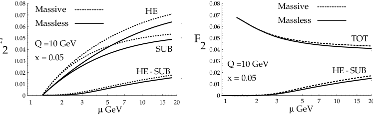
Figure 7: $F_{2}$ vs. $\mu$ for DIS c-production. a) $F_{2}^{HE}$, $F_{2}^{SUB}$ and the difference $(F_{2}^{HE}-F_{2}^{SUB})$. The solid curves are for the mass-independent evolution scheme, and the dashed curves are for the mass-dependent evolution scheme. b) $F_{2}^{TOT}$ and $F_{2}^{HE}-F_{2}^{SUB}$. The difference between the mass-independent evolution and mass-dependent evolution for $F_{2}^{TOT}$ is higher order and comparable or less than the $\mu$-variation. From Ref. [26].

7 Conclusions

We have provided a brief overview of some current experimental and theoretical issues of heavy quark production. The wealth of recent heavy quark production data from both fixed-target and collider experiments will allow us to to extract precise measurements of structure functions which can provide important constraints on searches for new physics at the highest energy scales. As an important physical process involving the interplay of several large scales, heavy quark production poses a significant challenge for further development of QCD theory.

We thank J.C. Collins, R.J. Scalise, and W.-K. Tung for valuable discussions, and the Fermilab Theory Group for their kind hospitality during the period in which part of this research was carried out. This work is supported by the U.S. Department of Energy and the Lightner-Sams Foundation.

References

- [1] S. Frixione, M. L. Mangano, P. Nason, and G. Ridolfi, hep-ph/9702287; M. L. Mangano, hep-ph/9711337.
- [2] J. Collins, D. Soper, and G. Sterman, Nucl. Phys. B250, 199 (1985).
- [3] J. C. Collins, Phys. Rev. D58, 094002 (1998).
- [4] M. A. G. Aivazis, J. C. Collins, F. I. Olness, and W.-K. Tung, Phys. Rev. D 50, 3102 (1994).
-
[5]
H1 Collaboration (C. Adloff et al.).
Z. Phys. C72, 593 (1996).
ZEUS Collaboration (J. Breitweg et al.). Talk given at International Europhysics Conference on High-Energy Physics (HEP 97), Jerusalem, Israel, 19-26 Aug 1997, N-645. - [6] E. Laenen, S. Riemersma, J. Smith, W.L. van Neerven. Phys. Rev. D49, 5753 (1994); M. Buza, Y. Matiounine, J. Smith, and W. L. van Neerven, hep-ph/9707263; hep-ph/9612398; M. Buza and W. L. van Neerven, Nucl. Phys. B500, 301 (1997).
- [7] C. Schmidt, hep-ph/9706496; J. Amundson, C. Schmidt, W. K. Tung, X. Wang, MSU preprint, in preparation.
- [8] S. Kretzer, e-Print hep-ph/9808464, S. Kretzer, I. Schienbein, Phys. Rev. D58, 094035 (1998).
- [9] R.S. Thorne, R.G. Roberts, Phys. Lett. B421, 303 (1998); R.S. Thorne, R.G. Roberts, Phys. Rev. D57, 6871 (1998).
- [10] H. L. Lai et al., Phys. Rev. D 55, 1280 (1997); H. L. Lai et al., hep-ph/9903282.
- [11] CCFR Collaboration (W.G. Seligman et al.), Phys. Rev. Lett. 79, 1213 (1997).
- [12] Janet M. Conrad, Michael H. Shaevitz, and Tim Bolton. hep-ex/9707015
- [13] A. O. Bazarko et al., Z. Phys. C65, 189 (1995).
- [14] NuTeV Collaboration: Jaehoon Yu et al., hep-ex/9806030; K.S. McFarland et al., hep-ex/9806013.
- [15] T. Adams,Heavy Quark Production in Neutrino Deep-Inelastic Scattering. Proceedings of 4th Workshop on Heavy Quarks at Fixed Target (HQ 98), Batavia, IL, 10-12 Oct 1998. p.198.
- [16] F.I. Olness, R.J. Scalise, Wu-Ki Tung, hep-ph/9712494. Phys. Rev. D59, 014506 (1999).
- [17] CDF Collaboration (F. Abe et al.), Phys. Rev. D 50, 4252 (1994); Phys. Rev. Lett. 75, 1451 (1995).
- [18] D0 Collaboration (S. Abachi et al.), Phys. Rev. Lett. 74, 3548 (1995).
- [19] A. Zieminski,B Production and Onium production at the Tevatron. Proceedings of 4th Workshop on Heavy Quarks at Fixed Target (HQ 98), Batavia, IL, 10-12 Oct 1998. p.218.
- [20] D. Fein,B-cross sections: 1800/630, rapidity dependence, onium. Hadron13, Mumbai, India, January 14-20, 1999.
- [21] P. Nason, S. Dawson, and R. K. Ellis, Nucl. Phys. B303, 607 (1988); B327, 49 (1989); B335, 260(E) (1990).
- [22] W. Beenakker, H. Kuijf, W. L. van Neerven, and J. Smith, Phys. Rev. D 40, 54 (1989); W. Beenakker, W. L. van Neerven, R. Meng, G. A. Schuler, and J. Smith, Nucl. Phys. B351, 507 (1991).
- [23] M. L. Mangano, P. Nason, and G. Ridolfi, Nucl. Phys. B373, 295 (1992).
- [24] M. Cacciari and M. Greco, Nucl. Phys. B421, 530 (1994).
- [25] M. Cacciari, M. Greco, and P. Nason, hep-ph/9803400, J. High Energy Phys. 05, 007 (1998).
- [26] F. I. Olness and R. J. Scalise, Phys. Rev. D 57, 241 (1998).