decays in supersymmetry
E. Lunghi, A. Masiero,
SISSA-ISAS, Via Beirut 2-4, Trieste, Italy and
INFN, Sezione di Trieste, Trieste, Italy
I. Scimemi
Dep. de Fisica Teorica, Univ. de Valencia,
c. Dr.Moliner 50, E-46100, Burjassot, Valencia, Spain
and
L. Silvestrini
Physik Department, Technische Universität München,
D-85748 Garching, Germany
Ref. SISSA-17/99/EP
Ref. TUM-HEP-346/99
Ref. FTUV/99-30
IFIC/99-32
We study the semileptonic decays , in generic supersymmetric extensions of the Standard Model. SUSY effects are parameterized using the mass insertion approximation formalism and differences with the Constrained MSSM results are pointed out. Constraints on SUSY contributions coming from other processes (e.g. ) are taken into account. Chargino and gluino contributions to photon and Z-mediated decays are computed and non-perturbative corrections are considered. We find that the integrated branching ratios and the asymmetries can be strongly modified. Moreover, the behavior of the differential Forward-Backward asymmetry remarkably changes with respect to the Standard Model expectation.
1 Introduction
One of the features of a general low energy supersymmetric (SUSY) extension of the Standard Model (SM) is the presence of a huge number of new parameters. FCNC and CP violating phenomena constrain strongly a big part of the new parameter space. However there is still room for significant departures from the SM expectations in this interesting class of physical processes. It is worthwhile to check all these possibilities on the available data and on those processes that are going to be studied in the next future. In this way it is possible to indicate where new physics effects can be revealed as well as to establish criteria for model building.
In this work we want to investigate the relevance of new physics effects in the semileptonic inclusive decay . This decay is quite suppressed in the Standard Model; however, new -factories should reach the precision requested by the SM prediction [1] and an estimate of all possible new contributions to this process is compelling.
Semileptonic charmless decays have been deeply studied. The dominant perturbative SM contribution has been evaluated in ref. [2] and later two loop QCD corrections have been provided [3, 4]. The contribution due to resonances to these results are included in the papers listed in ref. [5]. Long distance corrections can have a different origin according to the value of the dilepton invariant mass one considers. corrections have been first calculated in ref. [6] and recently corrected in ref. [7, 8]. Near the peaks, non-perturbative contributions generated by resonances by means of resonance-exchange models have been provided in ref. [7, 9]. Far from the resonance region, instead, ref. [10] (see also ref. [11]) estimate long-distance effects using a heavy quark expansion in inverse powers of the charm-quark mass ( corrections).
An analysis of the SUSY contributions has been presented in refs. [12]–[15] where the authors estimate the contribution of the Minimal Supersymmetric Standard Model (MSSM). They consider first a universal soft supersymmetry breaking sector at the Grand Unification scale (Constrained MSSM) and then partly relax this universality condition. In the latter case they find that there can be a substantial difference between the SM and the SUSY results in the Branching Ratios and in the forward–backward asymmetries. One of the reasons of this enhancement is that the Wilson coefficient (see section 2 for a precise definition) can change sign with respect to the SM in some region of the parameter space while respecting constraints coming from . The recent measurements of [16] have narrowed the window of the possible values of and in particular a sign change of this coefficient is no more allowed in the Constrained MSSM framework. Hence, on one hand it is worthwhile considering in a more general SUSY framework then just the Constrained MSSM, and, on the other hand, the above mentioned new results prompt us to a reconsideration of the process. In reference [17] the possibility of new-physics effects coming from gluino-mediated FCNC is studied. Effects of SUSY phases in models with heavy first and second generation sfermions have been recently discussed in ref. [18].
We consider all possible contributions to charmless semileptonic decays coming from chargino-quark-squark and gluino-quark-squark interactions and we analyze both Z-boson and photon mediated decays. Contributions coming from penguin and box diagrams are taken into account; moreover, corrections to the mass insertion approximation (see below) results due to a light are considered. A direct comparison between the SUSY and the SM contributions to the Wilson coefficients is performed. Once the constraints on mass insertions are established, we find that in generic SUSY models there is still enough room in order to see large deviations from the SM expectations for branching ratios and asymmetries. For our final computation of physical observables we consider NLO QCD evolution of the coefficients and non-perturbative corrections (…), each in its proper range of the dilepton invariant mass.
Because of the presence of so many unknown parameters (in particular in the scalar mass matrices) which enter in a quite complicated way in the determination of the mass eigenstates and of the various mixing matrices it is very useful to adopt the so-called “Mass Insertion Approximation”(MIA) [19]. In this framework one chooses a basis for fermion and sfermion states in which all the couplings of these particles to neutral gauginos are flavor diagonal. Flavor changes in the squark sector are provided by the non-diagonality of the sfermion propagators. The pattern of flavor change is then given by the ratios
| (1) |
where are the off-diagonal elements of the mass squared matrix that mixes flavor , for both left- and right-handed scalars (Left, Right) and is the average squark mass (see e.g. [20]). The sfermion propagators are expanded in terms of the s and the contribution of the first two terms of this expansion are considered. The genuine SUSY contributions to the Wilson coefficients will be simply proportional to the various s and a keen analysis of the different Feynman diagrams involved will allow us to isolate the few insertions really relevant for a given process. In this way we see that only a small number of the new parameters is involved and a general SUSY analysis is made possible. The hypothesis regarding the smallness of the s and so the reliability of the approximation can then be checked a posteriori.
Many of these s are strongly constrained by FCNC effects [20, 21, 22] or by vacuum stability arguments [23]. Nevertheless it may happen that such limits are not strong enough to prevent large contributions to some rare processes. For instance it has been recently found in ref. [24] that the off-diagonal squark mass matrix elements can enhance rare kaon decays by roughly an order of magnitude with respect to the SM result.
The paper is organized as follows. In sect. 2 we define the operator basis, the basic formulae for the BR, the Forward–Backward asymmetry and the non-perturbative corrections. Sect. 3 and sect. 4 treat chargino and gluino contributions in the mass insertion approximation. The light corrections are presented in sect. 5. Constraints on s are discussed in sect. 6 and final results and conclusions are drawn in sect. 7 and 8.

2 Operator basis and general framework
The effective Hamiltonian for the decay in the SM and in the MSSM is given by (neglecting the small contribution proportional to )
| (2) |
where
| (3) |
is the CKM-matrix and . This Hamiltonian is known at next-to-leading order both in the SM [3, 4] and in the MSSM [14, 15]. We find that the most general low-energy SUSY Hamiltonian also contains the operators
| (4) |
However it is shown in following sections that the contribution of these operators is negligible and so they are not considered in the final discussion of physical quantities. SUSY contributions to other operators are negligible because they influence our observables at an higher perturbative order.
With these definitions the differential branching ratio and the forward-backward asymmetry can be written as
| (5) | |||||
| (6) | |||||
where , is the angle between the positively charged lepton and the B flight direction in the rest frame of the dilepton system, and are the phase space factor and the QCD correction factor () that enter and can be found in refs. [4, 25]. includes all the contributions of the operators and and its complete definition for the SM and MSSM can be found again in refs. [3, 4, 14].
In the literature the energy asymmetry is also considered [14] but it is easy to show that these two kind of asymmetries are completely equivalent; in fact a configuration in the dilepton c.m.s. in which is scattered in the forward direction kinematically implies in the B rest frame (see for instance ref. [7]).
It is worth underlying that integrating the differential asymmetry given in eq. (6) we do not obtain the global Foward–Backward asymmetry which is by definition:
| (7) |
where and stand respectively for leptons scattered in the forward and backward direction.
To this extent it is useful to introduce the following quantity
| (8) |
whose integrated value is given by eq. (7).
Eqns. (5) and (6) have been corrected in order to include several non-perturbative effects. First of all effects have been estimated by [7],
| (9) | |||||
| (10) | |||||
where
and are the two parameters that appear in the Heavy Quark Expansion (HQE). While the value of is quite well-established, (, is not yet well known. In ref. [26] is estimated as GeV2 and in ref. [27] GeV2. In what follows we consider the weighted average of the two results GeV2. As was pointed out by the authors of ref. [7] these corrections are no more valid near the endpoint region, , where they diverge because of the breaking down of the HQE. Following some recent analyses we have stopped the BRs corrections given in eq. (9) at (see ref. [8]) and the ones in eq. (10) at (see ref. [7]).
In order to account for the corrections to the parton model approximation in the high region ref. [7] and ref. [8] adopt two different approaches. The former considers a Fermi-motion model and the latter invokes the Heavy Hadron Chiral Perturbation Theory (HHChPT). A discussion about the usefulness of the Fermi-motion model for semileptonic charmless -decays is beyond the scope of this paper. In order to have a model independent description of the high energy region of the spectrum we have considered the HHChPT corrections.
For the branching ratio is dominated by the exclusive decays and ; in ref. [8] is shown that the contribution of the latter is completely negligible. In the following we report the expression of the branching ratio, valid in the interval of the spectrum given above, computed in the HHChPT framework
| (11) | |||||
where
| (12) |
and the definitions of can be found in ref. [8]. Moreover, we have put g=0.5 according to the theoretical estimate given in ref. [28]. In the intermediate region we have interpolated the obtained results. The form factors and can be computed also using other methods ( QCD Sum Rules [29], Ligh Cone QCD Sum Rules [30], QCD relativistic potential model [31]) but the HHChPT approach is preferable in the endpoint region of the spectrum.
The asymmetries receive no contribution from the single kaon mode and the endpoint of their spectrum is fixed, instead, by at . In the region we use the parton model result because these asymmetries have not been computed yet in the HHChPT framework.
Finally, the following corrections occur for (see e.g. [10])
| (13) | |||||
| (14) | |||||
The and corrections to can be easily computed because of the following relation
| (15) |
All the effects coming from the mass insertion approximation can be included in formulae (5-14) writing the coefficients , , as
| (16) |
where all the contributions are evaluated at the scale and the various summarize all the contributions coming from graphs including SUSY Higgs bosons and sparticles in the limit in which we neglect all the mass insertion contributions (they would be the only SUSY diagrams if the scalar mass matrices were diagonalized by the same rotations as those needed by the fermions). The explicit expressions for can be found in ref. [14].
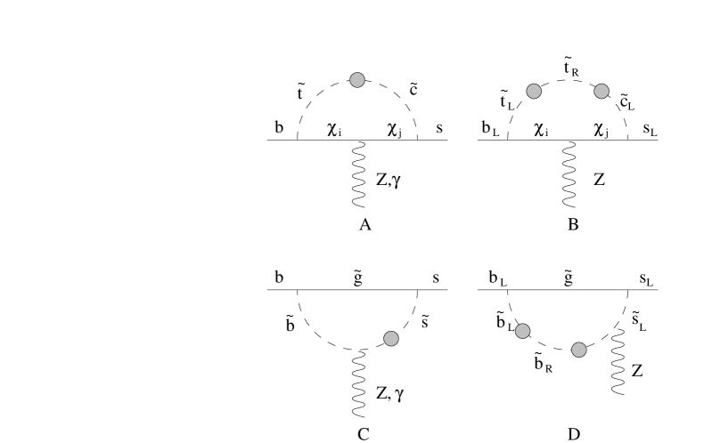
The Feynman diagrams with MI relevant for are drawn in figs 1-2. We have considered gluino-like and chargino-like contributions with both single and double mass insertions.
Both photons and Z-bosons can mediate the decay. Usually one finds that Z-boson contributions are dominant in those graphs where an “explicit breaking” is provided, i.e., both Left and Right squarks are present in the same loop. In the latter cases the photon cannot feel any gauge-symmetry-breaking and its contribution to the Wilson coefficients is suppressed by a factor with respect to the Z-boson one. For GeV, this factor amounts to about an order of magnitude. On the other hand if the graph does not give any explicit breaking we are in the opposite situation and the Z–boson contribution is suppressed by a factor . Moreover, a general feature of -mediated four fermion contributions is that, for high average squark masses, they decouple much faster than in the Z-boson case. This can be understood simply using dimensional arguments. While Wilson coefficients for Z-boson mediated four-fermion interactions are proportional to , the same coefficients must be proportional to for the ( here is a generic off–diagonal element of the sparticle squared mass matrices and it cannot rise as fast as for high values of ). Thus photon graphs can compete with Z-boson graphs if the sparticle spectrum is not too heavy.
Finally the value of the physical constants we use is reported in table 1.
| 173.8 GeV | |
| 4.8 GeV | |
| 1.4 GeV | |
| 125 MeV | |
| 5.27 GeV | |
| .119 | |
| 128.9 | |
| .2334 |
3 Chargino interactions
In the weak eigenstates basis the chargino mass matrix is given by
| (17) |
where the index 1 of rows and columns refers to the the wino state, the index 2 to the higgsino one, is the Higgs quadratic coupling and the soft SUSY breaking wino mass. In order to define the mass eigenstates the unitary matrices and which diagonalize are introduced,
After the rotation to mass eigenstates it is always possible to speak of wino-quark-squark or higgsino-quark-squark interactions. In order to identify the wino and higgsino states from the chargino ones it is sufficient to pick up the right elements from the and matrices. To be clear we write them explicitly for the cases of interest in the super-CKM basis. The wino-quark-squark, , vertex is ( and are a generic down-quark and up-squark)
| (18) |
and the higgsino-quark-squark, , vertex is
| (19) |
where is the CKM-matrix, , and are the Yukawa matrices for the up– and down–quarks.
Chargino graphs can contribute to the decay via both single and double insertions (see figs. 1-2). The double insertion is particularly convenient if the corresponding s are not very constrained [24]. In the following subsections we examine both the cases. In the case of a single insertion approximation both - and Z- mediated decays are considered.
In all what follows our results for the integrals are written in terms of the functions
| (20) |
To get a feeling with numbers it is sufficient to say that for ,
| (21) |
where is the Euler -function.
3.1 Single mass insertion –
The Z-boson mediated decay can proceed in two ways depending on the type of chargino-quark-squark vertices we consider. If an explicit breaking on the squark line of fig. 1A is required we must take both an higgsino and a wino vertex. In this way we get a contribution to the Wilson coefficients
| (22) |
where . This diagram, however, is exactly null in the limit in which , approximate the identity matrix and so it is negligible for high .
With two wino-quark-squark vertices we obtain
| (23) |
where we have retained only the contribution which arises because of the explicit breaking (with a double wino–higgsino mixing in the wino line); in fact eq. (23) is null in the limit of diagonal chargino mass matrix.
Graphs with two higgsino-quark-squark vertices are suppressed with respect to these ones by Yukawa or CKM factors.
3.2 Single mass insertion –
The contributions of the penguin with two wino vertices are
| (24) |
The contributions of the penguin with an higgsino and a wino vertices are
| (25) |
3.3 Single mass insertion – box
Finally we compute the contributions which come from chargino box diagrams of fig. 2.
In the wino exchange case the result is
| (26) |
where
| (27) |
and .
If the wino-bottom-stop vertex is replaced by an Higgsino-bottom-stop one we obtain
| (28) |
3.4 Double mass insertion – Z
It was recently pointed out [24] that a double mass insertion can provide a great enhancement of the SUSY contribution to the decay width, at least in the K-system case, if the s are not very constrained.
For B decay we obtain contributions from this graph to and ,
| (29) |
4 Gluino interactions
The main contribution of this kind of interactions comes from the graphs drawn in fig. 1C,D. In what follows we analyze the single and double mass insertion cases.
4.1 Single mass insertion –
The corrections to the coefficients in the photon mediated decay case are:
| (30) |
4.2 Single mass insertion – Z
The only relevant contributions to the Z-boson mediated decay width come from diagrams in which the Z feels directly the breaking of . According to the argument of section 2 all the diagrams that do not respect this condition are suppressed with respect to the photon mediated ones and can be neglected. However, for penguins containing a gluino, an explicit breaking can be provided only with a double MI. If only one MI is considered, Z-mediated decays are completely negligible with respect to the -mediated ones.
4.3 Double mass insertion – Z
For completeness we report here also the result obtained performing a double mass insertion in the gluino penguin.
| (31) |
5 Light effects
In the Mass Insertion Approximation framework we assume that all the diagonal entries of the scalar mass matrices are degenerate and that the off diagonal ones are sufficiently small. In this context we expect all the squark masses to lie in a small region around an average mass which we have chosen not smaller than 250 GeV. Actually there is the possibility for the to be much lighter; in fact the lower bound on its mass is about 70 GeV. For this reason it is natural to wonder how good is the MIA when a explicitly runs in a loop.
The diagrams, among those we have computed, interested in this effect are the chargino penguins and box with the insertion. To compute the light– contribution we adopt the approach presented in ref. [32]. There the authors consider an expansion valid for unequal diagonal entries which gives exactly the MIA in the limit of complete degeneration.
The new expressions for the contributions to the coefficients and are the following.
-
•
Chargino Z–penguin with both an higgsino and a wino vertex:
(32) where and the functions and can be found in ref [32].
-
•
Chargino –penguin with both an higgsino and a wino vertex:
(33) where
(34) - •
All the above formulas reduce exactly to those presented in sect. 3 in the limit .
6 Constraints on mass insertions
In order to establish how large the SUSY contribution to can be, one can compare, coefficient per coefficient, the MI results with the SM ones taking into account possible constraints on the s coming from other processes.
The most relevant s interested in the determination of the Wilson coefficients , and are , , , and .
-
•
Vacuum stability arguments regarding the absence in the potential of color and charge breaking minima and of directions unbounded from below [23] give
(36) For GeV this is not an effective constraint on the mass insertions.
-
•
A constraint on can come from the possible measure of .
In fact the gluino–box contribution to [22] is proportional to (see for instance ref. [22]). A possible experimental determination of , say
(37) would imply that
(38) for squark masses about . Moreover the LL up- and down-squark soft breaking mass matrices are related by a Cabibbo-Kobayashi-Maskawa rotation
(39) so that the limit (38) would be valid for the up sector too:
(40) -
•
Some constraints come from the measure of . The branching ratio of this process depends almost completely on the Wilson coefficients and which are proportional respectively to and . The most recent CLEO estimate of the branching ratio for is [16]
(41) where the first error is statistical, the second is systematic and the third comes from the model dependence of the signal. The limits given at 95% C.L. are [16]:
(42) We can define a as
(43) where can be found for instance in ref. [35]. Considering the experimental limits given in eq. (42) we find
(44) Actually and the constraint given in eq. (44) should be shared between the two coefficients. However in order to get the maximum SUSY contribution, we observe that in physical observables does not interfere with , the term is suppressed by a factor with respect to the one and is numerically negligible (in fact is much smaller than ). For these reasons we choose to fill the constraint of eq. (44) with alone.
The bounds (44) are referred to the coefficient evaluated at the scale while we are interested to the limits at the much higher matching scale. After the RG evolution has been performed we find that for an average squark mass lower than 1 TeV, the MIA contribution alone with a suitable choice of s, can always fit the experimental constraints.
Thus, since we are interested in computing the maximum enhancement (suppression) SUSY can provide, we can choose the total anywhere inside the allowed region given in eq. (44) still remaining consistent with the MIA.
The limit we get for is of order and this rules out Z-mediated gluino penguins contributions to and .
For what concerns we find that the constraint changes significantly according to the sign of . In this case it is important to consider both the positive and negative region as this delta can give a non negligible contribution to and . The limits depend on the choice of the parameters in the chargino sector; the numerical results given below are computed for GeV, GeV, GeV, (in sect. 7 we will show that these are the conditions under which we find the best SUSY contributions). Considering the positive interval we find while in the negative one .
-
•
Finally a comment on the s coming in graphs with a double MI is in order.
Given the constraints on one can see that the gluino-penguins with a double MI give negligible contributions to the final results even if is of order .
A of order , can give rise to light or negative squark mass eigenstates. In particular a light would contribute too much to the -parameter. Eventual model dependent cancelation can provide an escape to these constraints. In any case the numerical value of these contributions is not particularly important for the determination of physical observables. Since we want to provide a model independent analysis we prefer not to consider in our final computation these double insertion graphs and we present them only for completeness.
Contributions with three mass insertions are suppressed due to small loop integrals and to the various constraints on the deltas.
7 Results
The results of the calculations of sections 3-4 are presented in figs. 3-4 and in tables 7-7. While the gluino sector of the theory is essentially determined by the knowledge of the gluino mass (i.e. ), the chargino one needs two more parameters (i.e. , and ). Moreover it is a general feature of the models we are studying the decoupling of the SUSY contributions in the limit of high sparticle masses: we expect the biggest SUSY contributions to appear for such masses chosen at the lower bound of the experimentally allowed region. On the other hand this considerations suggest us to constrain the three parameters of the chargino sector by the requirement of the lighter eigenstate not to have a mass lower than the experimental bound of about 70 GeV [33]. The remaining two dimensional space has yet no constraint. For these reasons we scan the chargino parameter space by means of scatter plots for which , , and ; for every choice of these two parameters, is determined imposing to the lighter eigenstate a mass of about 70 GeV. In the plots we sum all contributions coming from different graphs proportional to a common mass insertion (the actual values of the coefficients are obtained multiplying the points in the plots by the MI).
In the tables we report the contribution of each diagram and the explicit dependence on the mass insertion parameters. We evaluate the coefficients varying and between 250 GeV and 1 TeV. The other parameters in tab. 7 are fixed from the scatter plots in order to give the best SUSY contributions to and .
Thus, with , GeV, GeV, , one gets
| (45) |
In order to numerically compare eq. (45) with the respective SM results we note that the minimum value of is about 4 while . Thus one deduces that SM expectations for the observables are enhanced when is positive. Moreover the big value of implies that the final total coefficient can have a different sign with respect to the SM estimate. As a consequence of this, the sign of asymmetries can be the opposite of the one calculated in the SM.
The diagonal contributions to , introduced in sect.2, and computed in the same range of the parameters (with chosen just above the experimental threshold of about ) are
| (46) |
The sign and the value of the coefficient has a great importance. In fact the integral of the BR (see eq. (5)) is dominated by the and term for low values of . In the SM the interference between and is destructive and this behavior can be easily modifed in the general class of models we are dealing with.
In the following, according to the discussion of sect. 6, we give the configurations of the various s for which we find the best enhancements and suppressions of the SM expectations.
-
•
Best enhancement.
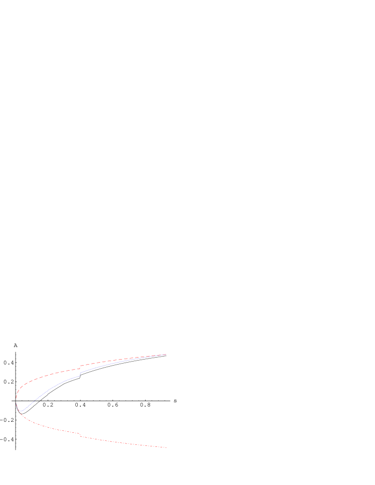
0.41 1.5 -8.3 -0.5 0.9 0.41 0.96 -2.1 -0.5 0.15 0.28 0.96 -2.1 -0.5 0.15 It is important to note that with such choices the behavior of the asymmetries in the low region of the spectrum is greatly modified: the coefficients of the operators and sum up instead of cancel each other in such a way that the asymmetries are never negative. It is also important to stress that the asymmetries get their extremal value with a rather small : the enhancement given here will survive possible future constraints on this insertion.
-
•
Best enhancement with .
, -0.41 1.5 -8.3 -0.5 0.9 , -0.28 0.75 0.36 -0.5 -0.15 -
•
Best depression.
-0.28 -1.3 5.8 0.5 -0.6 , 0.28 -1.5 8.3 0.5 -0.9
| Observable | SM | SUSY | SUSY/ | SUSY | SUSY/ | SUSY | SUSY/ |
| maximal | SM | minimal | SM | () | SM | ||
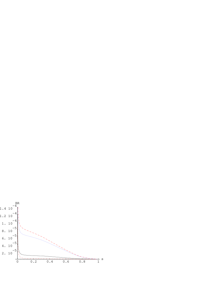
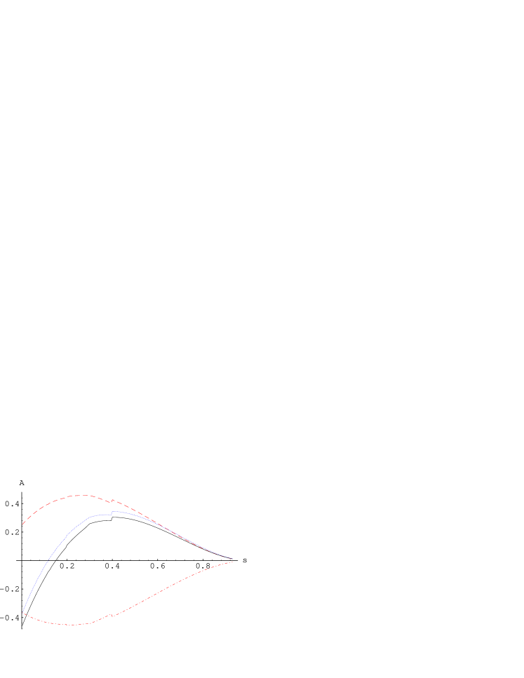
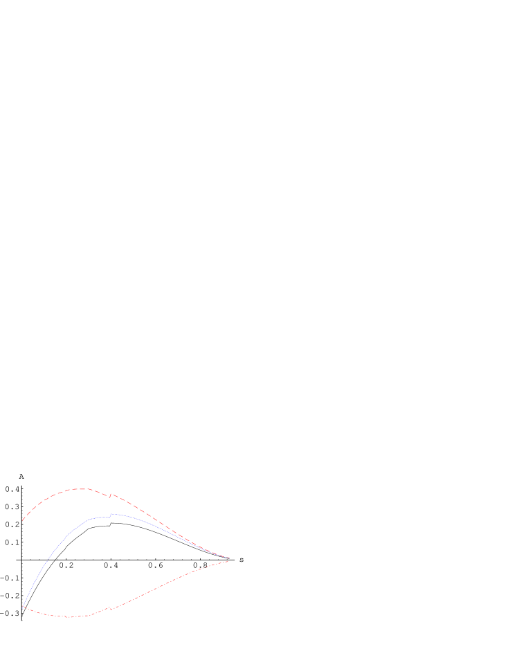
The plots of , and are drawn in figs.5-8. Here both SM and SUSY results are shown. The discontinuity in the plot at corresponds to the point at which we have stopped the corrections . In fact a model independent description of the differential asymmetry in the region beyond the parton model is still lacking. Further the peak wich occur at is due to the perturbative remnant of the resonance.
The integrated BRs and asymmetries for the decays and in the SM case and in the SUSY one (with the above choices of the parameters) are summarized in tab.7. There we computed the total perturbative contributions neglecting the resonances; these occur in the intermediate range of the spectrum ( at 3.1 GeV () and at 3.7 GeV () plus others at higher energies). However it is possible to exclude the resonant regions from the experimental analysis by opportune cuts and to correct the effects of their tails in the remaining part of the spectrum.
The results of tab. 7 must be compared with the experimental best limit which reads [36]
| (47) |
A comment on the CMSSM (Constrained MSSM) prediction for the observables we have computed is now necessary. An analysis on the subject is presented in ref. [14]. In this paper the authors show that the effect of CMSSM on the integrated BRs, considering only contributions to and , varies between a depression up to 10% and an enhancement of few percents relative to the corresponding SM values. The asymmetries get even smaller corrections. On the other hand a direct computation of yields [14]
| (48) |
It is worth noting that comparing the above intervals with the experimentally allowed region obtained via RG evolution at the scale of the limits in eqn. (44) (we use only the SM contribution to ; the inclusion of the MSSM corrections does not change significantly the result)
| (49) |
it is excluded that the CMSSM could drive a positive value for . For what concerns the negative interval of values of we see that it can be accommodated both in the CMSSM and in our framework.
Looking at figs 5-8 and table 7 we see that the differences between SM and SUSY predictions can be remarkable. Moreover a sufficiently precise measure of BRs, s and s can either discriminate between the CMSSM and more general SUSY models or give new constraints on mass insertions. Both these kind of informations can be very useful for model building.


8 Conclusions
In this paper an extensive discussion about SUSY contributions to semileptonic decays , is provided. We see that the interplay between and is fundamental in order to give an estimate of the SUSY relevance in these decays. The two kinds of decays are in fact strongly correlated.
Given the constraints coming from the recent measure of and estimating all possible SUSY effects in the MIA framework we see that SUSY has a chance to strongly enhance or depress semileptonic charmless B-decays. The expected direct measure will give very interesting informations about the SM and its possible extensions.
Acknowledgments
We thank S. Bertolini and E. Nardi for fruitful discussions. I.S. wants to thank SISSA, for support and kind hospitality during the elaboration of the first part of this work and Della Riccia Foundation (Florence, Italy) for partial support. The work of L.S. was supported by the German Bundesministerium für Bildung und Forschung under contract 06 TM 874 and by the DFG project Li 519/2-2. This work was partially supported by INFN and by the TMR–EEC network “Beyond the Standard Model” (contract number ERBFMRX CT960090).
References
- [1] See, for instance, The BaBar Physics Book, SLAC-R-504 and references therein.
- [2] B. Grinstein, M. J. Savage and M. B. Wise Nucl. Phys. B319 (1989) 271.
- [3] G. Buchalla and A. J. Buras, Nucl. Phys. B400 (1993), 225; M. Misiak, Nucl. Phys. B393 (1993) 23, erratum ibid. B439 (1995) 461; A. J. Buras and M. Münz, Phys. Rev. D52 (1995) 186.
- [4] G. Buchalla, A. J. Buras and M. E. Lautenbacher, Rev. Mod. Phys. 68 (1996) 1125.
- [5] N. G. Deshpande, J. Trampetic and K. Panrose, Phys. Rev. D39 (1989) 1461; C. S. Lim, T. Morozumi and A. I. Sanda, Phys. Lett. B218 (1989) 343; A. I. Vainshtein et al., Yad. Fiz. 24 (1976) 820 [Sov. J. Nucl. Phys. 24 (1976) 427]; P. J. O’Donnell and H. K. Tung, Phys. Rev. D43 (1991) 2076.
- [6] A. F. Falk, M. Luke and M. J. Savage, Phys. Rev. D49 (1994) 3367.
- [7] A. Ali, G. Hiller, L. T. Handoko and T. Morozumi, Phys. Rev. D55 (1997) 4105; A. Ali and G. Hiller, Phys. Rev. D58 (1998) 071501 and Phys. Rev. D58 (1998) 074001.
- [8] G. Buchalla and G. Isidori, Nucl. Phys. B525 (1998) 333.
- [9] F. Krüger and L. M. Sehgal, Phys. Lett. B380 (1996) 199; A. Ali, T. Mannel and T. Morozumi, Phys. Rev. B273 (1991) 505; M. R. Ahmadi, Phys. Rev. D53 (1996) 2843; C. D. Lü and D. X. Zhang, Phys. Lett. B397 (1997) 279.
- [10] G. Buchalla, G. Isidori and S. J. Rey, Nucl. Phys. B511 (1998) 594.
- [11] J. W. Chen, G. Rupak and M. J. Savage, Phys. Rev. B410 (1997) 285.
- [12] S. Bertolini, F. Borzumati, A. Masiero and G. Ridolfi, Nucl. Phys. B353 (1991) 591.
- [13] A. Ali, G. F. Giudice and T. Mannel, Z. Phys. C67 (1995) 417; J. Hewett and J. D. Wells, Phys. Rev. D55 (1997) 5549.
- [14] P. Cho, M. Misiak and D. Wyler, Phys. Rev. D54 (1996) 3329.
- [15] T. Goto, Y. Okada, Y. Shimizu and M. Tanaka, Phys. Rev. D55 (1997) 4273; T. Goto, Y. Okada and Y. Shimizu, Phys. Rev. D58 (1998) 094006.
- [16] CLEO Collaboration, CONF98-17, ICHEP98, 1011.
- [17] Y. G. Kim, P. Ko, J. S. Lee, Nucl. Phys. B544 (1999) 64.
- [18] S. Baek and P. Ko, hep-ph/9904283.
- [19] L. J. Hall, V. A. Kostolecki and S. Raby, Nucl. Phys. B267 (1986) 415.
- [20] F. Gabbiani and A. Masiero, Nucl. Phys. B322 (1989) 235.
- [21] J. S. Hagelin, S. Kelley and T. Tanaka, Nucl. Phys. B415 (1994) 293-331; E. Gabrielli, A. Masiero and L. Silvestrini, Phys. Lett. B374 (1996) 80; J. A. Bagger, K. T. Matchev and R. Zhang, Phys. Lett. B412 (1997) 77-85; M. Ciuchini et al., JHEP 10 (1998) 008; R. Contino and I. Scimemi, hep-ph/9809437.
- [22] F. Gabbiani, E. Gabrielli, A. Masiero and L. Silvestrini, Nucl. Phys. B477 (1996) 321.
- [23] J. A. Casas and S. Dimopoulos, Phys. Lett. B387 (1996) 107.
- [24] G. Colangelo and G. Isidori, JHEP 09 (1998) 009.
- [25] N. Cabibbo and L. Maiani, Phys. Lett. B79 (1978) 109; C. S. Kim and A. D. Martin, Phys. Lett. B225 (1989) 186.
- [26] P. Ball and V. M. Braun, Phys. Rev. D49 (1994) 2472; V. Eletsky and E. Shuryak, Phys. Lett. B206 (1992) 191; M. Neubert, Phys. Lett. B322 (1994) 419.
- [27] M. Neubert, Phys. Lett. B389 (1996) 727.
- [28] R. Casalbuoni et al., Phys. Rep. 281 (1997) 145.
- [29] P. Colangelo and P. Santorelli, Phys. Lett. B327 (1994) 123; P. Colangelo, F. De Fazio, P. Santorelli and E. Scrimieri, Phys. Rev. D53 (1996) 3672; P. Colangelo, F. De Fazio, P. Santorelli and E. Scrimieri, Phys. Rev. D57 (1998) 3186.
- [30] V. M. Belyaev, A. Khodjamirian and R. Ruckl, Z. Phys. C60 (1993) 349; P. Ball, JHEP 09 (1998) 005.
- [31] M. Ladisa, G. Nardulli and P. Santorelli, Phys. Lett. B455 (1999) 283.
- [32] A. J. Buras, A. Romanino and L. Silvestrini, Nucl. Phys. B520 (1998) 3.
- [33] C. Caso et al. Eur. Phys. J. C (1998) 1.
- [34] See e.g. A. Kagan and M. Neubert, hep-ph/9805303; A. Czarnecki and W. Marciano, Phys. Rev. Lett. 81 (1998) 277 and refs. therein.
- [35] K. Chetyrkin, M. Misiak and M. Münz, Phys. Lett. B400 (1997) 206-219; Erratum-ibid. B425 (1998) 414.
- [36] S. Glenn et al. (CLEO Collaboration), Phys. Rev. Lett. 80 (1998) 2289.