Hard scattering factorization and light cone hamiltonian approach to diffractive processes

F. Hautmann^a, Z. Kunszt^b and D.E. Soper^c,d

^a Department of Physics, Pennsylvania State University, University Park PA 16802, USA

^b Institute of Theoretical Physics, ETH, CH-8093 Zurich, Switzerland

^c Institute of Theoretical Science, University of Oregon, Eugene OR 97403, USA

^d Theory Division, CERN, CH-1211 Geneva 23, Switzerland

Abstract

We describe diffractive deeply inelastic scattering in terms of diffractive parton distributions. We investigate these distributions in a hamiltonian formulation that emphasizes the spacetime picture of diffraction scattering. For hadronic systems with small transverse size, diffraction occurs predominantly at short distances and the diffractive parton distributions can be studied by perturbative methods. For realistic, large-size systems we discuss the possibility that diffractive parton distributions are controlled essentially by semihard physics at a scale of nonperturbative origin of the order of a GeV. We find that this possibility accounts for two important qualitative aspects of the diffractive data from HERA: the flat behavior in $\beta$ and the delay in the fall-off with $Q^{2}$.

CERN-TH/99-154

ETH-TH/99-09

PSU-TH/207

May 1999

1. Introduction

In hadron-hadron scattering, a substantial fraction of the events are diffractive: one or both of the initial hadrons emerges with small transverse momentum in the final state, having lost only a small fraction of its energy. Assuming that quantum chromodynamics is the theory of the strong interactions, one expects that diffractive scattering is due to the exchange of gluons. Since gluons are pointlike objects, the gluon exchange picture suggests the possibility of hard diffractive scattering, in which exchanged gluons moving in opposite directions participate in a hard process such as jet production, with a transferred-momentum scale much larger than $\Lambda_{\rm{QCD}}$. Similarly, in lepton-hadron scattering it should be possible to have a hard process, deeply inelastic scattering, in which the incoming hadron is diffractively scattered. These possibilities were suggested in 1985 by Ingelman and Schlein [1]. Experimental data from both hadron-hadron [2, 3] and lepton-hadron [4, 5, 6] colliders have confirmed the existence of hard diffractive scattering.

Since hard diffractive scattering contains a hard subprocess, one may ask whether the QCD factorization theorem that holds for inclusive hard scattering works also for diffractive hard scattering. Investigation of this question indicates that factorization does not hold for diffractive hard processes when there are two hadrons in the initial state. In inclusive hard scattering there are contributions from particular final states that would break factorization, but these contributions cancel because of the unitarity of the scattering matrix when one sums over all final states [7]. If only diffractive final states are allowed, this cancellation is spoiled [8, 9]. However, factorization does hold for diffractive deeply inelastic scattering, in which there is only one hadron in the initial state [9, 10, 11]. It is diffractive deeply inelastic scattering that is of concern in this paper.

In diffractive deeply inelastic scattering, one can measure the diffractive structure function $dF_{2}^{\rm diff}(x,Q^{2},x_{\scriptscriptstyle\kern-0.50003ptI\kern-1.25ptP},t)/[dx_{\scriptscriptstyle\kern-0.50003ptI\kern-1.25ptP}\,dt]$, where $Q^{2}$ and $x$ are as usual the photon virtuality and the Bjorken variable of deeply inelastic scattering, $x_{\scriptscriptstyle\kern-0.50003ptI\kern-1.25ptP}$ is the fractional loss of longitudinal momentum by the diffracted hadron, and $t$ is the invariant momentum transfer from the diffracted hadron. This structure function is often called $F_{2}^{D(4)}$. The factorization theorem allows us to write

$${{dF_{2}^{\rm diff}(x,Q^{2},x_{\scriptscriptstyle\kern-0.50003ptI\kern-1.25ptP},t)}\over{dx_{\scriptscriptstyle\kern-0.50003ptI\kern-1.25ptP}\,dt}}\ =\sum_{a}\,\int d\xi\,{df_{a/A}^{\rm diff}(\xi,x_{\scriptscriptstyle\kern-0.50003ptI\kern-1.25ptP},t,\mu)\over dx_{\scriptscriptstyle\kern-0.50003ptI\kern-1.25ptP}\,dt}{\hat{F}}_{a}(x/\xi,Q^{2}/\mu^{2})\hskip 8.5359pt.$$ (1.1)

The function ${\hat{F}}_{a}$ is the hard scattering function, calculable in perturbation theory. It is the same hard scattering function as in inclusive deeply inelastic scattering. The function $df_{a/A}^{\rm{diff}}/[dx_{\scriptscriptstyle\kern-0.50003ptI\kern-1.25ptP}\,dt]$ in Eq. (1.1) is the diffractive parton distribution, containing the long distance physics. It is interpreted as the probability to find a parton of type $a$ in a hadron of type $A$ carrying momentum fraction $\xi$ and, at the same time, to find that the hadron appears in the final state carrying a fraction $1-x_{\scriptscriptstyle\kern-0.50003ptI\kern-1.25ptP}$ of its longitudinal momentum, having been scattered with an invariant momentum transfer $t$. Both the hard scattering function $\hat{F}$ and the diffractive parton distribution functions $df_{a/A}^{\rm diff}/[dx_{\scriptscriptstyle\kern-0.50003ptI\kern-1.25ptP}\,dt]$ depend on a factorization scale $\mu$. The $\mu$ dependence of the distribution functions is given by the usual renormalization group evolution equation,

$${\partial\over{\partial\ln\mu^{2}}}\,{df_{a/A}^{\rm diff}(\xi,x_{\scriptscriptstyle\kern-0.50003ptI\kern-1.25ptP},t,\mu)\over dx_{\scriptscriptstyle\kern-0.50003ptI\kern-1.25ptP}\,dt}=\sum_{a}\,\int d\xi^{\prime}\,K_{aa^{\prime}}(\xi^{\prime},\mu)\,{df_{a^{\prime}/A}^{\rm diff}(\xi/\xi^{\prime},x_{\scriptscriptstyle\kern-0.50003ptI\kern-1.25ptP},t,\mu)\over dx_{\scriptscriptstyle\kern-0.50003ptI\kern-1.25ptP}\,dt}\hskip 8.5359pt,$$ (1.2)

where the kernel $K_{aa^{\prime}}$ has a perturbative expansion in powers of $\alpha_{s}(\mu)$. The diffractive parton distributions are defined as certain matrix elements of quark and gluon field operators, analogously to the definition of the ordinary (inclusive) parton distributions [10]. We will discuss these definitions later in the paper.

Our purpose in this paper is to investigate the diffractive parton distribution functions, expanding on the analysis reported in Ref. [12]. We are interested in the leading behavior of these functions when $x_{\scriptscriptstyle\kern-0.50003ptI\kern-1.25ptP}\ll 1$. In the language of Regge theory, this corresponds to looking in the region where the pomeron is dominant over other Regge poles. Although the evolution equation for the diffractive parton distribution functions is the same as that of the inclusive parton distribution functions, their behavior at a fixed scale $\mu_{0}$ that serves as the starting point for evolution may be very different from the behavior of the inclusive functions. The different phenomenology that characterizes diffractive versus inclusive deeply inelastic scattering depends entirely on this.

Of course, the diffractive parton distributions in a proton at the scale $\mu_{0}$ are not perturbatively calculable. Notice that the problem lies with the large transverse size of the proton. Suppose one had a hadron of a size $1/M$ that is small compared to $1/\Lambda_{\rm{QCD}}$. Then one could compute diffractive parton distributions as a perturbation expansion. In this paper, we first consider diffraction of small-size hadronic systems. We study this in detail. Then, we discuss how the picture of diffraction changes as we let the size increase. This involves nonperturbative dynamics. We explore whether one may extract (at least, qualitative) information on the diffractive parton distributions for a large-size system by supplementing the computation at a much smaller size scale with a hypothesis on the infrared behavior of the diffraction process.

As a simple case of a small-size hadronic system, we consider a diquark system produced by a color-singlet current that couples only to heavy quarks of mass $M\gg\Lambda_{\rm{QCD}}$. This system gets diffracted and acts as a color source with small radius of order $1/M$. In this case, the perturbation expansion for the leading $1/x_{\scriptscriptstyle\kern-0.50003ptI\kern-1.25ptP}\to\infty$ terms in the diffractive parton distributions begins at order $\alpha_{s}^{4}$. Although this is a rather high order of perturbation theory, we find that the result has quite a simple structure and can be expressed in terms of integrals that can be evaluated numerically.

One can view the problem that we address as being that of diffractive deeply inelastic scattering at scale $Q$ from a hadron of size $1/M$ with $Q\ \hbox{\raise 2.0pt\hbox{$>$} \kern-13.0pt\lower 3.0pt\hbox{$\sim$}}\ M$ and $x_{\scriptscriptstyle\kern-0.50003ptI\kern-1.25ptP}\ll 1$. There are two main ingredients in our analysis.

The first ingredient has already been introduced: the factorization formula (1.1). Using factorization, we are led to analyze the diffractive parton distribution functions, which are simpler than $F_{2}^{\rm diff}$. This ingredient is especially important because (as we will see) the diffractive gluon distribution makes an important contribution to $F_{2}^{\rm diff}$, but this contribution is not so easy to analyze systematically without the use of the factorization formula.

The second ingredient is the physical picture that, in a suitable reference frame, the partons that are “measured” in the process are created by the measurement operator outside of the hadron and, much later, interact with the hadron. This picture, called the “aligned jet” model by Bjorken [13], applies when $x_{\scriptscriptstyle\kern-0.50003ptI\kern-1.25ptP}\ll 1$. We will see that it emerges most naturally when one works in configuration space using light cone coordinates

$$x^{\pm}={{x^{0}\pm x^{3}}\over{\sqrt{2}}}\hskip 8.5359pt.$$ (1.3)

The calculation becomes particularly transparent when one uses a hamiltonian formulation in which the theory is quantized on planes of equal $x^{-}$. We will see how this works in Sec. 3.

The plan of the paper is as follows. In Sec. 2 we review the operator definitions for diffractive parton distributions and describe their structure at large $1/x_{\scriptscriptstyle\kern-0.50003ptI\kern-1.25ptP}$. In Sec. 3 we show how to compute these distributions in the light cone hamiltonian formulation of the theory. In Sec. 4 we present general properties and numerical results for the distributions. In Sec. 5 we comment on their evolution and the structure of ultraviolet divergences. In Sec. 6 we discuss the relation of the previous calculations with the phenomenology of diffractive deeply inelastic scattering at HERA. We give conclusions in Sec. 7. In Appendices A-D we give calculational details on certain operator matrix elements, we outline the main steps of the covariant formulation alternative to the one presented in the text, and we collect some integrals.

2. Basic definitions and approximations

In this section, we outline the parts of our analysis that bear on the general structure of the result. We begin with the operator definitions of the diffractive parton distributions. Then we describe how the diffractive parton distributions break into a convolution of a part associated with these operators and a part associated with the wave function of the incoming state.

2.1 Operator definitions

Let us briefly recall the definition of the diffractive parton distributions in terms of matrix elements of bilocal field operators [10]. This is the same definition [14, 15] as for inclusive parton distributions except that one requires that the final state include the diffractively scattered hadron. Let $(p_{A},s_{A})$ and $(p_{\!A^{\prime}},s_{\!A^{\prime}})$ denote the momentum and spin of the incident and the diffracted hadron. Let us adopt the standard notation $\beta x_{\scriptscriptstyle\kern-0.50003ptI\kern-1.25ptP}$ for the hadron momentum fraction carried by the parton. For gluons one has

$${{d\,f_{g/A}^{\rm{diff}}(\beta x_{\scriptscriptstyle\kern-0.50003ptI\kern-1.25ptP},x_{\scriptscriptstyle\kern-0.50003ptI\kern-1.25ptP},t,\mu)}\over{dx_{\scriptscriptstyle\kern-0.50003ptI\kern-1.25ptP}\,dt}}={1\over{16\,\pi^{2}}}\,{1\over 2\pi\beta x_{\scriptscriptstyle\kern-0.50003ptI\kern-1.25ptP}p_{\!A}^{+}}{1\over 2}\sum_{s_{\!A}}\int dy^{-}e^{i\beta x_{\scriptscriptstyle\kern-0.50003ptI\kern-1.25ptP}p_{\!A}^{+}y^{-}}\sum_{X,s_{\!A^{\prime}}}$$

$$\hskip 28.45274pt\times\langle p_{\!A},s_{\!A}|\widetilde{F}_{a}(0)^{+j}|p_{\!A^{\prime}},s_{\!A^{\prime}};X\rangle\langle p_{\!A^{\prime}},s_{\!A^{\prime}};X|\widetilde{F}_{a}(0,y^{-},{\bf 0})^{+j}|p_{\!A},s_{\!A}\rangle\hskip 5.69046pt,$$ (2.1)

where there is an implicit sum over $j=1,2$ and where $\widetilde{F}_{a}(0,y^{-},{\bf 0})^{+\nu}$ is the field strength operator modified by multiplication by an exponential of a line integral of the vector potential:

$$\widetilde{F}_{a}(y)^{+j}=E(y)_{ab}F_{b}(y)^{+j}\hskip 5.69046pt,$$ (2.2)

where

$$E(y)={\cal P}\exp\left(-ig\int_{y^{-}}^{\infty}dx^{-}\,A_{c}^{+}(y^{+},x^{-},{\bf y})\,t_{c}\right)\hskip 8.5359pt.$$ (2.3)

The symbol ${\cal P}$ denotes path ordering of the exponential. The matrices $t_{c}$ in Eq. (2.3) are the generators of the adjoint representation of SU(3), $(t_{c})_{bd}=-if_{cbd}$.

The field operators in Eq. (S0.Ex1) are evaluated at points separated by lightlike distances. There are ultraviolet divergences from the operator products. It is understood that these are renormalized at the scale $\mu$ using the $\overline{\rm MS}$ prescription.

For purposes of computations, there is a more useful way [14] to write $\widetilde{F}^{+j}$. Starting with

$$\widetilde{F}_{a}(y)^{+j}=E(y)_{ab}\left[\partial^{+}A_{b}(y)^{j}-\partial^{j}A_{b}(y)^{+}+igA_{c}(y)^{+}A_{d}(y)^{j}\ (t_{c})_{bd}\right]\hskip 8.5359pt,$$ (2.4)

we have

$$\widetilde{F}_{a}(y)^{+j} = \partial^{+}(E(y)_{ab}A_{b}(y)^{j})-igE(y)_{ab}A_{c}(y)^{+}(t_{c})_{bd}\ A_{d}(y)^{j}$$ (2.5)

$$-E(y)_{ab}\partial^{j}A_{b}(y)^{+}+igE(y)_{ab}A_{c}(y)^{+}A_{d}(y)^{j}\ (t_{c})_{bd}\hskip 8.5359pt.$$

The second and fourth terms cancel. Furthermore, inside the integration in Eq. (S0.Ex1), $\partial^{+}=\partial/\partial x^{-}$ becomes $-i\beta x_{\scriptscriptstyle\kern-0.50003ptI\kern-1.25ptP}p_{A}^{+}$:

$$\widetilde{F}_{a}(y)^{+j}\to E(y)_{ab}[-i\beta x_{\scriptscriptstyle\kern-0.50003ptI\kern-1.25ptP}p_{A}^{+}\ A_{b}(y)^{j}-\partial^{j}A_{b}(y)^{+}]\hskip 8.5359pt.$$ (2.6)

This form is useful because it does not have an $A\times A$ term and it does not have a $\partial/\partial x^{-}$. (In the complex conjugate matrix element in Eq. (S0.Ex1), the $-i\beta x_{\scriptscriptstyle\kern-0.50003ptI\kern-1.25ptP}p_{A}^{+}$ becomes $+i\beta x_{\scriptscriptstyle\kern-0.50003ptI\kern-1.25ptP}p_{A}^{+}$.)

For quarks of type $j$ one has

$${{d\,f_{j/A}^{\rm{diff}}(\beta x_{\scriptscriptstyle\kern-0.50003ptI\kern-1.25ptP},x_{\scriptscriptstyle\kern-0.50003ptI\kern-1.25ptP},t,\mu)}\over{dx_{\scriptscriptstyle\kern-0.50003ptI\kern-1.25ptP}\,dt}}={1\over{16\,\pi^{2}}}\,{1\over 2\pi\beta x_{\scriptscriptstyle\kern-0.50003ptI\kern-1.25ptP}p_{A}^{+}}{1\over 2}\sum_{s_{\!A}}\int dy^{-}e^{i\beta x_{\scriptscriptstyle\kern-0.50003ptI\kern-1.25ptP}p_{\!A}^{+}y^{-}}\sum_{X,s_{\!A^{\prime}}}$$

$$\hskip 28.45274pt\times{\beta x_{\scriptscriptstyle\kern-0.50003ptI\kern-1.25ptP}p_{A}^{+}\over 2}\langle p_{\!A},s_{\!A}|\widetilde{\overline{\Psi}}(0)|p_{\!A^{\prime}},s_{\!A^{\prime}};X\rangle\gamma^{+}\langle p_{\!A^{\prime}},s_{\!A^{\prime}};X|{\widetilde{\Psi}}(0,y^{-},{\bf 0})|p_{\!A},s_{\!A}\rangle\hskip 5.69046pt,$$ (2.7)

where

$$\widetilde{\Psi}_{j}(y)=E(y)\Psi_{j}(y)\hskip 5.69046pt.$$ (2.8)

Here $E(y)$ is given by Eq. (2.3) with, now, the matrices $t_{c}$ being the generators of the fundamental representation of SU(3).

2.2 General structure at large $1/x_{\scriptscriptstyle\kern-0.60004ptI\kern-1.5ptP}$

As discussed in Sec. 1, the scattering process we consider is initiated by a color-singlet current. We specialize the definitions of the previous subsection to the case in which the incident hadron $A$ is a special photon that couples to a heavy quark-antiquark pair of mass $M$. This pair couples again to the diffractively scattered photon in the final state.

In the discussion that follows, we use the same method for the diffractive quark distribution and the diffractive gluon distribution. For the sake of definiteness, we present the discussion in the case of the diffractive gluon distribution. At the end of Sec. 3 we will give the extension of the results to the case of the quark.

We consider the limiting $1/x_{\scriptscriptstyle\kern-0.50003ptI\kern-1.25ptP}\to\infty$ behavior of graphs for the diffractive gluon distribution. We shall find contributions proportional to $x_{\scriptscriptstyle\kern-0.50003ptI\kern-1.25ptP}^{-2}$ at fixed $\beta$. At higher orders in perturbation theory, the $x_{\scriptscriptstyle\kern-0.50003ptI\kern-1.25ptP}^{-2}$ would be supplemented by logarithms of $x_{\scriptscriptstyle\kern-0.50003ptI\kern-1.25ptP}$. In this paper we will limit ourselves to considering the graphs at the lowest order of perturbation theory for which $x_{\scriptscriptstyle\kern-0.50003ptI\kern-1.25ptP}^{-2}$ behavior emerges.

What are the lowest order graphs that can give $x_{\scriptscriptstyle\kern-0.50003ptI\kern-1.25ptP}^{-2}$ behavior? Note that there must be at least one gluon in the final state in order to balance the color of the operator that measures the gluon distribution. We find that with exactly one gluon in the final state there are $x_{\scriptscriptstyle\kern-0.50003ptI\kern-1.25ptP}^{-2}$ contributions at order $\alpha_{s}^{4}$. An example of a contributing graph is shown in Fig. 1. Note that there are graphs that contribute to the diffractive gluon distribution at one lower order of perturbation theory, but they yield fewer powers of $1/x_{\scriptscriptstyle\kern-0.50003ptI\kern-1.25ptP}$. Thus we consider $\alpha_{s}^{4}$ contributions.

We write the hadron momenta as

$$p_{A}^{\mu} = (p_{A}^{+},0,{\bf 0})$$

$$p_{A^{\prime}}^{\mu} = ((1-x_{\scriptscriptstyle\kern-0.50003ptI\kern-1.25ptP})p_{A}^{+},{{\bf q}^{2}\over 2(1-x_{\scriptscriptstyle\kern-0.50003ptI\kern-1.25ptP})p_{A}^{+}},-{\bf q)}\hskip 8.5359pt.$$ (2.9)

Thus the momentum transfer is

$$q^{\mu}\equiv p_{A}^{\mu}-p_{A^{\prime}}^{\mu}=(x_{\scriptscriptstyle\kern-0.50003ptI\kern-1.25ptP}p_{A}^{+},-{{\bf q}^{2}\over 2(1-x_{\scriptscriptstyle\kern-0.50003ptI\kern-1.25ptP})p_{A}^{+}},{\bf q)}\hskip 8.5359pt.$$ (2.10)

The invariant momentum transfer is $t\equiv q_{\mu}q^{\mu}=-{\bf q}^{2}/(1-x_{\scriptscriptstyle\kern-0.50003ptI\kern-1.25ptP})$. Since we are interested in the $x_{\scriptscriptstyle\kern-0.50003ptI\kern-1.25ptP}\to 0$ limit, we use the approximation $t\approx-{\bf q}^{2}$. We suppose that ${\bf q}^{2}\ \hbox{\raise 2.0pt\hbox{$<$} \kern-13.0pt\lower 3.0pt\hbox{$\sim$}}\ M^{2}$.

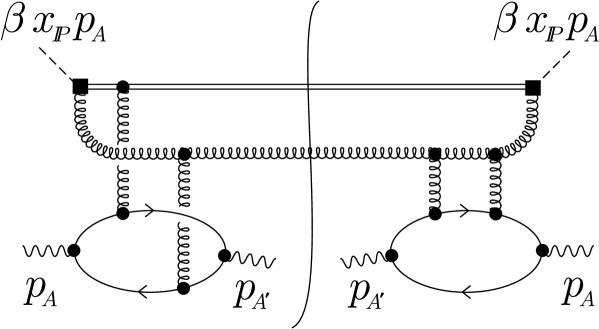
Figure 1: A particular graph that contributes to the diffractive gluon distribution.

It is useful to work in a frame in which $p_{A}^{+}\sim M$, so that the initial hadron is approximately at rest.

We have a final state particle with momentum

$$k^{\mu}=({{\bf k}^{2}\over 2k^{-}},k^{-},{\bf k})\hskip 8.5359pt.$$ (2.11)

Since plus momentum $q^{+}=x_{\scriptscriptstyle\kern-0.50003ptI\kern-1.25ptP}p_{A}^{+}$ is delivered from the scattered hadron and plus momentum $\beta x_{\scriptscriptstyle\kern-0.50003ptI\kern-1.25ptP}p_{A}^{+}$ is removed by the measurement operator, plus momentum

$${{\bf k}^{2}\over 2k^{-}}=(1-\beta)x_{\scriptscriptstyle\kern-0.50003ptI\kern-1.25ptP}p_{A}^{+}$$ (2.12)

remains for the final state particle. Let us assume (as we will find, self-consistently, in this calculation) that there are no important integration regions with ${\bf k}^{2}\ll M^{2}$ or with ${\bf k}^{2}\gg M^{2}$. That is, ${\bf k}^{2}\sim M^{2}$ in the integration regions that give leading contributions. Then $k^{-}$ must be large, $k^{-}\ \hbox{\raise 2.0pt\hbox{$>$} \kern-13.0pt\lower 3.0pt\hbox{$\sim$}}\ M/x_{\scriptscriptstyle\kern-0.50003ptI\kern-1.25ptP}$. The observation that the final state parton has large minus momentum is crucial to the calculation.

Our analysis is simplified if we choose a physical gauge. Since the gluon in the final state has large minus momentum, it is natural [16] to use the null-plane gauge $A^{-}=0$. (We make a few remarks on the calculation in Feynman gauge in Appendix C.)

We have seen that the final state hadron has a minus component of momentum of order $M$ while the final state parton has minus momentum of order $M/x_{\scriptscriptstyle\kern-0.50003ptI\kern-1.25ptP}\gg M$. For the virtual particles, we divide the integration over minus momenta into regions $\ell^{-}\sim M$ and $\ell^{-}\gg M$. In a general Feynman graph, it is far from easy to make this division, but at order $\alpha_{s}^{4}$ the situation turns out to be quite simple.

In particular, the heavy quarks in our model hadron must have $\ell^{-}\sim M$. In order to leave the hadron in a color singlet state, two gluons (at least) must attach to the heavy quarks. In order that the intermediate heavy quark lines not be far off shell, the minus momentum delivered by each of these gluons must not be large. Finally, the only sink for the large minus momentum carried by the final state gluon is the vertex representing the measurement operator $\widetilde{F}^{\nu+}$, which can absorb large $\ell^{-}$ since it is evaluated at a fixed value of plus position, $x^{+}=0$. With a little thought, one realizes that all of the remaining internal propagator lines must carry large minus momentum.

We are thus led to the picture shown in Fig. 2. In the lower subgraph, all loop momenta have $\ell^{-}\sim M$. In the upper subgraph, all loop momenta have $\ell^{-}\gg M$. Two gluon lines with $\ell^{-}\sim M$ communicate between the two subgraphs. An example of a graph that contributes to Fig. 2 is shown in Fig. 1.

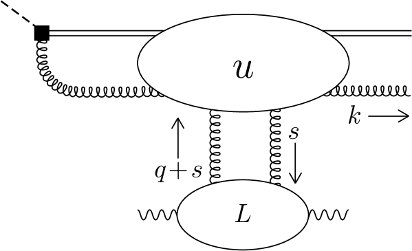
Figure 2: Structure of the diffractive gluon distribution. In the amplitude, two gluons are exchanged, one gluon is absorbed by the measurement operator, and one gluon is emitted into the final state. The subgraphs $u$ and $L$ are evaluated at lowest order of perturbation theory.

The definition (S0.Ex1) together with the structure represented by Fig. 2 lead to the following expression for the diffractive gluon distribution:

$${{df_{g/A}^{\rm{diff}}(\beta x_{\scriptscriptstyle\kern-0.50003ptI\kern-1.25ptP},x_{\scriptscriptstyle\kern-0.50003ptI\kern-1.25ptP},{\mbox{\bf q}}^{2},M)}\over{dx_{\scriptscriptstyle\kern-0.50003ptI\kern-1.25ptP}\,dt}} = {1\over{16\pi^{2}}}\,{1\over 2\pi\beta x_{\scriptscriptstyle\kern-0.50003ptI\kern-1.25ptP}p_{A}^{+}}\,{1\over 2}\,\sum_{\varepsilon\,\varepsilon^{\prime}}\,\int\!{d^{4}s\over(2\pi)^{4}}\,\int\!{d^{4}s^{\prime}\over(2\pi)^{4}}\,\int\!{d^{2}{\bf k}\,dk^{+}\over(2\pi)^{3}2k^{+}}\,$$ (2.13)

$$\times{\rm Tr}\left\{u_{0}^{\dagger}(k,q,s^{\prime})^{\alpha\beta}_{ab}\ u_{0}(k,q,s)^{\gamma\delta}_{cd}\right\}(2\pi)\delta(k^{+}-(1-\beta)x_{\scriptscriptstyle\kern-0.50003ptI\kern-1.25ptP}p_{A}^{+})$$

$$\times{1\over 4}\ {-iD(s^{\prime})_{\alpha\mu}\over s^{\prime 2}-i\epsilon}\ {-iD(q+s^{\prime})_{\beta\nu}\over(q+s^{\prime})^{2}-i\epsilon}\ {iD(s)_{\gamma\rho}\over s^{2}+i\epsilon}\ {iD(q+s)_{\delta\sigma}\over(q+s)^{2}+i\epsilon}\$$

$$\times L_{0}(q,s^{\prime},\varepsilon,\varepsilon^{\prime})^{\mu\nu}_{ab}\ L_{0}(q,s,\varepsilon,\varepsilon^{\prime})^{\rho\sigma}_{cd}\ \hskip 8.5359pt.$$

Here the $(2\pi)\delta(k^{+}-(1-\beta)x_{\scriptscriptstyle\kern-0.50003ptI\kern-1.25ptP}p_{A}^{+})$ results from performing the integration over $y^{-}$ in Eq. (S0.Ex1). We note immediately that the integration over the plus momentum of the final state gluon gives

$$\int{dk^{+}\over(2\pi)2k^{+}}\ (2\pi)\delta(k^{+}-(1-\beta)x_{\scriptscriptstyle\kern-0.50003ptI\kern-1.25ptP}p_{A}^{+})={1\over 2(1-\beta)x_{\scriptscriptstyle\kern-0.50003ptI\kern-1.25ptP}p_{A}^{+}}\hskip 8.5359pt.$$ (2.14)

The functions $u_{0}$ and $L_{0}$ are the amputated Green functions represented in Fig. 2. The subscripts 0 distinguish these functions from simpler functions $u$ and $L$ that are defined below in terms of $u_{0}$ and $L_{0}$ and appear in the final formula (2.20) for the diffractive gluon distribution. The function $u_{0}$ carries two transverse vector indices that are not shown. One is the index $j$ carried by the operator $F_{a}^{+j}$ in Eq. (S0.Ex1), the other is the transverse polarization index of the final state gluon. It also carries two color indices: the color index $a$ of $F_{a}^{+j}$ and the color index of the final state gluon. The notation ${\rm Tr}\{u_{0}^{\dagger}u_{0}\}$ denotes a summation over these polarization and color indices. The indices carried by $u_{0}$ that are displayed are the color and polarization indices for the exchanged gluons. The counting factor 1/4 associated with the gluon exchange accounts for the two ways for attaching the labels $s^{\prime}$ and $q+s^{\prime}$ to the two gluons to the right of the final state cut and the two ways for attaching the labels $s$ and $q+s$ to the two gluons to the left of the final state cut. The notation $iD(\ell)_{\mu\nu}/[\ell^{2}+i\epsilon]$ denotes the propagator of a gluon in null-plane gauge. The Green functions $L_{0}$ depend on the transverse polarization vectors $\varepsilon$ and $\varepsilon^{\prime}$ of the initial and final state photons, respectively. There is a sum over the two choices for each of these polarizations.

We can now make a number of approximations that simplify Eq. (2.13). These approximations will be discussed again in the following section, but we outline them here in order to exhibit their effect on the overall structure of Eq. (2.13).

First, consider the momenta $s$, $q-s$, $s^{\prime}$, and $q+s^{\prime}$ of the exchanged gluons. We have taken $|{\bf q}|\ \hbox{\raise 2.0pt\hbox{$<$} \kern-13.0pt\lower 3.0pt\hbox{$\sim$}}\ M$. Let us assume that (as we will find, self-consistently, in this calculation) that $|{\bf s}|$ and $|{\bf s}^{\prime}|$ are of order $M$ in the integration region that gives the leading contributions. Now $s^{+}$ must be of order $M^{2}/k^{-}$, where $k^{-}$ is the minus momentum of the final state gluon, in order that the gluons in the upper subgraph are not too far off shell. As we have just seen, $k^{-}\sim M/x_{\scriptscriptstyle\kern-0.50003ptI\kern-1.25ptP}$, so $s^{+}\sim x_{\scriptscriptstyle\kern-0.50003ptI\kern-1.25ptP}M$. On the other hand, $s^{-}$ must be of order $M^{2}/p_{A}^{+}\sim M$ in order that the partons in the lower subgraph are not too far off shell. Thus $s^{+}s^{-}\sim x_{\scriptscriptstyle\kern-0.50003ptI\kern-1.25ptP}M^{2}\ll{\bf s}^{2}$. For this reason, the propagator for the exchanged gluon with momentum $s$ is $iD_{\gamma\rho}/s_{\mu}s^{\mu}\approx-iD_{\gamma\rho}/{\bf s}^{2}$. A similar power counting shows that only the transverse part of the momentum in each of the other exchanged gluon propagators contributes in the $1/x_{\scriptscriptstyle\kern-0.50003ptI\kern-1.25ptP}\to\infty$ limit.

Second, $s^{+}$, $s^{\prime+}$ and $q^{+}$, being of order $x_{\scriptscriptstyle\kern-0.50003ptI\kern-1.25ptP}M$, are negligible compared to the plus momenta in the subgraphs $L_{0}$. Thus we replace $s^{+}$, $s^{\prime+}$ and $q^{+}$ by 0 in the subgraphs $L_{0}$. Then the integrations over $s^{+}$ and $s^{\prime+}$ can be associated with the upper subgraphs $u_{0}$. Similarly, $s^{-}$, $s^{\prime-}$, and $q^{-}$, being of order $M$, are negligible compared to the minus momenta in the subgraphs $u_{0}$, which are of order $M/x_{\scriptscriptstyle\kern-0.50003ptI\kern-1.25ptP}$. Thus we replace $s^{-}$, $s^{\prime-}$, and $q^{-}$ by 0 in the subgraphs $u$. Then the integrations over $s^{-}$ and $s^{\prime-}$ can be associated with the lower subgraphs $L_{0}$.

Third, the lower subgraphs in Fig. 2 are proportional to color matrices ${\rm Tr}[t_{a}t_{b}]={\scriptstyle{1\over 2}}\delta_{ab}$. Thus we can replace

$$L_{0}(q,s,\varepsilon,\varepsilon^{\prime})^{\rho\sigma}_{cd}\to\delta_{cd}\ {L_{0}(q,s,\varepsilon,\varepsilon^{\prime})^{\rho\sigma}_{ee}\over N_{c}^{2}-1}\hskip 8.5359pt.$$ (2.15)

Fourth, we will find that in the end only the $g_{\mu\nu}$ parts of the propagators of the exchanged gluons count. Then the Lorentz index structure in Fig. 2 is $u_{0}^{\gamma\delta}L_{0\gamma\delta}$. Since the partons in the upper subgraphs have very large minus momenta, this becomes approximately $u_{0}^{--}L_{0}^{++}$.

With these changes, Eq. (2.13) becomes

$${{df_{g/A}^{\rm{diff}}(\beta x_{\scriptscriptstyle\kern-0.50003ptI\kern-1.25ptP},x_{\scriptscriptstyle\kern-0.50003ptI\kern-1.25ptP},{\mbox{\bf q}}^{2},M)}\over{dx_{\scriptscriptstyle\kern-0.50003ptI\kern-1.25ptP}\,dt}} = {1\over{64\pi^{2}}}\,{1\over 4\pi\beta(1-\beta)x_{\scriptscriptstyle\kern-0.50003ptI\kern-1.25ptP}^{2}(p_{A}^{+})^{2}}\,{1\over 2}\,\sum_{\varepsilon\,\varepsilon^{\prime}}\,\int\!{d^{2}{\bf s}\over(2\pi)^{2}}\,\int\!{d^{2}{\bf s}^{\prime}\over(2\pi)^{2}}\,\int\!{d^{2}{\bf k}\over(2\pi)^{2}}\,$$ (2.16)

$$\times{\rm Tr}\left\{\left(\int\!{ds^{\prime+}\over 2\pi}\,u_{0}^{\dagger}(k,q,s^{\prime})^{--}_{aa}\right)\left(\int\!{ds^{+}\over 2\pi}u_{0}(k,q,s)^{--}_{cc}\right)\right\}$$

$$\times{1\over{\bf s}^{2}}\ {1\over({\bf q}+{\bf s})^{2}}\ {1\over{\bf s}^{\prime 2}}\ {1\over({\bf q}+{\bf s}^{\prime})^{2}}\$$

$$\times\left(\int\!{ds^{\prime-}\over 2\pi}\,{L_{0}(q,s^{\prime},\varepsilon,\varepsilon^{\prime})_{bb}^{++}\over N_{c}^{2}-1}\right)\left(\int\!{ds^{-}\over 2\pi}\,{L_{0}(q,s,\varepsilon,\varepsilon^{\prime})_{dd}^{++}\over N_{c}^{2}-1}\right).$$

Let us define simplified functions $L$ and $u$ by

$$\int\!{ds^{-}\over 2\pi}\,{L_{0}(q,s,\varepsilon,\varepsilon^{\prime})_{bb}^{++}\over N_{c}^{2}-1}=p_{A}^{+}\ L({\bf q},{\bf s},\varepsilon,\varepsilon^{\prime})$$ (2.17)

and

$$\int\!{ds^{+}\over 2\pi}\ u_{0}(k,q,s)^{--}_{aa}={{1\kern-2.70004pt{\rm I}}\,}\,C_{A}\,g_{s}^{2}\,u(\beta,{\bf k},{\bf q},{\bf s})\hskip 8.5359pt,$$ (2.18)

where ${1\kern-2.70004pt{\rm I}}\,$ is a unit matrix in color space. We insert these definitions into Eq. (2.16) and use

$${\rm Tr}\,{1\kern-2.70004pt{\rm I}}\,=N_{c}^{2}-1\hskip 8.5359pt.$$ (2.19)

This leaves a factor ${\rm Tr}\{u^{\dagger}u\}$ in which the trace is now over transverse polarization indices but not color.

These changes give

$${{df_{g/A}^{\rm{diff}}(\beta x_{\scriptscriptstyle\kern-0.50003ptI\kern-1.25ptP},x_{\scriptscriptstyle\kern-0.50003ptI\kern-1.25ptP},{\mbox{\bf q}}^{2},M)}\over{dx_{\scriptscriptstyle\kern-0.50003ptI\kern-1.25ptP}\,dt}} = {1\over{64\pi^{2}}}\,{C_{A}^{2}(N_{c}^{2}-1)g_{s}^{4}\over 4\pi\beta(1-\beta)x_{\scriptscriptstyle\kern-0.50003ptI\kern-1.25ptP}^{2}}\,{1\over 2}\,\sum_{\varepsilon\,\varepsilon^{\prime}}\,\int\!{d^{2}{\bf s}\over(2\pi)^{2}}\,\int\!{d^{2}{\bf s}^{\prime}\over(2\pi)^{2}}\,\int\!{d^{2}{\bf k}\over(2\pi)^{2}}\,$$ (2.20)

$$\times{\rm Tr}\left\{u^{\dagger}(\beta,{\bf k},{\bf q},{\bf s}^{\prime})\,u(\beta,{\bf k},{\bf q},{\bf s})\right\}$$

$$\times{1\over{\bf s}^{2}}\ {1\over({\bf q}+{\bf s})^{2}}\ {1\over{\bf s}^{\prime 2}}\ {1\over({\bf q}+{\bf s}^{\prime})^{2}}\$$

$$\times L({\bf q},{\bf s}^{\prime},\varepsilon,\varepsilon^{\prime})\,L({\bf q},{\bf s},\varepsilon,\varepsilon^{\prime})\hskip 8.5359pt.$$

This formula gives the basic structure of the answer for the matrix element (S0.Ex1). We will now examine this in detail.

3. Diffractive parton distributions and null-plane field theory

In this section, we use the formulation of QCD quantized on planes of equal light cone coordinates to analyze the structure depicted in Fig. 2. In doing so, we will derive explicit expressions for the subgraphs $u$ and $L$. This style of analysis is perhaps less familiar than the approach using covariant Feynman graphs in Feynman gauge, but it expresses the physics of the process in configuration space in a more transparent fashion. For those readers who prefer a standard covariant calculation, we present some of the essential steps in such a calculation in Appendix C. We carry out the calculation of this section for the specific case of the diffractive gluon distribution. Then, in Sec. 3.4, we assemble the complete result for both the gluon and quark distributions.

3.1 The upper subgraph

Consider the function $u(\beta,{\bf k},{\bf q},{\bf s})$ that appears in Eq. (2.20) and is represented by the upper subgraph in Fig. 2. The partons in $u$ move with very large minus momentum through the gluon field that accompanies the heavy quark state that is approximately at rest. Our analysis is designed to draw the consequences of this, concentrating on the development of the states in space and time.

External field to represent the exchanged gluons

It is convenient to replace the gluons coming from the lower subgraph by an external color field ${\cal A}^{\mu}(x)$. We thus consider the matrix element

$${\cal M}=\int dy^{-}e^{i\beta x_{\scriptscriptstyle\kern-0.50003ptI\kern-1.25ptP}p_{A}^{+}y^{-}}\langle k,s|\widetilde{F}_{a}(0,y^{-},{\bf 0})^{+j}|0\rangle_{\cal A}\hskip 5.69046pt.$$ (3.1)

Here $\widetilde{F}^{+j}$ is the measurement operator (2.6) for the gluon distribution function and $k,s$ are the momentum and spin of the final state gluon. The matrix element is evaluated in the presence of an external color field $\cal A$. We expand ${\cal M}$ in perturbation theory and extract the term ${\cal M}_{0,2}$ proportional to two powers of $g_{s}{\cal A}$ and zero additional powers of $g_{s}$. The coefficient in this term is the Green function $u_{0}$ in Eq. (2.13):

$${\cal M}_{0,2}={1\over 2}\int\!{d^{4}s\over(2\pi)^{4}}\int\!{d^{4}q\over(2\pi)^{4}}\ \widetilde{\cal A}_{\gamma}^{c}(-s)\,\widetilde{\cal A}_{\delta}^{d}(q+s)\,2\pi\delta(q^{+}-x_{\scriptscriptstyle\kern-0.50003ptI\kern-1.25ptP}p_{A}^{+})\,u_{0}(k,q,s)^{\gamma\delta}_{cd}\hskip 5.69046pt.$$ (3.2)

Here $\widetilde{\cal A}$ is the Fourier transform of $\cal A$:

$$\tilde{\cal A}_{a}^{\mu}(k)=\int dx\ e^{ik\cdot x}{\cal A}_{a}^{\mu}(x)\hskip 5.69046pt.$$ (3.3)

Since $\cal A$ represents the gluons exchanged with the lower state and these gluons are in a color singlet state (cf. Eq. (2.15)), we will replace

$$\widetilde{\cal A}_{\gamma}^{c}(-s)\,\widetilde{\cal A}_{\delta}^{d}(q+s)\,\to\delta_{cd}\ {1\over N_{C}^{2}-1}\,\widetilde{\cal A}_{\gamma}^{e}(-s)\,\widetilde{\cal A}_{\delta}^{e}(q+s)\,\hskip 5.69046pt.$$ (3.4)

After making this replacement, the arguments that led to Eq. (2.16) lead us to anticipate that ${\cal M}_{0,2}$ becomes much simpler in the $1/x_{\scriptscriptstyle\kern-0.50003ptI\kern-1.25ptP}\to\infty$ limit, taking the form

$${\cal M}_{0,2} \approx {1\over 2}\int\!{d^{2}{\bf s}\over(2\pi)^{2}}\int\!{d^{2}{\bf q}\over(2\pi)^{2}}\int\!{ds^{-}\over 2\pi}\int\!{dq^{-}\over 2\pi}{1\over N_{c}^{2}-1}\ \widetilde{\cal A}^{c+}(0,-s^{-},-{\bf s})\,\widetilde{\cal A}^{c+}(0,q^{-}+s^{-},{\bf q}+{\bf s})\,$$ (3.5)

$$\times\int\!{ds^{+}\over 2\pi}\ u_{0}(k;x_{\scriptscriptstyle\kern-0.50003ptI\kern-1.25ptP}p_{A}^{+},0,{\bf q};s^{+},0,{\bf s})^{--}_{aa}\hskip 5.69046pt.$$

Using Eq. (2.18), we identify the function $u$ that appears in the final formula (2.20) for the diffractive gluon distribution. Thus

$${\cal M}_{0,2} \approx {1\over 2}\int\!{d^{2}{\bf s}\over(2\pi)^{2}}\int\!{d^{2}{\bf q}\over(2\pi)^{2}}\int\!{ds^{-}\over 2\pi}\int\!{dq^{-}\over 2\pi}{1\over N_{c}^{2}-1}\ \widetilde{\cal A}^{c+}(0,-s^{-},-{\bf s})\,\widetilde{\cal A}^{c+}(0,q^{-}+s^{-},{\bf q}+{\bf s})\,$$ (3.6)

$$\times{{1\kern-2.70004pt{\rm I}}\,}\,C_{A}\,g_{s}^{2}\,u(\beta,{\bf k},{\bf q},{\bf s})\hskip 5.69046pt.$$

where ${1\kern-2.70004pt{\rm I}}\,$ is a unit matrix in color space. Our aim in this section is to calculate ${\cal M}_{0,2}$ in the $1/x_{\scriptscriptstyle\kern-0.50003ptI\kern-1.25ptP}\to\infty$ limit, then to use Eq. (3.6) to extract $u(\beta,{\bf k},{\bf q},{\bf s})$.

In order to better illustrate the physical principles involved and to give some indication of how the present calculation would work at higher orders, it is useful to generalize the problem that we attack. Let us therefore consider a matrix element

$${\cal M}=\int dy^{-}e^{i\beta x_{\scriptscriptstyle\kern-0.50003ptI\kern-1.25ptP}p_{A}^{+}y^{-}}\langle k_{1},s_{1},\dots,k_{N},s_{N}|\widetilde{F}_{a}(0,y^{-},{\bf 0})^{+j}|0\rangle_{\cal A}\hskip 5.69046pt.$$ (3.7)

Here $k_{i},s_{i}$ are the momenta and spins of one or possibly more final state partons, with $k_{i}^{-}\sim M/x_{\scriptscriptstyle\kern-0.50003ptI\kern-1.25ptP}$. The matrix element is evaluated in full QCD in the presence of an external color field $\cal A$ considered at all orders of perturbation theory. As $x_{\scriptscriptstyle\kern-0.50003ptI\kern-1.25ptP}\to 0$, the momenta $k_{i}^{-}$ become large. On the other hand, the external field $\cal A$ stays fixed. That is to say, the minus momenta of the quantum particles become large while the minus momenta of the gluons in the field produced by the diffracted hadron stay of order $M$.

The eikonal line

The operator $\widetilde{F}^{+j}$ in Eq. (2.6) contains the exponential of a line integral of the color vector potential, which now includes both the quantum potential $A$ and the external potential ${\cal A}$,

$$E(0,y^{-},{\bf 0})=\exp\left(-ig\int_{y^{-}}^{\infty}dx^{-}[A_{c}^{+}(0,x^{-},{\bf 0})+{\cal A}_{c}^{+}(0,x^{-},{\bf 0})]t_{c}\right)\hskip 5.69046pt.$$ (3.8)

This eikonal line operator produces the same effect as if there were a special color octet particle, ${\cal E}$, with a propagator

$${i\over\ell^{+}+i\epsilon}$$ (3.9)

and an interaction vertex with the color field

$$-igt_{c}n^{\mu}$$ (3.10)

with $n\cdot\epsilon=\epsilon^{+}$. We can build such a particle into the theory. Let the particle be created with an operator $Q_{a}^{\dagger}(y^{-})$ and destroyed with an operator $Q_{a}(y^{-})$. The commutation relation is $[Q_{a}(y^{-}),Q_{b}^{\dagger}(y^{-})]=\delta_{ab}$. The action

$$\int_{-\infty}^{+\infty}\!dx^{-}\ Q_{b}^{\dagger}(x^{-})\left[i{d\over dx^{-}}\delta_{ba}-g[A_{c}^{+}(0,x^{-},{\bf 0})+{\cal A}_{c}^{+}(0,x^{-},{\bf 0})](t_{c})_{ba}\right]Q_{a}(x^{-})$$ (3.11)

will produce the desired propagator and vertices. We need a notation for the states. We use $Q_{b}^{\dagger}(0)|0\rangle=|{\cal E},b\rangle$ and

$$Q_{b}^{\dagger}(0)|k_{1},s_{1},\dots,k_{N},s_{N}\rangle=|k_{1},s_{1},\dots,k_{N},s_{N},{\cal E},b\rangle\hskip 5.69046pt.$$ (3.12)

Thus we can replace the operator $\widetilde{F}^{+j}$ by

$$Q^{\dagger}(y^{-})_{a}{\cal O}_{a}^{j}(0,y^{-},{\bf 0})\hskip 5.69046pt,$$ (3.13)

where, using Eq. (2.6),

$${\cal O}_{a}^{j}(y)=-i\beta x_{\scriptscriptstyle\kern-0.50003ptI\kern-1.25ptP}p_{A}^{+}\ A_{a}(y)^{j}-\partial^{j}A_{a}(y)^{+}\hskip 5.69046pt.$$ (3.14)

When making this replacement, we include the ${\cal E}$ particle in the final state and add the extra action (3.11) to the action for QCD in an external color field.

In subsequent equations, we do not explicitly indicate the color index, $b$, for the special eikonal particle and we write $Q^{\dagger}(y^{-}){\cal O}^{j}(0,y^{-},{\bf 0})$ for $Q^{\dagger}(y^{-})_{a}{\cal O}_{a}^{j}(0,y^{-},{\bf 0})$. Indeed, the color indices for all of the partons are also left implicit.

Note that treating the eikonal factor as being produced by a quantum particle with special properties is more than just a technical trick. In the experimental determination of the gluon distribution, there is a short distance interaction that scatters a gluon constituent of the hadron and produces a system of jets with very large $\ell^{-}$. (This applies for either the inclusive or the diffractive $F_{2}$, for $x_{\scriptscriptstyle\kern-0.50003ptI\kern-1.25ptP}\sim 1$ or $x_{\scriptscriptstyle\kern-0.50003ptI\kern-1.25ptP}\ll 1$.) If the color field of the hadron is too soft to resolve the internal structure of the jet system, then the jet system looks like a color octet particle with infinite $\ell^{-}$. We approximate

$${i\over 2\ell^{+}\ell^{-}-\ell_{T}^{2}+i\epsilon}\ (-ig)t_{c}(2\ell^{-}n^{\mu}+\cdots)\to{i\over\ell^{+}+i\epsilon}\ (-ig)t_{c}n^{\mu}$$ (3.15)

and arrive at the interactions of the special eikonal particle. This idealization is incorporated into the definition [10, 14] of the  MS  gluon distribution function. Deviations from the idealization are accounted for in the perturbative calculation of the hard scattering matrix elements for the physical process.

Taking the high energy limit

Our problem is now to find the limiting behavior of

$${\cal M}=\int dy^{-}e^{i\beta x_{\scriptscriptstyle\kern-0.50003ptI\kern-1.25ptP}p_{A}^{+}y^{-}}\langle k_{1},s_{1},\dots,k_{N},s_{N},{\cal E}|Q^{\dagger}(y^{-}){\cal O}^{j}(0,y^{-},{\bf 0})|0\rangle_{\cal A}$$ (3.16)

when $1/x_{\scriptscriptstyle\kern-0.50003ptI\kern-1.25ptP}\to\infty$ and all of the $k_{i}^{-}$ tend to infinity like $M/x_{\scriptscriptstyle\kern-0.50003ptI\kern-1.25ptP}$. We analyze this problem using approximations suggested by the “aligned jet” picture of small $x$ deeply inelastic scattering [13]. Similar problems have been addressed in many papers over the past few years (see, for instance, Refs. [17], [18] and  [19]); the treatment in [18] is especially close to that given below. Here we note that essentially the same problem was solved in Ref. [20], in which the authors addressed deeply inelastic scattering producing a $\mu\bar{\mu}$ pair in an external $U(1)$ field in the high energy limit $k_{i}^{-}\to\infty$. We simply adapt the treatment of [20] into the problem at hand.

Our analysis of ${\cal M}$ is based on null-plane-quantized field theory, as in Ref. [20]. (However, we use the theory quantized on planes of equal $x^{-}\equiv(x^{0}-x^{3})/\sqrt{2}$ instead of planes of equal $(x^{0}+x^{3})/\sqrt{2}$ used in Ref. [20]. This is appropriate to a system with large minus momentum.) In this formulation of the theory, the role of the hamiltonian is played by $P^{+}$, which is the generator of translations in $x^{-}$. We refer to this operator as $H$. In the problem at hand, $H$ is the generator of $x^{-}$ translations in full QCD in the presence of the external color field $\cal A$. To start, let us change to the interaction picture based on full QCD without the external field as the base hamiltonian $H_{0}$ and the interaction with the external field as the perturbation $V$. In this picture, we write ${\cal M}$ as

$${\cal M} = \int dy^{-}e^{i\beta x_{\scriptscriptstyle\kern-0.50003ptI\kern-1.25ptP}p_{A}^{+}y^{-}}\langle k_{1},s_{1},\dots,k_{N},s_{N},{\cal E}|$$ (3.17)

$$\times U(\infty,y^{-})[Q^{\dagger}(y^{-}){\cal O}^{j}(0,y^{-},{\bf 0})]_{I}U(y^{-},-\infty)|0\rangle\hskip 5.69046pt.$$

Here a subscript $I$ on an operator denotes the operator in the interaction picture specified above. The evolution operator $U$ is

$$U(\tau_{2},\tau_{1})=T\ \exp\left(-i\int_{\tau_{1}}^{\tau_{2}}dz^{-}V_{I}(z^{-})\right)\hskip 5.69046pt.$$ (3.18)

Now, within the approximations used here, the interaction $V$ does not produce soft parton pairs from the vacuum and thus $V|0\rangle\approx 0$. (We discuss the approximations and their validity at the end of this subsection.) Thus, we can replace $U(y^{-},-\infty)$ by $1$:

$${\cal M} = \int dy^{-}e^{i\beta x_{\scriptscriptstyle\kern-0.50003ptI\kern-1.25ptP}p_{A}^{+}y^{-}}\langle k_{1},s_{1},\dots,k_{N},s_{N},{\cal E}|$$ (3.19)

$$\times U(\infty,y^{-})[Q^{\dagger}(y^{-}){\cal O}^{j}(0,y^{-},{\bf 0})]_{I}|0\rangle\hskip 5.69046pt.$$

Since $V_{I}(z^{-})$ vanishes when ${\cal A}=0$, it is substantially non-zero only for $z^{-}\sim 1/M$. (That is, the exchanged gluons carry plus momenta of order $M$.) On the other hand, the integral in (3.19) extends over a much larger range, $|y^{-}|\sim 1/(x_{\scriptscriptstyle\kern-0.50003ptI\kern-1.25ptP}M)$. Thus most of the contribution to ${\cal M}$ comes from the regions $y^{-}\gg 1/M$ and $y^{-}\ll-1/M$. In the region $y^{-}\ll-1/M$, we can approximate $U(\infty,y^{-})$ by $U(\infty,-\infty)$. In the region $y^{-}\gg 1/M$, we can approximate $U(\infty,y^{-})$ by $1$. Then

$${\cal M} \approx \int_{-\infty}^{0}dy^{-}e^{i\beta x_{\scriptscriptstyle\kern-0.50003ptI\kern-1.25ptP}p_{A}^{+}y^{-}}\langle k_{1},s_{1},\dots,k_{N},s_{N},{\cal E}|$$ (3.20)

$$\times U(\infty,-\infty)[Q^{\dagger}(y^{-}){\cal O}^{j}(0,y^{-},{\bf 0})]_{I}|0\rangle$$

$$+\int_{0}^{\infty}dy^{-}e^{i\beta x_{\scriptscriptstyle\kern-0.50003ptI\kern-1.25ptP}p_{A}^{+}y^{-}}\langle k_{1},s_{1},\dots,k_{N},s_{N},{\cal E}|$$

$$\times[Q^{\dagger}(y^{-}){\cal O}^{j}(0,y^{-},{\bf 0})]_{I}|0\rangle\hskip 5.69046pt,$$

where we are allowed to set the integration endpoints to zero instead of, say, $\pm 1/M$ because the difference is of order $x_{\scriptscriptstyle\kern-0.50003ptI\kern-1.25ptP}$ compared to the integral. Now, adding and subtracting a term in the integral over $y^{-}<0$, we obtain

$${\cal M} \approx \int_{-\infty}^{0}dy^{-}e^{i\beta x_{\scriptscriptstyle\kern-0.50003ptI\kern-1.25ptP}p_{A}^{+}y^{-}}\langle k_{1},s_{1},\dots,k_{N},s_{N},{\cal E}|$$ (3.21)

$$\times[U(\infty,-\infty)-1][Q^{\dagger}(y^{-}){\cal O}^{j}(0,y^{-},{\bf 0})]_{I}|0\rangle$$

$$+\int_{-\infty}^{\infty}dy^{-}e^{i\beta x_{\scriptscriptstyle\kern-0.50003ptI\kern-1.25ptP}p_{A}^{+}y^{-}}\langle k_{1},s_{1},\dots,k_{N},s_{N},{\cal E}|$$

$$\times[Q^{\dagger}(y^{-}){\cal O}^{j}(0,y^{-},{\bf 0})]_{I}|0\rangle\hskip 5.69046pt.$$

The second term here is proportional to

$$\delta(\beta x_{\scriptscriptstyle\kern-0.50003ptI\kern-1.25ptP}p_{A}^{+}+\sum k_{i}^{+})\hskip 5.69046pt,$$ (3.22)

which vanishes because all of the terms in the argument of the delta function are positive. Thus

$${\cal M} = \int_{-\infty}^{0}dy^{-}e^{i\beta x_{\scriptscriptstyle\kern-0.50003ptI\kern-1.25ptP}p_{A}^{+}y^{-}}\langle k_{1},s_{1},\dots,k_{N},s_{N},{\cal E}|$$ (3.23)

$$\times[U(\infty,-\infty)-1][Q^{\dagger}(y^{-}){\cal O}^{j}(0,y^{-},{\bf 0})]_{I}|0\rangle\times\left(1+{\cal O}(x_{\scriptscriptstyle\kern-0.50003ptI\kern-1.25ptP})\right)\hskip 5.69046pt.$$

We can understand Eq. (3.23) as follows. First, the operator $Q^{\dagger}{\cal O}$ creates a gluon and one of the special eikonal particles. Then this state evolves according to QCD, possibly evolving into a system with more partons. Since it has very large momentum in the minus direction, its evolution in $y^{-}$ is slow (except for the inevitable ultraviolet renormalizations). At $y^{-}\approx 0$, this system of quarks and gluons passes through the external field. After that, it continues its slow evolution.

With a straightforward derivation (which is given in Ref. [20] in the case of abelian gauge theory), one finds that in the high energy limit the interaction with the external field becomes a very simple operator, which, following [20], we denote by $\bf F$:

$$U(\infty,-\infty)\approx{\bf F}\hskip 5.69046pt.$$ (3.24)

The action of $\bf F$ is simply to produce an eikonal phase for each parton while leaving its minus momentum and its transverse position unchanged. If the parton is at transverse position $\bf b$ when it passes through the external field, then the phase is

$$F({\bf b})\equiv{\cal P}\ \exp\left\{-ig\int_{-\infty}^{+\infty}dz^{-}{\cal A}_{a}^{+}(0,z^{-},{\bf b})\,t_{a}\right\}\hskip 5.69046pt.$$ (3.25)

Here the color matrices $t_{a}$ are the generators of SU(3) in the representation appropriate to the color of the parton and the $\cal P$ indicates path ordering of the color matrices. In the case of the special eikonal particle, ${\bf b}=0$. Then Eq. (3.23) becomes

$${\cal M} = \int_{-\infty}^{0}dy^{-}e^{i\beta x_{\scriptscriptstyle\kern-0.50003ptI\kern-1.25ptP}p_{A}^{+}y^{-}}\langle k_{1},s_{1},\dots,k_{N},s_{N},{\cal E}|$$ (3.26)

$$\times[{\bf F}-1][Q^{\dagger}(y^{-}){\cal O}^{j}(0,y^{-},{\bf 0})]_{I}|0\rangle\times\left(1+{\cal O}(x_{\scriptscriptstyle\kern-0.50003ptI\kern-1.25ptP})\right)\hskip 5.69046pt.$$

The approximation (3.24) is, in essence, very simple. For a scalar parton with large minus momentum $k^{-}$ that absorbs a soft gluon with momentum $q$, the approximation is

$${i\over(k+q)^{2}+i\epsilon}\,(-ig\,2k^{\mu}\varepsilon_{\mu})\approx{i\over 2k^{-}q^{+}+i\epsilon}\,(-ig\,2k^{-}\varepsilon^{+})={i\over q^{+}+i\epsilon}\,(-ig\,\varepsilon^{+})\hskip 5.69046pt.$$ (3.27)

For partons with spin 1/2 and 1, the diagrammatic derivation is similar, but with a little work required to deal with the numerator structure. There is, however, a substantial difficulty that is related to the question of which gluons are soft and which are large $k^{-}$ partons. For us, the external field represents the soft gluons and the partons all have large $k^{-}$. However, really a soft external gluon can produce multiple soft quantum gluons with an interaction that does not have the eikonal form. The soft quantum gluons can interact somewhere else with the large $k^{-}$ partons (with interactions that do have the eikonal form). Thus the present derivation works only when such interactions among soft gluons are neglected. The present derivation also neglects interactions with large transverse momentum quanta that affect ultraviolet renormalization. Fortunately, in our application we extract a result at the lowest nontrivial order of perturbation theory, where none of these complications arise.

The operator ${\bf F}$

Let us specify in more detail the matrix elements of the operator ${\bf F}$ between parton states. First of all, there are separate factors for each parton:

$$\langle k_{1},s_{1},\dots,k_{N},s_{N},{\cal E}|{\bf F}|p_{1},s^{\prime}_{1},\dots,p_{N},s^{\prime}_{N},{\cal E}\rangle=$$ (3.28)

$$\langle k_{1},s_{1}|{\bf F}|p_{1},s^{\prime}_{1}\rangle\cdots\langle k_{N},s_{N}|{\bf F}|p_{N},s^{\prime}_{N}\rangle\langle{\cal E}|{\bf F}|{\cal E}\rangle+{\rm permutations}\hskip 5.69046pt,$$

where the notation “ + permutations” indicates that we should match identical partons in all possible ways. For a single parton state specified at time $x^{-}=0$ by its momentum $k=(k^{-},{\bf k})$ and null-plane helicity $s$, we have

$$\langle k,s|{\bf F}|p,s^{\prime}\rangle=\delta_{ss^{\prime}}\ (2\pi)\,2k^{-}\delta(k^{-}-p^{-})\widetilde{F}({\bf p}-{\bf k})\hskip 5.69046pt,$$ (3.29)

where $\widetilde{F}({\bf p}-{\bf k})$ is the Fourier transform of $F({\bf p})$ defined in Eq. (3.25):

$$\widetilde{F}({\bf p}-{\bf k})=\int d{\bf b}\ e^{i({\bf p}-{\bf k})\cdot{\bf b}}F({\bf b})\hskip 5.69046pt.$$ (3.30)

For the special particle $\cal E$ we have

$$\langle{\cal E}|{\bf F}|{\cal E}\rangle=F({\bf 0})\hskip 5.69046pt,$$ (3.31)

thus giving us back the eikonal phase factor that was part of the definition of the measurement operator, with the lower limit on the $y^{-}$ integration approximated by $-\infty$.

The Born approximation

We now revert to the lowest order of perturbation theory at which a leading $1/x_{\scriptscriptstyle\kern-0.50003ptI\kern-1.25ptP}\to\infty$ contribution is obtained. We take the order $g^{2}$ contribution to ${\bf F}-1$. For the evolution of the partonic state between time $y^{-}$ and time zero, and then from time zero to the final state at $x^{-}\to\infty$ we take order zero of QCD perturbation theory. Then there is but one gluon in the final state and we have

$${\cal M}_{0,2} = \int_{-\infty}^{0}dy^{-}e^{i\beta x_{\scriptscriptstyle\kern-0.50003ptI\kern-1.25ptP}p_{A}^{+}y^{-}}(2\pi)^{-3}\int{dp^{-}\over 2p^{-}}\int d^{2}{\bf p}\sum_{s^{\prime}}\ \langle k,s,{\cal E}|[{\bf F}-1]_{g^{2}}|p,s^{\prime},{\cal E}\rangle$$ (3.32)

$$\times\exp(ip^{+}y^{-})\langle p,s^{\prime},{\cal E}|Q^{\dagger}(0){\cal O}^{j}(0,0,{\bf 0})|0\rangle\hskip 5.69046pt,$$

where the subscript $g^{2}$ reminds us that we are to use the $g^{2}$ term in the expansion of $[{\bf F}-1]$ and where $p^{+}$ is the free particle plus momentum,

$$p^{+}={{\bf p}^{2}\over 2p^{-}}\hskip 5.69046pt.$$ (3.33)

For the matrix element of $[{\bf F}-1]$ we have, using Eqs. (3.29) and (3.31),

$$\langle k,s,{\cal E}|[{\bf F}-1]_{g^{2}}|p,s^{\prime},{\cal E}\rangle=\delta_{ss^{\prime}}\,(2\pi)\,2p^{-}\delta(k^{-}-p^{-})\left[\widetilde{F}({\bf k}-{\bf p})\ F(0)\right]_{g^{2}}\hskip 5.69046pt.$$ (3.34)

Also, we perform the $y^{-}$ integration to produce an energy denominator. Then

$${\cal M}_{0,2}=\int{d^{2}{\bf p}\over(2\pi)^{2}}\ \left[\widetilde{F}({\bf k}-{\bf p})\ F(0)\right]_{g^{2}}{-i\over\beta x_{\scriptscriptstyle\kern-0.50003ptI\kern-1.25ptP}p_{A}^{+}+{\bf p}^{2}/(2k^{-})}\ \langle k^{-},{\bf p},s|{\cal O}^{j}(0,0,{\bf 0})|0\rangle\hskip 5.69046pt.$$ (3.35)

It will be useful at this point to adopt the notation

$$\psi^{ji}({\bf k},{\bf p})=i\ {\langle k^{-},{\bf p};i|{\cal O}^{j}(0)|0\rangle\over\beta x_{\scriptscriptstyle\kern-0.50003ptI\kern-1.25ptP}p_{A}^{+}+{\bf p}^{2}/(2k^{-})}\hskip 8.5359pt.$$ (3.36)

Here $\psi$ represents the wave function of the gluon state just before it interacts with the external field. In $\psi$, ${\bf p}$ is the transverse momentum of the gluon in the intermediate state and $i$ is its transverse polarization ($i=(1,2)$). Since the minus momentum of this gluon has been set to the minus momentum of the final state gluon, we have

$$k^{-}={{\bf k}^{2}\over 2(1-\beta)x_{\scriptscriptstyle\kern-0.50003ptI\kern-1.25ptP}p_{A}^{+}}\hskip 8.5359pt.$$ (3.37)

Thus

$${\cal M}_{0,2}=-\int{d^{2}{\bf p}\over(2\pi)^{2}}\ \left[\widetilde{F}({\bf k}-{\bf p})\ F(0)\right]_{g^{2}}\psi^{js}({\bf k},{\bf p})\hskip 5.69046pt.$$ (3.38)

Evaluation of $\psi$

With the replacement in Eq. (3.37), Eq. (3.36) reads

$$\psi^{js}({\bf k},{\bf p})=i\ {{\bf k}^{2}\over x_{\scriptscriptstyle\kern-0.50003ptI\kern-1.25ptP}p_{A}^{+}}\ {\langle k^{-},{\bf p};s|{\cal O}^{j}(0)|0\rangle\over\beta{\bf k}^{2}+(1-\beta){\bf p}^{2}}\hskip 8.5359pt.$$ (3.39)

To complete the evaluation of $\psi$, we need to evaluate the operator matrix element

$$\langle k^{-},{\bf p},s,b|{\cal O}_{a}^{j}(0)|0\rangle\hskip 5.69046pt,$$ (3.40)

where, here, we have made the color indices $a,b$ explicit. Using Eq. (3.14), ${\cal O}^{j}(y)=-i\beta x_{\scriptscriptstyle\kern-0.50003ptI\kern-1.25ptP}p_{A}^{+}\ A_{a}(y)^{j}-\partial^{j}A_{a}(y)^{+}$, we obtain

$$\langle k^{-},{\bf p},s,b|{\cal O}_{a}^{j}(0)|0\rangle=-i\,\delta_{ab}\left(\beta x_{\scriptscriptstyle\kern-0.50003ptI\kern-1.25ptP}p_{A}^{+}\ \epsilon^{j}(k^{-},{\bf p},s)+p^{j}\epsilon^{+}(k^{-},{\bf p},s)\right)\hskip 5.69046pt.$$ (3.41)

The polarization vectors, for transverse polarization $s=1,2$, are those appropriate to $A^{-}=0$ gauge:

$$\epsilon^{j}(k^{-},{\bf p},s)=\delta^{js}\;\;,\hskip 28.45274pt\epsilon^{+}(k^{-},{\bf p},s)={1\over k^{-}}\ p^{s}={2(1-\beta)x_{\scriptscriptstyle\kern-0.50003ptI\kern-1.25ptP}p_{A}^{+}\over{\bf k}^{2}}\ p^{s}\hskip 5.69046pt.$$ (3.42)

Thus

$$\langle k^{-},{\bf p},s|{\cal O}^{j}(0)|0\rangle = -i\,\left(\beta x_{\scriptscriptstyle\kern-0.50003ptI\kern-1.25ptP}p_{A}^{+}\ \delta^{js}+{2(1-\beta)x_{\scriptscriptstyle\kern-0.50003ptI\kern-1.25ptP}p_{A}^{+}\over{\bf k}^{2}}\ p^{j}p^{s}\right)$$ (3.43)

$$= -i\,{x_{\scriptscriptstyle\kern-0.50003ptI\kern-1.25ptP}p_{A}^{+}\over{\bf k}^{2}}\left(\beta{\bf k}^{2}\delta^{js}+2(1-\beta)p^{j}p^{s}\right)\hskip 5.69046pt.$$

Inserting this result into Eq. (3.39), we have

$$\psi^{js}({\bf k},{\bf p})={\beta{\bf k}^{2}\delta^{js}+2(1-\beta)p^{j}p^{s}\over\beta{\bf k}^{2}+(1-\beta){\bf p}^{2}}\hskip 5.69046pt.$$ (3.44)

Expansion in powers of the external field

We now expand the eikonal phase factor $\widetilde{F}({\bf k}-{\bf p})\ F(0)$ in Eq. (3.38), picking out the contribution proportional to two powers of the external field. We choose to call the momentum labels of the fields $q+s$ and $-s$, and we symmetrize over which label belongs to which field. This gives

$${\cal M}_{0,2} = {g^{2}\over 2}\int\!{d^{4}q\over(2\pi)^{4}}\int\!{d^{4}s\over(2\pi)^{4}}\ \widetilde{\cal A}^{+}_{b}(q+s)\,\widetilde{\cal A}^{+}_{a}(-s)$$ (3.45)

$$\times\biggl{\{}\psi_{js}({\bf k},{\bf k})\left[{it_{a}t_{b}\over s^{+}+i\epsilon}+{it_{b}t_{a}\over-s^{+}+i\epsilon}\right]2\pi\delta(q^{+})$$

$$\ \ \ +\psi_{js}({\bf k},{\bf k}-{\bf q})\left[{it_{b}t_{a}\over s^{+}+i\epsilon}+{it_{a}t_{b}\over-s^{+}+i\epsilon}\right]2\pi\delta(q^{+})$$

$$\ \ \ -\psi_{js}({\bf k},{\bf k}+{\bf s})\ t_{b}t_{a}\ 2\pi\delta(q^{+}+s^{+})2\pi\delta(s^{+})$$

$$\ \ \ -\psi_{js}({\bf k},{\bf k}-{\bf q}-{\bf s})\ t_{a}t_{b}\ 2\pi\delta(q^{+}+s^{+})2\pi\delta(s^{+})\biggr{\}}\hskip 5.69046pt.$$

Note the denominators $1/[\pm s^{+}+i\epsilon]$, which arise from the path ordering instruction in Eq. (3.25). For instance,

$$\int\!dx^{-}\int\!dy^{-}\,\theta(y^{-}>x^{-})\ e^{-i(q^{+}+s^{+})x^{-}}\,e^{is^{+}y^{-}}=2\pi\delta(q^{+})\,{i\over s^{+}+i\epsilon}\hskip 8.5359pt.$$ (3.46)

Color singlet simplification

We can simplify the result in Eq. (3.45) if we recall that in our problem we are to replace the classical field product $\widetilde{\cal A}^{+}_{b}(q+s)\,\widetilde{\cal A}^{+}_{a}(-s)$ by the corresponding matrix element of the quantum fields. In this matrix element, the color field is in a color singlet configuration, since it results from the scattering of a meson that starts in a color singlet state and ends in a color singlet state. Thus we are entitled to make the replacement (3.4),

$$\widetilde{\cal A}^{+}_{b}\,\widetilde{\cal A}^{+}_{a}\to\delta_{ba}\ {1\over N_{C}^{2}-1}\,\widetilde{\cal A}^{+}_{c}\,\widetilde{\cal A}^{+}_{c}\hskip 5.69046pt.$$ (3.47)

Then we can evaluate

$$t_{a}t_{b}\,\delta_{ba}=C_{A}\equiv N_{C}$$ (3.48)

since the generator matrices $t_{a}$ are in the adjoint representation of SU(3). This provides a great simplification because

$$\left[{i\over s^{+}+i\epsilon}+{i\over-s^{+}+i\epsilon}\right]=2\pi\delta(s^{+})\hskip 5.69046pt.$$ (3.49)

Thus

$${\cal M}_{0,2} = {g_{s}^{2}\over 2}{C_{A}\over N_{C}^{2}-1}\int\!{dq^{-}d^{2}{\bf q}\over(2\pi)^{3}}\int\!{ds^{-}d^{2}{\bf s}\over(2\pi)^{3}}\ \widetilde{\cal A}^{+}_{c}(0,q^{-}+s^{-},{\bf q}+{\bf s})\,\widetilde{\cal A}^{+}_{c}(0,-s^{-},-{\bf s})$$ (3.50)

$$\times\biggl{\{}\psi_{js}({\bf k},{\bf k})+\psi_{js}({\bf k},{\bf k}-{\bf q})$$

$$\ \ \ \ -\psi_{js}({\bf k},{\bf k}+{\bf s})\ -\psi_{js}({\bf k},{\bf k}-{\bf q}-{\bf s})\ \biggr{\}}\hskip 5.69046pt.$$

This result has the form anticipated in Eq. (3.6). We are thus able to extract the function $u(\beta,{\bf k},{\bf q},{\bf s})$. We have

$$u(\beta,{\bf k},{\bf q},{\bf s})=\psi({\bf k},{\bf k})+\psi({\bf k},{\bf k}-{\bf q})-\psi({\bf k},{\bf k}+{\bf s})\ -\psi({\bf k},{\bf k}-{\bf q}-{\bf s})\hskip 5.69046pt.$$ (3.51)

Here $\psi$ is given in Eq. (3.44). Our evaluation of $u(\beta,{\bf k},{\bf q},{\bf s})$ is thus complete.

3.2 The exchanged gluons

Each of the exchanged gluons appears between the upper subgraph $u$, in which the partons have large momentum in the minus direction, and the subgraph $L$, in which the momentum components in the plus direction and in the minus direction are of the same order. The factor for one of the gluons is, in an obvious notation,

$${\cal U}_{\mu}\ {i\over 2l^{+}l^{-}-{\bf l}^{2}}\left(-g^{\mu}_{\nu}+{l^{\mu}v_{\nu}+v^{\mu}l_{\nu}\over l\cdot v}\right){\cal L}^{\nu}\hskip 5.69046pt,$$ (3.52)

where we have denoted the gluon momentum, either $q^{\mu}+s^{\mu}$ or $-s^{\mu}$, by $l^{\mu}$. Here $v^{\mu}=(1,0,{\bf 0})$ so that $v\cdot l=l^{-}$. The vector $v^{\mu}$ appears because we are using $A^{-}=0$ gauge.

In going to the high energy limit, we have already made some replacements that simplify Eq. (3.52). First, according to Eq. (3.50), only the plus component of the external field appears. Thus the factor (3.52) becomes

$${\cal U}^{-}{i\over 2l^{+}l^{-}-{\bf l}^{2}}\left(-g^{+}_{\nu}+{l^{+}v_{\nu}+v^{+}l_{\nu}\over l\cdot v}\right){\cal L}^{\nu}\hskip 5.69046pt.$$ (3.53)

Second, in Eq. (3.50), our exchanged gluon fields are evaluated with $l^{+}=0$. Thus Eq. (3.52) becomes

$${\cal U}^{-}{i\over-{\bf l}^{2}}\left(-g^{+}_{\nu}+{v^{+}l_{\nu}\over l\cdot v}\right){\cal L}^{\nu}\hskip 5.69046pt.$$ (3.54)

We can make one more simplification. Because of gauge invariance, when we sum over all ways of attaching our gluon to the quarks in the lower subgraph, we can drop the term proportional to $l_{\nu}{\cal L}^{\nu}$. (Here we use the fact that the two gluons must be in a net color singlet state, so that we effectively have abelian Ward identities.) Thus, our factor (3.52) finally becomes

$${\cal U}^{-}{i\over{\bf l}^{2}}{\cal L}^{+}\hskip 5.69046pt.$$ (3.55)

This result is built into Eq. (2.20).

3.3 The lower subgraph

We now turn to the lower subgraph. Consider the matrix element

$${\cal M}=\int\!{dp_{\!A^{\prime}}^{+}\over 2\pi}\int\!d^{4}y\int\!d^{4}x\ e^{ip_{\!A^{\prime}}\cdot y-ip_{\!A}\cdot x}\ \langle 0|T{\cal O}^{\prime}(y){\cal O}(x)|0\rangle_{\cal A}\hskip 5.69046pt.$$ (3.56)

The operator ${\cal O}$ creates the initial heavy quark-antiquark state and then the operator ${\cal O}^{\prime}$ destroys the final heavy quark state:

$${\cal O}(x) = e\,e_{Q}\ \varepsilon_{\mu}\overline{\Psi}(x)\gamma^{\mu}\Psi(x)$$

$${\cal O}^{\prime}(y) = e\,e_{Q}\ \varepsilon^{\prime}_{\mu}\overline{\Psi}(y)\gamma^{\mu}\Psi(y)\hskip 5.69046pt.$$ (3.57)

Here $\varepsilon_{\mu}$ and $\varepsilon^{\prime}_{\mu}$ are the polarization vectors for the initial and final state photons and $e\,e_{Q}$ is the coupling of the heavy quark to the photon. The initial and final momenta of the photon are

$$p_{\!A}^{\mu} = (p_{\!A}^{+},0,{\bf 0}),$$

$$p_{\!A^{\prime}}^{\mu} = (p_{\!A^{\prime}}^{+},{{\bf q}^{2}\over 2p_{\!A^{\prime}}^{+}},-{\bf q)}\hskip 5.69046pt.$$ (3.58)

We expand ${\cal M}$ in perturbation theory and extract the term ${\cal M}_{0,2}$ proportional to two powers of $g_{s}{\cal A}$ and zero additional powers of $g_{s}$. The coefficient of this term is the Green function $L_{0}$ of Eq. (2.13):

$${\cal M}_{0,2} = {1\over 2}\int\!{dp_{\!A^{\prime}}^{+}\over 2\pi}\int\!{d^{4}s\over(2\pi)^{4}}\int\!{d^{4}w\over(2\pi)^{4}}\ \widetilde{A}(s)^{c}_{\rho}\,\widetilde{A}(w)^{d}_{\sigma}$$ (3.59)

$$\times(2\pi)^{4}\delta^{4}(p_{A}+s+w-p_{A^{\prime}})\ L_{0}(q,s,\varepsilon,\varepsilon^{\prime})_{cd}^{\rho\sigma}\hskip 5.69046pt.$$

When we use the color singlet nature of $L_{0}$ and make the simplifications that result in the $1/x_{\scriptscriptstyle\kern-0.50003ptI\kern-1.25ptP}\to\infty$ limit, Eq. (2.16) leads us to anticipate ${\cal M}_{0,2}$ takes the form

$${\cal M}_{0,2} = {1\over 2}\int\!{d^{2}{\bf s}\over(2\pi)^{2}}\int\!{ds^{+}\over 2\pi}\int\!{dw^{+}\over 2\pi}\ \widetilde{A}(s^{+},0,{\bf s})_{c}^{-}\,\widetilde{A}(w^{+},0,-{\bf q}-{\bf s})_{c}^{-}$$ (3.60)

$$\times\int\!{ds^{-}\over 2\pi}\ {1\over N_{c}^{2}-1}\,L_{0}({\bf q};0,s^{-},{\bf s},\varepsilon,\varepsilon^{\prime})_{ee}^{++}\hskip 5.69046pt.$$

Using Eq. (2.17), we identify the function $L$ that appears in the formula (2.20) for the diffractive gluon distribution. Thus

$${\cal M}_{0,2}={1\over 2}\int\!{d^{2}{\bf s}\over(2\pi)^{2}}\int\!{ds^{+}\over 2\pi}\int\!{dw^{+}\over 2\pi}\ \widetilde{A}(s^{+},0,{\bf s})_{c}^{-}\,\widetilde{A}(w^{+},0,-{\bf q}-{\bf s})_{c}^{-}\ p_{A}^{+}L({\bf q};{\bf s},\varepsilon,\varepsilon^{\prime})\hskip 5.69046pt.$$ (3.61)

Our aim in this section is to calculate ${\cal M}_{0,2}$ in the $1/x_{\scriptscriptstyle\kern-0.50003ptI\kern-1.25ptP}\to\infty$ limit and then to use Eq. (3.61) to extract $L({\bf q};{\bf s},\varepsilon,\varepsilon^{\prime})$.

The matrix element ${\cal M}$ is evaluated in the presence of an external gluon field ${\cal A}$, which we think of as created by the scattering in the upper subgraph that we analyzed earlier. In this subsection, it is convenient to use a reference frame in which the minus momenta of the partons in the upper subgraph, $k^{-}\sim{\bf k}^{2}/(x_{\scriptscriptstyle\kern-0.50003ptI\kern-1.25ptP}p_{\!A}^{+})$, are fixed to be of order $M$ as $x_{\scriptscriptstyle\kern-0.50003ptI\kern-1.25ptP}\to 0$, so that the external field can be regarded as remaining fixed in the $x_{\scriptscriptstyle\kern-0.50003ptI\kern-1.25ptP}\to 0$ limit. Then $p_{\!A}^{+}$ is large:

$$p_{\!A}^{+}\sim M/x_{\scriptscriptstyle\kern-0.50003ptI\kern-1.25ptP}\hskip 5.69046pt.$$ (3.62)

We are now ready for the evaluation of $\cal M$. We use the same methods that we used for the upper subgraph. As we found for the upper subgraph, the interaction with the external field can be approximated by the eikonal operator ${\bf F}$ that supplies for a parton at transverse position ${\bf b}$ a phase

$$F({\bf b})\equiv{\cal P}\exp\left\{-ig\int_{-\infty}^{\infty}dy^{+}{\cal A}_{a}^{-}(y^{+},0,{\bf b})t_{a}\right\}\hskip 5.69046pt.$$ (3.63)

Note that here the indices $+$ and $-$ are interchanged compared to what they were in our evaluation of the upper subgraph. We do not, however, make this change explicit by introducing a new name for the operator ${\bf F}$, the phase function $F(b)$, or its Fourier transform $\widetilde{F}({\bf q})$,

$$\widetilde{F}({\bf q})=\int d{\bf b}\ e^{i{\bf q}\cdot{\bf b}}F({\bf b})\hskip 5.69046pt.$$ (3.64)

In ${\cal M}_{0,2}$, we have the order $g^{2}$ term in the perturbative expansion of $\bf F$, with everything else evaluated at order zero in QCD interactions:

$${\cal M}_{0,2} \approx \int\!{dp_{\!A^{\prime}}^{+}\over(2\pi)^{2}}\int_{0}^{\infty}\!dy^{+}\int\!dy^{-}\int\!d{\bf y}\ \int_{-\infty}^{0}\!dx^{+}\int\!dx^{-}\int\!d{\bf x}\ e^{ip_{\!A^{\prime}}\cdot y-ip_{\!A}\cdot x}$$ (3.65)

$$\times\langle 0|{\cal O}^{\prime}(y)[{\bf F}]_{g^{2}}{\cal O}(x)|0\rangle\hskip 5.69046pt.$$

Equation (3.65) is actually the main result. The rest of the derivation amounts to some straightforward manipulations. We first insert intermediate states into the expression:

$${\cal M}_{0,2} \approx \int\!{dp_{\!A^{\prime}}^{+}\over 2\pi}\ \int_{0}^{\infty}\!dy^{+}\int\!dy^{-}\int\!d{\bf y}\ \int_{-\infty}^{0}\!dx^{+}\int\!dx^{-}\int\!d{\bf x}\ e^{ip_{\!A^{\prime}}\cdot y-ip_{\!A}\cdot x}$$ (3.66)

$$\times(2\pi)^{-12}\int{dz_{1}\over 2z_{1}}\int d{\bf r}_{1}\int{dz_{2}\over 2z_{2}}\int d{\bf r}_{2}\int{dz^{\prime}_{1}\over 2z^{\prime}_{1}}\int d{\bf r}^{\prime}_{1}\int{dz^{\prime}_{2}\over 2z^{\prime}_{2}}\int d{\bf r}^{\prime}_{2}$$

$$\times\langle 0|{\cal O}^{\prime}(y)|z^{\prime}_{1}p_{A^{\prime}}^{+},{\bf r}^{\prime}_{1},s^{\prime}_{1};z^{\prime}_{2}p_{A^{\prime}}^{+},{\bf r}^{\prime}_{2},s^{\prime}_{2}\rangle$$

$$\times\langle z^{\prime}_{1}p_{A^{\prime}}^{+},{\bf r}^{\prime}_{1},s^{\prime}_{1};z^{\prime}_{2}p_{A^{\prime}}^{+},{\bf r}^{\prime}_{2},s^{\prime}_{2}|[{\bf F}]_{g^{2}}|z_{1}p_{A}^{+},{\bf r}_{1},s_{1};z_{2}p_{A}^{+},{\bf r}_{2},s_{2}\rangle$$

$$\times\langle z_{1}p_{A}^{+},{\bf r}_{1},s_{1};z_{2}p_{A}^{+},{\bf r}_{2},s_{2}|{\cal O}(x)|0\rangle\hskip 5.69046pt.$$

Here the state created by the operator $\cal O$ consists of an antiquark with momentum $(z_{1}p_{A}^{+},{\bf r}_{1})$ and spin $s_{1}$ and a quark with momentum $(z_{2}p_{A}^{+},{\bf r}_{2})$ and spin $s_{2}$. After the operator ${\bf F}$ acts, we have a similar state with the momenta and spins denoted with primes. Next, we perform the space integrals. The integrations over $y^{+}$ and $x^{+}$ give $k^{-}$ denominators. The other space integrals give delta functions that can be used to eliminate some of the momentum integrations:

$${\cal M}_{0,2}\approx$$ (3.67)

$$-{1\over 4(2\pi)^{7}}\int\!dp_{\!A^{\prime}}^{+}\ \int{dz\over z(1-z)}\int d{\bf r}\int{dz^{\prime}\over z^{\prime}(1-z^{\prime})}\int d{\bf r}^{\prime}$$

$$\times\left[{\bf q}^{2}-{{\bf r}^{\prime 2}+M^{2}\over z^{\prime}}-{({\bf q}+{\bf r}^{\prime})^{2}+M^{2}\over(1-z^{\prime})}+i\epsilon\right]^{-1}\left[-{{\bf r}^{2}+M^{2}\over z}-{{\bf r}^{2}+M^{2}\over(1-z)}+i\epsilon\right]^{-1}$$

$$\times\langle 0|{\cal O}^{\prime}(0)|z^{\prime}p_{A^{\prime}}^{+},{\bf r}^{\prime},s^{\prime}_{1};(1-z^{\prime})p_{A^{\prime}}^{+},-{\bf q}-{\bf r}^{\prime},s^{\prime}_{2}\rangle$$

$$\times\langle z^{\prime}p_{A^{\prime}}^{+},{\bf r}^{\prime},s^{\prime}_{1};(1-z^{\prime})p_{A^{\prime}}^{+},-{\bf q}-{\bf r}^{\prime},s^{\prime}_{2}|[{\bf F}]_{g^{2}}|zp_{A}^{+},{\bf r},s_{1};(1-z)p_{A}^{+},-{\bf r},s_{2}\rangle.$$

$$\times\langle zp_{A}^{+},{\bf r},s_{1};(1-z)p_{A}^{+},-{\bf r},s_{2}|{\cal O}(0)|0\rangle\hskip 5.69046pt.$$

We introduce here a wave function $\Phi$ defined in Appendix B, so that we can make the replacements

$${\langle zp_{A}^{+},{\bf r},s_{1};(1-z)p_{A}^{+},-{\bf r},s_{2}|{\cal O}(0)|0\rangle\over-[{\bf r}^{2}+M^{2}]/z-[{\bf r}^{2}+M^{2}]/(1-z)}=$$ (3.68)

$$\hskip 28.45274pte\,e_{Q}\ \sqrt{z(1-z)}\ \Phi(z,{\bf r},M,\varepsilon)_{s_{1}s_{2}}\hskip 5.69046pt,$$

and

$${\langle 0|{\cal O}^{\prime}(0)|z^{\prime}p_{A^{\prime}}^{+},{\bf r}^{\prime},s^{\prime}_{1};(1-z^{\prime})p_{A^{\prime}}^{+},-{\bf q}-{\bf r}^{\prime},s^{\prime}_{2}\rangle\over{\bf q}^{2}-[{\bf r}^{\prime 2}+M^{2}]/z^{\prime}-[({\bf q}+{\bf r}^{\prime})^{2}+M^{2}]/(1-z^{\prime})}=$$ (3.69)

$$\hskip 28.45274pte\,e_{Q}\ \sqrt{z^{\prime}(1-z^{\prime})}\ \Phi^{\dagger}(z^{\prime},{\bf r}^{\prime}+z^{\prime}{\bf q},M,\varepsilon^{\prime})_{s^{\prime}_{2}s^{\prime}_{1}}\hskip 5.69046pt.$$

For the matrix element of ${\bf F}$ we can write

$$\langle z^{\prime}p_{A^{\prime}}^{+},{\bf r}^{\prime},s^{\prime}_{1};(1-z^{\prime})p_{A^{\prime}}^{+},-{\bf q}-{\bf r}^{\prime},s^{\prime}_{2}|[{\bf F}]_{g^{2}}|zp_{A}^{+},{\bf r},s_{1};(1-z)p_{A}^{+},-{\bf r},s_{2}\rangle=$$ (3.70)

$$\delta_{s^{\prime}_{1}s_{1}}\delta_{s^{\prime}_{2}s_{2}}\,(2\pi)2zp_{A}^{+}\delta(z^{\prime}p_{A^{\prime}}^{+}-zp_{A}^{+})\,(2\pi)2(1-z)p_{A}^{+}\delta((1-z^{\prime})p_{A^{\prime}}^{+}-(1-z)p_{A}^{+})\,$$

$$\times[\widetilde{F}({\bf r}^{\prime}-{\bf r})\,\widetilde{F}({\bf r}-{\bf q}-{\bf r}^{\prime})]_{g^{2}}\hskip 5.69046pt.$$

With these substitutions we have

$${\cal M}_{0,2}\approx$$ (3.71)

$$-{e^{2}\,e^{2}_{Q}\,p_{A}^{+}\over(2\pi)^{5}}\int dz\int d{\bf r}\int d{\bf r}^{\prime}$$

$$\times\Phi^{\dagger}(z,{\bf r}^{\prime}+z{\bf q},M,\varepsilon^{\prime})_{s_{2}s_{1}}[\widetilde{F}({\bf r}^{\prime}-{\bf r})\,\widetilde{F}({\bf r}-{\bf q}-{\bf r}^{\prime})]_{g^{2}}\Phi(z,{\bf r},M,\varepsilon)_{s_{1}s_{2}}\hskip 5.69046pt.$$

In this equation, we expand $\widetilde{F}({\bf r}^{\prime}-{\bf r})\,\widetilde{F}({\bf r}-{\bf q}-{\bf r}^{\prime})$ in powers of ${g\cal A}$ and keep the order $g^{2}$ terms. There are four contributions. Using Eq. (3.61), we extract $L$:

$$L({\mbox{\bf q}},{\mbox{\bf s}},M,\varepsilon,\varepsilon^{\prime})={{e^{2}_{Q}\,e^{2}\,g_{s}^{2}}\over{4\,\pi}}\,\int\,{{d^{2}{\mbox{\bf r}}}\over{(2\,\pi)^{2}}}\int_{0}^{1}\,dz$$

$$\times{\mbox{Tr}}\left\{\left[-\Phi^{\dagger}(z,{\mbox{\bf r}}+{\mbox{\bf s}}+z\,{\mbox{\bf q}},M,\varepsilon^{\prime})-\Phi^{\dagger}(z,{\mbox{\bf r}}-{\mbox{\bf s}}-(1-z)\,{\mbox{\bf q}},M,\varepsilon^{\prime})\right.\right.$$

$$+\left.\left.\Phi^{\dagger}(z,{\mbox{\bf r}}+z\,{\mbox{\bf q}},M,\varepsilon^{\prime})+\Phi^{\dagger}(z,{\mbox{\bf r}}-(1-z)\,{\mbox{\bf q}},M,\varepsilon^{\prime})\right]\,\Phi(z,{\mbox{\bf r}},M,\varepsilon)\right\}\hskip 8.5359pt.$$

We find in Appendix B that

$$\Phi(z,{\mbox{\bf k}},M,\varepsilon)={1\over{\left({\mbox{\bf k}}^{2}+M^{2}\right)}}\,\left[(1-z)\,\varepsilon\cdot\sigma\,{\mbox{\bf k}}\cdot\sigma-z\,{\mbox{\bf k}}\cdot\sigma\,\varepsilon\cdot\sigma+i\,M\,\varepsilon\cdot\sigma\right]\hskip 8.5359pt.$$ (3.73)

This completes our evaluation of $L({\bf q},{\bf s},M,\varepsilon,\varepsilon^{\prime})$.

3.4 The gluon and quark distributions

We now recap the result for the diffractive gluon distribution and give its extension to the case of the diffractive quark distribution. Let us introduce a parton index $a$, with $a=g,q$. Let us define functions $U_{a}$ in terms of the functions $u$ of Eq. (2.18) as follows:

$$U_{a}(x_{\scriptscriptstyle\kern-0.50003ptI\kern-1.25ptP},\beta,{\mbox{\bf q}},{\mbox{\bf s}},{\mbox{\bf s}}^{\prime})={{g_{s}^{4}\,c_{a}}\over{4\,\pi\,\beta\,(1-\beta)\,x_{{\scriptscriptstyle\kern-0.50003ptI\kern-1.25ptP}}^{2}}}\,\int\,{{d^{2}{\mbox{\bf k}}}\over{(2\,\pi)^{2}}}\,{\mbox{Tr}}\left(u_{a}^{\dagger}(\beta,{\mbox{\bf k}},{\mbox{\bf q}},{\mbox{\bf s}}^{\prime})\,u_{a}(\beta,{\mbox{\bf k}},{\mbox{\bf q}},{\mbox{\bf s}})\right)\hskip 5.69046pt,$$ (3.74)

with $u_{a}$ given by the linear combination (3.51) of wave functions,

$$u_{a}(\beta,{\mbox{\bf k}},{\mbox{\bf q}},{\mbox{\bf s}})=\psi_{a}({\mbox{\bf k}},{\mbox{\bf k}})-\psi_{a}({\mbox{\bf k}},{\mbox{\bf k}}+{\mbox{\bf s}})+\psi_{a}({\mbox{\bf k}},{\mbox{\bf k}}-{\mbox{\bf q}})-\psi_{a}({\mbox{\bf k}},{\mbox{\bf k}}-{\mbox{\bf q}}-{\mbox{\bf s}})\hskip 5.69046pt.$$ (3.75)

The difference between the gluon and the quark cases is in the expressions for the color factors $c_{a}$ and the wave functions $\psi_{a}$. The color factor for gluons may be read from Eq. (2.20),

$$c_{g}=C_{A}^{2}\,(N_{c}^{2}-1)\hskip 5.69046pt.$$ (3.76)

A similar calculation yields the color factor for quarks:

$$c_{q}=C_{F}^{2}\,N_{c}\hskip 5.69046pt.$$ (3.77)

The wave function for gluons is given in Eq. (3.44),

$$\psi_{g}^{ij}({\mbox{\bf k}},{\mbox{\bf p}})={{\beta\,{\mbox{\bf k}}^{2}\,\delta^{ij}+2\,(1-\beta){\mbox{\bf p}}^{i}\,{\mbox{\bf p}}^{j}}\over{\beta\,{\mbox{\bf k}}^{2}+(1-\beta)\,{\mbox{\bf p}}^{2}}}\hskip 5.69046pt.$$ (3.78)

We find in Appendix A that the wave function for quarks is

$$\psi_{q}({\mbox{\bf k}},{\mbox{\bf p}})={{\sqrt{\beta\,(1-\beta)\,{\mbox{\bf k}}^{2}}}\over{\beta\,{\mbox{\bf k}}^{2}+(1-\beta)\,{\mbox{\bf p}}^{2}}}\,{\mbox{\bf p}}\cdot\sigma\hskip 5.69046pt.$$ (3.79)

Then we may rewrite the overall structure (2.20) of the result in the following form, for both the gluon and the quark distributions:

$${{df_{a/A}^{\rm{diff}}(\beta x_{\scriptscriptstyle\kern-0.50003ptI\kern-1.25ptP},x_{\scriptscriptstyle\kern-0.50003ptI\kern-1.25ptP},{\mbox{\bf q}}^{2},M)}\over{dx_{\scriptscriptstyle\kern-0.50003ptI\kern-1.25ptP}\,dt}}={1\over{64\,\pi^{2}}}\,{1\over 2}\,\sum_{\varepsilon}\,\sum_{\varepsilon^{\prime}}\,\int\,{{d^{2}{\mbox{\bf s}}}\over{(2\,\pi)^{2}}}\,{1\over{{{\mbox{\bf s}}}^{2}\,({\mbox{\bf q}}+{\mbox{\bf s}})^{2}}}\,\int\,{{d^{2}{\mbox{\bf s}}^{\prime}}\over{(2\,\pi)^{2}}}\,{1\over{{{\mbox{\bf s}}}^{\prime\,2}({{\mbox{\bf q}}}+{{\mbox{\bf s}}}^{\prime})^{2}}}\,$$

$$\hskip 113.81102pt\times L({\mbox{\bf q}},{\mbox{\bf s}},M,\varepsilon,\varepsilon^{\prime})\,U_{a}(x_{\scriptscriptstyle\kern-0.50003ptI\kern-1.25ptP},\beta,{\mbox{\bf q}},{\mbox{\bf s}},{\mbox{\bf s}}^{\prime})\,L({\mbox{\bf q}},{\mbox{\bf s}}^{\prime},M,\varepsilon,\varepsilon^{\prime})\;\;\;\;,$$ (3.80)

with $U_{a}$ given in Eq. (3.74) and $L$ in Eq. (S0.Ex56).

4. Behavior of the diffractive Green functions

The result (S0.Ex57) for the diffractive parton distributions is given in terms of two quantities: the functions $U$ and the functions $L$. The latter contain the dependence on the specific diffracted system. The functions $U$, on the other hand, are universal Green functions. They control the process of diffractive deeply inelastic scattering for any small-size hadronic system. In this section we examine some of their properties and present results from the numerical integration of Eq. (S0.Ex57).

4.1 Ultraviolet and infrared finiteness

Observe first, in Eq. (S0.Ex57), the factors $1/{{\mbox{\bf s}}}^{2}$, $1/({\mbox{\bf q}}+{\mbox{\bf s}})^{2}$ from the propagators for the exchanged gluons (and analogous factors with ${\mbox{\bf s}}\to{\mbox{\bf s}}^{\prime}$). The poles at ${\mbox{\bf s}}=0$ and ${\mbox{\bf s}}=-{\mbox{\bf q}}$ are cancelled partly by $U$ and partly by $L$. From Eqs. (3.75) and (S0.Ex56) we see that $U_{a}\propto|{\mbox{\bf s}}|$, $L\propto|{\mbox{\bf s}}|$ as ${\mbox{\bf s}}\to 0$. Analogous behavior is observed for the other poles in s and ${\mbox{\bf s}}^{\prime}$.

The Green functions $U_{a}$ are constructed from the linear combinations of wave functions (3.75) by integrating over the $s$-channel transverse momentum k. Note that each of the terms in Eq. (3.75) would give rise to an ultraviolet-divergent integration over k in Eq. (3.74), but that the bad behavior cancels among the terms. This can be seen by expanding Eq. (3.75) for ${\bf k}^{2}\to\infty$. Both the leading and next-to-leading terms in the expansion vanish. The first nonvanishing contribution to $u_{a}$ is proportional to the second derivative of the wave function $\psi$. This goes like $1/{\mbox{\bf k}}^{2}$ at large ${\mbox{\bf k}}^{2}$. The net contribution to Eq. (3.74) from the large ${\mbox{\bf k}}^{2}$ region is therefore of the type $d|{\mbox{\bf k}}|/|{\mbox{\bf k}}|^{3}$. The physical reason for this cancellation lies with the partons being at the same transverse position in the limit ${\bf k}^{2}\to\infty$. Since the net color of the state is zero, the coupling of the state to gluons vanishes in this limit. Similar power counting shows that all of the integrations are convergent in the ultraviolet.

Since the integrals are convergent both in the ultraviolet and in the infrared, we conclude that the transverse momenta dominating the integrals are all of order $M$.

4.2 Asymptotic behaviors of $U_{a}$

The functions $U_{a}$ contain the dependence on the longitudinal momentum fractions $x_{\scriptscriptstyle\kern-0.50003ptI\kern-1.25ptP}$, $\beta$. The dependence on $x_{\scriptscriptstyle\kern-0.50003ptI\kern-1.25ptP}$ is given simply by the overall factor $1/x_{\scriptscriptstyle\kern-0.50003ptI\kern-1.25ptP}^{2}$ that defines the leading $1/x_{\scriptscriptstyle\kern-0.50003ptI\kern-1.25ptP}\to\infty$ power (at which level we are working). The dependence on $\beta$ is in contrast nontrivial. Detailed plots of the $\beta$ dependence that we find by numerically integrating Eqs. (S0.Ex57) and (3.74) will be given in the next subsection. The limiting behaviors of $U_{g}$ and $U_{q}$ as $\beta\to 0$ and $\beta\to 1$, on the other hand, can be obtained analytically. Consider $\beta\to 0$. We may take the limit inside the integral in Eq. (3.74) and evaluate the wave functions $\psi_{a}$ in Eqs. (3.78),(3.79) for $\beta\to 0$. We get

$$\psi_{g}^{ij}({\mbox{\bf k}},{\mbox{\bf p}})={{2\,{\mbox{\bf p}}^{i}\,{\mbox{\bf p}}^{j}}\over{{\mbox{\bf p}}^{2}}}\,\left[1+{\cal O}(\beta)\right]\hskip 5.69046pt,\hskip 11.38092pt\psi_{q}({\mbox{\bf k}},{\mbox{\bf p}})={{\sqrt{\beta\,{\mbox{\bf k}}^{2}}}\over{{\mbox{\bf p}}^{2}}}\,{\mbox{\bf p}}\cdot\sigma\,\left[1+{\cal O}(\beta)\right]\hskip 5.69046pt,\hskip 17.07182pt\beta\ll 1\hskip 5.69046pt.$$ (4.1)

By using the expressions (4.1) in Eqs. (3.74),(3.75) it is straightforward to check that the integral in $d^{2}{\mbox{\bf k}}$ is convergent. From Eq. (3.74) and Eq. (4.1) we conclude that

$$U_{g}\propto\beta^{-1}\hskip 2.84544pt,\hskip 8.5359ptU_{q}\propto\beta^{0}\hskip 5.69046pt,\hskip 17.07182pt\beta\ll 1\hskip 5.69046pt.$$ (4.2)

The behavior (4.2) can be understood on general grounds. The emission of a soft vector quantum has a $1/\beta$ spectrum, while the emission of a soft fermion does not. The behavior (4.2) holds for any value of the transferred momentum q. In the case ${\mbox{\bf q}}=0$, in particular, the trace and the integral in Eq. (3.74) can be evaluated analytically in a simple way. The coefficients of the leading $\beta\to 0$ terms take a fairly simple form as functions of the transverse momenta s,${\mbox{\bf s}}^{\prime}$:

$$U_{g}(x_{\scriptscriptstyle\kern-0.50003ptI\kern-1.25ptP},\beta,{\mbox{\bf q}}=0,{\mbox{\bf s}},{\mbox{\bf s}}^{\prime})={{g_{s}^{4}\,C_{A}^{2}\,(N_{c}^{2}-1)}\over{4\,\pi^{2}\,x_{P}^{2}}}\,{1\over\beta}\,\left\{2\,{\bf s}\cdot{\bf s}^{\prime}\,\ln\left({{({\bf s}+{\bf s}^{\prime})^{2}}\over{({\bf s}-{\bf s}^{\prime})^{2}}}\right)+{\bf s}^{2}\,\left[\ln\left({{({\bf s}+{\bf s}^{\prime})^{2}}\over{{\bf s}^{2}}}\right)\right.\right.$$ (4.3)

$$+ \left.\left.\ln\left({{({\bf s}-{\bf s}^{\prime})^{2}}\over{{\bf s}^{2}}}\right)\right]+{\bf s}^{\prime\,2}\,\left[\ln\left({{({\bf s}+{\bf s}^{\prime})^{2}}\over{{\bf s}^{\prime\,2}}}\right)+\ln\left({{({\bf s}-{\bf s}^{\prime})^{2}}\over{{\bf s}^{\prime\,2}}}\right)\right]\right\}\,\left[1+{\cal O}(\beta)\right]\hskip 2.84544pt,\hskip 5.69046pt\beta\ll 1\hskip 2.84544pt$$

and

$$U_{q}(x_{\scriptscriptstyle\kern-0.50003ptI\kern-1.25ptP},\beta,{\mbox{\bf q}}=0,{\mbox{\bf s}},{\mbox{\bf s}}^{\prime})={{g_{s}^{4}\,C_{F}^{2}\,N_{c}}\over{8\,\pi^{2}\,x_{P}^{2}}}\,2\,{\bf s}\cdot{\bf s}^{\prime}\,\ln\left({{({\bf s}+{\bf s}^{\prime})^{2}}\over{({\bf s}-{\bf s}^{\prime})^{2}}}\right)\,\left[1+{\cal O}(\beta)\right]\hskip 5.69046pt,\hskip 14.22636pt\beta\ll 1\hskip 5.69046pt.$$ (4.4)

(See Appendix D for calculational details and general expressions for the functions $U_{a}$.)

Consider now $\beta\to 1$. It is convenient to switch to a new integration variable v in Eq. (3.74) by setting

$${\mbox{\bf k}}=\lambda\,{\mbox{\bf v}}\hskip 5.69046pt,\hskip 11.38092pt\lambda\equiv\sqrt{{{1-\beta}\over\beta}}\hskip 5.69046pt.$$ (4.5)

The functions $U_{a}$ are rewritten in the form

$$U_{a}={{g_{s}^{4}\,c_{a}}\over{4\,\pi\,\beta^{2}\,x_{{\scriptscriptstyle\kern-0.50003ptI\kern-1.25ptP}}^{2}}}\,\int\,{{d^{2}{\mbox{\bf v}}}\over{(2\,\pi)^{2}}}\,{\mbox{Tr}}\left(u_{a}^{\dagger}\,u_{a}\right)\hskip 5.69046pt.$$ (4.6)

The wave functions $\psi_{a}$ of Eqs. (3.78),(3.79) are rewritten as

$$\psi_{g}^{ij}={{{\mbox{\bf v}}^{2}\,\delta^{ij}+2\,{\mbox{\bf p}}^{i}\,{\mbox{\bf p}}^{j}}\over{{\mbox{\bf v}}^{2}+{\mbox{\bf p}}^{2}}}\hskip 5.69046pt,\hskip 11.38092pt\psi_{q}={{\sqrt{{\mbox{\bf v}}^{2}}}\over{{\mbox{\bf v}}^{2}+{\mbox{\bf p}}^{2}}}\,{\mbox{\bf p}}\cdot\sigma\hskip 5.69046pt.$$ (4.7)

The limit $\beta\to 1$ may be obtained by taking $\lambda\to 0$ inside the integral (4.6). Consider the leading term in the expansion of the functions $u_{a}$ (Eq. (3.75)) about $\lambda=0$. By using the expressions (4.7) we get

$$u_{g}\to\left(\delta^{ij}-{{{\mbox{\bf v}}^{2}\,\delta^{ij}+2\,{\mbox{\bf s}}^{i}\,{\mbox{\bf s}}^{j}}\over{{\mbox{\bf v}}^{2}+{\mbox{\bf s}}^{2}}}+{{{\mbox{\bf v}}^{2}\,\delta^{ij}+2\,{\mbox{\bf q}}^{i}\,{\mbox{\bf q}}^{j}}\over{{\mbox{\bf v}}^{2}+{\mbox{\bf q}}^{2}}}-{{{\mbox{\bf v}}^{2}\,\delta^{ij}+2\,({\mbox{\bf q}}^{i}+{\mbox{\bf s}}^{i})\,({\mbox{\bf q}}^{j}+{\mbox{\bf s}}^{j})}\over{{\mbox{\bf v}}^{2}+({\mbox{\bf q}}+{\mbox{\bf s}})^{2}}}\right)\,\left[1+{\cal O}(\lambda)\right]\hskip 5.69046pt$$ (4.8)

and

$$u_{q}\to\left(-{{\sqrt{{\mbox{\bf v}}^{2}}}\over{{\mbox{\bf v}}^{2}+{\mbox{\bf s}}^{2}}}\,{\mbox{\bf s}}\cdot\sigma-{{\sqrt{{\mbox{\bf v}}^{2}}}\over{{\mbox{\bf v}}^{2}+{\mbox{\bf q}}^{2}}}\,{\mbox{\bf q}}\cdot\sigma+{{\sqrt{{\mbox{\bf v}}^{2}}}\over{{\mbox{\bf v}}^{2}+({\mbox{\bf q}}+{\mbox{\bf s}})^{2}}}\,({\mbox{\bf q}}+{\mbox{\bf s}})\cdot\sigma\right)\,\left[1+{\cal O}(\lambda)\right]\hskip 5.69046pt.$$ (4.9)

We notice that the $\beta\to 1$ behavior of the functions $U_{a}$ is different according to whether the transferred momentum q is zero or finite. Consider ${\mbox{\bf q}}=0$. Then observe that in this case the terms of order $\lambda^{0}$ in $u_{g}$, $u_{q}$ vanish. (In particular, for the gluon this term vanishes after integrating over the angle of s, so that $2\,{\mbox{\bf s}}^{i}\,{\mbox{\bf s}}^{j}\to{\mbox{\bf s}}^{2}\,\delta^{ij}$.) By expanding further in powers of $\lambda$, for the quark we find

$$u_{q}\to\lambda\,{{\sqrt{{\mbox{\bf v}}^{2}}}\over{{\mbox{\bf v}}^{2}+{\mbox{\bf s}}^{2}}}\left({{4\,{\mbox{\bf v}}\cdot{\mbox{\bf s}}}\over{{\mbox{\bf v}}^{2}+{\mbox{\bf s}}^{2}}}\,{\mbox{\bf s}}\cdot\sigma+{{2\,{\mbox{\bf s}}^{2}}\over{{\mbox{\bf v}}^{2}}}\,{\mbox{\bf v}}\cdot\sigma\right)+{\cal O}(\lambda^{2})\hskip 5.69046pt,\hskip 11.38092pt({\mbox{\bf q}}=0)\hskip 5.69046pt.$$ (4.10)

For the gluon, the ${\mbox{\bf q}}=0$ case has an additional cancellation at order $\lambda^{1}$, so that the first surviving term is proportional to $\lambda^{2}$:

$$u_{g}\to 2\,\lambda^{2}\,\left\{{{2\,{\mbox{\bf v}}^{i}\,{\mbox{\bf v}}^{j}}\over{{\mbox{\bf v}}^{2}}}-\delta^{ij}-{{2\,{\mbox{\bf v}}^{i}\,{\mbox{\bf v}}^{j}}\over{{\mbox{\bf v}}^{2}+{\mbox{\bf s}}^{2}}}+{{4\,{\mbox{\bf v}}\cdot{\mbox{\bf s}}\,({\mbox{\bf v}}^{i}\,{\mbox{\bf s}}^{j}+{\mbox{\bf s}}^{i}\,{\mbox{\bf v}}^{j})}\over{({\mbox{\bf v}}^{2}+{\mbox{\bf s}}^{2})^{2}}}\right.$$

$$\left.-{{[4\,({\mbox{\bf v}}\cdot{\mbox{\bf s}})^{2}-{\mbox{\bf v}}^{2}\,{\mbox{\bf s}}^{2}-{\mbox{\bf v}}^{4}]\,({\mbox{\bf v}}^{2}\,\delta^{ij}+2\,{\mbox{\bf s}}^{i}\,{\mbox{\bf s}}^{j})}\over{({\mbox{\bf v}}^{2}+{\mbox{\bf s}}^{2})^{3}}}\right\}+{\cal O}(\lambda^{3})\hskip 5.69046pt,\hskip 11.38092pt({\mbox{\bf q}}=0)\hskip 5.69046pt.$$ (4.11)

By doing the $\beta\to 1$ power counting from Eqs. (4.5),(4.6),(4.10),(S0.Ex59) we obtain the behaviors

$$U_{g}\propto(1-\beta)^{2}\hskip 2.84544pt,\hskip 8.5359ptU_{q}\propto(1-\beta)^{1}\hskip 2.84544pt,\hskip 8.5359pt1-\beta\ll 1\hskip 8.5359pt({\mbox{\bf q}}=0)\hskip 5.69046pt.$$ (4.12)

In the ${\mbox{\bf q}}=0$ case one can also determine the first nonzero $\beta\to 1$ coefficients in a simple way by using the expressions (4.10),(S0.Ex59) in Eq. (4.6) and performing the trace and the integral in $d^{2}{\mbox{\bf v}}$. This gives

$$U_{g}(x_{\scriptscriptstyle\kern-0.50003ptI\kern-1.25ptP},\beta,{\mbox{\bf q}}=0,{\mbox{\bf s}}^{2},{\mbox{\bf s}}^{\prime\,2})={{g_{s}^{4}\,C_{A}^{2}\,(N_{c}^{2}-1)}\over{4\,\pi^{2}\,x_{P}^{2}}}\,\left(1-\beta\right)^{2}\,$$

$$\times\,\left\{{{2\,{\bf s}^{2}\,{\bf s}^{\prime\,2}\left[2\,\left({\bf s}^{2}\right)^{3}-5\,\left({\bf s}^{2}\right)^{2}\,{\bf s}^{\prime\,2}-5\,{\bf s}^{2}\,\left({\bf s}^{\prime\,2}\right)^{2}+2\,\left({\bf s}^{\prime\,2}\right)^{3}\right]}\over{\left({\bf s}^{2}-{\bf s}^{\prime\,2}\right)^{4}}}\right.$$

$$+\left.{{6\,{\bf s}^{2}\,{\bf s}^{\prime\,2}\,\left[\left({\bf s}^{2}\right)^{4}-5\,\left({\bf s}^{2}\right)^{3}\,{\bf s}^{\prime\,2}+10\,\left({\bf s}^{2}\right)^{2}\,\left({\bf s}^{\prime\,2}\right)^{2}-5\,{\bf s}^{2}\,\left({\bf s}^{\prime\,2}\right)^{3}+\left({\bf s}^{\prime\,2}\right)^{4}\right]}\over{\left({\bf s}^{2}-{\bf s}^{\prime\,2}\right)^{5}}}\,\ln\left({{\bf s}^{2}\over{\bf s}^{\prime\,2}}\right)\right\}$$

$$+{\cal O}\left(1-\beta\right)^{3}\hskip 8.5359pt,\hskip 19.91684pt1-\beta\,\ll\,1\hskip 8.5359pt$$ (4.13)

and

$$U_{q}(x_{\scriptscriptstyle\kern-0.50003ptI\kern-1.25ptP},\beta,{\mbox{\bf q}}=0,{\mbox{\bf s}},{\mbox{\bf s}}^{\prime})={{g_{s}^{4}\,C_{F}^{2}\,N_{c}}\over{\pi^{2}\,x_{P}^{2}}}\,(1-\beta)\,\left\{{{\left({\bf s}\cdot{\bf s}^{\prime}\right)^{2}\,\left({\bf s}^{2}+{\bf s}^{\prime\,2}\right)}\over{\left({\bf s}^{2}-{\bf s}^{\prime\,2}\right)^{2}}}\right.$$

$$\left.+{{{\bf s}^{2}\,{\bf s}^{\prime\,2}}\over{{\bf s}^{2}-{\bf s}^{\prime\,2}}}\,\left[1-{{2\,\left({\bf s}\cdot{\bf s}^{\prime}\right)^{2}}\over{\left({\bf s}^{2}-{\bf s}^{\prime\,2}\right)^{2}}}\right]\,\ln\left({{\bf s}^{2}\over{\bf s}^{\prime\,2}}\right)\right\}+{\cal O}(1-\beta)^{2}\hskip 14.22636pt,\hskip 22.76228pt1-\beta\,\ll\,1\hskip 5.69046pt.$$ (4.14)

(Again, we refer the reader to Appendix D for more details.)

In the case ${\mbox{\bf q}}\neq 0$, on the other hand, there are no such cancellations as in Eqs. (4.10),(S0.Ex59). The leading $\lambda^{0}$ terms in Eqs. (4.8),(4.9) do not vanish. The $\beta\to 1$ power counting thus yields a constant behavior for the functions $U_{a}$:

$$U_{g},U_{q}\propto(1-\beta)^{0}\hskip 2.84544pt,\hskip 8.5359pt1-\beta\ll 1\hskip 8.5359pt({\mbox{\bf q}}\neq 0)\hskip 5.69046pt.$$ (4.15)

It appears that near $\beta=1$ the diffractive distributions will have a nontrivial ${\mbox{\bf q}}^{2}$-dependence and will be largest at nonzero ${\mbox{\bf q}}^{2}$.

4.3 Results from Monte Carlo integration

We are now in a position to determine numerical results for the diffractive parton distributions. To this end, we set up a Monte Carlo integration to evaluate the integrals in Eqs. (S0.Ex57),(3.74),(S0.Ex56).

It is convenient to define the rescaled diffractive distributions $h_{a}$

$$h_{a}(\beta,{\mbox{\bf q}}^{2}/M^{2})={{x_{\scriptscriptstyle\kern-0.50003ptI\kern-1.25ptP}^{2}\,M^{2}}\over{\alpha^{2}\,e_{Q}^{4}\,\alpha_{s}^{4}}}\,{{df_{a/A}^{\rm{diff}}}\over{dx_{\scriptscriptstyle\kern-0.50003ptI\kern-1.25ptP}\,dt}}\hskip 5.69046pt.$$ (4.16)

Figure 3: The $\beta$ dependence of the gluon (above) and quark (below) diffractive distributions for different values of ${\mbox{\bf q}}^{2}\simeq|t|$. The rescaled distributions $h_{a}$ are defined in Eq. (4.16).

In Fig. 3 we plot results for the $\beta$ dependence of these distributions at different values of q. To emphasize the behavior in the regions of small $\beta$ and large $\beta$ we make a logarithmic plot in the variable $\beta/(1-\beta)$. This behavior reflects the properties of the functions $U_{a}$ discussed in the previous subsection. In particular, for small $\beta$ we have

$$h_{g}\propto\beta^{-1}\hskip 2.84544pt,\hskip 8.5359pth_{q}\propto\beta^{0}\hskip 14.22636pt(\beta\to 0)\hskip 5.69046pt.$$ (4.17)

For large $\beta$, both the gluon and quark distributions evaluated at any finite q have a constant behavior:

$$h_{g},h_{q}\propto(1-\beta)^{0}\hskip 14.22636pt(\beta\to 1,\hskip 2.84544pt{\mbox{\bf q}}\neq 0)\hskip 5.69046pt.$$ (4.18)

The distributions at ${\mbox{\bf q}}=0$, on the other hand, vanish in the $\beta\to 1$ limit, because of the cancellations in the leading $\beta\to 1$ coefficients of the functions $U_{g}$, $U_{q}$ observed in the previous subsection:

$$h_{g}\propto(1-\beta)^{2}\hskip 2.84544pt,\hskip 8.5359pth_{q}\propto(1-\beta)^{1}\hskip 14.22636pt(\beta\to 1,\hskip 2.84544pt{\mbox{\bf q}}=0)\hskip 5.69046pt.$$ (4.19)

Figure 4: The q dependence of the quark diffractive distributions for small or intermediate $\beta$ (above) and for large $\beta$ (below).

The quantity that is perhaps most interesting for experiment at present is the diffractive distribution integrated over $|t|\simeq{\mbox{\bf q}}^{2}$ from $0$ up to a value of the order of the squared heavy-quark mass, $M^{2}$. Therefore in the following we will also consider the integrated gluon and flavor-singlet quark distributions, defined as follows

$$G={\cal N}\,\int_{0}^{M^{2}}\,d{\mbox{\bf q}}^{2}\,{{df_{g/A}^{\rm{diff}}}\over{dx_{P}\,dt}}\hskip 5.69046pt,\hskip 8.5359pt\Sigma={\cal N}\,\sum_{j}\int_{0}^{M^{2}}\,d{\mbox{\bf q}}^{2}\,{{df_{j/A}^{\rm{diff}}}\over{dx_{P}\,dt}}\hskip 8.5359pt,$$ (4.20)

where ${\cal N}=x_{\scriptscriptstyle\kern-0.50003ptI\kern-1.25ptP}^{2}/(\alpha^{2}\,e_{Q}^{4}\,\alpha_{s}^{4})$ and the sum in $\Sigma$ runs over $j=\{u,\bar{u},d,\bar{d},s,\bar{s}\}$.

Fig. 3 shows that the asymptotic large-$\beta$ behavior is reached for rather small values of $1-\beta$, roughly of order $10^{-2}$. Furthermore, it shows that the asymptotic constants are numerically small compared to the values of the distributions at intermediate $\beta$. Correspondingly, the diffractive distributions fall off as one approaches the small $(1-\beta)$ region. The fall-off region may be most relevant phenomenologically, because likely it is to this range of $\beta$ values (rather than to the asymptotic region) that current experiments on diffraction are most sensitive.

The results in Fig. 3 indicate that the form of the q-dependence of the distributions is different at small or intermediate $\beta$ and at large $\beta$. We illustrate this in Fig. 4 for the quark distribution. Qualitatively, the behavior is the same for the gluon. While for small and intermediate $\beta$ one has a monotonic fall-off with q, at large $\beta$ the distribution peaks at a finite value of q. The decrease seen as ${\mbox{\bf q}}\to 0$ when $1-\beta\ll 1$ arises because of the cancellations in the functions $U_{g}$ and $U_{q}$.

Figure 5: The gluon ($h_{g}$) and quark ($h_{q}$) diffractive distributions versus $\beta$ (linear scale).

We observe from Fig. 3 that the gluon distribution is much larger than the quark distribution. The different order of magnitude at intermediate values of $\beta$ (say, about $\beta\approx 1/2$) is roughly accounted for by the color factors in Eqs. (3.76),(3.77), $c_{g}/c_{q}=27/2$. To facilitate the comparison, in Fig. 5 we display $h_{g}$ and $h_{q}$ in the same graph. Here we use a linear scale for $\beta$. We see that the gluon remains large compared to the quark even at large values of $\beta$.

Figure 6: The gluon ($h_{g}$) and quark ($h_{q}$) diffractive distributions for different incoming hadronic states. The dashed curves (photon case) are as in Fig. 5. The dotted curves (scalar meson case) and the dotdashed curves (gaussian case) have been rescaled by an overall normalization factor independent of $\beta$ (the same factor for gluons and quarks).

The results described above have been obtained for the diffractive scattering of a model vector meson made of a photon that couples to heavy quarks. To what extent do they depend on the assumed incoming state? To address empirically this question, we first consider the case of a scalar meson that couples to scalar quarks with an interaction $\lambda\,\phi\,{\bar{q}}\,q$ ($\lambda$ being a coupling with dimension of mass). A calculation analogous to the one described in Sec. 3.3 for the photon shows that in the scalar case the wave function (3.73) gets replaced by

$$\Phi^{({\rm{scalar}})}(z,{\mbox{\bf k}},M)=\lambda\,{{\sqrt{z\,(1-z)}}\over{\left({\mbox{\bf k}}^{2}+M^{2}\right)}}\,\hskip 8.5359pt.$$ (4.21)

Then, we also consider a gaussian model in which the incoming bound state is described by the wave function

$$\Phi^{({\rm{gauss}})}(z,{\mbox{\bf k}},M)={1\over M}\,\exp\left(-{\mbox{\bf k}}^{2}/M^{2}\right)\hskip 8.5359pt.$$ (4.22)

We compute the resulting diffractive distributions for these cases. In Fig. 6 we plot the results. In this figure, the normalization for each of the two models (4.21) and (4.22) has been fixed so that it includes coupling and charge factors as well as an overall arbitrary numerical constant. This arbitrary normalization factor is independent of $\beta$ and is the same for quarks and gluons. Aside from this absolute normalization, we see that the results for the diffractive distributions are remarkably stable against variation of the hadronic wave function. In particular, the shape in $\beta$ of both the gluon and the quark distribution as well as the relative size between the gluon and the quark is qualitatively very similar for all initial states. We take this as an indication that such features of the diffractive parton distributions may hold with more generality. They do not so much depend on the specific form of the incoming hadron wave function, but rather they result from the color and $x^{-}$ ordering constraints that give rise to the convolution formula (S0.Ex57) and the expressions (3.75)-(3.79) for the Green functions $U_{a}$.

Having given results for the diffractive parton distributions, it is of interest to ask what are the typical transverse sizes that dominate the answer. A measure of the transverse separations between the two outgoing particles in the upper subgraph (see Fig. 2) may be obtained by looking at the relative transverse momentum in the final state, that is, the momentum k in Eq. (3.74). In Fig. 7 we plot the distribution in ${\mbox{\bf k}}^{2}$ for the gluon operator matrix element at some fixed values of $\beta$ with ${\mbox{\bf q}}=0$. We observe that there is quite a large spread in ${\mbox{\bf k}}^{2}$ values. In the range of $\beta$ values considered, the typical value of $|{\mbox{\bf k}}|$ does not depend much on $\beta$ and is of order $M$, about $|{\mbox{\bf k}}|\sim 3\,M$. This plot provides a numerical illustration of the remark made below Eq. (2.12) about the dominant integration regions in the upper subgraph. A qualitatively similar behavior holds for the quark matrix element.

Figure 7: The distribution in the relative transverse momentum k for the gluon case at various fixed values of $\beta$ and ${\mbox{\bf q}}=0$.

5. Ultraviolet behavior and renormalization group

To the order in $\alpha_{s}$ at which we have worked so far, the matrix elements do not have ultraviolet divergences. Correspondingly, the calculation that we have discussed does not describe scaling violation. When additional gluons are emitted from the top subgraph in Fig. 1, on the other hand, ultraviolet divergences arise. The renormalization of these divergences leads to the dependence of the diffractive parton distributions on a renormalization scale $\mu$. (The scale at which parton distributions are renormalized is often called the factorization scale in applications). Because the factorization theorem applies, this scale dependence is governed by the same renormalization group evolution equations as in the case of the inclusive parton distributions [9, 10, 21].

The higher order, ultraviolet divergent graphs are suppressed compared to the graphs considered so far by a factor $\alpha_{s}\,\log(\mu^{2}/M^{2})$. When $\log(\mu^{2}/M^{2})$ is large, these contributions are important, and thus evolution is important. On the other hand, when $\mu$ is of the same order as the heavy quark mass $M$, the higher order contributions are small corrections to the graphs considered so far. Thus one may interpret the result given in the previous sections as a result for the diffractive parton distributions at a fixed scale of order $\mu^{2}\approx M^{2}$. Then the diffractive parton distributions at higher values of $\mu^{2}$ are given by solving the evolution equations with the results of Eq. (S0.Ex57) as a boundary condition.

We will explore the results of evolution in the next section.

6. Evolution and diffractive deeply inelastic scattering

Until now, we have considered diffractive parton distributions in a model hadron with a transverse size $1/M$ that is as small as one likes. Then lowest order perturbation theory is applicable. We have found that in this context we can evaluate the diffractive parton distributions as exactly as numerical integration permits. In Sec. 4, we have investigated some of the properties of the results. Among other things, we have found that the results are rather insensitive to the precise wave function of the small-size hadron; if we change wave functions we get diffractive parton distribution functions that are qualitatively similar.

Now suppose that one had available a hadron of adjustable size $R$. For a very small size, $R\ll 1/\Lambda_{\rm{QCD}}$, the diffractive parton distributions at any $\mu^{2}\ \hbox{\raise 2.0pt\hbox{$>$} \kern-13.0pt\lower 3.0pt\hbox{$\sim$}}\ 1/R^{2}$ must be similar to those obtained by evolution beginning with Eq. (S0.Ex57) with $M=1/R$. Let the size now increase. Longer and longer distances are now allowed to contribute to the diffraction process. What would the answer look like when $R\approx 1/(300\,{\mbox{MeV}})$? In a perturbation expansion, the result would be completely dominated by the soft region $k_{\perp}\sim 300\,{\mbox{MeV}}$. Then one possible scenario is that the diffractive parton distributions are radically different from those for a small hadron. A different, but conceptually related, scenario is that, even in the soft region, perturbation theory gives a description that is not too far off. In this case the diffractive parton distributions would be similar to what one gets from the calculation presented above using evolution from the scale $M\approx 300\ {\rm MeV}$ to the multi-GeV scale relevant for experiments. On the other hand, as the size of the hadronic system increases, we may hypothesize that nonperturbative dynamics sets in that reduces the infrared sensitivity suggested by the perturbative power counting. As we go to larger and larger sizes, then, the distance scales that dominate the diffraction process, rather than continuing to grow, stay of the order of some intermediate, semihard scale $1/M_{\rm SH}$. This suggests a conceptually different scenario for the diffractive parton distributions, in which the contribution from hard physics is enhanced with respect to the contribution from soft physics. Under this hypothesis, the diffractive parton distributions would be similar to what one gets from the calculation presented above using evolution from the scale $M\approx M_{\rm SH}$ to the multi-GeV scale.

Although this hypothesis does not have a firm theoretical justification at present, there are some indications in its favor. A set of indications comes from lattice QCD. Lattice investigations of glueballs [22] suggest that the correlation length for a color singlet pair of gluons is on the order of $1\ {\rm GeV}$, not $300\ {\rm MeV}$. Another set of indications comes from recent experimental measurements on the $x_{\scriptscriptstyle\kern-0.50003ptI\kern-1.25ptP}$ dependence in diffraction. Recall that in our model calculation the leading dependence is $x_{\scriptscriptstyle\kern-0.50003ptI\kern-1.25ptP}^{-2}$, corresponding to a pomeron intercept $\alpha_{\scriptscriptstyle\kern-0.50003ptI\kern-1.25ptP}(0)=1$. The inclusion of higher order corrections of the type $\alpha_{s}^{k}\,\ln^{k}(1/x_{\scriptscriptstyle\kern-0.50003ptI\kern-1.25ptP})$ would, roughly speaking, modify this into a structure of the form $\alpha_{\scriptscriptstyle\kern-0.50003ptI\kern-1.25ptP}(0)\sim 1+{\mbox{const.}}\times\alpha_{s}$. The value measured in diffractive deeply inelastic scattering [5, 6] is $\alpha_{\scriptscriptstyle\kern-0.50003ptI\kern-1.25ptP}(0)\approx 1.15$. The first, very general, observation is that this result is not inconsistent with evaluating $\alpha_{s}$ at a relatively short distance scale in the above formula for $\alpha_{\scriptscriptstyle\kern-0.50003ptI\kern-1.25ptP}(0)$. More specifically, it has been stressed [5, 6, 23] that the experimental value of $\alpha_{\scriptscriptstyle\kern-0.50003ptI\kern-1.25ptP}(0)-1$ given above differs by a factor of $2$ from the corresponding value measured in soft hadron-hadron cross sections. This may be taken to suggest that semihard physics dominates the diffractive parton distributions.

In this section, we explore the hypothesis of a semihard scale by comparing its predictions to results from diffractive deeply inelastic scattering from protons at HERA. To carry out this study, we choose a value for $M$ in Eq. (S0.Ex57) and take the scale dependence of the diffractive parton distributions to be that given by the (two-loop) evolution equations (1.2) with the results (S0.Ex57) as a boundary condition at $\mu=M$. We expect a semihard scale to be of the order of one or two GeV. In what follows we set $M=1.5\ {\rm GeV}$. Note however that in this study the value of $M$ is to be regarded as a free parameter to be adjusted phenomenologically. If, for instance, the data prefer a value $M\ll 1\ {\rm GeV}$, this would indicate that the diffractive parton distributions are completely dominated by soft physics but that nevertheless the perturbative result is not far off. If the data do not agree with the predictions for any $M$, then we would learn that soft physics dominates and completely transforms the answer. We will comment later on what happens when we vary the value of $M$.

Figure 8: Evolution of the gluon (above) and singlet quark (below) diffractive distributions. The integrated distributions $G$ and $\Sigma$ are defined in Eq. (4.20). We assume the initial scale to be $M=1.5\,{\mbox{GeV}}$ and we use evolution equations in next-to-leading order (two-loop).

The study of evolution may be done for the distributions at $|t|\simeq{\mbox{\bf q}}^{2}$ fixed or for the distributions integrated over $|t|$. Here we consider the integrated case. We determine the gluon distribution and the (flavor-singlet) quark distribution at the initial scale $\mu=M$ by integrating the result (S0.Ex57) according to the definition (4.20). We then compute the evolution of these initial distributions up to $\mu=Q$ for different values of $Q$. In Fig. 8 we show the results.

It is interesting to compare directly the distributions that we obtain from this calculation with the ordinary (inclusive) parton distributions. In Figs. 9 and 10 we report the gluon and up quark distributions at a certain scale ($Q^{2}=20\,{\mbox{GeV}}^{2}$) for, respectively, the diffractive case and the inclusive case. The diffractive result (Fig. 9) is from our calculation. The inclusive result (Fig. 10) is from the standard set CTEQ4M of parton distributions in a proton [24]. In the diffractive case we look at the $\beta$ dependence and plot $\beta^{2}$ times the distributions. In the inclusive case we look at the $x$ dependence and plot $x^{2}$ times the distributions.

Recall that the absolute normalization of the diffractive distributions has been obtained by dividing out numerical factors and coupling factors associated with the incoming state (see Eq. (4.20)). Therefore the absolute scale of Fig. 9 compared to Fig. 10 has to be regarded as arbitrary. In contrast, the relative normalization between gluon and quark as well as the shape in $\beta$ is determined by our calculation. Fig. 10 shows that, for ordinary

Figure 9: The $\beta$ dependence of the gluon and up quark diffractive distributions (multiplied by $\beta^{2}$) at $Q^{2}=20\,{\mbox{GeV}}^{2}$. The overall normalization constant $C$ is arbitrary.

Figure 10: The $x$ dependence of the gluon and up quark inclusive distributions (multiplied by $x^{2}$) at $Q^{2}=20\,{\mbox{GeV}}^{2}$ (from the set CTEQ4M).

partons in a proton at the $Q^{2}$ scale considered, the gluon is dominant for small momentum fractions, but, as the momentum fraction increases to about $x\approx 0.2$, the up quark starts to dominate over the gluon. The behavior changes dramatically in the diffractive case (Fig. 9). The gluon distribution is broader and stays large compared to the quark throughout the range of momentum fractions. The origin of this is in the behavior observed at a fixed scale $M$ (see Figs. 3, 5). Fig. 9 illustrates that the feature found in the fixed scale calculation persists qualitatively after the inclusion of loop corrections through perturbative evolution.

Figure 11: Scaling violation in the (flavor-singlet) quark distribution $\Sigma$ at moderate values of momentum fractions. Above is the case of the diffractive distribution, below is the case of the inclusive distribution (from the set CTEQ4M).

This behavior has consequences on the pattern of the scaling violation in $Q^{2}$. As can be seen from Fig. 8, the diffractive distributions grow with $Q^{2}$ at low $\beta$ and decrease with $Q^{2}$ at high $\beta$. In particular, for the quark the stability point at which the behavior changes is about $\beta\approx 0.5$. This is to be contrasted with the case of the ordinary (inclusive) quark distribution in a proton, for which the stability point is at $x\approx 0.08$. There is a large, important range of moderate values of momentum fractions, say, approximately, $0.1$ to $0.5$, in which the ordinary quark distribution is flat or weakly decreasing with $Q^{2}$, while the diffractive distribution is rising with $Q^{2}$. This is illustrated in Fig. 11. The explanation for the rise in the diffractive case lies with the gluon distribution being dominant even at large momentum fractions (Figs. 5,9). As $Q^{2}$ increases, gluons splitting into $q{\bar{q}}$ pairs feed the quark distribution and cause it to grow in the region of moderately large $\beta$.

Let us turn to the calculation of the deeply inelastic structure function $F_{2}^{\rm diff}$. Having determined the diffractive parton distributions and their evolution, we may use the factorization formula (1.1) to compute results for $F_{2}^{\rm diff}$. We evaluate $F_{2}^{\rm diff}$ in next-to-leading order by using the one-loop expressions [15] for the hard scattering functions ${\hat{F}}_{a}$. Note that the use of the factorization theorem allows us to systematically take into account corrections to the diffractive scattering beyond the leading logarithms for both the quark and the gluon contributions, much as in the case of inclusive deeply inelastic scattering. We set the factorization scale $\mu^{2}$ in Eq. (1.1) equal to $Q^{2}$. In Fig. 12 we plot the results for $F_{2}^{\rm diff}$ versus $\beta$ at different values of $Q^{2}$. Here $F_{2}^{\rm diff}$ is related to the differential structure function of Eq. (1.1) by

$$F_{2}^{\rm diff}=a\,{{x_{\scriptscriptstyle\kern-0.50003ptI\kern-1.25ptP}^{2}}\over{\alpha^{2}\,e_{Q}^{4}\,\alpha_{s}^{4}}}\,\int_{0}^{M^{2}}d|t|\,{{dF_{2}^{\rm diff}}\over{dx_{\scriptscriptstyle\kern-0.50003ptI\kern-1.25ptP}\,dt}}\hskip 8.5359pt,$$ (6.1)

where $a$ is an arbitrary numerical normalization. In Fig. 13 we show these results along with the ZEUS data for the proton diffractive structure function at the same values of $Q^{2}$ [6]. These data are obtained from the structure function integrated over $t$ by fitting the $x_{\scriptscriptstyle\kern-0.50003ptI\kern-1.25ptP}$ dependence to a power $x_{\scriptscriptstyle\kern-0.50003ptI\kern-1.25ptP}^{-2\alpha_{\scriptscriptstyle\kern-0.50003ptI\kern-1.25ptP}}$ and extracting the coefficient of $x_{\scriptscriptstyle\kern-0.50003ptI\kern-1.25ptP}^{-2\alpha_{\scriptscriptstyle\kern-0.50003ptI\kern-1.25ptP}}$.

Figure 12: The $\beta$ dependence of the diffractive structure function $F_{2}^{\rm{diff}}$ for different values of $Q^{2}$. We compute $F_{2}^{\rm{diff}}$ in next-to-leading order.

Figure 13: Same as in Fig. 12. Also shown are the ZEUS data from Ref. [6].

Notice the main qualitative features of the curves in Fig. 12. For $0.2<\beta<0.8$ the diffractive structure function is rather flat in $\beta$. As $Q^{2}$ increases, $F_{2}^{\rm diff}$ increases for $\beta<0.5$, reflecting the behavior already observed for the quark distribution $\Sigma$. For $0.2<\beta<0.8$ the $Q^{2}$ dependence is quite mild. Similar rather flat dependences on both $\beta$ and $Q^{2}$ are striking features of the data for $F_{2}^{\rm diff}$ and distinguish the diffractive $F_{2}^{\rm diff}$ sharply from the inclusive $F_{2}$.

We observe from Fig. 13 that these features are in qualitative agreement with what is seen in the HERA data on proton diffraction (except for the two data points at the smallest values of $\beta$: see below). Recall that, given the value of $M$, both the $Q^{2}$ dependence and the $\beta$ dependence of $F_{2}^{\rm diff}$ are determined from theory. Only the overall normalization, associated with the absolute normalization of the diffractive parton distributions, is free. (The $t$ dependence is also determined in principle. In the results presented here $t$ is integrated over.) The agreement represented in Fig. 13 between the predictions and the data is evidently not perfect, but given the simple nature of the theoretical calculation, one may suspect that this agreement is telling us something.

Recall that the predictions represented in Fig. 13 are based on the choice $M=1.5\ {\rm GeV}$. If we decrease $M$ to 1 GeV, we find that the agreement between the predictions and experiment is also not too bad, but if we choose $M$ much below 1 GeV then we find that there is too strong a dependence on $Q^{2}$ and too much of a slope in $\beta$. Thus a semihard scale for $M$ seems to be preferred by the data.

In the region of small $\beta$, the curves of Figs. 12,13 have a different behavior from that suggested by the two data points at the lowest values of $\beta$ and lowest values of $Q^{2}$ ($Q^{2}=8\,{\mbox{GeV}}^{2}$ and $Q^{2}=14\,{\mbox{GeV}}^{2}$). If further data were to confirm this difference, this could point to interesting effects. Here we limit ourselves to a few qualitative remarks. As far as the theoretical curves are concerned, we note that the diffractive distributions that serve as a starting point for the evolution are fairly mild as $\beta\to 0$. The gluon distribution goes like $1/\beta$, while the quark distribution goes like a constant (see Eq. (4.17)). The small-$\beta$ rise of the structure function $F_{2}^{\rm diff}$ in the curves of Figs. 12,13 is essentially due to the form of the perturbative evolution kernels. As regards the data, it has been observed [25] that for small $\beta$ the experimental identification of the rapidity gap signal may be complicated by the presence of low $p_{\perp}$ particles in the final state. If the current data hold up and especially if the same features are observed at lower values of $\beta$, it would be interesting to see whether detailed models for the saturation of the unitarity bound [26], which might bring in a new kind of physics for very small $x_{\scriptscriptstyle\kern-0.50003ptI\kern-1.25ptP}$, could accommodate this small $\beta$ behavior.

7. Conclusions

We have analyzed diffractive deeply inelastic scattering in QCD, drawing on two main ideas. One is the notion of factorization of the hard scattering. For processes with only one hadron in the initial state, this allows us to introduce diffractive parton distributions, defined through certain measurement operators in terms of the fundamental quark and gluon fields. The other is the notion, widely used in small $x$ physics, that the spacetime structure of the diffraction process looks simple in a reference frame in which the struck hadron is at rest (or, at least, has small momentum). That is, the process is dominated by configurations in which the parton probed by the measurement operator is created at light cone times $x^{-}$ far in the past and much later, following a slow evolution in $x^{-}$, interacts with the color field of the incoming hadron.

We find that this physics can be described most transparently by using a hamiltonian formulation in which the theory is quantized on planes of equal light cone coordinates. We develop this description in detail along the lines of Ref. [20].

Using this method, we examine the problem of diffractive deeply inelastic scattering from a color source with small transverse size $1/M$. Because the size is small, perturbation theory is applicable. Using perturbation theory at lowest order (order $\alpha_{s}^{4}$) for the diffractive parton distributions, we find a solution in closed form. This solution has the property that (except for the overall normalization factor) it is independent of the size of the source. It is also scale invariant, since the diagrams are ultraviolet convergent. The scale dependence that arises from diagrams with more loops is to be included by solving the renormalization group evolution equations with the results of the lowest order calculation as input at $\mu=M$.

We find that, although the diffractive distributions are generally softened by evolution, certain distinctive qualitative features survive. Both the diffractive quark distribution and the diffractive gluon distributions fall off less quickly as $\beta$ increases than the comparable inclusive distributions fall off as $x$ increases. Furthermore, the diffractive gluon distribution is much larger than the diffractive quark distributions. This has implications for the diffractive structure function: $F_{2}^{\rm diff}$ is rather flat as a function of both $\beta$ and $Q^{2}$ as long as $Q^{2}$ is not too much larger than $M^{2}$.

We observe that these qualitative features can be seen in the data from HERA on the proton diffractive structure function $F_{2}^{\rm diff}$ in the range $0.2<\beta<0.8$ and $8\ {\rm GeV}^{2}<Q^{2}<60\ {\rm GeV}^{2}$. If the small hadron calculation is regarded as a model with an adjustable parameter $M$, then we find rough agreement between the model and the experimental results if we take $M$ to be $M_{\rm SH}\approx 1.5\ {\rm GeV}$. We conclude that the model may not be too far from reality provided that some essentially nonperturbative effect intervenes to provide a semihard scale $M_{\rm SH}$ in diffractive deeply inelastic scattering.

Acknowledgements. We are grateful to J. Collins for a number of discussions. We thank H. Abramowicz and J. Whitmore for providing us with the data shown in Fig. 13. This research is supported in part by the U.S. Department of Energy grants No. DE-FG02-90ER40577 and No. DE-FG03-96ER40969.

Appendix A. Wave function for quarks

In this appendix, we evaluate the wave function $\psi_{\bar{s}s}({\bf k},{\bf p})$ for the antiquark state created by the quark measurement operator. We follow the gluon case closely, merely noting what needs to be changed to deal with the quark measurement operator instead of the gluon measurement operator.

In Eq. (S0.Ex3) we have the operator

$${\beta x_{\scriptscriptstyle\kern-0.50003ptI\kern-1.25ptP}p_{A}^{+}\over 2}\ {\overline{\Psi}}(0)\,E^{\dagger}(0)\cdots \gamma^{+} \cdots E(0,y^{-},{\bf 0})\,\Psi(0,y^{-},{\bf 0})$$

$$={\beta x_{\scriptscriptstyle\kern-0.50003ptI\kern-1.25ptP}p_{A}^{+}\over\sqrt{2}}\ \Psi^{\dagger}(0)\,E^{\dagger}(0)\cdots {1\over 2}\,\gamma^{-}\gamma^{+} \cdots E(0,y^{-},{\bf 0})\,\Psi(0,y^{-},{\bf 0})\hskip 5.69046pt.$$ (A.1)

We use a representation of the $\gamma$ matrices with

$$\gamma^{+}=\sqrt{2}\left(\matrix{0&0\cr 1&0}\right),\ \gamma^{-}=\sqrt{2}\left(\matrix{0&1\cr 0&0}\right),\ \gamma^{j}=\left(\matrix{i\sigma_{j}&0\cr 0&-i\sigma_{j}}\right)\hskip 5.69046pt.$$ (A.2)

Then

$${\scriptstyle{1\over 2}}\,\gamma^{-}\gamma^{+}=\left(\matrix{1&0\cr 0&0}\right)\hskip 5.69046pt.$$ (A.3)

Let us break the Dirac field into two parts:

$$\Psi=\left(\matrix{\Psi_{U}\cr\Psi_{L}}\right)\hskip 5.69046pt.$$ (A.4)

Then the operator in Eq. (S0.Ex3) is

$${\beta x_{\scriptscriptstyle\kern-0.50003ptI\kern-1.25ptP}p_{A}^{+}\over\sqrt{2}}\ \Psi^{\dagger}_{U}(0)\,E^{\dagger}(0)\cdots E(0,y^{-},{\bf 0})\,\Psi_{U}(0,y^{-},{\bf 0})\hskip 5.69046pt.$$ (A.5)

Thus in order to compute the upper subgraph for quarks, we need to compute a matrix element analogous to that in Eq. (3.1):

$${\cal M}=\int dy^{-}e^{i\beta x_{\scriptscriptstyle\kern-0.50003ptI\kern-1.25ptP}p_{A}^{+}y^{-}}[{\beta x_{\scriptscriptstyle\kern-0.50003ptI\kern-1.25ptP}p_{A}^{+}/\sqrt{2}}]^{1/2}\langle k,s|E(0,y^{-},{\bf 0})\,\Psi_{U}^{\bar{s}}(0,y^{-},{\bf 0})|0\rangle_{\cal A}\hskip 5.69046pt.$$ (A.6)

The Dirac field operator $\psi$ creates the antiquark state that, after interaction with the external field ${\cal A}$, becomes the antiquark state $\langle k,s|$. Proceeding as in the gluon case, we obtain the analogue of Eq. (3.32),

$${\cal M}={-1\over(2\pi)^{3}}\int{dp^{-}\over 2p^{-}}\int d^{2}{\bf p}\sum_{s^{\prime}}\ \langle k^{-},{\bf k};s;{\cal E}|[{\bf F}-1]_{g^{2}}|p^{-},{\bf p};s^{\prime};{\cal E}\rangle\ \psi_{\bar{s}s^{\prime}}({\bf k},{\bf p})\hskip 5.69046pt,$$ (A.7)

where the wave function analogous to that in Eq. (3.36) is

$$\psi_{\bar{s}s^{\prime}}({\bf k},{\bf p})=i\ \left({\beta x_{\scriptscriptstyle\kern-0.50003ptI\kern-1.25ptP}p_{A}^{+}\over\sqrt{2}}\right)^{1/2}{\langle k^{-},{\bf p};s^{\prime}|\Psi_{U}^{\bar{s}}(0)|0\rangle\over\beta x_{\scriptscriptstyle\kern-0.50003ptI\kern-1.25ptP}p_{A}^{+}+{\bf p}^{2}/(2k^{-})}\hskip 8.5359pt$$ (A.8)

with $k^{-}={\bf k}^{2}/[2(1-\beta)x_{\scriptscriptstyle\kern-0.50003ptI\kern-1.25ptP}p_{A}^{+}]$ as in Eq. (3.37). Here $s$, $s^{\prime}$ and $\bar{s}$ are two component spinor indices. We evaluate the matrix element in free field theory, so the result is simple:

$$\langle k^{-},{\bf p},s^{\prime}|\Psi_{U}^{\bar{s}}(0)|0\rangle={\cal V}_{U}^{\bar{s}}(k^{-},{\bf p},s^{\prime})\hskip 5.69046pt,$$ (A.9)

where ${\cal V}_{U}(k^{-},{\bf p},s)$ is a two-component spinor consisting of the top two components of the four-component Dirac spinor for antiquarks, ${\cal V}(k^{-},{\bf p},s)$:

$${\cal V}(k^{-},{\bf p},s)=\left(\matrix{{\cal V}_{U}(k^{-},{\bf p},s)\cr{\cal V}_{L}(k^{-},{\bf p},s)}\right)\hskip 5.69046pt.$$ (A.10)

It remains to specify precisely the spin, and here we come to an important technical point. As we have seen, the operator that we need is expressed very simply in terms of the upper two components of the Dirac field. These are the components that have a simple partonic interpretation for a system of partons with large momentum in the plus direction, the direction in which the hadron is moving. However, our derivation has been based on null planes with fixed $x^{-}$, which is the natural formulation of the theory for a system of partons with large momentum in the minus direction. In this formulation of QCD, it is the lower two components of the Dirac field that are the independent degrees of freedom for the quarks. At any given $x^{-}$, the upper two components are given in terms of the lower two at the same $x^{-}$ by an equation of constraint [16, 20]. The lower part of the Dirac field has two components, which create the two antiquark states with the corresponding null-plane helicities:

$$\langle k^{-},{\bf p},s_{2}|\Psi_{L}^{s_{1}}(0)|0\rangle\propto\delta_{s_{1}s_{2}}\hskip 5.69046pt.$$ (A.11)

With this definition of helicity, the antiquark helicity is preserved as the fast antiquark passes through the external field.

We conclude that with the appropriate definition of the antiquark spin the lower two components of the spinors $\cal V$ are simple:

$${\cal V}_{L}^{\bar{s}}(k^{-},{\bf p},s^{\prime})=[\sqrt{2}k^{-}]^{1/2}\,\delta_{\bar{s}s^{\prime}}\hskip 5.69046pt.$$ (A.12)

Here the normalization is fixed to give the conventional normalization for the four-component spinors, $\overline{\cal V}(k,s)\gamma^{\mu}{\cal V}(k,s)=2k^{\mu}$. The upper two components of the spinor are related to the lower two components by the free Dirac equation

$${\cal V}_{U}(k^{-},{\bf p},s)={-i\over\sqrt{2}k^{-}}\ {\bf p}\cdot\sigma\ {\cal V}_{L}(k^{-},{\bf p},s)\hskip 5.69046pt.$$ (A.13)

Thus

$$\langle k^{-},{\bf p},s^{\prime}|{\cal O}^{\bar{s}}(0)|0\rangle={-i\over\left[\sqrt{2}k^{-}\right]^{1/2}}\ {\bf p}\cdot\sigma_{\bar{s}s^{\prime}}\ \hskip 5.69046pt.$$ (A.14)

We now insert this result into Eq. (3.39) in order to obtain the wave function for the antiquark state created by the measurement operator. For our application in Eq. (A.7), we want $s^{\prime}=s$ because of null-plane helicity conservation and we want $k^{-}\equiv{\bf k}^{2}/[2(1-\beta)x_{\scriptscriptstyle\kern-0.50003ptI\kern-1.25ptP}p_{A}^{+}]$. With these replacements, we find

$$\psi_{\bar{s}s}({\bf k},{\bf p})={\left[\beta(1-\beta){\bf k}^{2}\right]^{1/2}\over\beta{\bf k}^{2}+(1-\beta){\bf p}^{2}}\ {\bf p}\cdot\sigma_{\bar{s}s}\hskip 5.69046pt.$$ (A.15)

This expression for $\psi_{\bar{s}s}$ is ready to be inserted into Eq. (3.75) for the upper subgraph $U$.

Appendix B. Wave function for the incoming heavy-quark system

In this appendix, we evaluate the function $\Phi$ used in Eqs. (3.68),(3.69). We define $\Phi$ as

$${\langle zp_{A}^{+},{\bf r}_{1},s_{1};(1-z)p_{A}^{+},{\bf r}_{2},s_{2}|\varepsilon_{\mu}\overline{\Psi}(0)\gamma^{\mu}\Psi(0)|0\rangle\over({\bf r}_{1}+{\bf r}_{2})^{2}-[{\bf r}_{1}^{2}+M^{2}]/z-[{\bf r}_{2}^{2}+M^{2}]/(1-z)}=$$ (B.1)

$$\hskip 28.45274pt\sqrt{z(1-z)}\ \Phi(z,(1-z){\bf r}_{1}-z{\bf r}_{2},M,\varepsilon)_{s_{1}s_{2}}\hskip 8.5359pt.$$

It is not immediately obvious that $\Phi$ depends on the combination $(1-z){\bf r}_{1}-z{\bf r}_{2}$ of the transverse momenta and not on ${\bf r}_{1}$ and ${\bf r}_{2}$ separately. This is a consequence of the invariance of the wave function under the subgroup of the Lorentz group in which ${\bf r}_{1}\to{\bf r}_{1}+z{\bf v}$ and ${\bf r}_{2}\to{\bf r}_{2}+(1-z){\bf v}$ [20]. We shall find this property by explicit calculation.

First, the denominator is

$$({\bf r}_{1}+{\bf r}_{2})^{2}-{{\bf r}_{1}^{2}+M^{2}\over z}-{{\bf r}_{2}^{2}+M^{2}\over(1-z)}=-{[(1-z){\bf r}_{1}-z{\bf r}_{2}]^{2}+M^{2}\over z(1-z)}\hskip 5.69046pt.$$ (B.2)

The numerator is

$$\varepsilon(p_{A}^{+},{\bf r}_{1}+{\bf r}_{2})_{\mu}\ \overline{\cal U}((1-z)p_{A}^{+},{\bf r}_{2},s_{2})\,\gamma^{\mu}\,{\cal V}(zp_{A}^{+},{\bf r}_{1},s_{1})\hskip 5.69046pt.$$ (B.3)

For the Dirac algebra, we use the representation (A.2) of the Dirac matrices. Then, using $\varepsilon^{+}=0$ gauge for the polarization vector, the numerator has the form

$$\varepsilon_{\mu}\ \overline{\cal U}\,\gamma^{\mu}\,{\cal V}=({\cal U}^{\dagger}_{U},{\cal U}^{\dagger}_{L})\left(\matrix{\sqrt{2}\varepsilon^{-}&i\varepsilon_{\perp}\cdot\sigma_{\perp}\cr-i\varepsilon_{\perp}\cdot\sigma_{\perp}&0}\right)\left(\matrix{{\cal V}_{U}\cr{\cal V}_{L}}\right)\hskip 5.69046pt.$$ (B.4)

We need the quark and antiquark spinors $\cal U$ and $\cal V$. In our application, the quark and antiquark move through an external field with a large momentum in the plus direction. The external field leaves the spin unchanged provided that we use null-plane helicity adapted to the plus direction. Then the upper two components of $\cal U$ and $\cal V$ are simple:

$${\cal U}_{U}^{s}((1-z)p_{A}^{+},{\bf r}_{2},s_{2}) = [\sqrt{2}\,(1-z)p_{A}^{+}]^{1/2}\,\delta_{ss_{2}}\hskip 5.69046pt,$$

$${\cal V}_{U}^{s}(zp_{A}^{+},{\bf r}_{1},s_{2}) = [\sqrt{2}\,zp_{A}^{+}]^{1/2}\,\delta_{ss_{1}}\hskip 5.69046pt.$$ (B.5)

The lower two components are then given by the free Dirac equation:

$${\cal U}_{L}^{s}((1-z)p_{A}^{+},{\bf r}_{2},s_{2}) = {i{\bf r}_{2}\cdot\sigma+M\over\sqrt{2}(1-z)p_{A}^{+}}\ {\cal U}_{U}^{s}((1-z)p_{A}^{+},{\bf r}_{2},s_{2})\hskip 5.69046pt,$$

$${\cal V}_{L}^{s}(zp_{A}^{+},{\bf r}_{1},s_{2}) = {i{\bf r}_{1}\cdot\sigma-M\over\sqrt{2}zp_{A}^{+}}\ {\cal V}_{U}^{s}(zp_{A}^{+},{\bf r}_{1},s_{2})\hskip 5.69046pt.$$ (B.6)

Finally, we need the polarization vector $\varepsilon(p_{A}^{+},{\bf r}_{1}+{\bf r}_{2})^{\mu}$ of the photon. Since $p_{\mu}\varepsilon(p)^{\mu}=0$ in $\varepsilon^{+}=0$ gauge, we have

$$\varepsilon^{-}={({\bf r}_{1}+{\bf r}_{2})\cdot\varepsilon\over p_{A}^{+}}\hskip 8.5359pt.$$ (B.7)

With these ingredients, we obtain Eq. (B.1) with

$$\Phi(z,{\mbox{\bf k}},M,\varepsilon)={1\over{\left({\mbox{\bf k}}^{2}+M^{2}\right)}}\,\left[(1-z)\,\varepsilon\cdot\sigma\,{\mbox{\bf k}}\cdot\sigma-z\,{\mbox{\bf k}}\cdot\sigma\,\varepsilon\cdot\sigma+i\,M\,\varepsilon\cdot\sigma\right]\hskip 5.69046pt.$$ (B.8)

Appendix C. Covariant formulation

In the main text we have derived the results for the diffractive parton distributions collected in Sec. 3.4 by using the null-plane formulation of perturbation theory and emphasizing the picture of diffraction scattering in configuration space. Here we outline the main aspects of the alternative derivation based on the covariant formalism in momentum space. We limit ourselves to highlighting the most important ingredients of the calculation.

We first discuss the gauge for the gluon field. The conceptually simplest choice would be to use $A^{-}=0$ gauge. However, some calculational simplicity can be achieved by using Feynman gauge. It is necessary only to replace the sum, $-g^{\mu\nu}$, over four polarizations for the gluon that enters the final state by a sum

$$\sum_{\lambda=1}^{2}\varepsilon^{\mu}(k,\lambda)\,\varepsilon^{\nu}(k,\lambda)$$ (C.1)

over physical polarizations, with the choice $\varepsilon^{-}(k,\lambda)=0$ for the polarization vectors. Recall that

$$-g^{\mu\nu}=\sum_{\lambda=1}^{2}\varepsilon^{\mu}(k,\lambda)\,\varepsilon^{\nu}(k,\lambda)-{k^{\mu}n^{\nu}+n^{\mu}k^{\nu}\over k\cdot n}\;\;\;,$$ (C.2)

where $n^{\mu}$ is the gauge fixing vector defined by $n\cdot A=A^{-}$. The unphysical polarizations, represented by the second term, do not contribute to the result after summing over graphs. Thus we can drop them. Effectively, then, we have $A^{-}=0$ gauge for the final state gluon. We can retain the simple Feynman gauge propagator, $-i\,g^{\mu\nu}/(k^{2}+i\varepsilon)$ for virtual gluons.

Let us now see which graphs contribute to the result in the $1/x_{\scriptscriptstyle\kern-0.50003ptI\kern-1.25ptP}\to\infty$ limit. Consider the upper subgraph in Fig. 2. The definition of the Green function $U_{a}$ contains integrations over the plus momenta $s^{+}$,$s^{\prime+}$ (see Eqs. (2.18),(3.74)). We recognize that only certain topologies give rise to pinch singularities in the complex $s^{+}$ plane. Consider for instance the two contributions in Fig. 14. From the eikonal propagator and the $t$-channel propagator we get, for graph (a),

$${\cal I}_{+}^{(a)}=\int_{-\infty}^{+\infty}\,{{ds^{+}}\over{2\,\pi}}\,{{N^{(a)}}\over{\left[s^{+}+i\,\varepsilon\right]\,\left[(k-q-s)^{2}+i\,\varepsilon\right]\,}}\hskip 11.38092pt$$ (C.3)

and for graph (b)

$${\cal I}_{+}^{(b)}=\int_{-\infty}^{+\infty}\,{{ds^{+}}\over{2\,\pi}}\,{{N^{(b)}}\over{\left[s^{+}+k^{+}+i\,\varepsilon\right]\,\left[(k+s)^{2}+i\,\varepsilon\right]\,}}\hskip 11.38092pt,$$ (C.4)

where ${N^{(a)}}$ and ${N^{(b)}}$ denote spin numerators. Using the kinematic relation (2.12) and the fact that in the limit $1/x_{\scriptscriptstyle\kern-0.50003ptI\kern-1.25ptP}\to\infty$ we only need to evaluate the upper subgraph at $s^{-}=q^{-}=0$ (see Sec. 2.2), the position of the poles in the two cases is as in Fig. 15. In the case of graph (a) the poles pinch the contour and one gets a leading $1/x_{\scriptscriptstyle\kern-0.50003ptI\kern-1.25ptP}\to\infty$ contribution, while in the case of graph (b) one may deform the contour away from the poles and neglect this graph as $1/x_{\scriptscriptstyle\kern-0.50003ptI\kern-1.25ptP}\to\infty$.

Figure 14: Two examples of Feynman graphs contributing to the amplitude for the gluon Green function $U_{g}$.

The gauge choice $\varepsilon^{-}=0$ for the final state gluon is crucial for this argument to go through in the form described above. With this choice, the spin numerators behave like $(s^{+})^{0}$. Then the integrals (C.3),(C.4) are sufficiently convergent at large $s^{+}$ to allow the contour deformation.

Figure 15: Poles in the complex $s^{+}$ plane from the graphs of Fig. 14.

Consider now the two graphs shown in Fig. 16, in which a gluon is emitted into the final state from the eikonal line. The contribution in Fig. 16(a) is disallowed by color conservation, because the $t$-channel gluons are in a color-singlet configuration while the eikonal line carries color octet charge. The contribution in Fig. 16(b) may be dealt with by $s^{+}$ contour deformation, by an argument similar to that given above.

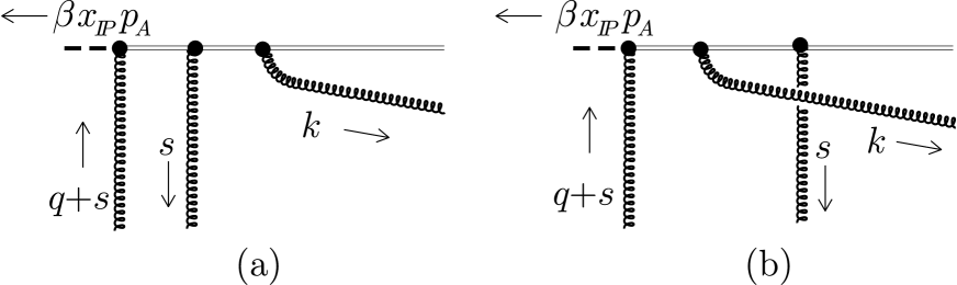
Figure 16: Gluon emission from the eikonal line.

Having seen why certain graphs do not contribute in the $1/x_{\scriptscriptstyle\kern-0.50003ptI\kern-1.25ptP}\to\infty$ limit, we turn to the calculation of the result for a graph that does contribute. Consider the contribution to the gluon Green function $U_{g}$ from the product of the amplitude in Fig. 14(a) with the complex conjugate amplitude of the same form. This contribution can be written as

$$U_{g}^{(0)}(x_{\scriptscriptstyle\kern-0.50003ptI\kern-1.25ptP},\beta,{\mbox{\bf q}},{\mbox{\bf s}},{\mbox{\bf s}}^{\prime}) = {{g_{s}^{4}\,C_{A}^{2}\,(N_{c}^{2}-1)\,p_{A}^{+}}\over{2\,\pi\,\beta\,x_{{\scriptscriptstyle\kern-0.50003ptI\kern-1.25ptP}}}}\int\,{{ds^{+}}\over{2\,\pi}}\,\int\,{{ds^{\prime+}}\over{2\,\pi}}\int\,{{d^{4}k}\over{(2\,\pi)^{4}}}\,2\,\pi\,\delta_{+}(k^{2})\,2\,\pi\,\delta(k^{\prime+})$$ (C.5)

$$\times {{-F^{\mu j}\,M_{\mu\nu}\,F^{\nu j}}\over{\left[s^{+}+i\,\varepsilon\right]\,\left[(k-q-s)^{2}+i\,\varepsilon\right]\,\left[(k-q-s^{\prime})^{2}-i\,\varepsilon\right]\,\left[s^{\prime+}-i\,\varepsilon\right]}}\hskip 2.84544pt,$$

where $F^{\mu j}$ is the gluon operator vertex, $M_{\mu\nu}$ is the polarization tensor associated with the squared amplitude, and the resulting expression for the spin numerator is

$$-F^{\mu j}\,M_{\mu\nu}\,F^{\nu j} = 4\,(k^{-})^{2}\left\{\left(\beta\,x_{\scriptscriptstyle\kern-0.50003ptI\kern-1.25ptP}\,p_{A}^{+}\right)^{2}-{{\beta\,x_{\scriptscriptstyle\kern-0.50003ptI\kern-1.25ptP}\,p_{A}^{+}}\over{k^{-}}}\,\left[({\bf k}-{\bf q}-{\bf s})^{2}+({\bf k}-{\bf q}-{\bf s}^{\prime})^{2}\right]\right.$$ (C.6)

$$\left.+{{\left[({\bf k}-{\bf q}-{\bf s})\cdot({\bf k}-{\bf q}-{\bf s}^{\prime})\right]^{2}}\over{(k^{-})^{2}}}\right\}\hskip 11.38092pt.$$

We may perform the integrations over the plus and minus components of the momentum $k$ by using Eq. (2.14). The $s^{+}$,$s^{\prime+}$ integrations are of the form (C.3). By carrying out this integral we get

$${\cal I}_{+}^{(a)}={1\over{\beta\,{\bf k}^{2}/(1-\beta)+({\bf k}-{\bf q}-{\bf s})^{2}}}\hskip 11.38092pt.$$ (C.7)

Then we obtain

$$U_{g}^{(0)}(x_{\scriptscriptstyle\kern-0.50003ptI\kern-1.25ptP},\beta,{\mbox{\bf q}},{\mbox{\bf s}},{\mbox{\bf s}}^{\prime})={{g_{s}^{4}\,C_{A}^{2}\,(N_{c}^{2}-1)}\over{4\,\pi\,\beta\,(1-\beta)\,x_{{\scriptscriptstyle\kern-0.50003ptI\kern-1.25ptP}}^{2}}}\,\int\,{{d^{2}{\mbox{\bf k}}}\over{(2\,\pi)^{2}}}\,\left\{2\,(\beta\,{\mbox{\bf k}}^{2})^{2}\,+2\,\beta\,(1-\beta)\,{\mbox{\bf k}}^{2}\,\left[({\bf k}-{\bf q}-{\bf s})^{2}\right.\right.$$

$$\left.\left.+({\bf k}-{\bf q}-{\bf s}^{\prime})^{2}\right]+4\,(1-\beta)^{2}\,\left[({\bf k}-{\bf q}-{\bf s})\cdot({\bf k}-{\bf q}-{\bf s}^{\prime})\right]^{2}\right\}$$

$$/\left\{\left[\beta\,{\mbox{\bf k}}^{2}+(1-\beta)\,({\bf k}-{\bf q}-{\bf s})^{2}\right]\,\left[\beta\,{\mbox{\bf k}}^{2}+(1-\beta)\,({\bf k}-{\bf q}-{\bf s}^{\prime})^{2}\right]\right\}\hskip 11.38092pt.$$ (C.8)

We recognize in this expression the contribution to $U_{g}$ from the last term in Eq. (3.75). Indeed, the expression (S0.Ex70) can be recast in the form

$$U_{g}^{(0)}(x_{\scriptscriptstyle\kern-0.50003ptI\kern-1.25ptP},\beta,{\mbox{\bf q}},{\mbox{\bf s}},{\mbox{\bf s}}^{\prime})={{g_{s}^{4}\,C_{A}^{2}\,(N_{c}^{2}-1)}\over{4\,\pi\,\beta\,(1-\beta)\,x_{{\scriptscriptstyle\kern-0.50003ptI\kern-1.25ptP}}^{2}}}\,\int\,{{d^{2}{\mbox{\bf k}}}\over{(2\,\pi)^{2}}}\,{\mbox{Tr}}\left(\psi_{g}^{\dagger}({\mbox{\bf k}},{\mbox{\bf k}}-{\mbox{\bf q}}-{\mbox{\bf s}}^{\prime})\,\psi_{g}({\mbox{\bf k}},{\mbox{\bf k}}-{\mbox{\bf q}}-{\mbox{\bf s}})\right)\hskip 5.69046pt,$$ (C.9)

with $\psi$ being the wave function given in Eq. (3.78).

The other terms in Eq. (3.75) are obtained in a similar way by adding the graphs in which the exchanged gluons attach to the same line and using the color singlet projection (3.47).

Appendix D. An integral representation for the Green functions $U_{a}$

In this appendix we give an integral representation for the Green functions $U_{a}$ alternative to the one given in the text, Eq. (3.74). It is obtained from Eq. (3.74) by performing the trace, introducing a Feynman parameterization to combine the denominators and carrying out the integral over ${\bf k}$. The resulting formulas are lengthy and not as compact as the formulas used in the text. They have the advantages, though, that the spin structure is explicitly worked out and that the cancellation of the singular terms at large ${\bf k}^{2}$ is also explicitly worked out. They may be useful for numerical evaluation.

The functions $U_{a}$ are written as

$$U_{a}(x_{\scriptscriptstyle\kern-0.50003ptI\kern-1.25ptP},\beta,{\mbox{\bf q}},{\mbox{\bf s}},{\mbox{\bf s}}^{\prime}) = {{g_{s}^{4}\,c_{a}(1-\beta)}\over{16\,\pi^{2}\,\beta\,x_{{\scriptscriptstyle\kern-0.50003ptI\kern-1.25ptP}}^{2}}}\,\sum_{i=0}^{3}\,\sum_{j=0}^{3}\,(-1)^{i+j}\,\int_{0}^{1}dx$$ (D.1)

$$\times\,\left({\cal F}_{a,ij}\ln{\cal M}_{a,ij}^{2}+{{{\cal G}_{a,ij}}\over{{\cal M}_{a,ij}^{2}}}\right)\;\;,$$

where the arguments $({\mbox{\bf q}},{\mbox{\bf s}},{\mbox{$\bf s^{{}^{\prime}}$}},\beta,x)$ of the auxiliary functions ${\cal F}$, ${\cal G}$, ${\cal M}$ are suppressed. The color factors $c_{a}$ are given in Eqs. (3.76),(3.77). The summation labels $i,j$ run over the four momentum configurations appearing in the definition of $u_{a}$ (see Eq.(3.75))

$$u_{a}(\beta,{\mbox{\bf k}},{\mbox{\bf q}},{\mbox{\bf s}})=\sum_{i=0}^{3}(-1)^{i}\psi_{a}({\mbox{\bf k}},{\mbox{\bf k}}+{\mbox{${\bf r}^{(i)}_{1}$}})\;\;,$$

where for $i,j=0,1,2,3\;$ ${\bf r}^{(i)}_{1}$,${\bf r}^{(j)}_{2}$ have the values

$${\mbox{${\bf r}^{(i)}_{1}$}}=\{{\mbox{\bf 0}},{\mbox{\bf s}},-{\mbox{\bf q}},-{\mbox{\bf q}}-{\mbox{\bf s}}\}\;,\;\qquad{\mbox{${\bf r}^{(j)}_{2}$}}=\{{\mbox{\bf 0}},{\mbox{$\bf s^{{}^{\prime}}$}},-{\mbox{\bf q}},-{\mbox{\bf q}}-{\mbox{$\bf s^{{}^{\prime}}$}}\}\;\;\;.$$

The expressions for ${\cal F}_{a,ij},$ ${\cal G}_{a,ij}$ and ${\cal M}^{2}_{ij}$ are

$${\cal F}_{a,ij} = f_{a,1}(x,\gamma){\mbox{${\bf r}^{(i)}_{1}$}}\cdot{\mbox{${\bf r}^{(i)}_{1}$}}+f_{a,2}(x,\gamma){\mbox{${\bf r}^{(i)}_{1}$}}\cdot{\mbox{${\bf r}^{(j)}_{2}$}}+\left(x\to(1-x),{\mbox{${\bf r}^{(i)}_{1}$}}\to{\mbox{${\bf r}^{(j)}_{2}$}}\right)$$

$${\cal G}_{a,ij} = g_{a,1}(x,\gamma)({\mbox{${\bf r}^{(i)}_{1}$}}\cdot{\mbox{${\bf r}^{(i)}_{1}$}})^{2}+g_{a,2}(x,\gamma)({\mbox{${\bf r}^{(i)}_{1}$}}\cdot{\mbox{${\bf r}^{(i)}_{1}$}})({\mbox{${\bf r}^{(j)}_{2}$}}\cdot{\mbox{${\bf r}^{(j)}_{2}$}})+g_{a,3}(x,\gamma)({\mbox{${\bf r}^{(i)}_{1}$}}\cdot{\mbox{${\bf r}^{(j)}_{2}$}})^{2}$$

$$+g_{a,4}(x,\gamma)({\mbox{${\bf r}^{(i)}_{1}$}}\cdot{\mbox{${\bf r}^{(j)}_{2}$}})({\mbox{${\bf r}^{(i)}_{1}$}}\cdot{\mbox{${\bf r}^{(i)}_{1}$}})+\left(x\to(1-x),{\mbox{${\bf r}^{(i)}_{1}$}}\to{\mbox{${\bf r}^{(j)}_{2}$}}\right)$$

$${\cal M}^{2}_{ij} = \gamma x(1-\gamma x){\mbox{${\bf r}^{(i)}_{1}$}}\cdot{\mbox{${\bf r}^{(i)}_{1}$}}-\,\gamma^{2}x(1-x){\mbox{${\bf r}^{(i)}_{1}$}}\cdot{\mbox{${\bf r}^{(j)}_{2}$}}+\left(x\to(1-x),{\mbox{${\bf r}^{(i)}_{1}$}}\to{\mbox{${\bf r}^{(j)}_{2}$}}\right)\hskip 5.69046pt,$$

where $\gamma=1-\beta$. The new auxiliary functions $f$ and $g$ are simple polynomials in $x$:

$$f_{q,1} = 4(1-\gamma)x(2-3\gamma x)$$

$$f_{q,2} = ((1-\gamma)(-1+2\gamma-12\gamma^{2}(1-x)x))/\gamma$$

$$g_{q,1} = -2(1-\gamma)\gamma^{2}x^{3}(1-\gamma x)$$

$$g_{q,2} = -(1-\gamma)\gamma^{2}(1-x)x[1-2\gamma(1-x)x]$$

$$g_{q,2} = 2(1-\gamma)\gamma(1-x)x(1-\gamma+2\gamma^{2}(1-x)x)$$

$$g_{q,4} = 2(1-\gamma)\gamma x^{2}(1-\gamma(3-2x)+4\gamma^{2}(1-x)x)$$

in the case of quarks and

$$f_{g,1} = (-2(1-2(1+2\gamma+3\gamma^{2})x+6(\gamma+\gamma^{3})x^{2}))/\gamma$$

$$f_{g,2} = 2(-1+2\gamma-6(1+\gamma^{2})x(1-x))$$

$$g_{g,1} = 2\gamma x^{2}(1+\gamma(-1+x)^{2}-2\gamma^{2}x+\gamma^{3}x^{2})$$

$$g_{g,2} = \gamma\Bigl{(}\Big{[}1-2(1+\gamma^{2})x(1-x)+2\gamma^{3}(1-x)^{2}x^{2}+$$

$$\gamma\big{\{}-1+2x(1-x)(2+x(1-x)\big{\}}\Big{]}\Bigr{)}$$

$$g_{g,3} = 2\Bigl{(}1-2\gamma-2\gamma^{3}(1-x)x+2\gamma^{4}(1-x)^{2}x^{2}+$$

$$\gamma^{2}\big{[}1+2x(1-x)\bigl{\{}1+x(1-x)\bigr{\}}\big{]}\Bigr{)}$$

$$g_{g,4} = -4\gamma x\Bigl{[}1+x+\gamma^{2}(3-2x)x-$$

$$2\gamma^{3}(1-x)x^{2}-\gamma(1+4x^{2}-2x^{3})\Bigr{]}$$

in the case of gluons. The $x$ integral can easily be carried out but the result is simple only for the limiting values ${\mbox{\bf q}}=0,\beta\to 0$ or $\beta\to 1$. The expressions for these cases are given in Sec. 4.2.

References

References

• [1] G. Ingelman and P. Schlein, Phys. Lett.  152B, 256 (1985).
• [2] UA8 Collaboration (A. Brandt et al.), Phys. Lett. B 297, 417 (1992).
• [3] CDF Collaboration (F. Abe et al.), Phys. Rev. Lett. 74, 855 (1995); 78, 2698 (1997); 79, 2636 (1997); D0 Collaboration (S. Abachi et al.), Phys. Rev. Lett. 72, 2332 (1994); 76, 734 (1996).
• [4] ZEUS Collaboration (M. Derrick et al.), Phys. Lett.  B 315, 481 (1993); 332, 228 (1994); 338, 483 (1994); 356, 129 (1995); Z. Phys. C 68, 569 (1995); 70, 391 (1996); H1 Collaboration (T. Ahmed et al.), Nucl. Phys.  B429, 477 (1994); Phys. Lett.  B 348, 681 (1995).
• [5] H1 Collaboration, (C. Adloff et al.), Z. Phys. C 76, 613 (1997); ZEUS Collaboration (J. Breitweg et al.), Eur. Phys. J. C1, 81 (1998).
• [6] ZEUS Collaboration (J. Breitweg et al.), Eur. Phys. J. C6, 43 (1999).
• [7] See, for instance, the review in J.C. Collins, D.E. Soper and G. Sterman, in Perturbative Quantum Chromodynamics, edited by A.H. Mueller (World Scientific, Singapore, 1989).
• [8] J.C. Collins, L. Frankfurt and M. Strikman, Phys. Lett. B 307, 161 (1993); A. Berera and D.E. Soper, Phys. Rev. D 50, 4328 (1994).
• [9] J.C. Collins, Phys. Rev. D 57, 3051 (1998).
• [10] A. Berera and D.E. Soper, Phys. Rev. D 53, 6162 (1996).
• [11] L. Trentadue and G. Veneziano, Phys. Lett. B 323, 201 (1994).
• [12] F. Hautmann, Z. Kunszt and D.E. Soper, Phys. Rev. Lett. 81, 3333 (1998).
• [13] J.D. Bjorken, AIP Conference Proceedings No. 6, Particles and Fields subseries No. 2, edited by M. Bander, G. Shaw and D. Wong (AIP, New York, 1972); J.D. Bjorken and J. Kogut, Phys. Rev.  D 8, 1341 (1973); J.D. Bjorken, preprint SLAC-PUB-7096 (1996), hep-ph/9601363.
• [14] J.C. Collins and D.E. Soper, Nucl.  Phys. B194, 445 (1982).
• [15] G. Curci, W. Furmanski and R. Petronzio, Nucl.  Phys. B175, 27 (1980).
• [16] J. Kogut and D.E. Soper, Phys. Rev.  D 1, 2901 (1970).
• [17] N.N. Nikolaev and B.G. Zakharov, Z. Phys. C 49, 607 (1991); 53, 331 (1992); A.H. Mueller, Nucl.  Phys. B335, 115 (1990); L. Frankfurt and M. Strikman, Phys. Rep. 160, 235 (1988).
• [18] W. Buchmüller and A. Hebecker, Nucl.  Phys. B476, 203 (1996); A. Hebecker, Nucl.  Phys. B505, 349 (1997); W. Buchmüller, T. Gehrmann and A. Hebecker, Nucl.  Phys. B537, 477 (1999).
• [19] M. Wüsthoff, Phys. Rev. D 56 , 4311 (1997); J. Bartels, J. Ellis, H. Kowalski and M. Wüsthoff, Eur. Phys. J. C7, 443 (1999).
• [20] J.D. Bjorken, J. Kogut and D.E. Soper, Phys. Rev.  D 3, 1382 (1971).
• [21] T. Gehrmann and W.J. Stirling, Z. Phys. C 70, 89 (1996); K. Golec-Biernat and J. Kwiecinski, Phys. Lett. B 353, 329 (1995); Z. Kunszt and W.J. Stirling, in Proceedings of the International Workshop on Deep Inelastic Scattering DIS96, Rome, Italy, 1996, edited by G. D’Agostini and A. Nigro (World Scientific, Singapore, 1997), p.240; L. Alvero, J.C. Collins, J. Terron and J. Whitmore, Phys. Rev. D 59, 074022 (1999).
• [22] See, for instance, M.J. Teper, hep-th/9812187; S. Dalley and B. van de Sande, Phys. Rev. Lett. 82, 1088 (1999); C.J. Morningstar and M. Peardon, hep-lat/9901004.
• [23] A.H. Mueller, in Proceedings of the International Workshop on Deep Inelastic Scattering DIS98, Brussels, Belgium, 1998, edited by G. Coremans and R. Roosen (World Scientific, Singapore, 1998), p.3.
• [24] H.L. Lai et al., Phys. Rev. D 55, 1280 (1997).
• [25] J. Ellis and G.G. Ross, Phys. Lett. B 384, 293 (1996); J. Ellis, G.G. Ross and J. Williams, hep-ph/9812385.
• [26] E. Gotsman, E. Levin and U. Maor, Nucl.  Phys. B493, 354 (1997); J. Jalilian-Marian, A. Kovner, A. Leonidov and H. Weigert, Phys. Rev. D 59, 034007 (1999); K. Golec-Biernat and M. Wüsthoff, hep-ph/9903358.