Approximate Analytic Solutions
of RG Equations for Yukawa
and Soft Couplings in SUSY Models

Abstract

We present simple analytical formulae which describe solutions of the RG equations for Yukawa couplings in SUSY gauge theories with the accuracy of a few per cent. Performing the Grassmannian expansion in these solutions, one finds those for all the soft couplings and masses. The solutions clearly exhibit the fixed point behaviour which can be calculated analytically. A comparison with numerical solutions is made.

1 Introduction

The renormalization group equations (RGEs) for the rigid couplings and soft parameters in SUSY gauge theories play a crucial role in applications. Actually, all predictions of the MSSM are based on solutions to these equations in leading and next-to-leading orders [1]. Typically, one has three gauge couplings, one or three Yukawa couplings (for the case of low or high $\tan\beta$, respectively) and a set of soft couplings. In leading order, solutions to the RGE for the gauge couplings are simple; however, already for Yukawa couplings, they are known in an analytical form only for the low $\tan\beta$ case, where only the top coupling is left. Moreover, even in this case solutions for the soft terms look rather cumbersome and difficult to explore [2].

In a recent paper [3], it has been shown that solutions to the RGE for the soft couplings follow from those for the rigid ones in a straightforward way. One takes the solution for the rigid coupling (gauge or Yukawa), substitute instead of the initial conditions their modified expressions

$$\alpha_{i} \Rightarrow \tilde{\alpha}_{i}=\alpha_{i}(1+M_{i}\eta+\bar{M}_{i}\bar{\eta}+2M_{i}\bar{M}_{i}\eta\bar{\eta}),$$ (1)

$$Y_{k} \Rightarrow \tilde{Y}_{k}=Y_{k}(1-A_{k}\eta-\bar{A}_{k}\bar{\eta}+A_{k}\bar{A}_{k}\eta\bar{\eta}+\Sigma_{k}\eta\bar{\eta}).$$ (2)

where $\eta=\theta^{2},\bar{\eta}=\bar{\theta}^{2}$, $\theta$ and $\bar{\theta}$ are the Grassmannian parameters, and expand over these parameters. This gives the solution to the RGEs for the soft couplings.

Hereafter the following notation is used:

$$\alpha_{i}\equiv\frac{g_{i}^{2}}{16\pi^{2}},\ \ Y_{k}\equiv\frac{y_{k}^{2}}{16\pi^{2}}\,,\ \ \Sigma_{k}=\sum_{j=1}^{3}m^{2}_{j}\,.$$ (3)

where $g_{i}$ and $y_{k}$ are the gauge and Yukawa couplings, respectively, and $m_{j}^{2}$ are the soft masses associated with each scalar field.

This procedure, however, assumes that one knows solutions to the RGE for the rigid couplings in the analytic form. For instance, in the case of the MSSM in the low $\tan\beta$ regime this allows one to get solutions for the soft couplings and masses simpler than those known in the literature  (see [3]). At the same time, in many cases such solutions are unknown. Actual examples are the MSSM with high $\tan\beta$ and NMSSM. One is bound to solve the RGEs numerically when the number of coupled equations increases dramatically with the soft terms being included.

Below we propose simple analytical formulae which give an approximate solution to the RGE for Yukawa couplings in an arbitrary SUSY theory with the accuracy of a few per cent. Performing the Grassmannian expansion in these approximate solutions one can get those for the soft couplings in a straightforward way. As an illustration we consider the MSSM in the high $\tan\beta$ regime.

One can immediately see that approximate solutions obtained in this way possess infrared quasi-fixed points [7] which can be found analytically. They appear in the limit when the initial values of the Yukawa couplings are much larger than those for the gauge ones. Then, one can analytically trace how the initial conditions for the soft terms disappear from their solutions in the above  mentioned limit.

The paper is organized as follows. In Sect. 2, we consider the MSSM in the low $\tan\beta$ regime, where all solutions are known analytically and describe briefly the Grassmannian expansion. In Sect. 3, we present our approximate solutions for the Yukawa couplings and obtain those for the soft terms. We also present numerical illustration and compare approximate solutions with the numerical ones. The fixed point behaviour is discussed. Section 4 contains our conclusions. The explicit formulae for the soft couplings and masses are given in Appendices.

2 The MSSM: exact solutions in the low $\tan\beta$ case

Consider the MSSM in the low $\tan\beta$ regime. One has three gauge and one Yukawa coupling. The one-loop RG equations are

$$\dot{\alpha}_{i} = -b_{i}\alpha^{2}_{i},\ \ \ \ b_{i}=(\frac{33}{5},1,-3),\ \ i=1,2,3.$$ (4)

$$\dot{Y}_{t} = Y_{t}\left(\frac{16}{3}\alpha_{3}+3\alpha_{2}+\frac{13}{15}\alpha_{1}-6Y_{t}\right).$$ (5)

with the initial conditions: $\alpha_{i}(0)=\alpha_{0},\ Y_{t}(0)=Y_{0}$, and $t=\ln(M_{X}^{2}/Q^{2})$. Their solutions are given by [2]

$$\alpha_{i}(t)=\frac{\alpha_{0}}{1+b_{i}\alpha_{0}t}\,,\ \ \ Y_{t}(t)=\frac{Y_{0}E(t)}{1+6Y_{0}F(t)}\,,$$ (6)

where

$$E(t) = \prod_{i}(1+b_{i}\alpha_{0}t)^{\displaystyle c_{i}/b_{i}},\ \ \ c_{i}=(\frac{13}{15},3,\frac{16}{3}),$$ (7)

$$F(t) = \int^{t}_{0}E(t^{\prime})dt^{\prime}.$$ (8)

To get solutions for the soft terms, it is enough to perform the substitution $\alpha\to\tilde{\alpha}$ and $Y\to\tilde{Y}$ for the initial conditions in (6) and expand over $\eta$ and $\bar{\eta}$. Expanding the gauge coupling in (6) up to $\eta$ one has (hereafter we assume $M_{i0}=m_{1/2}$)

$$M_{i}(t)=\frac{m_{1/2}}{1+b_{i}\alpha_{0}t}.$$ (9)

Performing the same expansion for the Yukawa coupling and using the relations

$$\left.\frac{d\tilde{E}}{d\eta}\right|_{\eta}=m_{1/2}t\frac{dE}{dt},\ \ \ \left.\frac{d\tilde{F}}{d\eta}\right|_{\eta}=m_{1/2}(tE-F).$$ (10)

one finds the well-known expression [2]

$$A_{t}(t)=\frac{A_{0}}{1+6Y_{0}F}+m_{1/2}\left(\frac{t}{E}\frac{dE}{dt}-\frac{6Y_{0}(tE-F)}{1+6Y_{0}F}\right)\!.$$ (11)

To get the solution for the $\Sigma$ term, one has to make expansion over $\eta$ and $\bar{\eta}$. This can be done with the help of the following relations:

$$\left.\frac{d^{2}\tilde{E}}{d\eta d\bar{\eta}}\right|_{\eta,\bar{\eta}}=m_{1/2}^{2}\frac{d}{dt}\left(t^{2}\frac{dE}{dt}\right),\ \ \ \left.\frac{d^{2}\tilde{F}}{d\eta d\bar{\eta}}\right|_{\eta,\bar{\eta}}=m_{1/2}^{2}t^{2}\frac{dE}{dt}\,.$$ (12)

As a result one has  [3]

$$\Sigma_{t}(t)\!\!\!\!\! = \!\!\!\!\!\frac{\Sigma_{0}\!-A_{0}^{2}}{1\!+6Y_{0}F}+\frac{(A_{0}\!-m_{1/2}6Y_{0}(tE\!-F))^{2}}{(1+6Y_{0}F)^{2}}+m_{1/2}^{2}\left[\frac{d}{dt}\left(\frac{t^{2}}{E}\frac{dE}{dt}\right)\!\!-\!\frac{6Y_{0}}{1\!+6Y_{0}F}t^{2}\frac{dE}{dt}\right]\!.\,$$ (13)

which is much simpler than what one finds in the literature [2], though coinciding with it after some cumbersome algebra.

One can also write down solutions for the individual masses using the Grassmannian expansion of those for the corresponding superfield propagators. For the first two generations one has

$$m^{2}_{Q_{L}} = m_{0}^{2}+\frac{1}{2}m_{1/2}^{2}\left(\frac{16}{3}f_{3}+3f_{2}+\frac{1}{15}f_{1}\right),$$ (14)

$$m^{2}_{U_{R}} = m_{0}^{2}+\frac{1}{2}m_{1/2}^{2}\left(\frac{16}{3}f_{3}+\frac{16}{15}f_{1}\right),$$ (15)

$$m^{2}_{D_{R}} = m_{0}^{2}+\frac{1}{2}m_{1/2}^{2}\left(\frac{16}{3}f_{3}+\frac{4}{15}f_{1}\right),$$ (16)

$$m^{2}_{H_{1}} = m_{0}^{2}+\frac{1}{2}m_{1/2}^{2}\left(3f_{2}+\frac{3}{5}f_{1}\right),$$ (17)

$$m^{2}_{L_{L}} = m_{0}^{2}+\frac{1}{2}m_{1/2}^{2}\left(3f_{2}+\frac{3}{15}f_{1}\right),$$ (18)

$$m^{2}_{E_{R}} = m_{0}^{2}+\frac{1}{2}m_{1/2}^{2}\left(\frac{12}{5}f_{1}\right),$$ (19)

where

$$f_{i}=\frac{1}{b_{i}}\left(1-\frac{1}{(1+b_{i}\alpha_{0}t)^{2}}\right).$$ (20)

The third generation masses get a contribution from the top Yukawa coupling

$$m^{2}_{b_{R}} = m^{2}_{D_{R}},$$ (21)

$$m^{2}_{b_{L}} = m^{2}_{D_{L}}+\Delta/6,$$ (22)

$$m^{2}_{t_{R}} = m^{2}_{U_{R}}+\Delta/3,$$ (23)

$$m^{2}_{t_{L}} = m^{2}_{U_{L}}+\Delta/6,$$ (24)

$$m^{2}_{H_{2}} = m^{2}_{H_{1}}+\Delta/2,$$ (25)

where $\Delta$ is related to $\Sigma_{t}$ (13) by

$$\Delta = \Sigma_{t}-\Sigma_{0}-m_{1/2}^{2}\left[\frac{d}{dt}\left(\frac{t^{2}}{E}\frac{dE}{dt}\right)\right]$$

$$= \frac{\Sigma_{0}-A_{0}^{2}}{1+6Y_{0}F}+\frac{(A_{0}-m_{1/2}6Y_{0}(tE-F))^{2}}{(1+6Y_{0}F)^{2}}-m_{1/2}^{2}\frac{6Y_{0}}{1+6Y_{0}F}t^{2}\frac{dE}{dt}-\Sigma_{0}.$$

With analytic solutions (6,11,13) one can analyze asymptotic and, in particular, find infrared quasi-fixed points [7] which correspond to $Y_{0}\to\infty$

$$Y_{t}^{FP}\!\! = \!\frac{E}{6F},$$ (26)

$$A_{t}^{FP}\!\! = \!m_{1/2}\left(\frac{t}{E}\frac{dE}{dt}-\frac{tE-F}{F}\right),$$ (27)

$$\Sigma_{t}^{FP}\!\! = \!m_{1/2}^{2}\left[\left(\frac{tE-F}{F}\right)^{2}\!\!+\!\frac{d}{dt}\left(\frac{t^{2}}{E}\frac{dE}{dt}\right)\!-\!\frac{t^{2}}{F}\frac{dE}{dt}\right]\!.$$ (28)

One can clearly see that the dependence on $Y_{0},A_{0}$ and $\Sigma_{0}$ disappears from (26)-(28). Some residual dependence on $m_{0}^{2}$ is left for the soft masses and partially cancels with that of $\Delta$.

Below we demonstrate how the same procedure works in the case of approximate solutions. As a realistic example we take the MSSM in the high $\tan\beta$ regime.

3 The MSSM: approximate solutions in high $\tan\beta$ case

The one-loop RGE for the Yukawa couplings in this case look like

$$\dot{Y}_{t} = Y_{t}\left(\frac{16}{3}\alpha_{3}+3\alpha_{2}+\frac{13}{15}\alpha_{1}-6Y_{t}-Y_{b}\right),$$

$$\dot{Y}_{b} = Y_{b}\left(\frac{16}{3}\alpha_{3}+3\alpha_{2}+\frac{7}{15}\alpha_{1}-Y_{t}-6Y_{b}-Y_{\tau}\right),$$

$$\dot{Y}_{\tau} = Y_{\tau}\left(3\alpha_{2}+\frac{9}{5}\alpha_{1}-3Y_{b}-4Y_{\tau}\right).$$

Since the exact solution is absent and might be too cumbersome, we look for an approximate one in a simple form similar to that of (6).

3.1 The choice of approximate solution

In choosing approximate solutions we follow the idea of [8] where an approximate solution for $Y_{t}$ and $Y_{b}$ ignoring $Y_{\tau}$ has been proposed. Our suggestion is to consider separate brackets for each propagator entering into the Yukawa vertex. Then, one has the following expressions for the Yukawa couplings:

$$Y_{t} = \frac{\displaystyle Y_{t0}E_{t}}{\displaystyle[1+A(Y_{t0}F_{t}+Y_{b0}F_{b})]^{1/A}[1+2BY_{t0}F_{t}]^{1/B}[1+3CY_{t0}F_{t}]^{1/C}},\quad\frac{1}{A}\!+\!\frac{1}{B}\!+\!\frac{1}{C}\!=\!1$$

$$Y_{b} = \frac{\displaystyle Y_{b0}E_{b}}{\displaystyle[1+A(Y_{t0}F_{t}+Y_{b0}F_{b})]^{1/A}[1+2BY_{b0}F_{b}]^{1/B}[1+C(3Y_{b0}F_{b}+Y_{\tau 0}F_{\tau})]^{1/C}},$$

$$Y_{\tau} = \frac{\displaystyle Y_{\tau 0}E_{\tau}}{\displaystyle[1+A^{\prime}Y_{\tau 0}F_{\tau}]^{1/A^{\prime}}[1+2B^{\prime}Y_{\tau 0}F_{\tau}]^{1/B^{\prime}}[1+C(3Y_{b0}F_{b}+Y_{\tau 0}F_{\tau})]^{1/C}},\quad\frac{1}{A^{\prime}}\!+\!\frac{1}{B^{\prime}}\!+\!\frac{1}{C}\!=\!1$$

where the brackets correspond to the $Q,U,H_{2}$, $Q,D,H_{1}$ and $L,E,H_{1}$ propagators, respectively. Here $E_{t}$ and $F_{t}$ are given by (7) and (8) and $E_{b}$ and $E_{\tau}$ have the same form but with $c_{i}^{(b)}=(7/15,3,16/3)$ and $c_{i}^{(\tau)}=(9/5,3,0)$, respectively.

The brackets are organized so that they reproduce the contributions of particular diagrams to the corresponding anomalous dimensions. The coefficients $A,B,C,A^{\prime}$ and $B^{\prime}$ are arbitrary and their precise values are not so important. When Yukawa couplings $Y_{i0}$ are small enough, one can make expansion in each bracket, and the dependence of these coefficients disappears. However, for large couplings, which are of interest for us because of the fixed points, we have some residual dependence. The requirement that the sum of exponents equals 1 follows from a comparison with RGEs. Solutions are close to the exact ones when the brackets are roughly equal to each other. Apparently, since $F_{\tau}<F_{t}\sim F_{b}$ and $Y_{\tau}\leq Y_{b}\leq Y_{t}$ one cannot completely satisfy this requirement. Our choice of the coefficients $A,B,C,A^{\prime}$ and $B^{\prime}$ is dictated mainly by simplicity. In the following we choose them as

$$\!\!B=A,C=2/3A\! \rightarrow A=7/2,\ B=7/2,\ C=7/3,$$ (29)

$$\!\!B^{\prime}=A^{\prime}/2\! \rightarrow A^{\prime}=21/4,\ B^{\prime}=21/8.$$ (30)

This gives approximate solutions like

$$Y_{t}\! \approx \!\!\frac{\displaystyle Y_{t0}E_{t}}{\displaystyle\left[1+\!\frac{7}{2}(Y_{t0}F_{t}+Y_{b0}F_{b})\right]^{2/7}\!\!\left[1+7Y_{t0}F_{t}\right]^{5/7}},$$ (31)

$$Y_{b}\! \approx \!\!\frac{\displaystyle Y_{b0}E_{b}}{\displaystyle\left[1+\frac{7}{2}(Y_{t0}F_{t}+Y_{b0}F_{b})\right]^{2/7}\!\!\left[1+7Y_{b0}F_{b}\right]^{2/7}\left[1+\frac{7}{3}(3Y_{b0}F_{b}+Y_{\tau 0}F_{\tau})\right]^{3/7}},$$ (32)

$$Y_{\tau}\! \approx \!\!\frac{\displaystyle Y_{\tau 0}E_{\tau}}{\displaystyle\left[1\!+\!\frac{21}{4}Y_{\tau 0}F_{\tau}\right]^{4/7}\!\!\left[1\!+\!\frac{7}{3}(3Y_{b0}F_{b}\!+\!Y_{\tau 0}F_{\tau})\right]^{3/7}}.\,$$ (33)

Solutions for $A_{i}$ and $\Sigma_{i}$ can be obtained by Grassmannian expansion with the initial conditions

$$A_{i}(0)=A_{0},\ \ \Sigma_{i}(0)=\Sigma_{0}.$$ (34)

These initial conditions correspond to the so-called universality hypothesis which we follow in our numerical illustration for simplicity. However, one can choose arbitrary initial conditions for the soft terms when needed. It leads to an obvious modification of the formulae.

One can get also the corresponding solutions for the individual soft masses. This can be achieved either by Grassmannian expansion of the corresponding brackets in (31)-(33), or by expressing the masses through the $\Sigma$s in an exact way. The second way gives a slightly better agreement with numerical solutions (see below). We present the explicit expressions for the soft terms and masses in Appendix A.

3.2 Numerical analysis

We start by investigating the precision of approximate solutions for the Yukawa couplings. To estimate the accuracy, we introduce a relative error which is defined as

$$\varepsilon=\frac{Y_{approx}-Y_{numeric}}{Y_{numeric}},$$ (35)

and corresponds to the $M_{Z}$ scale ($t=66$) at the end of the integration range. The accuracy for the solutions of soft terms is defined in the same way.

Let us take at the beginning all three Yukawa couplings to be equal at the GUT scale and to have their common value $Y_{0}$ in the range $(.01\div 25)\alpha_{0}$. The upper limit is taken in order not to leave the perturbativity regime. We find that for $Y_{0}\leq\alpha_{0}$ the approximation errors are less than $3\%$ for all $Y$’s. While for $Y_{t}$ it remains smaller than $2\%$ over the whole range of initial values at the GUT scale, for $Y_{b}$ the error increases up to $4\%$ and for $Y_{\tau}$ up to $14\%$ (for large values of $Y_{0}$). It is worth mentioning that for small $Y_{0}$ (around $\alpha_{0}/2$ and below) the accuracy is very good (fractions of per cent or better).

Consider now $Y_{b0}=Y_{\tau 0}=Y_{0}\leq 10\alpha_{0}$ and let the top Yukawa coupling vary within the limits $1\leq Y_{t0}/Y_{0}\leq 10$ in order to examine the applicability of our formulae. In this case the accuracy it is spoilt a little bit with increasing initial values. Namely, the error for $Y_{t}$ increases up to $10\%$, and for $Y_{b}$ and $Y_{\tau}$ up to $20\%$. However, if one keeps $Y_{0}$ in the range $(1/100\div 1/2)\alpha_{0}$ the accuracy for $Y_{t}$ remains better than $3\%$, and for $Y_{b}$ and $Y_{\tau}$ better than $10\%$.

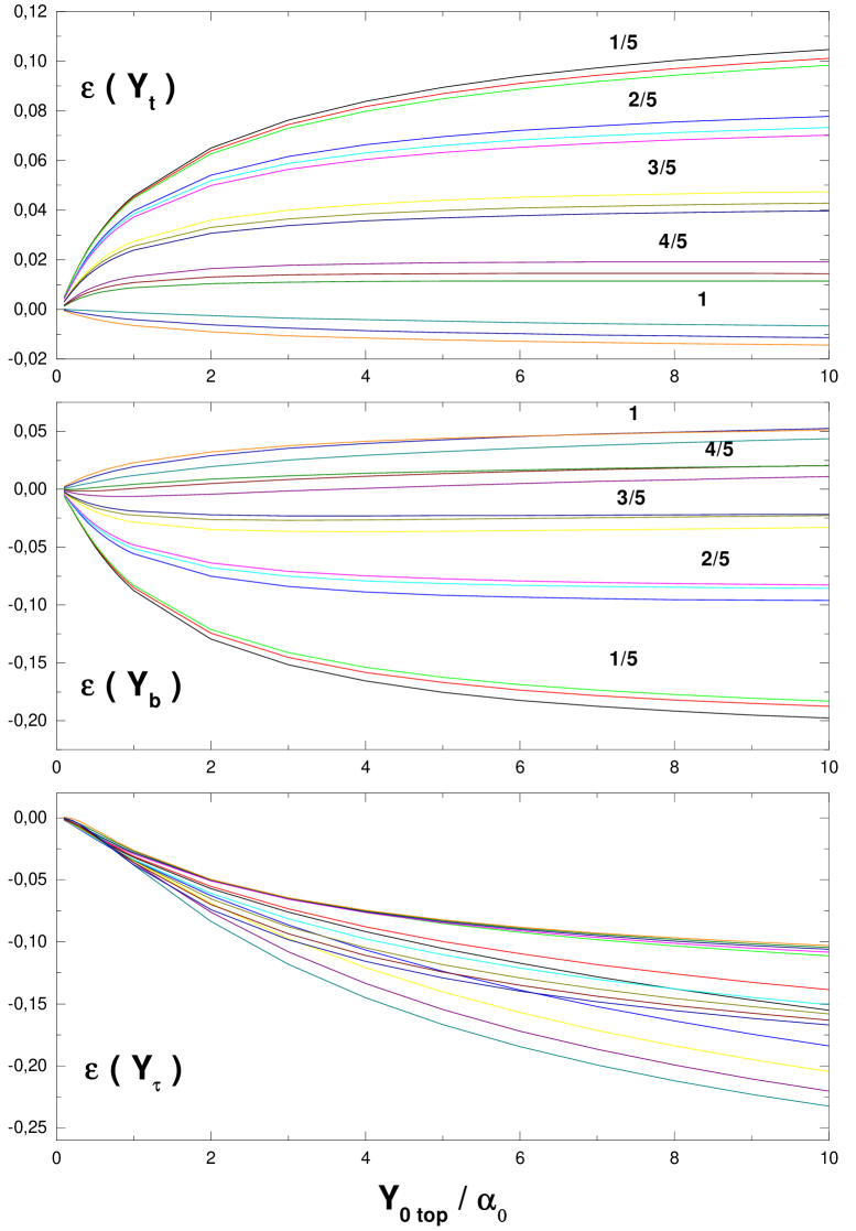
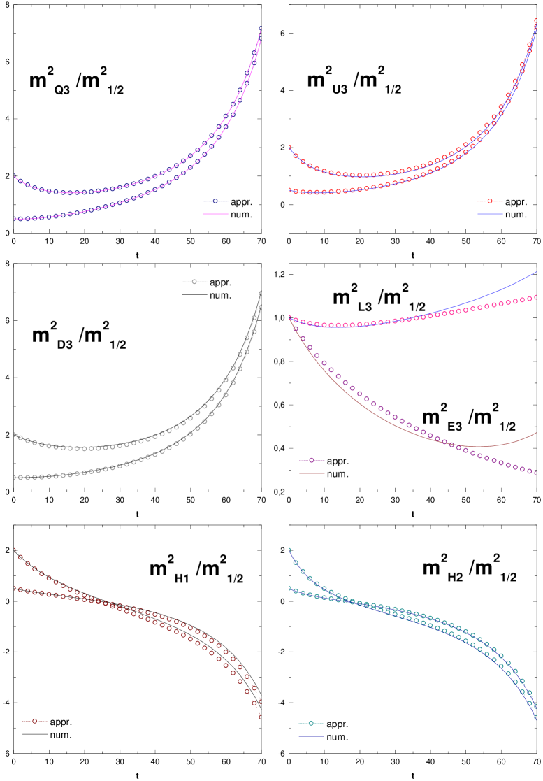
Figure 1: Left side: $Y_{t}$, $Y_{b}$ and $Y_{\tau}$ approximation errors. Numerical labels show the ratio $Y_{b0}/Y_{t0}$ for the corresponding groups of curves (split by different values of $Y_{\tau 0}$). Right side: Comparison of approximate and numerical solutions for the soft masses. The curves correspond to the following choice of initial conditions: $A_{0}=0$, $m^{2}_{0}=(1/2)m^{2}_{1/2}$ and $m^{2}_{0}=2m^{2}_{1/2}$, $Y_{t0}=5\alpha_{0},\,Y_{b0}=Y_{\tau 0}=2\alpha_{0}$. Slepton masses are shown only for $m^{2}_{0}=m^{2}_{1/2}$. Dotted lines correspond to analytical approximation, solid lines to numerical solution.

The particular case considered above seems to have the worst accuracy. This is not surprising since our approximate formulae are supposed to work best of all when all three Yukawa couplings are nearly equal. If we keep $Y_{\tau 0}\leq Y_{b0}\leq Y_{t0}$ and the relative ratios less than $5$, we get an average error of less than $5\%$ for $Y_{t}$, about $5\%$ for $Y_{b}$ and $10\%$ for $Y_{\tau}$. This statement is illustrated in Fig.1. For each Yukawa coupling we have plotted the error as a function of $Y_{t0}$ in the range $(1/10\div 10)\alpha_{0}$. The ratios are kept within the region $1\leq Y_{t0}/Y_{b0}\leq 5$ and $1\leq Y_{b0}/Y_{\tau 0}\leq 3$.

Further on, we narrow the range of initial values up to $(1/10\div 10)\alpha_{0}$ because the errors (defined as in (35)) come to an asymptotic value for $Y_{0}>10\alpha_{0}$ and almost vanish for $Y_{0}<\alpha_{0}/10$. The comparison of numerical and approximated solutions is shown in Fig.2 for three different sets of $Y_{0}$’s. The approximate solutions follow the numerical ones quite well, preserving their shape, and they have a high accuracy, especially in the case of equal Yukawa couplings at the GUT scale. However, as can be seen from the top of Fig. 2, one can take arbitrary initial conditions for the Yukawa couplings, in particular those which are needed to fit the $t/b/\tau$ masses, and to use our approximate solutions for these purposes.

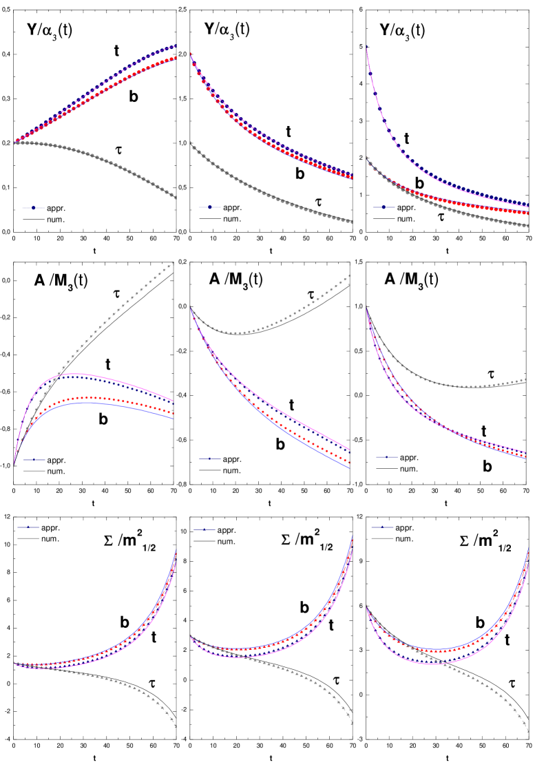
Figure 2: Comparison of approximate and numerical solutions for $Y$, $A$ and $\Sigma$. Evolution of the soft terms $A$ and $\Sigma$ has been plotted for $Y_{t0}=5\alpha_{0}\,,Y_{b0}=Y_{\tau 0}=2\alpha_{0}$. Dotted lines correspond to analytical approximation, solid lines to numerical solution.

For the soft couplings, $A$, we take the initial values at the GUT scale to be $A_{0}=(-2,-1,0,1,2)m_{1/2}$ and leave $Y_{0}$s in the narrow range as above. Then, we get an accuracy of $(3\div 5)\%$ for $A_{t}$ and $A_{b}$. For $A_{\tau}$ the approximation is worse when $A_{0}$ is taken to be negative or smaller than $m_{1/2}$ (see Fig. 2), but things go better for large initial values of $A_{0}$ and we get an accuracy of about $10\%$. Again it should be mentioned that this is an accuracy at the end point where $A_{\tau}$ itself is close to 0 and the accuracy defined as (35) merely gives an odd hint of the precision. Along the curves the accuracy is much better. In Fig.2 we have plotted the behaviour of $A_{t}$, $A_{b}$ and $A_{\tau}$ for three different initial values of $A_{0}$, namely $\{-m_{1/2},0,m_{1/2}\}$ and for one set of $Y_{0}$s. As for the $\Sigma$’s, keeping the range of parameter space for $Y_{0}$ and $A_{0}$ as above, we get an accuracy of typically $2\%$ for $\Sigma_{t}$ (even better for fairly equal $Y_{0}$s). For $\Sigma_{b}$ the precision is around $4\%$. With $\Sigma_{\tau}$ we get into the same troubles as for $A_{\tau}$. The approximation becomes good (about $10\%$) only for a large enough ratio of $m^{2}_{0}/m^{2}_{1/2}$. The approximation errors for $A$’s and $\Sigma$’s are linked with those for $Y$. If one considers only the sets of small initial values for $Y_{0}$ (less than $\alpha_{0}/2$), then $\Sigma$’s are approximated with a precision better than $1\%$, regardless of the $A_{0}$ values. The precision for $\Sigma$ increases with $A_{0}$, but this dependence is not so striking as the one on $Y_{0}$.

The approximate formulae for the soft masses may be derived from $\Sigma$ using (39)-(45). In this case the approximate solutions give an accuracy of about $1\div 3\%$ for $m^{2}_{Q_{3}}$, $m^{2}_{U_{3}}$ and $(3\div 5)\%$ for $m^{2}_{D_{3}}$. For the Higgs masses we get a good approximation (of about $5\%$ on average) for $m^{2}_{H_{2}}$, and a satisfactory one for $m^{2}_{H_{1}}$ (typically $10\%$). This accuracy is almost insensitive to the $A_{0}$ variation (we took it to be in the range $(-2\div 2)m_{1/2}$) and on the ratio $m^{2}_{0}/m^{2}_{1/2}$ (taken to be $0.5\div 2$). The slepton masses (see Fig. 1) are not approximated properly in an analogous way. This is mainly due to the less accurate approximation of $Y_{\tau}$.

As a concluding remark on numerical analysis, it should be mentioned that one has a rather good approximation for small (less than $\alpha_{0}/2$) initial values of the Yukawa couplings. For larger values of $Y$’s one has a good approximation especially in the case of unification of the Yukawa couplings.

3.3 The fixed points

One can easily see that solutions (31)-(33) exhibit the quasi-fixed point behaviour when the initial values $Y_{t0}=Y_{b0}=Y_{\tau 0}\geq\alpha_{0}$. In this case, one can drop 1 in the denominator and the resulting expressions become independent of the initial conditions

$$Y_{t}^{FP} \approx \frac{E_{t}}{\displaystyle\left[\frac{7}{2}(F_{t}+F_{b})\right]^{2/7}\!\!\left[7F_{t}\right]^{5/7}},$$ (36)

$$Y_{b}^{FP} \approx \frac{\displaystyle E_{b}}{\displaystyle\left[\frac{7}{2}(F_{t}+F_{b})\right]^{2/7}\!\!\left[7F_{b}\right]^{2/7}\!\!\left[\frac{7}{3}(3F_{b}+F_{\tau})\right]^{3/7}},$$ (37)

$$Y_{\tau}^{FP} \approx \frac{\displaystyle E_{\tau}}{\displaystyle\left[\frac{21}{4}F_{\tau}\right]^{4/7}\!\!\left[\frac{7}{3}(3F_{b}+F_{\tau})\right]^{3/7}}.$$ (38)

These expressions being expanded over the Grassmannian variables give the quasi-fixed points for the soft terms and masses. The explicit expressions are presented in Appendix B.

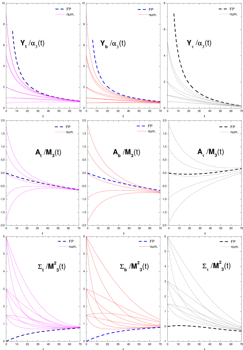
Figure 3: The IRQFP behaviour for Yukawa couplings, soft terms $A_{t,b,\tau}$,and $\Sigma$’s. Numerical solutions for all $A$’s are done for $Y_{t0}=5\alpha_{0}$, $Y_{b0}=Y_{\tau 0}=2\alpha_{0}$. For $\Sigma$ we took $A_{0}=0$, three different sets of $Y_{0}$’s and $m^{2}_{0}$. Dotted lines are the IRQFP from eqs.(36-38) and Appendix B.

We see that the IRQFP behaviour is sharply expressed for $Y_{t}$ and $Y_{b}$ (see Fig. 3), and our approximate solution describes the fixed point line well. The same takes place for the corresponding $A$s and $\Sigma$s. For $Y_{\tau},A_{\tau}$ and $\Sigma_{\tau}$ the accuracy is worse, however, the solution is still reliable. The soft mass terms there exhibit the same IRQFP behaviour, though some residual dependence on the initial conditions is left in full analogy with the exact solutions in the low $\tan\beta$ case. The approximate solutions allow one to calculate the IRQFP analytically.

One can see that the fixed points for the soft terms naturally follow from the Grassmannian expansion of our approximate solutions (36)-(38) and they inherit their stability properties, as has been shown in [9]. In particular, the behaviour of $\Sigma$s essentially repeats that of the Yukawa couplings in agreement with [10].

The existence of the IRQFPs allows one to make predictions for the soft masses without exact knowledge of the initial conditions. This property has been widely used (see, for example, [11]) and though the IRQFPs give a slightly larger top mass when imposing $b-\tau$ unification, it is still possible to fit the quark masses within the error-bars and to make predictions for the Higgs and sparticle spectrum [12]. This explains general interest in the IRQFPs.

4 Discussion

We hope to convince the reader that the approximate solutions presented above reproduce the behaviour of the Yukawa couplings with good precision in the whole integration region and for a large range of initial values. Relative accuracy is typically a few per cent and is worse only at the end of the integration region mainly due to the smallness of the quantities themselves. Moreover, we have shown how the approximate solutions for the soft terms and masses follow from those for the rigid couplings. This demonstrates how the Grassmannian expansion, advocated in [3], works in the case of approximate solutions as well.

For illustration we have considered universal initial conditions for the soft terms. In recent time there appeared some interest in non-universal boundary conditions. Non-universality can also be included in our formulae at the expense of changing (10) and (34) using the same substitution rules, see (1) and (2).

Since the form of our approximate solutions has been ”guessed” ad hoc starting from some reasonable arguments, there is no direct way to improve them. However, one can imagine more constructive derivation of those solutions which would allow one to make corrections. Needless to say that it is enough to construct a solution for the rigid terms. Solutions for the soft terms will follow automatically.

Acknowledgement

We would like to thank A.V.Gladyshev for valuable discussions. Financial support from RFBR grants # 99-02-16650 and # 96-15-96030 is kindly acknowledged.

Appendix A

We here present approximate expressions for the soft couplings and masses corresponding to (31)-(33):

$$M_{i} = \frac{m_{1/2}}{1+b_{i}\alpha_{0}t},$$

$$A_{t} \approx A_{0}\left(1-\frac{Y_{t0}F_{t}+Y_{b0}F_{b}}{1+\frac{7}{2}(Y_{t0}F_{t}+Y_{b0}F_{b})}-\frac{5Y_{t0}F_{t}}{1+7Y_{t0}F_{t}}\right)$$

$$- m_{1/2}\left(\frac{t}{E_{t}}\frac{dE_{t}}{dt}-\frac{Y_{t0}(tE_{t}-F_{t})+Y_{b0}(tE_{b}-F_{b})}{1+\frac{7}{2}(Y_{t0}F_{t}+Y_{b0}F_{b})}-\frac{5Y_{t0}(tE_{t}-F_{t})}{1+7Y_{t0}F_{t}}\right)$$

$$A_{b} \approx A_{0}\left(1-\frac{Y_{t0}F_{t}+Y_{b0}F_{b}}{1+\frac{7}{2}(Y_{t0}F_{t}+Y_{b0}F_{b})}-\frac{2Y_{b0}F_{b}}{1+7Y_{b0}F_{b}}-\frac{3Y_{b0}F_{b}+Y_{\tau 0}F_{\tau}}{1+\frac{7}{3}(3Y_{b0}F_{b}+Y_{\tau 0}F_{\tau})}\right)$$

$$- m_{1/2}\left(\frac{t}{E_{b}}\frac{dE_{b}}{dt}-\frac{Y_{t0}(tE_{t}-F_{t})+Y_{b0}(tE_{b}-F_{b})}{1+\frac{7}{2}(Y_{t0}F_{t}+Y_{b0}F_{b})}\right.$$

$$- \!\left.\frac{2Y_{b0}(tE_{b}-\!F_{b})}{1+7Y_{b0}F_{b}}-\!\frac{3Y_{b0}(tE_{b}-\!F_{b})+Y_{\tau 0}(tE_{\tau}-\!F_{\tau})}{1+\frac{7}{3}(3Y_{b0}F_{b}+Y_{\tau 0}F_{\tau})}\right)$$

$$A_{\tau} \approx A_{0}\left(1-\frac{3Y_{\tau 0}F_{\tau}}{1+\frac{21}{4}Y_{\tau 0}F_{\tau}}-\frac{3Y_{b0}F_{b}+Y_{\tau 0}F_{\tau}}{1+\frac{7}{3}(3Y_{b0}F_{b}+Y_{\tau 0}F_{\tau})}\right)$$

$$- m_{1/2}\left(\frac{t}{E_{\tau}}\frac{dE_{\tau}}{dt}-\frac{3Y_{\tau 0}(tE_{\tau}-F_{\tau})}{1+\frac{21}{4}Y_{\tau 0}F_{\tau}}-\frac{3Y_{b0}(tE_{b}-F_{b})+Y_{\tau 0}(tE_{\tau}-F_{\tau})}{1+\frac{7}{3}(3Y_{b0}F_{b}+Y_{\tau 0}F_{\tau})}\right)$$

$$\Sigma_{t} \approx \Sigma_{0}\left(1-\frac{Y_{t0}F_{t}+Y_{b0}F_{b}}{1+\frac{7}{2}(Y_{t0}F_{t}+Y_{b0}F_{b})}-\frac{5Y_{t0}F_{t}}{1+7Y_{t0}F_{t}}\right)$$

$$-\frac{A_{0}^{2}Y_{t0}F_{t}\!-\!2A_{0}Y_{t0}m_{1/2}(tE_{t}\!-\!F_{t})\!+\!Y_{t0}m_{1/2}^{2}t^{2}\frac{dE_{t}}{dt}\!+\!A_{0}^{2}Y_{b0}F_{b}\!-\!2A_{0}Y_{b0}m_{1/2}(tE_{b}\!-\!F_{b})\!+\!Y_{b0}m_{1/2}^{2}t^{2}\frac{dE_{b}}{dt}}{1\!+\!\frac{7}{2}(Y_{t0}F_{t}\!+\!Y_{b0}F_{b})}$$

$$- \frac{5}{1+7Y_{t0}F_{t}}\left(A_{0}^{2}Y_{t0}F_{t}-2A_{0}Y_{t0}m_{1/2}(tE_{t}-F_{t})+Y_{t0}m_{1/2}^{2}t^{2}\frac{dE_{t}}{dt}\right)$$

$$+ \!\!\frac{\frac{7}{2}}{\bigl{(}1\!+\!\frac{7}{2}(Y_{t0}F_{t}\!+\!Y_{b0}F_{b})\bigr{)}^{2}}\!\Bigl{(}-A_{0}Y_{t0}F_{t}\!+\!Y_{t0}m_{1/2}(tE_{t}\!-\!F_{t})\Bigr{.}\Bigl{.}-A_{0}Y_{b0}F_{b}+\!Y_{b0}m_{1/2}(tE_{b}-F_{b})\Bigr{)}^{2}\!\!$$

$$\!+\!m_{1/2}^{2}\frac{d}{dt}\!\left(\frac{t^{2}}{E_{t}}\frac{dE_{t}}{dt}\right)+\frac{35}{\bigl{(}1+7Y_{t0}F_{t}\bigr{)}^{2}}\Bigl{(}-A_{0}Y_{t0}F_{t}+Y_{t0}m_{1/2}(tE_{t}-F_{t})\Bigr{)}^{2}$$

$$\Sigma_{b} \approx \Sigma_{0}\left(1-\frac{Y_{t0}F_{t}+Y_{b0}F_{b}}{1+\frac{7}{2}(Y_{t0}F_{t}+Y_{b0}F_{b})}-\frac{2Y_{b0}F_{b}}{1+7Y_{b0}F_{b}}\ -\frac{3Y_{b0}F_{b}+Y_{\tau 0}F_{\tau}}{1+\frac{7}{3}(3Y_{b0}F_{b}+Y_{\tau 0}F_{\tau})}\right)$$

$$- \!\frac{1}{1\!+\!\frac{7}{2}(Y_{t0}F_{t}+\!Y_{b0}F_{b})}\Bigl{(}A_{0}^{2}Y_{t0}F_{t}-\!2A_{0}Y_{t0}m_{1/2}(tE_{t}\!-\!F_{t})\Bigr{.}$$

$$\Bigl{.}+Y_{t0}m_{1/2}^{2}t^{2}\frac{dE_{t}}{dt}+\!A_{0}^{2}Y_{b0}F_{b}-2A_{0}Y_{b0}m_{1/2}(tE_{b}-F_{b})+Y_{b0}m_{1/2}^{2}t^{2}\frac{dE_{b}}{dt}\Bigr{)}$$

$$-\frac{2}{1+7Y_{b0}F_{b}}\left(A_{0}^{2}Y_{b0}F_{b}-2A_{0}Y_{b0}m_{1/2}(tE_{b}-F_{b})+Y_{b0}m_{1/2}^{2}t^{2}\frac{dE_{b}}{dt}\right)$$

$$- \frac{1}{1+\frac{7}{3}(3Y_{b0}F_{b}+Y_{\tau 0}F_{\tau})}\Bigl{(}3A_{0}^{2}Y_{b0}F_{b}+A_{0}^{2}Y_{\tau 0}F_{\tau}-6A_{0}Y_{b0}m_{1/2}(tE_{b}-F_{b})\Bigr{.}$$

$$\Bigl{.}-2A_{0}Y_{\tau 0}m_{1/2}(tE_{\tau}-F_{\tau})+3Y_{b0}m_{1/2}^{2}t^{2}\frac{dE_{b}}{dt}+Y_{\tau 0}m_{1/2}^{2}t^{2}\frac{dE_{\tau}}{dt}\Bigr{)}$$

$$+ \!\!\frac{{\frac{7}{2}}\!\Bigl{(}-A_{0}Y_{t0}F_{t}\!+\!Y_{t0}m_{1/2}(tE_{t}\!-\!F_{t})-A_{0}Y_{b0}F_{b}+\!Y_{b0}m_{1/2}(tE_{b}-F_{b})\Bigr{)}^{2}}{\bigl{(}1\!+\!\frac{7}{2}(Y_{t0}F_{t}\!+\!Y_{b0}F_{b})\bigr{)}^{2}}$$

$$\!\!+\!m_{1/2}^{2}\frac{d}{dt}\!\left(\frac{t^{2}}{E_{b}}\frac{dE_{b}}{dt}\right)+14\frac{\bigl{(}-A_{0}Y_{b0}F_{b}+Y_{b0}m_{1/2}(tE_{b}-F_{b})\bigr{)}^{2}}{\bigl{(}1+7Y_{b0}F_{b}\bigr{)}^{2}}$$

$$+ \!\frac{{\frac{7}{3}}\Bigl{(}-3A_{0}Y_{b0}F_{b}-\!A_{0}Y_{\tau 0}F_{\tau}+3Y_{b0}m_{1/2}(tE_{b}-F_{b})+Y_{\tau 0}m_{1/2}(tE_{\tau}-F_{\tau})\Bigr{)}^{2}}{\bigl{(}1\!+\!\frac{7}{3}(3Y_{b0}F_{b}\!+\!Y_{\tau 0}F_{\tau})\bigr{)}^{2}}$$

$$\Sigma_{\tau} \approx \Sigma_{0}\left(1-\frac{3Y_{\tau 0}F_{\tau}}{1+\frac{21}{4}Y_{\tau 0}F_{\tau}}-\frac{3Y_{b0}F_{b}+Y_{\tau 0}F_{\tau}}{1+\frac{7}{3}(3Y_{b0}F_{b}+Y_{\tau 0}F_{\tau})}\right)$$

$$- \frac{3}{1+\frac{21}{4}Y_{\tau 0}F_{\tau}}\Bigl{(}A_{0}^{2}Y_{\tau 0}F_{\tau}-2A_{0}Y_{\tau 0}m_{1/2}(tE_{\tau}-F_{\tau})+Y_{\tau 0}m_{1/2}^{2}t^{2}\frac{dE_{\tau}}{dt}\Bigr{)}$$

$$- \!\!\frac{1}{1+\frac{7}{3}(3Y_{b0}F_{b}+Y_{\tau 0}F_{\tau})}\Bigl{(}3A_{0}^{2}Y_{b0}F_{b}\!+\!A_{0}^{2}Y_{\tau 0}F_{\tau}\!-\!6A_{0}Y_{b0}m_{1/2}(tE_{b}\!-\!F_{b})\!+\!3Y_{b0}m_{1/2}^{2}t^{2}\frac{dE_{b}}{dt}\Bigr{.}$$

$$\Bigl{.}-2A_{0}Y_{\tau 0}m_{1/2}(tE_{\tau}-F_{\tau})+Y_{\tau 0}m_{1/2}^{2}t^{2}\frac{dE_{\tau}}{dt}\Bigr{)}+\frac{63}{4}\frac{\bigl{(}-A_{0}Y_{\tau 0}F_{\tau}+Y_{\tau 0}m_{1/2}(tE_{\tau}-F_{\tau})\bigr{)}^{2}}{\bigl{(}1+\frac{21}{4}Y_{\tau 0}F_{\tau}\bigr{)}^{2}}$$

$$+ \frac{\frac{7}{3}\bigl{(}-\!3A_{0}Y_{b0}F_{b}-\!A_{0}Y_{\tau 0}F_{\tau}+3Y_{b0}m_{1/2}(tE_{b}-F_{b})+Y_{\tau 0}m_{1/2}(tE_{\tau}-F_{\tau})\bigr{)}^{2}}{\bigl{(}1+\frac{7}{3}(3Y_{b0}F_{b}+Y_{\tau 0}F_{\tau})\bigr{)}^{2}}$$

$$\qquad\qquad+m_{1/2}^{2}\frac{d}{dt}\left(\frac{t^{2}}{E_{\tau}}\frac{dE_{\tau}}{dt}\right).$$

To find the individual soft masses one can formally perform integration of the RG equations and express the masses through $\Sigma$s solving a system of linear algebraic equations. This gives

$$m_{Q_{3}}^{2}\!\! = \!\!\frac{13}{61}m^{2}_{0}+m_{1/2}^{2}\left(\frac{64}{61}f_{3}+\frac{87}{122}f_{2}-\frac{11}{122}f_{1}\right)\!\!+\frac{1}{122}\left(17\Sigma_{t}+20\Sigma_{b}-5\Sigma_{\tau}\right)$$ (39)

$$m_{U_{3}}^{2}\!\! = \!\!\frac{7}{61}m^{2}_{0}+m_{1/2}^{2}\left(\frac{72}{61}f_{3}-\frac{54}{61}f_{2}+\frac{72}{305}f_{1}\right)\!\!+\frac{1}{122}\left(42\Sigma_{t}-8\Sigma_{b}+2\Sigma_{\tau}\right)$$ (40)

$$m_{D_{3}}^{2}\!\! = \!\!\frac{19}{61}m^{2}_{0}+m_{1/2}^{2}\left(\frac{56}{61}f_{3}-\frac{42}{61}f_{2}+\frac{56}{305}f_{1}\right)\!\!+\frac{1}{122}\left(-8\Sigma_{t}+48\Sigma_{b}-12\Sigma_{\tau}\right)$$ (41)

$$m_{H_{1}}^{2}\!\! =\!\! -\frac{32}{61}m^{2}_{0}+m_{1/2}^{2}\left(-\frac{120}{61}f_{3}\!-\frac{3}{122}f_{2}\!-\frac{57}{610}f_{1}\right)\!\!+\frac{1}{122}\left(-9\Sigma_{t}\!+54\Sigma_{b}\!+17\Sigma_{\tau}\right)$$ (42)

$$m_{H_{2}}^{2}\!\! = \!\!-\frac{20}{61}m^{2}_{0}+m_{1/2}^{2}\left(-\frac{136}{61}f_{3}+\frac{21}{122}f_{2}-\frac{89}{610}f_{1}\right)\!\!+\frac{1}{122}\left(63\Sigma_{t}-12\Sigma_{b}+3\Sigma_{\tau}\right)$$ (43)

$$m_{L_{3}}^{2}\!\! = \!\!\frac{31}{61}m^{2}_{0}+m_{1/2}^{2}\left(\frac{40}{61}f_{3}+\frac{123}{122}f_{2}-\frac{103}{610}f_{1}\right)\!\!+\frac{1}{122}\left(3\Sigma_{t}-18\Sigma_{b}+35\Sigma_{\tau}\right)$$ (44)

$$m_{E_{3}}^{2}\!\! = \!\!\frac{1}{61}m^{2}_{0}+m_{1/2}^{2}\left(\frac{80}{61}f_{3}-\frac{60}{61}f_{2}+\frac{16}{61}f_{1}\right)\!\!+\frac{1}{122}\left(6\Sigma_{t}-36\Sigma_{b}+70\Sigma_{\tau}\right).$$ (45)

The masses of squarks and sleptons of the first two generations are given by (19)-(14).

Appendix B

We present here the IRQFPs for the soft couplings and masses. They are obtained via Grassmannian expansion of (36)-(38).

$$A_{t}^{FP}\!\!\!\! \approx \!\!\!\!-m_{1/2}\left(\frac{t}{E_{t}}\frac{dE_{t}}{dt}\!-2\frac{(tE_{t}\!-F_{t})\!+(tE_{b}\!-F_{b})}{7(F_{t}\!+F_{b})}-\frac{5(tE_{t}\!-F_{t})}{7F_{t}}\right)$$

$$A_{b}^{FP}\!\!\!\! \approx \!\!\!\!-m_{1/2}\!\left(\!\frac{t}{E_{b}}\!\frac{dE_{b}}{dt}\!-\!2\frac{(tE_{t}\!-\!F_{t})\!+\!(tE_{b}\!-\!F_{b})}{7(F_{t}\!+\!F_{b})}\!-\frac{2(tE_{b}\!-\!F_{b})}{7F_{b}}\!-3\frac{3(tE_{b}\!-\!F_{b})\!+\!(tE_{\tau}\!-\!F_{\tau})}{7(3F_{b}\!+\!F_{\tau})}\!\right)$$

$$A_{\tau}^{FP}\!\!\!\! \approx \!\!\!\!-m_{1/2}\left(\frac{t}{E_{\tau}}\frac{dE_{\tau}}{dt}\!-\frac{4(tE_{\tau}\!-F_{\tau})}{7F_{\tau}}\!-3\frac{3(tE_{b}\!-F_{b})+(tE_{\tau}\!-F_{\tau})}{7(3F_{b}\!+F_{\tau})}\right)$$

$$\Sigma_{t}^{FP}\! \approx \!m_{1/2}^{2}\left(-\frac{2}{7}\ \frac{t^{2}\frac{dE_{t}}{dt}+t^{2}\frac{dE_{b}}{dt}}{(F_{t}+F_{b})}-\frac{5}{7}\ \frac{t^{2}\frac{dE_{t}}{dt}}{F_{t}}+\frac{d}{dt}\left(\frac{t^{2}}{E_{t}}\frac{dE_{t}}{dt}\right)\right.$$

$$+\left.\frac{2}{7}\ \frac{[(tE_{t}-F_{t})+(tE_{b}-F_{b})]^{2}}{(F_{t}+F_{b})^{2}}+\frac{5}{7}\ \frac{(tE_{t}-F_{t})^{2}}{F_{t}^{2}}\right)$$

$$\Sigma_{b}^{FP}\! \approx \!m_{1/2}^{2}\left(-\!\frac{2}{7}\!\ \frac{t^{2}\frac{dE_{t}}{dt}\!+\!t^{2}\frac{dE_{b}}{dt}}{(F_{t}\!+\!F_{b})}\!-\!\frac{2}{7}\!\ \frac{t^{2}\frac{dE_{b}}{dt}}{F_{b}}\!-\!\frac{3}{7}\ \frac{3t^{2}\frac{dE_{b}}{dt}\!+\!t^{2}\frac{dE_{\tau}}{dt}}{(3F_{b}\!+\!F_{\tau})}\right.$$

$$\left.+\frac{2}{7}\ \frac{[(tE_{t}-F_{t})+(tE_{b}-F_{b})]^{2}}{(F_{t}+F_{b})^{2}}+\frac{2}{7}\ \frac{(tE_{b}-F_{b})^{2}}{F_{b}^{2}}\right.$$

$$\left.+\frac{3}{7}\ \frac{[3(tE_{b}-F_{b})+(tE_{\tau}-F_{\tau})]^{2}}{(3F_{b}+F_{\tau})^{2}}+\frac{d}{dt}\left(\frac{t^{2}}{E_{b}}\frac{dE_{b}}{dt}\right)\right)$$

$$\Sigma_{\tau}^{FP}\! \approx \!m_{1/2}^{2}\!\left(-\frac{4}{7}\!\ \frac{t^{2}\frac{dE_{\tau}}{dt}}{F_{\tau}}-\frac{3}{7}\!\ \frac{3t^{2}\frac{dE_{b}}{dt}+t^{2}\frac{dE_{\tau}}{dt}}{(3F_{b}+\!F_{\tau})}+\!\frac{d}{dt}\!\left(\frac{t^{2}}{E_{\tau}}\frac{dE_{\tau}}{dt}\right)\right.$$

$$\left.+\frac{4}{7}\!\frac{(tE_{\tau}-F_{\tau})^{2}}{F_{\tau}^{2}}+\frac{3}{7}\ \frac{[3(tE_{b}-F_{b})+(tE_{\tau}-F_{\tau})]^{2}}{(3F_{b}+F_{\tau})^{2}}\right)$$

References

-
[1]
V. Barger, M. S. Berger and P. Ohmann,
Phys.Rev. D47, 1093 (1993),
hep-ph/9209232
M. Carena, M. Olechowski, S. Pokorski and C.E.M. Wagner, Nucl.Phys. B419, 213 (1994), CERN-TH.7060/93, hep-ph/9311222
W. de Boer, R. Ehret and D.I. Kazakov, Z.Phys. C67, 647 (1995), hep-ph/9405342; Z.Phys. C71, 415 (1996), hep-ph/9603350
Damien M. Pierce, Jonathan A. Bagger, Konstantin T. Matchev, Ren-Jie Zhang, Nucl.Phys. B491, 3 (1997), hep-ph/9606211 -
[2]
L.E. Ibáñez, C. López and C. Muñoz, Nucl.Phys. B256, 218 (1985).
M. Carena, P. Chankowski, M. Olechowski, S. Pokorski and C.E.M. Wagner, Nucl.Phys. B491, 103 (1997), hep-ph/9612261 - [3] D.I. Kazakov, Phys. Lett. B449, 201 (1999), hep-ph/9812513
- [4] L.A. Avdeev, D.I. Kazakov and I.N. Kondrashuk, Nucl. Phys. B510, 289 (1998), hep-ph/9709397
- [5] I. Jack and D.R.T. Jones, Phys.Lett. B415, 383 (1997), hep-ph/9709364
- [6] G.F. Giudice and R. Rattazzi, Nucl.Phys. B511, 25 (1998), hep-ph/9706540
-
[7]
C.T. Hill, Phys.Rev., D24, 691 (1981),
C.T. Hill, C.N. Leung and S. Rao, Nucl. Phys., B262, 517 (1985). - [8] M. Carena and C.E.M. Wagner, Proc. of 2nd IFT Workshop on Yukawa Couplings and the Origins of mass, 1994, Gainesville; CERN-TH.7320/94 and hep-ph/9407208
- [9] I. Jack and D.R.T. Jones, Phys. Lett. B443, 177 (1998), hep-ph/9809250
-
[10]
I. Jack and D.R.T. Jones,
Phys. Lett., B426, 73 (1998), hep-ph/9712542
T. Kobayashi, J.Kubo and G. Zoupanos, Phys.Lett. B427, 291 (1998), hep-ph/9802267 - [11] M. Carena, M. Olechowski, S. Pokorski and C.E.M. Wagner, Nucl.Phys. B426, 269 (1994).
- [12] M. Jurcisin and D. Kazakov, Mod.Phys.Lett. A14, 671 (1999). hep-ph/9902290