hep-ph/9906234

SLAC-PUB-8119

CERN-TH/99-139

Electroweak Precision Measurements and Collider Probes
of the Standard Model with Large Extra Dimensions

Thomas G. Rizzo^a and James D. Wells^b

^(a)Stanford Linear Accelerator Center, Stanford, CA 94309 USA
^(b)CERN, Theory Division, CH-1211 Geneva 23, Switzerland

The elementary particles of the Standard Model may live in more than $3+1$ dimensions. We study the consequences of large compactified dimensions on scattering and decay observables at high-energy colliders. Our analysis includes global fits to electroweak precision data, indirect tests at high-energy electron-positron colliders (LEP2 and NLC), and direct probes of the Kaluza-Klein resonances at hadron colliders (Tevatron and LHC). The present limits depend sensitively on the Higgs sector, both the mass of the Higgs boson and how many dimensions it feels. If the Higgs boson is trapped on a $3+1$ dimensional wall with the fermions, large Higgs masses (up to $500\hbox{\rm\,GeV}$) and relatively light Kaluza-Klein mass scales (less than $4\hbox{\rm\,TeV}$) can provide a good fit to precision data. That is, a light Higgs boson is not necessary to fit the electroweak precision data, as it is in the Standard Model. If the Higgs boson propagates in higher dimensions, precision data prefer a light Higgs boson (less than 260 GeV), and a higher compactification scale (greater than 3.8 TeV). Future colliders can probe much larger scales. For example, a 1.5 TeV electron-positron linear collider can indirectly discover Kaluza-Klein excitations up to 31 TeV if $500\hbox{\rm\, fb}^{-1}$ integrated luminosity is obtained.

June 1999

1 Introduction

The original motivation for adding a large compact dimension was to generate a $3+1$ dimensional vector gauge fields from a purely gravitational action in higher dimensions (see [2, 3] for a review). Describing nature completely by this mechanism is not viable. Not only is matter unexplainable in this approach, but the $3+1$ dimensional action inescapably contains a massless scalar particle that successfully competes with a spin-2 particle (graviton) to create a strong mix of scalar-tensor gravity unacceptable to modern experiment.

One conceptual cousin of the original Kaluza-Klein idea is string theory, or M theory, where strings and $D$-branes populate the higher dimensional space rather than just a spin-2 graviton (see [4, 5] for reviews). A strong motivation for string theory is that it may be finite, and may thus provide a self-consistent description of quantum gravity. String theory also predicts troublesome scalar moduli particles that make it a challenge to identify the ground state of the theory. Solutions to this problem have been postulated, and progress has been made on other aspects of the theory, giving hope that it may be possible in time to write down a string theory description of nature.

Recently, it has been pointed out that there are more reasons to suggest extra dimensions than just having a self-consistent description of gravity [6, 7, 8]. The additional motivations include new directions to attack the hierarchy problem [6] and the cosmological constant problem [9, 10], unifying the gravitational coupling with the gauge couplings [11, 12, 13], perturbative supersymmetry breaking in string theory [14, 15], and low-scale compactifications of string theory [16, 17, 8, 18, 19]. An important breakthrough was the realization that the gravitational scale could be as low as the weak scale and still be phenomenologically viable [6, 7]. Two or more large extra dimensions felt by gravity are required to make this possible. Another tantalizing realization is that gauge couplings may unify with a greatly reduced string scale if gauge fields feel one or more large extra dimensions [20]-[28]. A tentative picture is filling in for a viable scenario with TeV-scale extra dimensions, and especially TeV-scale string theory with a vastly reduced Planck scale, compactification scale, string scale, and unification scale.

In this article, we focus on the phenomenology of the gauge and matter sectors of theories with large extra dimensions. In particular, the Kaluza-Klein states of the gauge particles and matter particles can have important observable consequences at high-energy colliders. It is these consequences that we wish to study. We build on previous studies that assumed a similar framework and discussed relevant collider phenomenology [29]-[36].

In principle, gravitational radiation into extra dimensions and virtual graviton induced observables are correlated with observables generated by KK excitations of the gauge and matter fields. Many detailed studies on gravitational effects at high-energy colliders [37]-[59] and important astrophysical bounds [60, 61, 62, 63] have appeared. However, to know the correlations between these effects and what we study here requires that we either specify the underlying theory, or assume that gravitational effects do not pollute the signals. We choose the latter path by assuming that gravity propagates in significantly more extra dimensions than the gauge and matter fields do. For example, gravity may propagate in ten dimensions, while gauge fields are confined to a $p_{\parallel}$-brane (gauge bosons) or 3-brane (fermions). ($p_{\parallel}$ is defined to be the number of spatial dimensions that bulk gauge fields feel, and $p_{\perp}$ is defined to be the number of remaining spatial dimensions in which gravity propagates.) Also, we assume that the higher-dimensional gravity scale and the gauge-unification scale are comparable, as is expected in string theory. These assumptions imply that gravitational radiation will not be as significant as gauge KK excitations in collider phenomenology. The exact strength of virtual graviton exchange effects is not calculable, and so it is difficult to tell how probing they are with respect to the gauge interactions pursued here. Estimates based on naive dimensional analysis suggest that the virtual graviton exchange processes in some cases may be comparable in probing power of extra dimensions as KK excitations of gauge bosons given the above assumptions.

In the following sections we define a five-dimensional Standard Model (5DSM). Particularly important is the definition of the Higgs boson fields in this Lagrangian, since electroweak symmetry breaking effects will correlate strongly with some observables. We then compactify the extra dimensions and work in an effective field theory that is the Standard Model plus additional non-renormalizable interactions arising from integrating out KK excitations. We then do a global fit to precision electroweak data and find limits on the gauge compacification scale. Several comparisons of precision electroweak data to the SM with extra dimensions have been published recently [31, 32, 33, 64]. Our contributions in this direction are to construct a global fit to all relevant data, and to present results in terms of operator coefficients rather than just a fifth dimension compactification scale. One result from the global fit demonstrates that a light Higgs boson is not necessary, in contrast to the Standard Model fit which requires it. We also study the possibility of finding the first excited state at hadron colliders, and derive sensitivities to the full KK tower at $e^{+}e^{-}$ colliders. In the last section we conclude and summarize the results.

2 The Standard Model in extra dimensions

We begin by considering only one extra spatial dimension beyond the usual $3+1$ dimensions. Our first task is to state which Standard Model particles live in five spacetime dimensions and which live only in the four dimensions. In order to obtain massive chiral fermions we assume that the fermions live in the “twisted sector” of string theory, and so are naturally confined to “walls” of an orbifold fixed point in the higher dimensional space. The gauge fields are non-chiral and so may live with impunity in higher dimensions, that is the fifth dimension, or the “bulk.” These assumptions are essentially identical to those made in ref. [65, 67, 32].

2.1 The Higgs sector

It is somewhat more difficult to decide what to do with the Higgs fields. They are non-chiral fields as well, and with no reference to a more fundamental theory it appears natural to put them in the bulk with the gauge fields. To answer this question more satisfactorily, it is necessary to discuss the role of supersymmetry [65, 66, 67]. The more fundamental theory is likely to contain space-time supersymmetry. Indeed, one of the motivations for large extra dimensions is the ability to obtain tree-level supersymmetry breaking at $R^{-1}$ from Scherk-Schwartz compactification of a TeV string theory. The superpartners will then have masses near $R^{-1}$ and will have little effect on current collider phenomenology as long as $R^{-1}\lower 3.01385pt\hbox{$\;\stackrel{{\scriptstyle\textstyle>}}{{\sim}}\;$}200\hbox{\rm\,GeV}$.

As a consequence of supersymmetry, two Higgs doublets are necessary in the spectrum, $H_{u}$ which gives mass to up-type quarks, and $H_{d}$ which gives mass to down-type quarks and leptons. If one Higgs boson is on the wall and the other Higgs boson is in the bulk, then successful gauge coupling unification is possible with only the states of the MSSM in the low-energy spectrum [21]. Unification is also possible by putting both Higgs fields in the bulk along with extra particles that may be necessary for proton stability and other reasons [20, 21, 23, 68, 69]. Alternatively, it may not be necessary to require both Higgs fields to be zero-mode excitations under orbifolding [70, 21].

We therefore allow our Higgs sector to contain Higgs field(s) in the bulk and Higgs field(s) on the wall [32]. We define

$$\tan\phi\equiv\frac{\langle\varphi_{\rm wall}\rangle}{\langle\varphi_{\rm bulk}\rangle},$$ (1)

where $\langle\varphi_{\rm wall}\rangle$ is the vacuum expectation value of the Higgs field on the wall, and $\langle\varphi_{\rm bulk}\rangle$ is the vacuum expectation value of the Higgs field in the bulk. In some theories $\varphi_{\rm wall}$ can be identified with either $H_{u}$ or $H_{d}$, and $\varphi_{\rm bulk}$ can be identified with the other Higgs field of the MSSM. In these cases, $\tan\phi=\tan\beta$ or $\tan\phi=1/\tan\beta$, where $\tan\beta\equiv\langle H_{u}\rangle/\langle H_{d}\rangle$. However, the low-energy effective theory may more natural best be described in terms of a single Higgs boson originating from non-chiral bulk field(s), in which case $\tan\phi=0$ ($\sin\phi=0$). Furthermore, although supersymmetry may be necessary for a viable string scenario, the most economical model is the Standard Model with one Higgs field either in the $p_{\parallel}$-brane bulk or confined on the wall. Therefore, the choices $\tan\phi=0$ and $\tan\phi=\infty$ will be of particular interest when we discuss the EW precision measurement predictions below.

2.2 The 5DSM Lagrangian and renormalized parameters

Our starting framework is equivalent to ref. [65, 67, 32], where we assume the vector bosons and one Higgs field ($\varphi_{b}$) live in the 5d bulk, and the fermions and another Higgs field ($\varphi_{w}$) live on the 4d wall or boundary of the $S^{1}/Z_{2}$ orbifold. In five dimensions, the kinetic terms of the Lagrangian are simply

$$L_{5}=\int dyd^{4}x\left[-\frac{1}{4}F_{AB}^{2}+|D_{A}\varphi_{b}|^{2}+\left(i\bar{\psi}\sigma^{\mu}D_{\mu}\psi+|D_{\mu}\varphi_{w}|^{2}\right)\delta(y)+\ldots\right],$$ (2)

where $\hat{g}$ is the $5d$ gauge coupling in the covariant derivative, and $\varphi_{b}$ is the Higgs boson in the bulk, and $\varphi_{w}$ is the Higgs boson on the wall. The $\delta(y)$ function indicates that the fermions and $\varphi_{w}$ fields are localized at $y=0$, the location of the 3-brane wall.

Compactifying the fifth dimension on a $S^{1}/Z_{2}$ line segment, one finds

$$L_{4} = \int d^{4}x\left\{\sum_{n=0}^{\infty}\left[-\frac{1}{4}F_{\mu\nu}^{(n)2}+\frac{1}{2}\left(\frac{n^{2}}{R^{2}}+2g^{2}|\varphi_{b}|^{2}\right)V_{\mu}^{(n)}V^{(n)\mu}\right]\right.$$

$$+ \left.g^{2}|\varphi_{w}|^{2}\left(V_{\mu}^{(0)}+\sqrt{2}\sum_{n=1}^{\infty}V_{\mu}^{(n)}\right)^{2}+i\bar{\psi}\sigma^{\mu}\left[\partial_{\mu}+igV_{\mu}^{(0)}+ig\sqrt{2}\sum_{n=1}^{\infty}V_{\mu}^{(n)}\right]\psi+\ldots\right\},$$

where $g=\hat{g}/\sqrt{\pi R}$ is the four dimensional gauge coupling. In the non-Abelian case, one should replace $V^{(n)}_{\mu}$ with $\lambda^{a}V^{a(n)}_{\mu}$, where $\lambda^{a}$ are the group generators, to obtain the appropriate expressions. From this Lagrangian interactions in the theory are specified. The KK states have an additional $\sqrt{2}$ strength in their interactions, which may appear odd at first sight. This factor arises from rescaling the gauge kinetic terms to be canonically normalized for all $n$. Also, the zero-mode scalars from $V_{M>4}$ are not present since $V_{M>4}$ fields are chosen to be odd under the $Z_{2}$ orbifolding.

Many of the renormalized coupling parameters, such as the gauge couplings, of the 5DSM are directly analogous to the SM parameters. However, we emphasize that it is a different theory. Even though these gauge couplings “look the same” as the SM, they do not relate the same way to physical observables measured at high-energy colliders. For this reason it is more appropriate to ignore the Standard Model and construct predictions for observables from our 5DSM Lagrangian and compare to experiment. These observables will depend on gauge couplings, the compactification scale $M_{c}\equiv R^{-1}$, and $\tan\phi$.

2.3 The applicability of effective field theory

A precise description of the phenomenology requires a complete understanding of the underlying theory. This is especially true with two or more extra dimensions, since the coefficients of operators induced by KK excitations are divergent when trying to apply a naive effective field theory approach to integrating out these modes. More precisely, there is no theoretical problem with constructing an effective field theory description of low energies below the compactification scale, and utilizing it to calculate all observables. The difficulty is that there is no model independent way to match all the couplings with the full theory. The simplest approaches of compactifying field theories of higher dimensions to field theories of lower dimensions often do not yield sensible results for the effective theory.

Specifically, in the effective theory there will be operators arising from integrating out all the higher modes. These operators will have coefficients that depend on

$${\cal O}\sim\sum_{\vec{n}}\frac{g^{2}_{\vec{n}}}{\vec{n}\cdot\vec{n}}.$$ (4)

For one extra dimension,

$$\sum_{\vec{n}}\frac{g^{2}_{\vec{n}}}{\vec{n}\cdot\vec{n}}=\frac{g^{2}\pi^{2}}{6}~{}~{}~{}({\rm assuming}~{}g_{\vec{n}}=g)$$ (5)

which is convergent. For two or more extra dimensions the sum diverges. However, a more accurate application of the fundamental theory indicates that $g$ depends on $\vec{n}$, and is in general given by [30, 35]

$$g_{\vec{n}}\sim g\,{\rm exp}\left(\frac{-\vec{n}\cdot\vec{n}}{R^{2}M_{s}^{2}}\right),$$ (6)

where $M_{s}$ is the string scale. This behavior is in qualitative agreement with string scattering amplitudes at high energy which tend toward zero. The exponential suppression then cures the problem of divergent summations of KK states. However, the precise coefficients and form of Eq. 6 is model dependent.

Also, there are many other model dependent considerations that will yield different couplings of KK gauge bosons to different fermions. For example, in ref. [71] it was pointed out that this situation arises if fermions are stuck to different points of a thick wall. In this case, the KK phenomenology could be qualitatively different than what is presented here.

In an effort to be as model independent as possible, we present all our “indirect” search results in terms of a parameter $V$ which is defined to be

$$V\equiv 2\sum_{\vec{n}}\left(\frac{g^{2}_{\vec{n}}}{g^{2}}\right)\frac{m_{W}^{2}}{\vec{n}^{2}M^{2}_{c}}.$$ (7)

It is this quantity that can account for variations of $g$ for different $\vec{n}$ in the summation of the correct effective theory, and the regularization of the KK sum. Often, for concreteness, we will translate a limit of $V$ that we find into a limit on $M_{c}$ by assuming one extra dimension and that $g_{\vec{n}}=g$ for all $\vec{n}$. We must also keep in mind that other subtleties of the full theory may contribute to collider phenomenology in addition to what we have discussed here [72, 73, 74].

3 Precision measurements

In the Standard Model, all physical observables can be predicted in terms of a small set of input observables. Equivalently, the Standard Model contains several parameters in the Lagrangian which can be fit to by comparing calculations within the model to measurements. There are more observables than there are parameters, and so the fit is over-constrained. A global $\chi^{2}$ analysis to precision electroweak data can determine if a particular model, such as the SM, is a consistent description of nature.

In the following we do a global analysis of EW precision measurement data using the higher dimensional Standard Model (HDSM). In the limit that the extra compactified dimensions’ radii tend to zero, we will recover the Standard Model global fit results. It has been often stated that the SM fits the EW precision data very well; however, this is only true if we assume that the Higgs boson is light. In the 5DSM there are two more parameters in the theory beyond the usual SM parameters that will impact precision measurement predictions [31, 32, 33, 34]. These parameters are $\tan\phi$ (the ratio of wall-Higgs vev to bulk-Higgs vev) and $R^{-1}\equiv M_{c}$ (the compactification scale). We shall see below that strong correlations exist between allowed values of $\tan\phi$, $M_{c}$, and $m_{H}$ once we require that the 5DSM be consistent with all measurements.

3.1 Global fits with physical observables

The procedure for carrying out a global fit is the same for the HDSM as it is for the SM:

• Construct the full bare Lagrangian of the theory, ${\cal L}(g_{0},m_{0},\psi_{0},\ldots)$.

• Split the bare parameters and bare fields into renormalized quantities and counterterms, ${\cal L}(g+\delta g,m+\delta m,\psi+\delta Z_{\psi}\psi/2,\ldots)$.

• Decide on a renormalization scheme (MS-bar, on-shell, etc.) that sets the values of the counterterms (e.g., set to a loop correction at a particular scale). For tree-level calculations, it is most convenient to set the counterterms to zero.

• Calculate all observables using the renormalized Lagrangian. From the previous steps the result will be finite and depend only on renormalized couplings ${\cal O}_{i}(g,m,\ldots)$.

• Perform a constrained global fit to see if there is a set of renormalized couplings $g,m,\ldots$ that allows ${\cal O}_{i}(g,m,\ldots)={\cal O}_{i}^{\rm expt}$ to within experimental uncertainty.

In some cases a model can be completely ruled out by the above procedure, whereas in other cases like the SM and the 5DSM, the model can work for a limited range of parameter choices for the as-yet unknown parameters.

There are many observables that we wish to compare predictions with experiment. Above, we specified the Lagrangian and renormalized parameters that enable us to carry out this program. In this section we write down, analytically, the calculated observables at leading order in an expansion of $m_{W}^{2}/M_{c}^{2}$. We expand in $m_{W}^{2}/M_{c}^{2}$ (i.e., $V$) since we know that we recover the good SM fit to data as $M_{c}\gg m_{W}$. The physical vector boson masses are to leading order in $m_{W}^{2}/M_{c}^{2}$,

$$m_{W}^{2} = \frac{1}{2}g^{2}v^{2}\,[1-s_{\phi}^{4}V],$$ (8)

$$m_{Z}^{2} = \frac{1}{2}\frac{g^{2}}{\cos^{2}\theta}v^{2}\,[1-s_{\phi}^{4}V/\cos^{2}\theta],$$ (9)

where we define

$$V\equiv 2\frac{m_{W}^{2}}{M_{c}^{2}}\sum_{n=1}^{\infty}\frac{1}{n^{2}}=\frac{\pi^{2}}{3}\frac{m_{W}^{2}}{M_{c}^{2}},$$ (10)

and $g_{2}\equiv g$, $g_{1}\equiv g/\tan\theta$, and $v^{2}\equiv\langle\varphi_{\rm wall}\rangle^{2}+\langle\varphi_{\rm bulk}\rangle^{2}$. The last equality in Eq. 10 is valid only if $p_{\parallel}=4$ (one extra spatial dimension). It is also convenient to define a charge-current and neutral-current interaction coupling with the lightest $W$ and $Z$ mass eigenvalues,

$$\frac{g_{W}}{\sqrt{2}}J_{\mu}^{\rm CC}W^{\mu}+{\rm h.c.}~{}~{}~{}~{} \Longrightarrow ~{}~{}~{}~{}\frac{g_{W}}{\sqrt{2}}=\frac{g}{\sqrt{2}}[1-s_{\phi}^{2}V]$$ (11)

$$\frac{g_{Z}}{\cos\theta}J_{\mu}^{\rm NC}Z^{\mu}+{\rm h.c.}~{}~{}~{}~{} \Longrightarrow ~{}~{}~{}~{}\frac{g_{Z}}{\cos\theta}=\frac{g}{\cos\theta}[1-s_{\phi}^{2}V/\cos^{2}\theta].$$ (12)

We can now express more easily other observables in terms of the physical vector boson masses $m_{W}$ and $m_{Z}$ and the definitions $g_{W}$ and $g_{Z}$ provided above. For example,

$$G_{F}(\mu~{}{\rm decay})=\frac{\sqrt{2}g_{W}^{2}}{8m_{W}^{2}}[1+V],$$ (13)

$$\Gamma(Z\rightarrow f\bar{f})=\frac{N_{c}m_{Z}}{12\pi}\left(\frac{g_{Z}}{2\cos\theta}\right)^{2}\left[v_{f}^{2}+a_{f}^{2}\right],$$ (14)

$$A_{f}=\frac{2v_{f}a_{f}}{v_{f}^{2}+a_{f}^{2}},$$ (15)

$$Q_{W} = \frac{1}{m^{2}_{Z}}\left\{\frac{g^{2}(1-s^{2}_{\phi}V/\cos^{2}\theta)^{2}}{\cos^{2}\theta}+\frac{g^{2}V}{\cos^{4}\theta}\right\}$$ (16)

$$~{}~{}\times a_{e}\left[v_{u}(2Z+N)+v_{d}(2N+Z)\right],$$

$$R = \frac{\sigma^{\nu}_{\rm NC}-\sigma^{\bar{\nu}}_{\rm NC}}{\sigma^{\nu}_{\rm CC}-\sigma^{\bar{\nu}}_{\rm CC}}=\left[\frac{g^{2}_{Z}}{(1-\sin^{2}\theta)m_{Z}^{2}}+\frac{g^{2}V}{(1-\sin^{2}\theta)^{2}m_{Z}^{2}}\right]$$ (17)

$$~{}~{}\times\left[\frac{g^{2}_{W}}{m^{2}_{W}}+\frac{g^{2}V}{m^{2}_{W}}\right]^{-1}\left(\frac{1}{2}-\sin^{2}\theta\right),$$

$$\sin^{2}\theta^{\rm eff}_{W}=x+\frac{x(1-x)}{1-2x}V\left[c^{4}_{\phi}-\frac{s^{4}_{\phi}}{1-x}\right],$$ (18)

$$m^{2}_{W}=m^{2}_{Z}(1-x)\left\{1+V\left[1-2s^{2}_{\phi}-\frac{c_{\phi}^{4}(1-x)-s^{4}_{\phi}}{1-2x}\right]\right\},$$ (19)

where $Q_{W}$ is a measure of atomic parity violation, $x$ is the solution to the equation

$$x(1-x)=\frac{\pi\alpha}{\sqrt{2}G_{F}m^{2}_{Z}},$$ (20)

and,

$$v_{f}\equiv T_{3f}-2Q_{f}\sin^{2}\theta~{}~{}~{}~{}{\rm and}~{}~{}~{}~{}a_{f}\equiv T_{3f}.$$ (21)

All observables depend explicitly or implicitly on $V$ since renormalized parameters such as $g$ and $\sin^{2}\theta$ are merely intermediate book-keeping devices in the pursuit of expressing observables in terms of other observables. The best-fit values from data of the renormalized parameters will depend, for example, on how much $V$ affects $G_{F}$.

There are also important loop corrections to these observables. We assume that the loop corrections involving KK excitations are higher order corrections compared to loop corrections from zero-mode particles (“SM states”) and tree-level KK interactions with the zero modes. Furthermore, on the $Z$-pole we ignore the tree-level contribution of exchanged $\gamma^{(n)}$ and $Z^{(n)}$ KK excitations to the total background (off-resonant) rate. This is justified since $Z$-pole scattering does not interfere with off-shell background processes. Although ordinary photon exchange subtraction is necessary when translating raw $Z$-pole data into $Z$ decay rates, the high KK mass assumption ($M_{c}\gg m_{Z}$) renders additional subtractions unnecessary. The loop corrections involving light zero-mode states are performed numerically with the aid of ZFITTER [75].

3.2 Numerical results

We have numerically carried out a $\chi^{2}$ global fit analysis of experimental data to the HDSM. The observables which we include in this analysis are,

$$\Gamma_{l^{+}l^{-}} = 83.90\pm 0.10\hbox{\rm\,MeV}~{}~{}\cite[cite]{[\@@bibref{}{dilella}{}{}]}$$ (22)

$$m_{W} = 80.410\pm 0.044\hbox{\rm\,GeV}~{}~{}\cite[cite]{[\@@bibref{}{dilella}{}{}]}$$ (23)

$$\sin^{2}\theta^{\rm eff}_{W} = 0.23157\pm 0.00018~{}~{}\cite[cite]{[\@@bibref{}{dilella}{}{}]}$$ (24)

$$R_{b} = 0.21680\pm 0.00073~{}~{}\cite[cite]{[\@@bibref{}{dilella}{}{}]}$$ (25)

$$R_{c} = 0.1694\pm 0.0038~{}~{}\cite[cite]{[\@@bibref{}{dilella}{}{}]}$$ (26)

$$Q_{W} = -72.06\pm 0.28\pm 0.34~{}~{}\cite[cite]{[\@@bibref{}{bennett99a}{}{}]}$$ (27)

$$\sin^{2}\theta_{W}^{\nu N} = 0.2254\pm 0.0021~{}~{}\cite[cite]{[\@@bibref{}{mcfarland98a}{}{}]}.$$ (28)

In this fit we have held fixed $m_{Z}=91.1867\hbox{\rm\,GeV}$ [80], $G_{F}=1.16637\times 10^{-5}\hbox{\rm\,GeV}^{-2}$ [76], $\alpha_{s}(m_{Z})=0.119$ [80], $m_{t}=173.8\hbox{\rm\,GeV}$ [77], and $\alpha_{\rm QED}(m_{Z})=1/128.933$ [81].

We assume that one physical Higgs scalar boson is present in the spectrum which interacts with the fermions and gauge bosons like a SM Higgs boson. The other physical Higgs degrees of freedom either do not exist or have interactions decoupled from the zero modes of the gauge bosons and the fermions. This is analogous to the MSSM, where one Higgs boson acts like a SM Higgs boson and the rest decouple, being irrelevant for precision measurement analyses.

Our procedure, then, is to choose a Higgs boson mass and vary $V$ to see how the predictions change for the observables. We wish to minimize the $\chi^{2}$ function defined as,

$$\chi^{2}\equiv\sum_{i}\frac{({\cal O}^{\rm theory}_{i}(g,m_{h},V,\ldots)-{\cal O}_{i}^{\rm expt})^{2}}{(\Delta{\cal O}^{\rm expt}_{i})^{2}}.$$ (29)

We also define $\Delta\chi^{2}=\chi^{2}-\chi^{2}_{\rm min}$.

In Fig. 1 we plot $\chi^{2}$ with $\tan\phi=0$ and for differing choices of $m_{h}$. In the SM, the 95% C.L. upper bound on the Higgs mass is $260\hbox{\rm\,GeV}$ [80]. In this plot the $\chi^{2}$ value for $V=0$ (decoupled extra dimensions) and $m_{h}=260\hbox{\rm\,GeV}$ is $\chi^{2}=22.1$. We then allow $V$ to vary from zero and $m_{h}$ to vary, and define the allowed region of parameter space to be that which has $\chi^{2}<22.1$. From Fig. 1 we can see that the light Higgs boson is favored for $V=0$, just as the well-known SM results indicate. Furthermore, as we increase the Higgs mass the best fit value of $V$ drifts more and more into the $V<0$ region. Within the context of the 5DSM, negative values of $V$ are not physical. Increasing the value of $V$, or, equivalently in the 5DSM, lowering the compactification scale $M_{c}$, we see that the electroweak precision data fit only gets worse for any value of $m_{h}$. The largest value of $V$ with $\chi^{2}<22.1$ is $V=0.0015$. Therefore, the limit on $V$ in this theory is $V<0.0015$ which is equivalent to $M_{c}>3.8\hbox{\rm\,TeV}$ in the 5DSM.

Figure 1: $\chi^{2}$ to precision electroweak data with $\tan\phi=0$ (Higgs bosons in bulk only). The horizontal dashed line is for $\chi^{2}_{\rm SM,max}=22.1$, which reproduces the $\chi^{2}$ for $V=0$ and $m_{h}=260\hbox{\rm\,GeV}$, which is currently the 95the Higgs mass in the SM. Requiring $\chi^{2}<\chi^{2}_{\rm SM,max}$ implies the limit $V<0.0015$, which translates to $M_{c}>3.8\hbox{\rm\,TeV}$ in the 5DSM.

For $\tan\phi=\infty$, meaning the only Higgs boson(s) associated with EWSB is on the wall, we find the opposite behavior. In Fig. 2 we plot the $\chi^{2}$ for various choices of $m_{h}$, with $\tan\phi=\infty$ and with $V$ varying. In this case, the fit remains good as $V$ increases and $m_{h}$ increases. (Note, the $V=0$ slice is equivalent to the $V=0$ slice of Fig. 1.) A similar relaxing of the SM Higgs boson mass limit from precision data has been demonstrated in other contexts [64, 84]. Now, all the minima of the $\chi^{2}$ fits are in the $V>0$ physical region. For $m_{h}>260\hbox{\rm\,GeV}$, a non-zero value of $V$ is required to be present in the theory in order to provide an acceptable fit to the data. As demonstrated in Fig. 2, the Higgs mass could be heavy and as high as $500\hbox{\rm\,GeV}$ and still have $\chi^{2}<22.1$ as long as $V\simeq 0.0016$. That is, KK excitations of gauge bosons must substantially affect precision electroweak predictions in order to obtain a good fit with $m_{h}>260\hbox{\rm\,GeV}$. If the Higgs mass gets above $500\hbox{\rm\,GeV}$ then there is no longer a choice of $V$ for which $\chi^{2}<22.1$. Limits on $V$ can also be obtained by finding its maximum value with $\chi^{2}<22.1$. This value is $V<0.002$ which translates to $M_{c}>3.3\hbox{\rm\,TeV}$ in the 5DSM.

Figure 2: $\chi^{2}$ to precision electroweak data with $\tan\phi=\infty$ (Higgs bosons on 3-brane wall only). The horizontal dashed line is for $\chi^{2}_{\rm SM,max}=22.1$, which reproduces the $\chi^{2}$ for $V=0$ and $m_{h}=260\hbox{\rm\,GeV}$, which is currently the 95the Higgs mass in the SM. Requiring $\chi^{2}<\chi^{2}_{\rm SM,max}$ implies the limit $V<0.002$, which translates to $M_{c}>3.3\hbox{\rm\,TeV}$ in the 5DSM. Furthermore, values of $m_{h}$ as high as $500\hbox{\rm\,GeV}$ are allowed as long as $V>0$.

The reason why large $m_{h}$ is compatible with precision data can be seen most clearly by inspecting the behavior of $\sin^{2}\theta^{\rm eff}_{W}$ and $m_{W}$ in the limit of $\sin^{2}\phi=1.0$. For $V>0$ the value of $\sin^{2}\theta^{\rm eff}_{W}$ decreases and $m_{W}$ increases, precisely what lowering the Higgs boson mass would do to the predictions. In this case, the low-mass Higgs boson is not needed if $V$ is sufficiently high.

We next ask what the 95% C.L. range is for $V$ given a fixed $m_{h}$. This question differs slightly from the previous question, in that we are no longer asking how good of a fit a particular value of $m_{h}$ is, but rather what deviations of $V$ would be tolerated if $m_{h}$ were given to us from another source (direct experiment, “by god”, etc.). For this we must analyze the $\Delta\chi^{2}$ distribution, which is defined to be $\chi^{2}-\chi^{2}_{\rm min}$, where $\chi^{2}_{\rm min}$ is the lowest value of $\chi^{2}$ for a fixed $m_{h}$ but variable $V$. Then, the 95% range of $V$ is determined by requiring $\Delta\chi^{2}<(1.96)^{2}$. The case where a negative $V$ provides the best fit must be handled by following the Feldman-Cousins prescription [82]. In Table 1 we show these ranges of $V$ for a given $m_{h}$ and $\sin^{2}\phi$. The blank spaces in the table mean that there is no range of $V$ allowed in the physical region, and the parenthesis mean that there is no choice of $V$ for that particular $m_{h}$ and $\sin^{2}\phi$ which gives $\chi^{2}<22.1$. Therefore, any non-blank entry without parenthesis means that the corresponding Higgs boson mass is not ruled out for that given choice of $\sin^{2}\phi$ and at least one value of $V$.

$m_{h}$ [GeV]	$\sin^{2}\phi=0$	$\sin^{2}\phi=0.25$	$\sin^{2}\phi=0.50$	$\sin^{2}\phi=0.75$	$\sin^{2}\phi=1.0$
100	$<0.83$	$<1.56$	$<2.25$	$<1.42$	$<0.89$
150	0.40	0.86	2.22	1.83	1.21
200	0.25	0.53	2.15	$0.15-2.09$	$0.20-1.45$
250	0.20	0.40	2.08	$0.33-2.30$	$0.34-1.63$
300		0.33	(2.01)	$0.46-2.48$	$0.44-1.77$
350			(1.96)	$0.57-2.67$	$0.54-1.87$
400			(1.90)	($0.63-2.75$)	$0.69-2.03$
500			(1.81)	($0.85-2.97$)	$0.88-2.22$
600			(1.71)	($1.02-3.14$)	($1.03-2.39$)
700			(1.65)	($1.16-3.28$)	($1.16-2.52$)
800			(1.59)	($1.29-3.41$)	($1.25-2.61$)
900			(1.54)	($1.39-3.51$)	($1.34-2.70$)
1000			(1.50)	($1.49-3.61$)	($1.45-2.79$)

Table 1: 95% C.L. ($\Delta\chi^{2}<(1.96)^{2}$) allowed ranges of $V/10^{-3}$ for different values of $\sin^{2}\phi$ and $m_{h}$ in the global $\Delta\chi^{2}$ distribution to precision electroweak data. Blank spaces in the table mean that the fit to the data is too poor to quote a bound in the physical region of $V>0$. Parenthesis means that there is no value of $V$ such that $\chi^{2}<22.1$, implying that the corresponding Higgs boson mass is not allowed from the global $\chi^{2}$.

4 Kaluza-Klein excitations at high-energy colliders

The results of the previous section were obtained by comparing precision measurements of electroweak observables to the theoretical predictions of the HDSM. These results were mainly derived from how the zero-mode vector bosons interact with the KK excitations and how the KK excitations of the $W$ and $Z$ directly affect observables with characteristic energy below $m_{Z}$ ($\mu$ decay, $\nu N$ scattering, etc.). In this section, we estimate the sensitivity of KK excitations to $e^{+}e^{-}$ scattering at high-energy colliders above $m_{Z}$. This will involve operators induced by higher modes of the $W/Z/\gamma$ gauge bosons and also on-shell production of KK excitations of the SM gauge bosons.

4.1 Indirect searches at $e^{+}e^{-}$ colliders

The observables we wish to study arise from amplitudes induced by the KK excitations of gauge bosons,

$${\cal A}(e^{+}e^{-}\rightarrow f\bar{f})=\sum_{n=0}^{\infty}A(e^{+}e^{-}\rightarrow\gamma^{(n)}/Z^{(n)}\rightarrow f\bar{f}).$$ (30)

As $M_{c}$ gets larger the excited modes of $\gamma^{(n)}$ and $Z^{(n)}$ obtain heavier and heavier mass and have minimal impact on the overall scattering amplitude. The amplitude contributions from the excited modes can be analyzed effectively by integrating out the heavy modes and constructing operators which take into account all their effects. For example, integrating out the higher modes of the photon yields an operator of the form

$${\cal O}_{\gamma^{(n)}}=\sum_{\vec{n}}^{\infty}\left(\frac{-2g^{2}\sin^{2}\theta Q_{e}Q_{f}}{\vec{n}^{2}M_{c}^{2}}\right)[\bar{e}\gamma_{\mu}e][\bar{f}\gamma^{\mu}f]=-g^{2}\sin^{2}\theta Q_{e}Q_{f}\frac{V}{m_{W}^{2}}[\bar{e}\gamma_{\mu}e][\bar{f}\gamma^{\mu}f].$$ (31)

Similar operators arise from integrating out $W^{(n)}$ and $Z^{(n)}$,

$${\cal O}_{W^{(n)}} = \frac{-g^{2}V}{2m_{W}^{2}}[\bar{e}\gamma_{\mu}P_{L}\nu][\bar{f}\gamma^{\mu}P_{L}f^{\prime}],$$ (32)

$${\cal O}_{Z^{(n)}} = \frac{-g^{2}V}{4\cos^{2}\theta m_{W}^{2}}[\bar{e}\gamma_{\mu}(v_{e}-a_{e}\gamma_{5})e][\bar{f}\gamma^{\mu}(v_{f}-a_{f}\gamma_{5})f].$$ (33)

Limits can be set on $V$ from the effect of these operators on the total rates and polarization asymmetries of $e^{+}e^{-}\rightarrow f\bar{f}$ for all accessible fermions (see [86] for a discussion of the observables). In Fig. 3 we plot the search reach of $V$ versus integrated luminosity for $\sqrt{s}=195\hbox{\rm\,GeV}$. To construct this plot we have included initial state radiation with a 10 degrees polar angle cut on the photons. The $b$ and $c$ quark tagging efficiencies are taken to be 35% and 20% respectively. We also assume that the KK states decay only into SM particles. The conclusions may be weakened if these KK excitations were to decay some fraction of the time into superpartners. With over $1\hbox{\rm\, fb}^{-1}$ one can either detect or rule out $V>2.4\times 10^{-3}$ (or $M_{c}<3.1\hbox{\rm\,TeV}$ for the 5DSM).

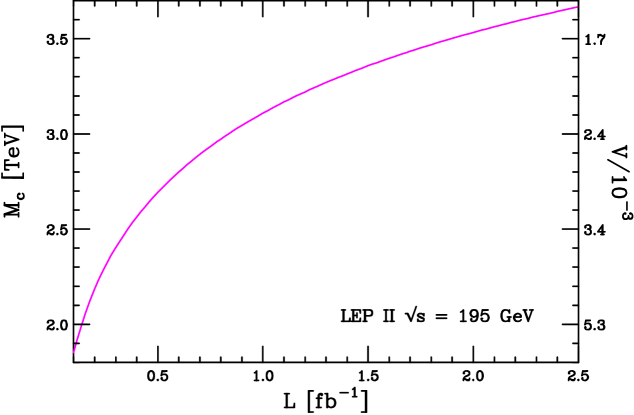
Figure 3: Search reach in $V$ at LEP2 running at $\sqrt{s}=195\hbox{\rm\,GeV}$ as a function of integrated luminosity. For the 5DSM the value of $V$ can be related to $M_{c}$, which is shown on the left vertical axis.

The same analysis can be applied at the NLC. However, here we are able to add the top quark to the list of final states. Furthermore, we can include polarization asymmetries at the NLC, and we can utilize observables associated with $\tau$ lepton polarization. At the NLC we assume that $b$, $t$ and $c$ quark identification efficiencies are $60\%$ and the efficiency for measuring tau polarization is 50% [85, 86].

The sensitivity to $V$ at the NLC is substantial. In Fig. 4 we plot the search reach for $V$ versus integrated luminosity for $\sqrt{s}=500\hbox{\rm\,GeV}$, $1000\hbox{\rm\,GeV}$ and $1500\hbox{\rm\,GeV}$ $e^{+}e^{-}$ colliders. With more than $500\hbox{\rm\, fb}^{-1}$ the reach is $V>12.5\times 10^{-5}$, $V>4.0\times 10^{-5}$, and $V>2.2\times 10^{-5}$ for the three ascending center-of-mass energies. In 5DSM, we can translate these reaches in $V$ into reaches of $M_{c}$ and find $13\hbox{\rm\,TeV}$, $23\hbox{\rm\,TeV}$ and $31\hbox{\rm\,TeV}$ respectively. These are significantly greater than for a typical GUT-inspired $Z^{\prime}$ [86] due to 1) the larger couplings (i.e., $\sqrt{2}$ enhancement), 2) the tower contribution, and 3) both $Z^{(n)}$ and $\gamma^{(n)}$ contribute.

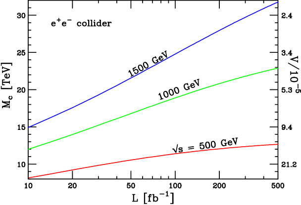
Figure 4: Search reach in $V$ at NLC running at $\sqrt{s}=500\hbox{\rm\,GeV}$, $1000\hbox{\rm\,GeV}$ and $1500\hbox{\rm\,GeV}$ as a function of integrated luminosity. For the 5DSM the value of $V$ can be related to $M_{c}$, which is shown on the left vertical axis.

4.2 Direct searches at hadron colliders

One can also look for direct production of the KK states at hadron colliders. We do not consider the capabilities of indirect, off-shell contributions of the KK excitations to hadron collider observables, since $Z^{\prime}$ studies indicate that the resonant production searches are more probing. The neutral current mode of producing final state lepton pairs in $Z^{(n)}/\gamma^{(n)}$ mediated Drell-Yan processes is the most useful mode to search for evidence of extra dimensions at the Tevatron and LHC.

The scattering processes $f\bar{f}\rightarrow l^{+}l^{-}$ through intermediate KK excitations $Z^{(n)}$ and $\gamma^{(n)}$ leads to peaks in the invariant mass spectrum at high-energies. The couplings of $Z^{(n)}$ and $\gamma^{(n)}$ to fermions is the same as their corresponding zero-mode couplings, except for an overall enhancement of $\sqrt{2}$. In our analysis we estimate the sensitivity to $M_{c}$ from only the first excited state. Incorporating other excited states into the search would yield a slightly higher sensitivity than what we present here.

The search strategy is based on leptonic final states in the narrow width approximation. For $Z^{(1)}$ first excited state with high mass, the search is for a narrow high-energy dilepton invariant mass excess. For $W^{(1)}$ at high mass, the search is for a high-energy lepton plus large missing energy. For a given luminosity the cuts are chosen such that no Standard Model background events are expected, and a signal is declared if there are more than 10 events presents given the same cuts. The strategy is summarized in ref. [86].

We can now present search capabilities for 1 extra dimension, the 5DSM, at the Tevatron and LHC. At the Tevatron with $\sqrt{s}=2\hbox{\rm\,TeV}$ and integrated luminosity of $2\hbox{\rm\, fb}^{-1}$ ($20\hbox{\rm\, fb}^{-1}$) we find that $M_{c}$ up to $1.20\hbox{\rm\,TeV}$ ($1.36\hbox{\rm\,TeV}$) can be probed in the combined neutral channels mediated by $\gamma^{(1)}$ and $Z^{(1)}$. At the LHC, in this same channel with $\sqrt{s}=14\hbox{\rm\,TeV}$ and $100\hbox{\rm\, fb}^{-1}$ integrated luminosity, we find a reach of up to $5.9\hbox{\rm\,TeV}$. Searches for the $W^{(1)}$ mode at the Tevatron allow discovery at $1.11\hbox{\rm\,TeV}$ and $1.34\hbox{\rm\,TeV}$ with $2\hbox{\rm\, fb}^{-1}$ and $20\hbox{\rm\, fb}^{-1}$ respectively. The $W^{(1)}$ can be discovered at the LHC with $100\hbox{\rm\, fb}^{-1}$ if its mass is less than $6.35\hbox{\rm\,TeV}$.

One could also look for enhancements in the dijet production at high invariant mass from KK excitations of the gluons. The procedure we employ here is similar to that used to constrain resonant production of squarks in theories with light gluinos [87]. We have extrapolated the CDF and D0 data to higher energies and luminosity, and find a reach capability of $M_{c}\lower 3.01385pt\hbox{$\;\stackrel{{\scriptstyle\textstyle<}}{{\sim}}\;$}700\hbox{\rm\,GeV}$, which is somewhat lower than the reach capability from $Z^{(1)}/\gamma^{(1)}$ and $W^{(1)}$ induced processes. At the LHC we estimate the reach of the first gluon excited level to be below $5\hbox{\rm\,TeV}$, although the precise number depends sensitively on the dijet energy resolution.

The search reach increases with more extra dimensions because there are more copies of the first KK excitation gauge bosons. For example, with one extra dimension presented above, there is only one copy of $Z^{(1)}$, $\gamma^{(1)}$ and $W^{(1)}$. With $d$ extra dimensions there are $d$ copies of these bosons, making a higher production rate of final state leptons for the same $M_{c}$. Also, with only one extra dimension the next KK excitation level is at $2M_{c}$ where only one copy of the gauge bosons reside, whereas with more than one extra dimension the next KK level is lower, $\sqrt{2}M_{c}$, where there may be many copies of the SM gauge bosons. Therefore, as the number of extra dimensions increases, it appears to become more important to consider the higher KK levels to get an accurate estimate of the maximum search reach. However, as discussed in section 2.3, the naive effective field theory description of KK excitations cannot be correct, especially for more than one extra dimension, and the couplings of the higher KK states must necessarily be suppressed in a model dependent way. For this reason, we have focussed only on the first excited state.

5 Conclusions

In conclusion, the Standard Model originating from more than four extra dimensions is just as good of a description of nature as the 4d Standard Model. The difference is in the allowed physical parameters that have not yet been detected. For example, in the ordinary 4DSM, the Higgs boson mass must be less than about $260\hbox{\rm\,GeV}$ in order for the precision electroweak data to match the data well. This is not the case in the 5DSM, where much larger masses (up to $500\hbox{\rm\,GeV}$) for the Higgs boson are allowed as long as the Higgs boson is confined to the wall and KK excitations of the gauge bosons are rather light.

Table 2 contains a summary of many of the results presented in the text. All results have been translated into bounds or sensitivity on the compactification scale in the 5DSM, where one can see that current and future colliders will be able to probe well into the TeV region. This is especially relevant for the solution to the hierarchy problem, which we view as the strongest motivations for this scenario. If low-scale compactification theories do have some relevance for electroweak symmetry breaking and the hierarchy problem, it is then at the TeV scale that we expect evidence for them to show up. This is directly analogous to expectations for finding supersymmetry, since low-scale supersymmetry also solves the hierarchy problem. The scale of $M_{c}$ can then be thought of in the same way as the scale of superpartner masses and the ratio $m_{W}^{2}/M_{c}^{2}$ is one measure of how fine-tuned the electroweak potential is. It is for these reasons that we are optimistic that low-scale, sub-Planckian compactifications are more likely at lower scales near $m_{W}$ than at higher, inaccessible scales.

Experiment	$M_{c}$ reach
PEW with Higgs in bulk	$3.8\hbox{\rm\,TeV}$
PEW with Higgs on wall	$3.3\hbox{\rm\,TeV}$
LEPII with $\sqrt{s}=195\hbox{\rm\,GeV}$ and $L=1\hbox{\rm\, fb}^{-1}$	$3.1\hbox{\rm\,TeV}$
Tevatron with $\sqrt{s}=2\hbox{\rm\,TeV}$ and $L=2\hbox{\rm\, fb}^{-1}$	$1.1\hbox{\rm\,TeV}$
Tevatron with $\sqrt{s}=2\hbox{\rm\,TeV}$ and $L=20\hbox{\rm\, fb}^{-1}$	$1.3\hbox{\rm\,TeV}$
LHC with $\sqrt{s}=14\hbox{\rm\,TeV}$ and $L=100\hbox{\rm\, fb}^{-1}$	$6.3\hbox{\rm\,TeV}$
NLC with $\sqrt{s}=500\hbox{\rm\,GeV}$ and $L=500\hbox{\rm\, fb}^{-1}$	$13\hbox{\rm\,TeV}$
NLC with $\sqrt{s}=1000\hbox{\rm\,GeV}$ and $L=500\hbox{\rm\, fb}^{-1}$	$23\hbox{\rm\,TeV}$
NLC with $\sqrt{s}=1500\hbox{\rm\,GeV}$ and $L=500\hbox{\rm\, fb}^{-1}$	$31\hbox{\rm\,TeV}$

Table 2: Summary of search reaches of the compactification scale in the 5DSM with different experiments. PEW stands for precision electroweak data accumulated at LEP, SLD, NuTeV, etc. The hadron collider numbers are for direct production sensitivity of the first KK excited states of the gauge bosons, and the high-energy $e^{+}e^{-}$ collider numbers are for inferred limits from deviations in fermion final state observables below on-shell threshold.

Acknowledgements: We thank F. del Aguila, T. Gherghetta, G. Giudice, J. Hewett, M. Masip and A. Pomarol for helpful conversations. TGR thanks the CERN Theory Division, where part of this was done, for its hospitality.

References

- [1]
- [2] T. Appelquist, A. Chodos, and P.G.O. Freund (eds.), Modern Kaluza-Klein Theories, Addison-Wesley Publishing Company: Menlo Park, California, USA (1987).
- [3] L. O’Raifeartaigh and N. Straumann, “Early history of gauge theories and Kaluza-Klein theories,” hep-ph/9810524.
- [4] M. Green, J.H. Schwarz, and E. Witten, Superstring Theory, two volumes, Cambridge University Press: Cambridge, UK (1987).
- [5] J. Polchinski, Introduction to String Theory, two volumes, Cambridge University Press: Cambridge, UK (1998).
- [6] N. Arkani-Hamed, S. Dimopoulos, and G. Dvali, “The hierarchy and new dimensions at a millimeter,” Phys. Lett. B 429, 263 (1998) [hep-ph/9803315].
- [7] N. Arkani-Hamed, S. Dimopoulos, and G. Dvali, “Phenomenology, astrophysics and cosmology of theories with submillimeter dimensions and TeV scale quantum gravity,” Phys. Rev. D 59, 086004 (1999) [hep-ph/9807344].
- [8] I. Antoniadis, N. Arkani-Hamed, S. Dimopoulos, and G. Dvali, “New dimensions at a millimeter to a fermi and superstrings at a TeV,” Phys. Lett. B 436, 257 (1998) [hep-ph/9804398].
- [9] R. Sundrum, “Towards an effective particle-string resolution of the cosmological constant problem,” hep-ph/9708329.
- [10] N. Arkani-Hamed, S. Dimopoulos, and J. March-Russell, “Stabilization of submillimeter dimensions: the new guise of the hierarchy problem,” hep-th/9809124.
- [11] E. Witten, “Strong coupling expansion of Calabi-Yau compactification,” Nucl. Phys. B 471, 135 (1996) [hep-th/9602070].
- [12] P. Horava and E. Witten, “Heterotic and type I string dynamics from eleven dimensions,” Nucl. Phys. B 460, 506 (1996) [hep-th/9510209].
- [13] P. Horava and E. Witten, “Eleven-dimensional supergravity on a manifold with boundary,” Nucl. Phys. B 475, 94 (1996) [hep-th/9603142].
- [14] C. Kounnas and M. Porrati, “Spontaneous supersymmetry breaking in string theory,” Nucl. Phys. B 310, 355 (1988).
- [15] S. Ferrara, C. Kounnas, M. Porrati, and F. Zwirner, “Superstrings with spontaneously broken supersymmetry and their effective theories,” Nucl. Phys. B 318, 75 (1989).
- [16] I. Antoniadis, “A possible new dimension at a few TeV,” Phys. Lett. B 246, 377 (1990).
- [17] J.D. Lykken, “Weak scale superstrings,” Phys. Rev. D 54, 3693 (1996) [hep-th/9603133].
- [18] G. Shiu and S.H.H. Tye, “TeV scale superstring and extra dimensions,” Phys. Rev. D 58, 106007 (1998) [hep-th/9805157].
- [19] Z. Kakushadze and S.H.H. Tye, “Brane world,” hep-th/9809147.
- [20] K.R. Dienes, E. Dudas, and T. Gherghetta, “Extra space-time dimensions and unification,” Phys. Lett. B 436, 55 (1998) [hep-ph/9803466].
- [21] K.R. Dienes, E. Dudas, and T. Gherghetta, “Grand unification mass scales through extra dimensions,” Nucl. Phys. B 537, 47 (1999) [hep-ph/9806292].
- [22] D. Ghilencea and G.G. Ross, “Unification and extra space-time dimensions,” Phys. Lett. B 442, 165 (1998) [hep-ph/9809217].
- [23] Z. Kakushadze, “Novel extension of MSSM and TeV scale coupling unification,” hep-th/9811193.
- [24] C.D. Carone, “Gauge unification in nonminimal models within extra dimensions,” hep-ph/9902407.
- [25] A. Delgado and M. Quiros, “Strong coupling unification and extra dimensions,” hep-ph/9903400.
- [26] P.H. Frampton and A. Rasin, “Unification with enlarged Kaluza-Klein dimensions,” hep-ph/9903479.
- [27] A. Perez-Lorenzana and R.N. Mohapatra, “Effect of extra dimensions on gauge coupling unification,” hep-ph/9904504.
- [28] Z. Kakushadze and T.R. Taylor, “Higher loop effects on unification via Kaluza-Klein thresholds,” hep-th/9905137.
- [29] I. Antoniadis and K. Benakli, “Limits on extra dimensions in orbifold compactifications of superstrings,” Phys. Lett. B 326, 69 (1994) [hep-th/9310151].
- [30] I. Antoniadis, K. Benakli, and M. Quiros, “Production of Kaluza-Klein states at future colliders,” Phys. Lett. B 331, 313 (1994) [hep-ph/9403290].
- [31] P. Nath and M. Yamaguchi, “Effects of extra space-time dimensions on the Fermi constant,” hep-ph/9902323.
- [32] M. Masip and A. Pomarol, “Effects of SM Kaluza-Klein excitations on electroweak observables,” hep-ph/9902467.
- [33] P. Nath and M. Yamaguchi, “Effects of Kaluza-Klein excitations on ,” hep-ph/9903298.
- [34] W.J. Marciano, “Fermi constants and new physics,” hep-ph/9903451.
- [35] I. Antoniadis, K. Benakli, and M. Quirós, “Direct collider signatures of large extra dimensions,” hep-ph/9905311.
- [36] P. Nath, Y. Yamada, and M. Yamaguchi, “Probing the nature of compactification with Kaluza-Klein excitations at the Large Hadron Collider,” hep-ph/9905415.
- [37] G.F. Giudice, R. Rattazzi, and J.D. Wells, “Quantum gravity and extra dimensions at high-energy colliders,” Nucl. Phys. B 544, 3 (1999) [hep-ph/9811291].
- [38] E.A. Mirabelli, M. Perelstein, and M.E. Peskin, “Collider signatures of new large space dimensions,” Phys. Rev. Lett. 82, 2236 (1999) [hep-ph/9811337].
- [39] J.L. Hewett, “Indirect collider signals for extra dimensions,” hep-ph/9811356.
- [40] T. Han, J.D. Lykken, and R.-J. Zhang, “On Kaluza-Klein states from large extra dimensions,” Phys. Rev. D 59, 105006 (1999) [hep-ph/9811350].
- [41] P. Mathews, S. Raychaudhuri, and K. Sridhar, “Getting to the top with extra dimensions,” Phys. Lett. B 450, 343 (1999) [hep-ph/9811501].
- [42] T.G. Rizzo, “More and more indirect signals for extra dimensions at more and more colliders,” Phys. Rev. D 59, 115010 (1999) [hep-ph/9901209].
- [43] T.G. Rizzo, “Top quark production at the Tevatron: probing anomalous chromomagnetic moments and theories of low scale gravity,” Talk given at Physics at RUN II: Workshop on Top Physics, Batavia, IL, 16-18 Oct 1998, hep-ph/9902273.
- [44] M.L. Graesser, “Extra dimensions and the muon anomalous magnetic moment,” hep-ph/9902310.
- [45] T. Banks, M. Dine, and A. Nelson, “Constraints on theories with large extra dimensions,” hep-th/9903019.
- [46] S.P. Martin and J.D. Wells, “Motivation and detectability of an invisibly decaying Higgs boson at the Fermilab Tevatron,” hep-ph/9903259.
- [47] T.G. Rizzo, “Using scalars to probe theories of low scale quantum gravity,” hep-ph/9903475.
- [48] D. Atwood, S. Bar-Shalom, and A. Soni, “Graviton production by two photon processes in Kaluza-Klein theories with large extra dimensions,” hep-ph/9903538.
- [49] P. Mathews, S. Raychaudhuri, and K. Sridhar, “Testing TeV scale quantum gravity using dijet production at the Tevatron,” hep-ph/9904232.
- [50] K. Cheung, “Diphoton signals for low scale gravity in extra dimensions,” hep-ph/9904266.
- [51] K.Y. Lee, H.S. Song and J.H. Song, “Polarization effects on the process with large extra dimensions,” hep-ph/9904355 .
- [52] T.G. Rizzo, “Tests of low scale gravity via gauge boson pair production in gamma gamma collisions,” hep-ph/9904380.
- [53] H. Davoudiasl, “ as a test of weak scale quantum gravity at the NLC,” hep-ph/9904425.
- [54] C. Balazs, H.-J. He, W.W. Repko, C.-P. Yuan, and D.A. Dicus, “Collider tests of compact space dimensions using weak gauge bosons,” hep-ph/9904220.
- [55] K. Cheung, “Global lepton quark neutral current constraint on low scale gravity model,” hep-ph/9904510.
- [56] K.Y. Lee, H.S. Song, J.-H. Song, and C. Yu, “Large extra dimension effects on the spin configuration of the top quark pair at colliders,” hep-ph/9905227 .
- [57] X.G. He, “Extra dimensions and Higgs pair production at photon colliders,” hep-ph/9905295.
- [58] P. Mathews, P. Poulose, and K. Sridhar, “Probing large extra dimensions using top production in photon-photon collisions,” hep-ph/9905395.
- [59] T. Han, D. Rainwater, and D. Zeppenfeld, “Drell-Yan plus missing energy as a signal for extra dimensions,” hep-ph/9905423.
- [60] K. Benakli and S. Davidson, “Baryogenesis in models with a low quantum gravity scale,” hep-ph/9810280.
- [61] S. Cullen and M. Perelstein, “SN1987A constraints on large compact dimensions,” hep-ph/9903422.
- [62] L.J. Hall and D. Smith, “Cosmological constraints on theories with large extra dimensions,” hep-ph/9904267.
- [63] V. Barger, T. Han, C. Kao, and R.-J. Zhang, “Astrophysical constraints on large extra dimensions,” hep-ph/9905474.
- [64] L.J Hall and C. Kolda, “Electroweak symmetry breaking and large extra dimensions,” hep-ph/9904236.
- [65] A. Pomarol and M. Quiros, “The Standard Model from extra dimensions,” Phys. Lett. B 438, 255 (1998) [hep-ph/9806263].
- [66] I. Antoniadis, S. Dimopoulos, A. Pomarol, and M. Quiros, “Soft masses in theories with supersymmetry breaking by TeV compactification,” Nucl. Phys. B 544, 503 (1999) [hep-ph/9810410].
- [67] A. Delgado, A. Pomarol, and M. Quiros, “Supersymmetry and electroweak breaking from extra dimensions at the TeV scale,” hep-ph/9812489.
- [68] Z. Kakushadze, “TeV scale supersymmetric standard model and brane world,” hep-th/9812163.
- [69] Z. Kakushadze, “Flavor ’conservation’ and hierarchy in TeV scale supersymmetric standard model,” hep-th/9902080.
- [70] I. Antoniadis, C. Muñoz, and M. Quirós, “Dynamical supersymmetry breaking with a large internal dimension,” Nucl. Phys. B 397, 515 (1993) [hep-ph/9211309].
- [71] N. Arkani-Hamed and M. Schmaltz, “Hierarchies without symmetries from extra dimensions,” hep-ph/9903417.
- [72] G. Shiu, R. Shrock and S.H. Henry Tye, “Collider signatures from the brane world,” hep-ph/9904262.
- [73] C.P. Bachas, “Unification with low string scale,” JHEP 11, 023 (1998) [hep-ph/9807415].
- [74] I. Antoniadis and C. Bachas, “Branes and the gauge hierarchy,” Phys. Lett. B 450, 83 (1999) [hep-th/9812093].
- [75] D. Bardin, “ZFITTER: An analytical program for fermion pair production in annihilation,” hep-ph/9412201.
- [76] T. van Ritbergen and R.G. Stuart, “On the precise determination of the Fermi coupling constant from the muon lifetime,” hep-ph/9904240.
- [77] L. DiLella, “Experiment summary,” Talk given at the 34th Rencontres de Moriond: Electroweak interactions and unified theories, 13-20 March 1999 Les Arcs, France [http://moriond.in2p3.fr/EW/transparencies/99/07_Saturday/Dilella/index.html].
- [78] S.C. Bennett and C.E. Wieman, “Measurement of the transition polarizability in atomic cesium and an improved test of the Standard Model,” Phys. Rev. Lett. 82, 2484 (1999) [hep-ex/9903022].
- [79] NuTeV Collaboration (K.S. McFarland et al.), “Measurement of from neutrino nucleon scattering at NuTeV,” hep-ex/9806013.
- [80] LEP Electroweak Working Group (D. Abbaneo et al.), “A Combination of Preliminary Electroweak Measurements and Constraints on the Standard Model,” CERN-EP/99-15 (8 February 1999).
- [81] M. Davier and A. Hocker, “Improved determination of and the anomalous magnetic moment of the muon,” Phys. Lett. B 419, 419 (1998) [hep-ph/9711308].
- [82] G.J. Feldman and R.D. Cousins, “Unified approach to the classical statistical analysis of small signals,” Phys. Rev. D 57, 3873 (1998).
- [83] L3 Collaboration, “Standard model Higgs searches at ,” L3 Note 2382 (March 1999); DELPHI Collaboration, “Search for neutral Higgs bosons in the Standard Model and the MSSM at 189 GeV,” DELPHI 99-8 (March 1999); ALEPH Collaboration, “Search for the neutral Higgs bosons of the Standard Model and the MSSM in collisions at ,” ALEPH 99-007 (March 1999); OPAL Collaboration, “Search for neutral Higgs bosons in collisions at ,” OPAL PN382 (March 1999).
- [84] R. Barbieri and A. Strumia, “What is the limit on the Higgs mass?,” hep-ph/9905281.
- [85] NLC ZDR Design Group and NLC Physics Working Group (S. Kuhlman et al.), “Physics and technology of the Next Linear Collider: a report submitted to Snowmass 96,” hep-ex/9605011.
- [86] T.G. Rizzo, “Extended gauge sectors at future colliders: report of the new gauge boson subgroup,” Proceedings of the 1996 DPF/DPB Summer Study on New Directions for High Energy Physics – Snowmass 96, Snowmass, Colorado, 25 June - 12 July 1996 [hep-ph/9612440].
- [87] J.L. Hewett, T.G. Rizzo, and M.A. Doncheski, “Constraints on light gluinos from Tevatron dijet data,” Phys. Rev. D 56, 5703 (1997) [hep-ph/9612377].